Coordination on List Prices

and Collusion in Negotiated Prices∗

Joseph E. Harrington, Jr.†and Lixin Ye‡

1 April 2017

Abstract

A collusive practice in some intermediate goods markets is for sellers to co-

ordinate on list prices but not final prices. We put forth a theory to explain how

coordination on list prices can raise transaction prices even when all customers

pay negotiated prices. Market conditions are identified that are conducive to

firms profitably engaging in this form of collusive practice.

∗The comments of participants at the 2016 Hal White Antitrust Conference (Washington, D.C.),

2016 UBC Industrial Organization Conference (Kelowna, British Columbia), and a seminar at the

Norwegian School of Economics are gratefully acknowledged, as is the extremely able research assis-

tance of Ben Rosa and Xingtan (Ken) Zhang. The first author recognizes the financial support of

the National Science Foundation (SES-1148129).†Department of Business Economics & Public Policy, The Wharton School, University of Penn-

sylvania, Philadelphia, PA 19104, harrij@wharton.upenn.edu‡Department of Economics, Ohio State University, Columbus, OH 43210, ye.45@osu.edu

1

1 Introduction

Collusion entails firms coordinating on the prices that they charge customers. In

the context of retail markets, firms agree to supracompetitive posted prices and then

monitor each other to ensure that those are the prices charged in stores (or online).

With intermediate goods markets, it is more complicated because firms set list prices

and routinely offer discounts to buyers. While they may agree on list prices, it is

really the coordination on final transaction prices that is essential, as noted for the

thread cartel:1

[A cartel member] explained that list prices have more of a political

importance than a competitive one. Only very small clients pay the prices

contained in the lists. As the offi cial price lists issued by each competitor

are based on large profit margins, customers regularly negotiate rebates,

but no clear or fixed amount of rebates is granted. ... Therefore, the list

prices are essentially "fictitious" prices ... while [rebates] were discussed

and agreed during the meetings.

Once having coordinated on list prices and discounts, the challenge is then moni-

toring for compliance. While list prices are public information, discounts are privately

negotiated between a buyer and seller which makes it diffi cult to determine whether

cartel members charged the agreed-upon final transaction prices. The solution pur-

sued by many cartels - including those in the markets for citric acid, lysine, and

vitamins - was to agree to an allocation of sales quotas along with final transaction

prices, and then monitor for compliance by comparing realized sales to those quotas.2

Contrary to the rather standard collusive practices just described, some interme-

diate goods cartels coordinated exclusively on list prices and left firms unconstrained1Commission of the European Communities, 14.09.2005, Case COMP/38337/E1/PO/Thread,

112, 159-60.2Harrington (2006), Connor (2008), and Marshall and Marx (2012) provide details on these and

other relevant cartels. For an analysis of this collusive practice and related ones, see Harrington and

Skrzypacz (2011), Chan and Zhang (2015), Spector (2015), Awaya and Krishna (2016), and Sugaya

and Wolitzky (2016).

2

in the discounts that they offered. Furthermore, there was no evidence of sales moni-

toring to ensure that firms did not gain market share through discounts and, in fact,

discounts were regularly given to customers. This pattern occurred in several private

litigation cases for which plaintiffs, defendants, and the court often came to different

conclusions regarding the effi cacy of firms coordinating on list prices.3

Reserve Supply v. Owens-Corning Fiberglas (1992) concerned possible collusion

in the market for insulation. Plaintiffs and defendants put forth conflicting claims

regarding the collusive role of list prices:4

Reserve points to Owens-Corning and CertainTeed’s practices of main-

taining price lists for products and ... asserts that these lists have no

independent value because no buyer in the industry pays list price for

insulation. Instead, it claims that the price lists are an easy means for

producers to communicate and monitor the price activity of rivals by

providing a common starting point for the application of percentage dis-

counts. ... Owens-Corning and CertainTeed counter by arguing that the

use of list prices to monitor pricing would not be possible because the

widespread use of discounts in the industry ensures that list prices do not

reflect the actual price that a purchaser pays.

The Seventh Circuit Court expressed skepticism with regards to the plaintiffs’claim:5

We agree that the industry practice of maintaining price lists and

announcing price increases in advance does not necessarily lead to an in-

ference of price fixing. ... [T]his pricing system would be, to put it mildly,

an awkward facilitator of price collusion because the industry practice of

providing discounts to individual customers ensured that list price did not

reflect the actual transaction price.

3 In addition to the cases mentioned below is Lum v. Bank of America 361 F.3d, 217, 231 (3d

Cir., 2004). For that case, also see the discussion in Holmes (2004).4Reserve Supply v. Owens-Corning Fiberglas 971 F. 2d 37 (7th Cir. 1992), para 61.5 Ibid, para. 62.

3

In a case involving the market for urethane, plaintiffs claimed:6

[T]hroughout the alleged conspiracy period, the alleged conspirators

announced identical price increases simultaneously or within a very short

time period. ... [P]urchasers could negotiate down from the increased

price. But the increase formed the baseline for negotiations. ... [T]he

announced increases caused prices to rise or prevented prices from falling

as fast as they otherwise would have.

The Tenth Circuit Court quoted the District Court in supporting this assessment:7

The court reasoned that the industry’s standardized pricing structure -

reflected in product price lists and parallel price-increase announcements -

“presumably established an artificially inflated baseline”for negotiations.

Consequently, any impact resulting from a price-fixing conspiracy would

have permeated all polyurethane transactions, causing market-wide im-

pact despite individualized negotiations.

A final example is a recent cement cartel in the United Kingdom.8 Annually,

cement suppliers sent letters to their customers announcing price increases. However,

prices were then individually negotiated with customers and the full price increase

was rarely implemented. The Competition and Markets Authority concluded that

the price announcement letters served to coordinate on list prices and this impacted

the subsequent negotiations:9

We understand, however, that the prices set out in price increase let-

ters are in practice used as a starting point for negotiations with customers

6Class Plaintiffs’Response Brief (February 14, 2014), In Re: Urethane Antitrust Litigation, No.

13-3215, 10th Cir.; pp. 8-9.7 In Re: Urethane Antitrust Litigation, No. 13-3215 (10th Cir. Sep. 29, 2014); p. 7.8“Aggregates: Report on the market study and proposed decision to make a market investigation

reference,”Offi ce of Fair Trading, OFT1358, August 2011.9 Ibid, p. 53.

4

and that firms generally fail to achieve the prices set out in the price let-

ters, in part because of the rebates offered to large customers. This failure

to achieve "list" prices suggests that prices are not simply fixed through

this mechanism [that is, price announcement letters].

Though the coordination in list prices did not involve express communication, it

is the same pattern as with the cases involving insulation and urethane: Sellers

coordinated on list prices but not transaction prices. In commenting on the UK

cement case, Justin Coombs, who is head of Compass Lexecon’s London offi ce, posed

the question: “How do price announcements help firms coordinate on prices if prices

are ultimately individually negotiated?”10 To our knowledge, there is no theory that

provides an answer to that question.

Our objective is to explore the possibility that firms could successfully collude

by coordinating only on list prices while leaving firms with complete discretion in

setting final transaction prices. The two questions addressed here are: 1) How can

coordination in list prices result in supracompetitive transaction prices?; and 2) Hav-

ing identified a mechanism whereby list prices impact negotiated prices, what market

conditions are conducive to firms profitably engaging in this form of collusive prac-

tice?

Section 2 describes the model, while a review of some related research is provided

in Section 3. There are two steps to developing the theoretical argument. First

is establishing an endogenous connection between announced list prices and final

transaction prices, which is conducted in Section 4. The second step is showing

that firms can jointly raise profits by coordinating their list prices. That is done in

Sections 5-7. Section 8 illustrates how this theoretical insight can provide guidance

in antitrust cases. Unless otherwise noted, proofs are in the appendix.

10“Exchange of Information: Current Issues,”30 April 2014, Allen & Overy, Brussels.

5

2 Model

Consider a market with two sellers offering identical products. A seller may be one

of two types, L or H, and type L occurs with probability q. Sellers’types are inde-

pendent. A type t seller’s unit cost is assumed to be a random draw from the cdf

Ft : [ct, ct] → [0, 1], t ∈ {L,H} . Ft is continuously differentiable with positive den-

sity everywhere on (ct, ct). The inverse hazard rate function, ht(c) ≡ Ft(c)/F′t(c), is

assumed to be non-decreasing, h′t(c) ≥ 0, which holds for most of the common distri-

butions such as uniform, normal, exponential, logistic, chi-squared, and Laplace. The

two cost distributions are ranked in terms of their inverse hazard rates: hL(c) > hH(c)

for all c ∈ (ct, ct]. Note that the latter condition implies FH first-order stochastically

dominates FL and, consequently, we will refer to a type L seller as a low-cost type

and a type H seller as a high-cost type.

Each buyer is interested in buying 0 or 1 unit and v denotes a buyer’s valuation.

There is a continuum of buyers and their valuations are represented by the cdf G :

[v, v] → [0, 1]. G is continuously differentiable with positive density everywhere on

(v, v). A buyer may choose to solicit offers from either 1 or 2 sellers. What exactly

it means to “solicit” an offer is described below. A fraction b ∈ [0, 1] of sellers are

assumed to solicit an offer from a single seller and a fraction 1 − b from two sellers.

Whether a buyer approaches 1 or 2 sellers is assumed to be independent of a buyer’s

valuation.11

The modelling of the interaction between buyers and sellers is intended to capture

many intermediate goods markets for which buyers are industrial customers. Sellers

first choose list (or posted) prices. After observing those list prices, each buyer

approaches either 1 or 2 sellers to negotiate. A buyer who approaches two sellers is

presumed to engage in an iterative bargaining process whereby she uses an offer from

11Though it would be preferable to endogenize the number of sellers that are solicited by a buyer, it

is assumed to be exogenous for reasons of tractability. This specification could be trivially rationalized

by assuming buyers incur a cost to negotiating with each seller, they vary in this cost, and the cost

is independent of a buyer’s valuation. Some buyers have very low cost and thus negotiate with both

sellers, while other buyers have a high enough cost that it is optimal to only negotiate with one seller.

6

one seller to obtain a better offer from the other seller. Rather than explicitly model

that process, we will use the second-price auction with a reserve price as a metaphor

for it. More specifically, a buyer “invites”w sellers to the auction, where w ∈ {1, 2} .

The buyer sets a reserve price and the w sellers submit bids which, in equilibrium,

will equal their cost. We have buyers choose a reserve price so they are not passive,

which better mimics negotiation.12 A transaction occurs if the lowest bid is below

the buyer’s reserve price. In the case of having chosen just one seller, the mechanism

is equivalent to the buyer making a take it or leave it offer. List prices are presumed

to be chosen less frequently than negotiated prices and this has the implication that

a seller knows its cost type when it chooses its list price but does not know its actual

cost until the time of negotiation. In practice, this uncertainty about future cost may

be due to volatility in input prices or not knowing the opportunity cost of supply

because future inventories or capacity constraints are uncertain.

As our focus is on markets for which very few, if any, consumers fail to negotiate

the price that they pay, it will make for a more parsimonious analysis if we presume

that no transactions take place at list price by supposing a list price is a cheap talk

message and not actually a price at which buyers can transact. As in the thread

cartel mentioned in the introduction, list prices are then “fictitious” but, as we’ll

show, can still be informative and impactful.

The extensive form is as follows:

• Stage 1: Sellers draw types from {L,H} (which is private information to each

seller) and choose a list price (which is a cheap talk message) from {l, h} .

• Stage 2: Buyers learn their valuations, observe sellers’list prices, and choose w

sellers where w ∈ {1, 2} .

• Stage 3: Each seller realizes its cost. If a seller is type t then its cost is a draw

from [ct, ct] according to Ft.

12As sellers optimally submit bids equal to their costs, it does not matter if the reserve price is

hidden or not.

7

• Stage 4: For each buyer, the w selected sellers participate in a second-price

auction with a hidden reserve price. Each seller submits a bid equal to its cost.

Transactions and transaction prices are determined as follows:

— If there are two sellers in the auction and

∗ both bids are below the reserve price then the buyer buys from the

seller with the lowest bid at a price equal to the second lowest bid.

∗ one bid is below the reserve price and the other bid is above the reserve

price then the buyer buys from the seller with the lowest bid at a price

equal to the reserve price.

∗ both bids are above the reserve price then there is no transaction.

— If there is one seller in the auction and

∗ the bid is below the reserve price then the buyer buys from the seller

at the reserve price.

∗ the bid is above the reserve price then there is no transaction.

A strategy for a seller is a pair of functions: a list price function and a bid

function. The list price function maps from {L,H} to {l, h} and thus has a seller

select a list price based on its cost type. In the event a seller is selected by a buyer,

a bid function assigns a bid depending on the seller’s cost type, the seller’s cost, the

other seller’s list price, and whether the buyer selected one or two sellers. The weakly

dominant bidding strategy for a seller is to bid its cost. From hereon, we will think of

a strategy for a seller as a list price function and a bid function that has its bid equal

to its cost. In that case, there are four strategies, associated with the four ways in

which to map {L,H} to {l, h} . For a buyer who is restricted to choosing one seller, a

strategy selects a seller and a reserve price conditional on the observed list prices and

the buyer’s valuation. If the buyer chooses two sellers, a strategy selects a reserve

price conditional on the observed list prices and the buyer’s valuation. The solution

concept is perfect Bayes-Nash equilibrium.

8

3 Literature Review

There is a small body of work that examines firms setting list prices and offering

discounts. Chen and Rosenthal (1996), García Díaz, Hernán González, and Kujal

(2009), Raskovich (2007), and Lester, Visschers, and Wolthoff (2015) have sellers

post a list price which is subsequently followed by either discounts or negotiation.

Those papers do not consider collusion and the driving forces to their analyses are

distinct from that which operates in our model. Gill and Thanassoulis (2016) is the

only paper to consider collusion but it assumes firms coordinate on both list and

discounted prices. There is no previous research for which firms collude on list prices

and compete in discounts or on negotiated prices.

This paper also relates to research on directed search in a market setting. Directed

search is present in our model in that list prices may direct buyers to negotiate

with certain sellers. One strand of literature concerns indicative bidding which is a

two-stage auction process commonly used in the sales of business assets with very

high values. In the first stage, potentially interested buyers submit non-binding

bids. These bids are meant to be indicative of bidders’ interest in the item for

sale. The highest of these non-binding bids, in conjunction with decisions regarding

bidders’qualifications, are then used to establish a short list of final (second-stage)

bidders who participate in a first-price sealed-bid auction. Ye (2007) provides the

first study of indicative bidding and allows for costly information acquisition. The

analysis suggests that the current design of indicative bidding cannot reliably select

the most qualified bidders for the final sale, as there does not exist a symmetric,

strictly increasing equilibrium bid function in the indicative bidding stage; hence,

bidders do not truthfully reveal their types. By restricting indicative bids to a finite

domain, Quint and Hendricks (2015) explicitly model indicative bidding as cheap talk

with commitment, and show that a symmetric equilibrium exists in weakly-monotone

strategies. But again, the highest-value bidders are not always selected, as bidder

types “pool”over a finite number of bids. Our paper differs from Ye (2007) and Quint

and Hendricks (2015) mainly in that no entry cost is assumed for bidders, and that

9

the reserve price in the final selling mechanism depends on the list prices (indicative

bids). As such, a separating equilibrium in the cheap-talk stage becomes possible in

our setting.

Menzio (2007) considers cheap talk in a search model of a competitive labor

market. Employers have private information about the quality of their vacancies

and can costlessly communicate with unemployed workers before they engage in an

alternating offer bargaining game to determine the wage. It is shown that unless the

labor market is either too tight or too slack, there exists an equilibrium in which

noncontractual announcements (cheap talk) about compensation is correlated with

actual wages and, therefore, it serves to direct the search of workers. As we explain

later, our theory encompasses the driving forces in Menzio (2007) though in the

context of an imperfectly competitive product market setting.

Finally, Kim and Kircher (2015) introduce cheap talk into an otherwise canonical

competing auctions setting. In their model, auctioneers with private reservation

values compete for bidders by announcing cheap-talk messages. They show that the

choice of the trading mechanism is critical. When the first-price auction is used,

there always exists an equilibrium in which each auctioneer truthfully reveals her

type. When the second-price auction is used, however, no informative equilibrium

exists.

4 Strategies Under Competition and Collusion

A critical element to the ensuing theory is the descriptively realistic assumption

that buyers are uncertain whether sellers are competing or colluding.13 Let κ (for

the German "kartell") denote the probability that buyers assign to firms colluding.

Consistent with the low level of documented cartels, it is presumed that κ > 0 but

13That other agents - whether buyers, the competition authority, or potential entrants - are un-

certain about whether market outcomes are the product of competition or collusion is assumed, for

example, in Harrington (1984), Besanko, and Spulber (1989, 1990), LaCasse (1995), Schinkel and

Tuinstra (2006), and Souam (2001).

10

small. It will become clear where we use the presumption that κ is small.14 Buyers

are assumed to live for only one period and do not observe the history.15

Suppose firms are competing which means that their strategies must form a perfect

Bayes-Nash equilibrium for the one-shot game. As this is a cheap talk game, there

are always pooling equilibria which, in our setting, means uninformative list prices.16

We will focus on equilibria in which a seller’s list price is informative of its cost type.

Hence, consider sellers using the separating strategy that has a low-cost (high-cost)

type post a low (high) list price:

φ(t) =

l if t = L

h if t = H(1)

Alternatively, firms are colluding which will mean that they use a pooling strategy

whereby a seller announces a high list price regardless of its cost type:

ψ(t) =

h if t = H

h if t = H(2)

The value of coordinating their list prices in this manner is explained below.

Given a prior probability κ that firms are colluding and using (2) and probability

1 − κ that firms are competing and using (1), a buyer’s beliefs as to sellers’ types14Obviously, evidence is based on discovered cartels and, based on that evidence, the fraction of

markets with documented cartels is very small. Of course, there could be many undiscovered cartels

so that the frequency of cartels is, in fact, not small. What is important for the analysis is that

buyers believe cartels are infrequent which seems highly plausible for most markets.15Though this assumption is inconsistent with them being industrial buyers, it allows us to avoid

a diffi cult dynamic problem. If buyers were long-lived and observed the past then they would update

their beliefs over time regarding the hypothesis that there is collusion. While characterizing buyers’

beliefs over time is not a problem in and of itself, colluding sellers would take into account how their

current actions (both with regards to list prices and bids) impacts buyers’ beliefs and the future

value of collusion. Thus, it now becomes a dynamic game between buyers and sellers. That is clearly

a setting worth examining but is one we leave to future research.16With those equilibria, a seller’s strategy is to choose h with some probability s ∈ [0, 1] if type

L or H, and then bid its realized cost if selected by a buyer. A buyer’s beliefs on a seller’s type are

the prior beliefs: If l or h is observed then a seller is type L with probability q. A buyer chooses an

optimal reserve price based on those prior beliefs.

11

given their list prices can be derived. When buyers observe either or both sellers

posting a low list price, they infer that firms are competing. Letting mi denote the

message and ti denote the type of firm i, respectively, posterior beliefs (conditional

on list prices) are:

• If (m1,m2) = (l, l) then firms are competing and Pr(ti = L |(m1,m2) = (l, l)) =

1, i = 1, 2.

• If (m1,m2) = (l, h) then firms are competing and Pr(t1 = L |(m1,m2) = (l, h)) =

1,Pr(t2 = H |(m1,m2) = (l, h)) = 1.

• If (m1,m2) = (h, l) then firms are competing and Pr(t1 = H |(m1,m2) = (h, l)) =

1,Pr(t2 = L |(m1,m2) = (h, l)) = 1.

However, when buyers observe both sellers posting high list prices, they do not know

whether sellers are competing (and are high-cost types) or are colluding. Bayesian

updating implies:

Pr(ti = L |(m1,m2) = (h, h)) =κq

κ+ (1− κ)(1− q) (3)

Pr(ti = H |(m1,m2) = (h, h)) =1− q

κ+ (1− κ)(1− q) , i = 1, 2.

With these beliefs on sellers’types, the next step is to derive a buyer’s optimal re-

serve price conditional on sellers’list prices and how many sellers are approached. Let

Rwm1m2(v) denote the optimal reserve price when a buyer’s valuation is v, lists prices

are (m1,m2), and the buyer approaches w sellers. If (m1,m2) ∈ {(l, l), (l, h) , (h, l)}

then sellers are inferred to be competing in which case a seller’s list price fully re-

veals its type. When a buyer approaches only one seller, she will randomly choose

a seller when (m1,m2) = (l, l) and choose the seller with the low list price when

(m1,m2) ∈ {(l, h) , (h, l)}. Hence, in all cases, a buyer’s beliefs on the seller’s cost

(and bid) is FL. It follows that the optimal reserve price is:

R1m1m2(v) ≡ arg max (v −R)FL (R) , ∀ (m1,m2) ∈ {(l, l), (l, h) , (h, l)} . (4)

12

If a buyer instead solicits bids from two sellers, she infers the sellers’ types are(φ−1(m1), φ

−1(m2))where recall φ is a seller’s strategy under competition. There-

fore,

R2m1m2(v) (5)

≡ arg maxR

∫ R

cφ−1(m1)

∫ R

c1

(v − c2) dFφ−1(m2)(c2) dFφ−1(m1)

(c1)

+

∫ R

cφ−1(m2)

∫ R

c2

(v − c1) dFφ−1(m1)(c1) dFφ−1(m2)

(c2)

+ (v −R)[(

1− Fφ−1(m2)(R))Fφ−1(m1)

(R) +(

1− Fφ−1(m1)(R))Fφ−1(m2)

(R)].

Now suppose (m1,m2) = (h, h) so buyers remain uncertain regarding whether

firms are competing or colluding. Given posterior beliefs (3) as to a seller’s type, a

buyer believes a seller chooses its cost according to the mixture cdf Fκ:

Fκ ≡(

κq

κ+ (1− κ)(1− q)

)◦ FL +

(1− q

κ+ (1− κ)(1− q)

)◦ FH .

It follows that:

R1hh (v) ≡ arg maxR

(v −R)Fκ (R) , (6)

and

R2hh (v) ≡ arg maxR

∫ R

cL

∫ R

c1

(v − c2) dFκ (c2) dFκ (c1)

+

∫ R

cL

∫ R

c2

(v − c1) dFκ (c1) dFκ (c2)

+ (v −R) 2 (1− Fκ (R))Fκ (R) . (7)

where this expression uses the assumption cL ≤ cH .

When a buyer approaches one seller, Lemma 1 shows that the optimal reserve

price is higher when both sellers post high list prices (and thus may be colluding)

than when one or both sellers post a low list price (in which case sellers are competing

and a seller with a low list price is inferred to have a low-cost distribution).

Lemma 1 R1hh (v) > R1ll (v) (= R1lh (v)), ∀v.

13

For when a buyer approaches both sellers, Lemma 2 shows that the optimal reserve

price is increasing in how many sellers posted high list prices. This result does require

that the probability of colluding κ is not too high. Otherwise, depending on the prior

beliefs on sellers’cost types (i.e., the value of q), it is possible that R2hh (v) < R2lh (v).17

However, R2hh (v) , R2lh (v) > R2ll (v) regardless of κ.

Lemma 2 If κ is suffi ciently small then R2hh (v) > R2lh (v) > R2ll (v) ,∀v.

5 Competition

In determining when a separating equilibrium (under competition) exists, the analysis

will examine when b = 1 (all buyers negotiate with one seller), b = 0 (all buyers

negotiate with both sellers), and finally the general case of b ∈ [0, 1].

5.1 All Buyers Negotiate with One Seller

Suppose b = 1 so that all buyers approach only one seller. Let us derives the con-

ditions for sellers’competitive strategy (1) to be a perfect Bayes-Nash equilibrium.

We have already dealt with a buyer’s beliefs and strategy and just need to derive

conditions for a seller’s strategy to be optimal.

A low-cost type seller prefers to choose l (as prescribed by the competitive strat-

egy) and signal it is a low-cost type if and only if

(q2

+ 1− q)∫ v

v

∫ R1ll(v)

cL

(R1ll (v)− c

)dFL (c) dG (v) (8)

≥(

1− q2

)∫ v

v

∫ R1hh(v)

cL

(R1hh (v)− c

)dFL (c) dG (v) .

On the LHS of the inequality is the payoff from choosing l (and note that it uses the

property R1ll (v) = R1lh (v)). A seller posting l is chosen for sure by the buyer when

17For example, when κ = 1, R2hh (v) is based on each seller having a low-cost distribution with

probability q. In comparison, R2lh (v) is based on one seller having a low-cost distribution for sure

and the other seller having a high-cost distribution for sure. The relationship between reserve prices

is ambiguous.

14

the other seller posted h, which occurs when the other seller is type H (and that

occurs with probability 1 − q); and is chosen with probability 1/2 when the other

seller posted l, which occurs when the other seller is type L (and that occurs with

probability q). Thus, a seller who chooses a low list price is approached by a buyer

with probability q2 + 1 − q. In that case, the buyer offers a price of R1ll (v) and the

seller accepts the offer if its realized cost is less than R1ll (v). If the seller selects a

high list price then it is approached by the buyer with probability 1/2 in the event

that the other seller also posted a high list price, and is not approached when the

other seller posted a low list price. Hence, a seller with list price h assigns probability

(1− q)/2 to being approached by a buyer and, in that situation, is offered R1hh (v).

If instead a seller is a high-cost type then it prefers to choose h if and only if(1− q

2

)∫ v

v

∫ R1hh(v)

cH

(R1hh (v)− c

)dFH (c) dG (v) (9)

≥(q

2+ 1− q

)∫ v

v

∫ R1ll(v)

cH

(R1ll (v)− c

)dFH (c) dG (v) .

The expressions are the same as in (8) except that the inequality is reversed and the

cost distribution is FH instead of FL. Suffi cient conditions are later provided such

that (8)-(9) hold so that a separating equilibrium exists when firms compete.

When a buyer selects one seller with which to negotiate, a seller’s list price plays

two roles. First, it affects the likelihood that a seller is selected by a buyer. By setting

a low list price l, a seller is selected with probability 1− (q/2), while the probability

is only (1 − q)/2 if it chooses a high list price h. This effect is referred to as the

inclusion effect in that a lower list price makes it more likely a buyer includes a seller

in the negotiation process. A low list price signals a seller has a low-cost distribution

in which case it is more likely to accept the buyer’s offer (i.e., it is more likely to draw

a cost below the buyer’s offer so that the seller accepts the offer). The inclusion effect

makes posting a low list price attractive because it induces more buyers to approach a

seller and thereby results in more sales. However, there is a countervailing effect from

a seller posting a low list price which is that a buyer negotiates more aggressively

knowing it is more likely the seller’s cost is low given its list price revealed it is a

15

low-cost type. Referred to as the bargaining effect, it manifests itself by a buyer

making a lower offer (in the form of a lower reserve price) in response to a low list

price compared to a high list price: R1ll (v) < R1hh (v). Though not labelling them as

such, the inclusion and bargaining effects are present in Menzio (2007) in the context

of a labor market with search.

In sum, posting a low list price makes it more likely that a buyer negotiates with

a seller but then the buyer will demand a lower price in those negotiations. As later

shown, a separating equilibrium can exist —and therefore list prices are informative

—because only the firm with the low-cost distribution finds it profitable to accept a

weaker bargaining position in exchange for attracting more buyers.18

5.2 All Buyers Negotiate with Both Sellers

When all buyers approach both sellers (b = 0), separating equilibria do not exist.

The expected profit per buyer to a seller of type t1 whose list price is m1 (and thus

inferred to be φ−1(m1)) when the other seller’s type and list price are t2 and m2,

respectively, is

B(m1, t1;m2, t2) (10)

≡∫ v

v

∫ ct2

ct2

∫ min{R2m1m2 (v),c2}

ct1

(min

{R2m1m2

(v) , c2}− c1

)×

dFt1 (c1) dFt2 (c2) dG (v) .

Recall that a buyer’s optimal reserve price is R2m1m2(v) given list prices m1 and m2.

If seller 1’s bid (= cost) is less than min{R2m1m2

(v) , c2}then a buyer with valuation

18 It is also worth noting that signalling here is related to that found in Farrell and Gibbons (1989).

They consider a bargaining setting for which one might expect cheap talk to be uninformative because

informative equilibria do not exist in games with pure conflict (Crawford and Sobel, 1982). However,

two sides of a bargaining situation actually have a mutual interest in communicating that each

believes bargaining can result in a Pareto-improving allocation and thus it is worthwhile to bargain.

In our setting, a buyer and a seller have a mutual interest of conveying information to enhance the

chances that a Pareto-improving sale takes place.

16

v buys from seller 1 and pays a price equal to min{R2m1m2

(v) , c2}. Hence, the prob-

ability that seller 1 makes a sale is weakly increasing in the reserve price R2m1m2(v),

as is the profit conditional on making a sale which equals min{R2m1m2

(v) , c2}− c1.

For realizations of c2 and v such that R2m1m2(v) < c2, both are strictly increasing in

the reserve price. B(m1, t1;m2, t2) is then increasing in the reserve price.

If seller 2 uses (1) then seller 1’s expected payoff from list price m1 is

qB(m1, t1; l, L) + (1− q)B(m1, t1;h,H).

Given B(m1, t1;m2, t2) is increasing in the reserve price, Lemma 2 implies

qB(h, t1; l, L)+(1− q)B(h, t1;h,H) > qB(l, t1; l, L)+(1− q)B(l, t1;h,H), t1 ∈ {L,H} .

A seller then prefers to post a high list price regardless of its type. Hence, a separating

equilibrium does not exist.

With buyers approaching both sellers, a seller’s list price does not affect the

probability of being selected —so there is no inclusion effect —but it does affect how

aggressively a buyer negotiates. A seller will always want to signal it is more likely

to have a high-cost distribution because it induces a buyer to set a higher reserve

price. Compared to posting a low list price, a high list price results in a reserve price

of Rhh (v) instead of Rlh (v) (when the other seller is a high cost-type) and Rhl (v)

instead of Rll (v) (when the other seller is a low cost-type). Given that seller 2’s bid

is not affected by seller 1’s list price, seller 1’s expected profit is then always higher

by posting a high list price. When all buyers negotiate with both sellers, list prices

are then uninformative.19

5.3 General Case

Thus far, it has been shown that a separating equilibrium may exist when b = 1,

and only pooling equilibria exist when b = 0. List prices can be informative when

they influence a buyer’s decision as to which seller to approach to negotiate a deal.

When buyers negotiate with a single seller and a low list price signals a low-cost

19By a similar argument, one can show that semi-pooling equilibria do not exist.

17

distribution, a buyer will choose the seller with the lowest list price because it knows

it can expect to negotiate a lower price. Furthermore, only a low-cost firm is willing

to post a low list price, and thereby accept a weaker bargaining position, in order to

have a higher chance of a buyer approaching it.

Now let us show that if a separating equilibrium exists when b = 1 then there

exists b∗ ∈ (0, 1) such that a separating equilibrium exists if and only if b ∈ [b∗, 1] .

Define A(m1, t1;m2) to be the expected profit to a seller of type t1 whose list price is

m1 when the other seller’s list price is m2 and a buyer approaches only that seller:20

A(m1, t1;m2) ≡∫ v

v

∫ R1m1m2 (v)

ct

(R1m1m2

(v)− c)dFt1 (c) dG (v) . (11)

When the seller posts a low list price, its expected payoff is independent of the

other seller’s list price as buyers believe firms are competing: A(l, t1; l) = A(l, t1;h).

However, when the seller’s list price is high then the payoff does depend on the other

seller’s list price, for if it is low then buyers believe sellers are competing and when it

is high then buyers are uncertain about whether they face competition or collusion:

A(h, t1; l) 6= A(h, t1;h).

When it sets its list price, a seller knows that a fraction b of buyers will approach

one seller (and will choose the one with the lowest list price) and a fraction 1− b will

approach both sellers. In that case, a type L seller optimally chooses list price l if

and only if

W (l, L, b) ≡ b[(q

2

)A(l, L; l) + (1− q)A(l, L;h)

](12)

+(1− b) [qB(l, L; l, L) + (1− q)B(l, L;h,H)]

≥ b

(1− q

2

)A(h, L;h) + (1− b) [qB(h, L; l, L) + (1− q)B(h, L;h,H)] ≡W (h, L, b).

A type H seller optimally chooses list price h if and only if

W (h,H, b) ≡ b(

1− q2

)A(h,H;h) + (1− b) [qB(h,H; l, L) + (1− q)B(h,H;h,H)]

(13)

20Expected profit does not depend on the other seller’s type which is why it is absent from

A(m1, t1;m2).

18

≥ b[(q

2

)A(l,H; l) + (1− q)A(l,H;h)

]+ (1− b) [qB(l,H; l, L) + (1− q)B(l,H;h,H)]

≡ W (l,H, b)

From Section 5.2, if b = 0 then (12) does not hold (as a type L seller prefers to

choose list price h) though (13) does hold. Suppose that (12)-(13) are satisfied when

b = 1. Combining these conditions for b = 0 and b = 1 delivers:

W (l, L, 1)−W (h, L, 1) > 0 > W (l, L, 0)−W (h, L, 0) (14)

W (h,H, 1)−W (l,H, 1) > 0 > W (l,H, 0)−W (h,H, 0)

By the linearity of the conditions in (14) with respect to b, it follows that there exists

b∗ ∈ (0, 1) such that (12)-(13) hold if and only if b ∈ [b∗, 1] . We have then proven:21

Theorem 3 If κ is suffi ciently small and a separating equilibrium exists for b = 1

then ∃b∗ ∈ (0, 1) such that a separating equilibrium exists if and only if b ∈ [b∗, 1] .

Setting b = 1 and using (11) in (12)-(13), those conditions can be re-arranged to

conclude that a separating equilibrium exists if and only if q ∈[q, q]:∫ v

v

∫ Rhh(v)cL

(Rhh (v)− c) dFL (c) dG (v)− 2∫ vv

∫ Rll(v)cL

(Rll (v)− c) dFL (c) dG (v)∫ vv

∫ Rhh(v)cL

(Rhh (v)− c) dFL (c) dG (v)−∫ vv

∫ Rll(v)cL

(Rll (v)− c) dFL (c) dG (v)≡

q ≤ q ≤ q (15)

≡∫ vv

∫ Rhh(v)cH

(Rhh (v)− c) dFH (c) dG (v)− 2∫ vv

∫ Rll(v)cH

(Rll (v)− c) dFH (c) dG (v)∫ vv

∫ Rhh(v)cH

(Rhh (v)− c) dFH (c) dG (v)−∫ vv

∫ Rll(v)cH

(Rll (v)− c) dFH (c) dG (v)

If the probability that the other seller is a low-cost type is too low (q < q) then a

low-cost seller prefers to post a high list price in order to induce buyers to set higher

reserve price. If the probability that the other seller is a low-cost type is too high

(q > q) then a high-cost seller prefers to post a low list price in order to attract more

buyers.

Let us derive some suffi cient conditions on primitives for (15) to hold. First note

that q < 1 when the optimal reserve price is an interior solution so Rll (v) > cL for

21Note that κ is required to be suffi ciently small in order for the relationship between reserve prices

in Lemma 2 to hold.

19

some v.22 A suffi cient condition for Rll (v) > cL for some v is cL < v. Next note that

if Rll (v) ≤ cH ∀v and cH < Rhh (v) for some v then∫ v

v

∫ Rhh(v)

cH

(Rhh (v)− c) dFH (c) dG (v) > 0 =

∫ v

v

∫ Rll(v)

cH

(Rll (v)− c) dFH (c) dG (v)

which implies q = 1. If cH < v then cH < Rhh (v) for some v. If cL ≤ cH (or instead

FL puts suffi cient mass below cH) then Rll (v) ≤ cH ∀v. (The latter condition is

admittedly strong but it is not necessary for existence.) In sum, these conditions give

us: q < 1 = q. Hence, if the probability a seller is a low cost type is suffi ciently high

then it is an equilibrium for a competitive firm’s list price to signal its cost type.

In concluding this section, let us present a seller’s expected profit under compe-

tition prior to learning its type:

E [πcomp] ≡ b

q2(1/2)A(l, L; l) + q(1− q)A(l, L;h)

+ (1− q)2 (1/2)A(h,H;h)

(16)

+(1− b)[q2B(l, L; l, L) + q(1− q)B(l, L;h,H)

+q(1− q)B(h,H; l, L) + (1− q)2B(h,H;h,H)].

The first bracketed expression pertains to the fraction b of buyers that negotiate with

only one seller. With probability q, the seller is low cost and chooses list price l

which signals to buyers it has a low cost distribution. From these buyers, it will

attract half of them when the other seller also posts a low list price (which occurs

with probability q) and all of them when the other seller’s list price is high (which

occurs with probability 1−q). In that case, the expected profit earned on each buyer

is A(l, L; l) (= A(l, L;h)). Now suppose this seller is a high-cost type, which occurs

with probability 1− q, and thereby chooses list price h. For the buyers who approach

only one seller, the seller will not attract any of them when the other seller posts a

low price and will get half of them when the other seller posts a high list price. A

high list price then attracts, in expectation, (1− q)/2 of those buyers, and the seller22That condition implies

∫ vv

∫ Rll(v)cL

(Rll (v)− c) dFL (c) dG (v) > 0 and that the denominator of q

is positive. Hence, the numerator is either positive (and less than the denominator) or negative.

20

earns expected profit of A(h,H;h) per buyer. The second bracketed expression in

(16) is the expected profit coming from the fraction 1 − b of buyers who negotiate

with both sellers where B(m1, t1;m2, t2) is weighted by the probability that sellers

are types (t1, t2).23

6 Collusion

After evaluating when coordination on list prices is profitable in Section 6.1, we turn

to examining the conditions under which collusion is supported by strategies in an

infinitely repeated game in Section 6.2.

6.1 Profitability of Coordinating on List Prices

Expected profit to a seller from using the collusive strategy (2) is

E[πcoll

]≡ b [q(1/2)A(h, L;h) + (1− q)(1/2)A(h, L;h)] (17)

+(1− b)[q2B(h, L;h, L) + q(1− q)B(h, L;h,H)

+q(1− q)B(h,H;h, L) + (1− q)2B(h,H;h,H)].

For the fraction b of buyers who deal with one seller, each seller will end up negotiating

with half of them and earn expected profit per buyer of A(h, L;h) when it is a low-

cost type and A(h,H;h) when it is a high-cost type. For the fraction 1− b of buyers

who bargain with both sellers, a seller earns B(h, t1;h, t2) per buyer when its type is

t1 and the other seller’s type is t2.23 It is worth noting that it is critical for the existence of a separating equilibrium that a seller has

incomplete information on its cost when it chooses its list price. To see why, consider a buyer who

has selected one seller and assume κ = 0 (though the argument does not rest on that assumption).

Suppose that a seller’s type was its cost rather than the distribution from which it chooses cost,

and that it chose a list price after learning its cost. Consider two cost types, c′ < c′′, and a seller

separating strategy such that it chooses list price l when its cost is c′ and list price h when its cost

is c′′. A buyer will then optimally set a reserve price of c′ if the list price was l and c′′ if the list

price was h. As then a seller’s profit is zero, a type c′ would do better to announce a list price h so a

buyer infers its cost is c′′ which results in an expected profit of ((1− q)/2)(c′′ − c′) > 0. Thus, there

is no separating equilibrium as a low-cost seller would want to mimic a high-cost seller.

21

Subtracting (16) from (17) and re-arranging, the incremental profit from collusion

is:

E[πcoll

]− E [πcomp] (18)

= b

( q2

)A(h, L;h) +

(1−q2

)A(h,H;h)

−(q2

2

)A(l, L; l)− q(1− q)A(l, L;h)−

((1−q)22

)(1/2)A(h,H;h)

+(1− b){q2 [B(h, L;h, L)−B(l, L; l, L)] + q(1− q) [B(h, L;h,H)−B(l, L;h,H)]

+q(1− q) [B(h,H;h, L)−B(h,H; l, L)] + (1− q)2 [B(h,H;h,H)−B(h,H;h,H)]}.

Consider the first bracketed term of E[πcoll

]−E [πcomp] which is the profit differential

(per buyer) associated with the fraction b of buyers who approach one seller. Re-

arranging that term yields(q2

2

)[A(h, L;h)−A(l, L; l)] +

(q (1− q)

2

)[A(h, L;h)−A(l, L;h)] (19)

+

(q (1− q)

2

)[A(h,H;h)−A(l, L;h)]

When both sellers are high-cost types then, whether colluding or not, they post high

list prices. Given expected profit is the same under collusion and competition, there

is no term in (19) corresponding to the event when both are high-cost types. The

first term in (19) pertains to when both sellers are low-cost types which occurs with

probability q2. In that case, a seller attracts half of the buyers under both collusion

and competition, and makes additional expected profit per buyer under collusion

equal to

A(h, L;h)−A(l, L;h) (20)

=

∫ v

v

∫ R1ll(v)

cL

(R1hh (v)−R1ll (v)

)dFL (c) dG (v) +

∫ v

v

∫ R1hh(v)

R1ll(v)

(R1hh (v)− c

)dFL (c) dG (v) .

The first term in (20) is when the seller’s cost is less than R1ll (v). As collusion has

both sellers setting a high list price rather than a low list price, a seller ends up selling

at R1hh (v) instead of R1ll (v). Because buyers set a higher reserve price compared to

when firms compete in their list prices, the seller earns higher profit of R1hh (v)−R1ll (v)

conditional on selling, which we refer to as the price-enhancing effect. The second

22

term in (20) is when the seller’s cost lies in[R1ll (v) , R1hh (v)

]. Setting a low list price

under competition would result in not making a sale because the seller’s bid (which

equals its cost) would exceed the buyer’s reserve price of R1ll (v). In contrast, under

collusion, sellers post high list prices which induces a buyer to set the higher reserve

price of R1hh (v) and, given it exceeds the seller’s cost, results in a transaction at a

price of R1hh (v). Thus, collusion produces profit of R1hh (v) − c, while competition

would have yielded zero profit. Interestingly, collusion allows a Pareto-improving

transaction to take place that would not have occurred under competition because

collusion causes buyers to bargain less aggressively. This effect we refer to as the

transaction-enhancing effect.

Next consider when the seller is a low-cost type and the other seller is a high-

cost type. Under competition, the seller attracts all buyers and earns A(l, L;h) per

buyer, while under collusion it earns a higher profit per buyer of A(h, L;h) but only

attracts half of the buyers. The second term in (19) captures the half of the market

that the seller attracts under both collusion and competition. On those buyers, the

profit per buyer is higher by A(h, L;h) − A(l, L;h), and the associated profit gain

is b(1/2) [A(h, L;h)−A(l, L;h)]. However, this gain is offset by an expected loss of

b(1/2)A(l, L;h) corresponding to the half of buyers who no longer solicit a bid from

the seller under collusion. That profit loss appears in the third term in (19). But the

seller gets those lost buyers back when the tables are turned and it is now a high-

cost type and the other seller is a low-cost type. In that event, it would not have

attracted any buyers under competition but gets half of the buyers under collusion

and earns expected profit of b(1/2)A(h,H;h). That profit gain is also in the third

term in (19). Hence, the net profit impact is b(1/2) [A(h,H;h)−A(l, L;h)], which

gives us the third term in (19). Referred to as the business-shifting effect, it is the

change in profit associated with half of the buyers no longer soliciting a bid from a

firm when it is a low-cost type (under competition) and now soliciting a bid when it

is a high-cost type (under collusion). This profit change could be positive or negative.

While, ceteris paribus, it is better for a seller to attract a buyer when it is a low-cost

type, the buyer’s reserve price is lower. If the third term is non-negative then (19) is

23

positive which means collusion increases expected profit earned on buyers who solicit

one offer. If the third term is negative then the sign of (19) is ambiguous.

Returning to the incremental profit from collusion in (18), the second bracketed

expression pertains to the 1− b fraction of buyers who solicit bids from both sellers.

B(h, t1;h, t2)−B(φ(t1), t1;φ(t2), t2) is the difference in expected profit per buyer for

a type t1 seller under collusion and under competition. It can be shown that

B(h, t1;h, t2)−B(φ(t1), t1;φ(t2), t2) (21)

=

∫ v

v

∫ R2hh(v)

R2φ(t1)φ(t2)

(v)

∫ R2φ(t1)φ(t2)

(v)

ct1

(c2 −R2φ(t1)φ(t2) (v)

)dFt1 (c1) dFt2 (c2) dG (v)

+

∫ v

v

∫ R2hh(v)

R2φ(t1)φ(t2)

(v)

∫ c2

R2φ(t1)φ(t2)

(v)(c2 − c1) dFt1 (c1) dFt2 (c2) dG (v)

+

∫ v

v

∫ ct2

R2hh(v)

∫ R2φ(t1)φ(t2)

(v)

ct1

(R2hh (v)−R2φ(t1)φ(t2) (v)

)dFt1 (c1) dFt2 (c2) dG (v)

+

∫ v

v

∫ ct2

R2hh(v)

∫ R2hh(v)

R2φ(t1)φ(t2)

(v)

(R2hh (v)− c1

)dFt1 (c1) dFt2 (c2) dG (v) .

When (t1, t2) = (H,H), all four terms are zero because, whether colluding or com-

peting, they choose high list prices so the outcome is the same. For any other type

pairs, each of these four terms is positive as long as κ is suffi ciently small so that

R2hh (v) > R2lh (v). The first and third terms are driven by the price-enhancing effect:

Collusion raises the buyer’s reserve price which increases the price seller 1 receives

from R2φ(t1)φ(t2) (v) to c2 (in the first term) and to R2hh (v) (in the third term). The

second and fourth terms capture the transaction-enhancing effect: By inducing the

buyer to have a higher reserve price of R2hh (v), seller 1 sells for a price of c2 (in the

second term) and R2hh (v) (in the fourth term). There is no business-shifting effects

given that these buyers solicit bids from both sellers. Coordination on list prices then

always increases profits from buyers who solicit bids from both sellers.

E[πcoll

]− E [πcomp] is a weighted average of (21) with weight 1 − b, which was

just shown to be positive (as long as κ is suffi ciently small), and (19) with weight b,

for which the sign is ambiguous. It then follows that if E[πcoll

]− E [πcomp] > 0 for

b = 1 then E[πcoll

]− E [πcomp] > 0 for all values of b. E

[πcoll

]− E [πcomp] > 0 for

24

b = 1 if and only if (19) is positive, which is true if q is suffi ciently close to 1. In

sum, if κ is suffi ciently small and q is suffi ciently close to 1 then collusion is more

profitable than competition for all values of b.

While the focus has been on evaluating the gain in profit from collusion, it is worth

noting that the preceding analysis raises the possibility that collusion could also raise

expected total surplus. The transaction-enhancing effect is welfare-improving as it

expands the set of Pareto-improving transactions and thereby increases both a seller’s

profit and a buyer’s net surplus. The welfare effect of the business-shifting effect is

ambiguous. That the cost of the seller is higher on average under collusion lowers

expected surplus - both by making a transaction less likely and reducing surplus in

the event of a transaction - but, holding cost constant, transactions are more likely

because the buyer’s reserve price is higher. Finally, the price-enhancing effect is

welfare-neutral as it is a transfer from buyers to sellers. In sum, collusion reduces the

likelihood that it is the lower cost supplier that makes a sale, which reduces expected

surplus, but facilitates trade by making buyers less aggressive, which raises expected

surplus. The net effect on welfare depends on which effect dominates. We will return

to this issue in Section 7.

6.2 Coordination on List Prices as an Equilibrium

Though list prices do not formally constrain transaction prices, coordination on high

list prices influences transaction prices because it induces buyers to negotiate less

aggressively as they believe sellers are more likely to have high costs. The impact on

buyers’bargaining behavior is manifested with a higher reserve price which benefits

a seller in two ways. First, for those transactions that would have occurred whether

firms colluded or competed, a seller receives a higher price because a buyer’s reserve

price is higher. Second, the higher reserve price means that a buyer is less likely

to cause bargaining to break down which implies a seller earns positive profit under

collusion (and the buyer earns positive surplus) because a transaction is consummated

that would not have taken place under competition.

While we have shown that coordinating on high list prices can be attractive to

25

sellers, it has not yet been established that it is an equilibrium for sellers to collude.

A variant of the usual Folk Theorem arguments suffi ces to establish the stability of

collusion. Suppose the situation between buyers and sellers repeats itself infinitely

often and δ ∈ (0, 1) is the common discount factor of sellers. Each period, a seller

acquires some partial private information on its cost for the upcoming period. This

information acquisition is represented by a seller learning its type. With that knowl-

edge, it then chooses its list price. Each period it receives new information about its

cost which is represented by independently drawing a new type.24

In order to close the model, one additional layer will be added in order to en-

dogenize the probability that buyers attach to firms colluding, κ. Suppose there is

an exogenous Markov process by which a cartel is born (so firms adopt the collusive

strategy) and dies (so firms revert to using the competitive strategy). Let f (for

"form") denote the probability that a cartel forms out of a competitive industry, and

d (for "die") denote the probability that a cartel dies and transforms into a competi-

tive industry .25 Assume time is −∞, ...0, ...,+∞ and we are at time t = 0. As buyers

live for only one period and do not observe the history, the probability they assign

to firms colluding is the steady-state probability that there is cartel, which is defined

by

κ = κ(1− d) + (1− κ)f ⇔ κ =f

f + d.

The strategy profile for sellers is as follows. If sellers are in the competitive state

then each chooses a list price according to the separating (stage game) strategy (1).

24 If a period is, say, a quarter then a firm knows its cost distribution for the next three months

and, based on those beliefs, chooses a list price. Over the ensuing three months, a seller gets a cost

draw whenever a buyer arrives at the seller and it is that cost that is relevant when bargaining with

the buyer.25While it would be appealing to endogenize cartel birth and death, such a task is beyond the

scope of this project. There is very little theoretical research that endogenizes cartel formation and

collapse within an infinitely repeated game. With a Bertrand price game, stochastic demand can

cause cartel collapse when it results in the lack of existence of collusive equilibria; see Rotemberg and

Saloner (1986). That research does not model cartel formation. Harrington and Chang (2009, 2015)

assume exogenous cartel birth, as done here, and endogenize cartel death with stochastic demand in

the context of the Prisoners’Dilemma.

26

If sellers are in the cartel state then sellers choose: 1) list price h (regardless of type)

as described in (2) if they have always chosen list price h while in the cartel state;

and 2) revert to the competitive state and choose a list price according to (1). Once

in the competitive state - whether due to exogenous collapse or a deviation (which

will not occur in equilibrium) - firms have a probability f in each period of transiting

to the cartel state.26

Let V coll denote the value (i.e., expected present value of profits) to a seller when

in the cartel state, and V comp denote the value in the competitive state. They are

recursively defined by:

V coll = E[πcoll

]+ (1− d)δV coll + dδV comp (22)

V comp = E [πcomp] + (1− f)δV comp + fδV coll. (23)

Solving (22)-(23) and simplifying yields

V coll =(1− (1− f)δ)E

[πcoll

]+ dδE [πcomp]

(1− δ) (1− δ(1− d− f)). (24)

V comp =(1− δ(1− d))E [πcomp] + fδE

[πcoll

](1− δ) (1− δ(1− d− f))

(25)

Using (24)-(25) and simplifying, the incremental value to being in the cartel state is:

V coll − V comp =E[πcoll

]− E [πcomp]

1− δ(1− d− f). (26)

Given the strategy for the infinitely repeated game, the equilibrium conditions

for firms to collude are:

b

(1

2

)A(h, t;h) + (1− b) [qB(h, t;h, L) + (1− q)B(h, t;h,H)] (27)

+δ(

(1− d)V coll + dV comp)

≥ bA(l, t;h) + (1− b) [qB(l, t;h, L) + (1− q)B(l, t;h,H)] + δV comp, t ∈ {L,H} .26Alternatively, we could assume that reaching the competitive state because of a deviation results

in a per period probability g of returning to the cartel state and allow g to differ from f. For example,

g = 0 captures infinite reversion to a stage game Nash equilibrium. As ensuing results are robust to

g ∈ [0, f ], it is assumed g = f in order to reduce notation and make for simpler expressions.

27

The expression on the LHS of the inequality is the payoff to posting a high list price

(as prescribed by the collusive strategy), and on the RHS of the inequality is the

payoff from instead posting a low list price. Note that when a seller deviates by

setting a low list price, it is ensured of attracting all buyers because the other seller

is anticipated to post a high list price. Hence, we have bA(l, t;h) on the RHS and

b(12

)A(h, t;h) on the LHS.

Rearranging (27) and substituting using (26), (27) becomes:(δ(1− d)

1− δ(1− d− f)

)(E[πcoll

]− E [πcomp]

)(28)

≥ b

[A(l, t;h)−

(1

2

)A(h, t;h)

]+(1− b) [q (B(l, t;h, L)−B(h, t;h, L)) + (1− q) (B(l, t;h,H)−B(h, t;h,H))] .

Consider the second-bracketed term on the RHS of (28) which pertains to those

buyers who approach both sellers. This expression is the difference in expected profit

per buyer between having a buyer think a seller is a low-cost type for sure and is a

low-cost type with probability κqκ+(1−κ)(1−q) . It is always negative because a buyer’s

beliefs do not affect the bid of the other seller (recall that sellers are not coordinating

their bids) but do affect a buyer’s reserve price. Hence, expected profit per buyer is

lower by deviating to a low list price. Next turn to the first term on the RHS of (28),

b[A(l, t;h)−

(12

)A(h, t;h)

]. If a separating equilibrium is presumed to exist then,

for a type H, if b = 1 then (13) take the form:(1− q

2

)A(h,H;h) >

(1− q

2

)A(l,H;h)⇔

(1

2

)A(h,H;h)−A(l,H;h) >

(q2

)[A(h,H;h)−A(l,H;h)] . (29)

It can be shown that A(h,H;h)−A(l,H;h) > 0. Hence, the RHS of (29) is positive

which implies (1

2

)A(h,H;h)−A(l,H;h) > 0. (30)

Thus, the first bracketed term on the RHS of (28) is negative for a high-cost type.

As the RHS of (28) is negative for a high-cost type and the LHS is positive as long

as collusion is more profitable than competition, the equilibrium condition holds for

28

a high-cost type. However, for a low-cost type seller,(12

)A(h, L;h)−A(l, L;h) need

not be negative. For those buyers who negotiate with one seller, it is possible that

a low-cost type seller may earn higher expected profit by posting a low list price

and attracting all of them rather than setting a high list price as prescribed by the

collusive strategy. For (28) to be assured of holding for a low-cost type, the LHS

must then be suffi ciently great.

The LHS of (28) is the difference in the future value between setting the collusive

list price h and deviating with a list price l. If we let the probability of cartel birth

and death become very small and firms to become very patient then

limd,f→0,δ→1

δ(1− d)

1− δ(1− d− f)= +∞.

Thus, as long as collusion is profitable, E[πcoll

]> E [πcomp] , it is an equilibrium for

firms to coordinate on high list prices when cartel birth and death are suffi ciently

rare and firms are suffi ciently patient.

Let us now pull together the analysis of Section 6. In order to produce the phe-

nomenon of sellers coordinating their list prices and resulting in supracompetitive

transaction prices, collusion must be feasible (i.e., a separating equilibrium exists,

which requires (15) to hold), collusion must be profitable (i.e., E[πcoll

]> E [πcomp] ,

which requires (18) to be positive), and collusion must be stable (i.e., it is an equi-

librium outcome in an infinitely repeated game, which requires (28) to hold). It was

shown that: 1) collusion is feasible if cL ≤ cH , κ is suffi ciently small, q is suffi ciently

close to 1, and b is suffi ciently close to 1; 2) collusion is profitable if κ is suffi ciently

small and q is suffi ciently close to 1; and 3) collusion is stable if d and f are suffi ciently

small and δ is suffi ciently close to 1. Given κ = fd+f , we also need f to be suffi ciently

small relative to d for κ is to be suffi ciently small; that is, cartel death is suffi ciently

less likely than cartel birth so that cartels are infrequent.27 Let us emphasize that

27While admittedly speculative, the evidence suggests this assumption is plausible. A very small

fraction of markets have documented cartels, which is consistent with a low value for f . At the same

time, the estimated annual probability of death is around 0.17 (Harrington and Wei, 2015). If a

period is a quarter then this translates into d = 0.046 which is reasonably low but probably high

relative to the probability of cartel formation.

29

these are suffi cient (not necessary) conditions for firms to coordinate their list prices.

In the next section, alternative conditions are provided under a particular class of

distributions on costs and values.

7 Collusion for a Class of Parametric Distributions

Assume b = 1 (so all buyers negotiate with one seller) and κ = 0 (so the prior

probability of collusion is zero). By the analysis in Section 6, the ensuing results

will approximate the case when b is close to one and κ is close to zero.28 Suppose

valuations and costs have support [0, 1]. Valuations are uniformly distributed: G(v) =

v. The cdf for a low-cost type is FL(c) = cα and for a high-cost type is FH(c) = cβ,

where 0 < α < β so the inverse hazard rate ranking is satisfied: hL(c) = c/α > c/β =

hH(c). Recall that a seller is a low-cost type with probability q.29

Theorem 4 Under the assumptions of Section 7, collusion is feasible if and only if

q (α, β) ≡βα+1

(β+1)α+1− 2 αα+1

(α+1)α+1

βα+1

(β+1)α+1− αα+1

(α+1)α+1

≤ q ≤ββ+1

(β+1)β+1− 2 αβ+1

(α+1)β+1

ββ+1

(β+1)β+1− αβ+1

(α+1)β+1

≡ q (α, β) (31)

and is profitable if α < 1.

Given the distributions, the necessary and suffi cient conditions for a separating

equilibrium described in (15) take the form in (31). It can be shown that α < β implies

the RHS of (31) exceeds the LHS. For example,[q (0.5, 2) , q (0.5, 2)

]= [0.453, 0.857].

A suffi cient condition for collusion to be profitable is that the low-cost distribution

is concave, α < 1. Collusion is stable as long as δ is close to one.

For when (α, β) ∈ [0, 1]×[0, 2], Figure 1 reports the range of values for q, q (α, β)−

q (α, β), such that collusion is feasible and profitable (where the latter holds because

α < 1).30 Depending on the values for (α, β), there can be a wide range of values for

q such that firms can effectively and profitably coordinate their list prices.28 If κ > 0 or b < 1 then there is no longer closed-form solutions for optimal reserve prices and,

therefore, no closed-form solutions for q and q.29The proofs of the all results in this section are provided in an Online Appendix.30q (α, β) and q (α, β) are constrained to lie in [0, 1] . Hence, more exactly, Figure 1 reports

max {min {q (α, β) , 1} , 0} −min{

max{q (α, β) , 0

}1}.

30

Figure 1: Range of Values for q for which

Collusion is Feasible and Profitable

Let us now examine whether collusion can be welfare-improving. Let ∆ (q) denote

the difference between expected total surplus under collusion and under competition,

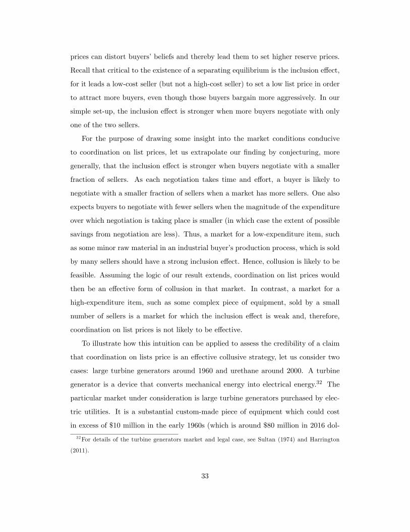
where its dependence on q is made explicit.31 For (α, β) ∈ [0, 1] × [0, 2], Figure 2

reports the maximum welfare difference,

∆(α, β) ≡ max{

∆ (q) : q ∈[q (α, β) , q (α, β)

]},

and the minimum welfare difference,

∆(α, β) ≡ min{

∆ (q) : q ∈[q (α, β) , q (α, β)

]}.

Figure 2 shows that ∆(α, β) > 0 for most values of (α, β) so collusion improves

welfare for some values of q. In addition, for some values of (α, β), ∆(α, β) > 0 so

welfare is higher under collusion for all values of q (for which collusion is feasible and

profitable). By reducing the aggressiveness of buyers, collusion enhances the total

surplus in the market by resulting in more Pareto-improving transactions and that

31 In the Online Appendix, the expression for ∆ (q) is provided.

31

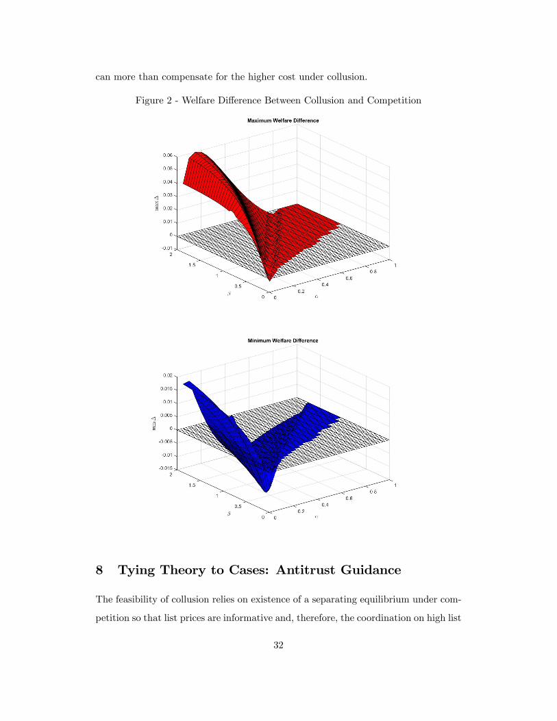
can more than compensate for the higher cost under collusion.

Figure 2 - Welfare Difference Between Collusion and Competition

8 Tying Theory to Cases: Antitrust Guidance

The feasibility of collusion relies on existence of a separating equilibrium under com-

petition so that list prices are informative and, therefore, the coordination on high list

32

prices can distort buyers’beliefs and thereby lead them to set higher reserve prices.

Recall that critical to the existence of a separating equilibrium is the inclusion effect,

for it leads a low-cost seller (but not a high-cost seller) to set a low list price in order

to attract more buyers, even though those buyers bargain more aggressively. In our

simple set-up, the inclusion effect is stronger when more buyers negotiate with only

one of the two sellers.

For the purpose of drawing some insight into the market conditions conducive

to coordination on list prices, let us extrapolate our finding by conjecturing, more

generally, that the inclusion effect is stronger when buyers negotiate with a smaller

fraction of sellers. As each negotiation takes time and effort, a buyer is likely to

negotiate with a smaller fraction of sellers when a market has more sellers. One also

expects buyers to negotiate with fewer sellers when the magnitude of the expenditure

over which negotiation is taking place is smaller (in which case the extent of possible

savings from negotiation are less). Thus, a market for a low-expenditure item, such

as some minor raw material in an industrial buyer’s production process, which is sold

by many sellers should have a strong inclusion effect. Hence, collusion is likely to be

feasible. Assuming the logic of our result extends, coordination on list prices would

then be an effective form of collusion in that market. In contrast, a market for a

high-expenditure item, such as some complex piece of equipment, sold by a small

number of sellers is a market for which the inclusion effect is weak and, therefore,

coordination on list prices is not likely to be effective.

To illustrate how this intuition can be applied to assess the credibility of a claim

that coordination on lists price is an effective collusive strategy, let us consider two

cases: large turbine generators around 1960 and urethane around 2000. A turbine

generator is a device that converts mechanical energy into electrical energy.32 The

particular market under consideration is large turbine generators purchased by elec-

tric utilities. It is a substantial custom-made piece of equipment which could cost

in excess of $10 million in the early 1960s (which is around $80 million in 2016 dol-

32For details of the turbine generators market and legal case, see Sultan (1974) and Harrington

(2011).

33

lars). At the time, General Electric and Westinghouse were the only producers of

turbine generators. In light of the item’s high expense to a buyer and the presence of

only two sellers, it is quite likely that a buyer would negotiate with both sellers. In

such a market, our theory suggests that list prices would be uninformative because

most buyers would negotiate with both sellers. Therefore, coordinating on list prices

would be an ineffective method of collusion because a seller’s list price would have

little effect on a buyer’s beliefs about a seller’s cost and thus have minimal impact

on bargaining and final transaction prices. While GE and Westinghouse did collude

in this market, it is notable that they did so by first coordinating on a policy of not

offering discounts in which case list prices became actual transaction prices. GE then

acted as a price leader on list prices. Absent a move to a “no negotiation” policy,

the theory of this paper suggests that coordination on list prices would have been

ineffective.

Returning to a case discussed in the Introduction, the urethane market would ap-

pear to have features more conducive to coordination on list prices.33 Polyurethanes

are used in various consumer and industrial products including mattress foams, insu-

lation, sealants, and footwear. BASF, Bayer, Dow Chemical, Huntsman, and Lyon-

dell either pled guilty or were convicted of coordinating their list prices over 2000-03.

Their market shares in the sub-markets for polyether polyols, toluene diisocyanate

(TDI), and methylene diphenyl diisocyanate (MDI) are shown in Figure 3. In contrast

to turbine generators with two sellers, buyers of various categories of polyurethane

had four or five suppliers from which to choose.34 While, at present, we do not

have any data on the level of expenditure for a buyer, it is probably not a big ticket

item like a large turbine generator. It would then seem unlikely that a buyer would

negotiate with all or almost all sellers. If that is so then the inclusion effect might

be significant enough to support informative list prices which would be the basis for

33The enusing facts are from In re: Urethane Antitrust Litigation, 768. F.3d 1245 (10th Cir. 2014)

and Class Plaintiffs’Response Brief, In re: Urethane Antitrust Litigation, (10th Cir.), February 14,

2014.34Cartel members controlled the entire market for MDI and TDI and 79% of the market for

polyether polyols.

34

firms effectively colluding by coordinating their list prices.

Figure 3: Market Shares in Urethane

Source: Class Plaintiffs’Response Brief,

In re: Urethane Antitrust Litigation, (10th Cir.), February 14, 2014

9 Concluding Remarks

The primary contribution of this paper is to show that coordination on list prices

can be an effective form of collusion even though firms are left unconstrained in the

final prices they offer buyers. By coordinating on high list prices, sellers can cause

buyers to believe that costs are likely to be high which will induce buyers to bargain

less aggressively and that will serve to raise final negotiated prices. Notably, sellers

continue to bargain in a competitive manner. We also offer some initial insight for

what types of markets are suitable for this type of collusive practice.

In concluding, we offer two directions for future research. The model assumed

that buyers live for only one period and lack information prior to their arrival in

the market. This assumption was made for purposes of tractability in order to focus

on the phenomenon of coordination on list prices. Of course, industrial buyers live

for many periods which then means there is a game between buyers and sellers.

Buyers use data over time to assess whether firms are colluding, and sellers (if they

are colluding) adjust their behavior in order to balance higher profits earned from

35

collusion against buyers becoming more confident that there is collusion. The latter

is detrimental to a cartel because it means buyers will negotiate more aggressively if

they think high list prices are less likely to signal high cost, and there is the possibility

that buyers may pursue private litigation to claim damages. There is no research that

models equilibrium behavior in a dynamic game in which colluding sellers try to avoid

detection and buyers try to detect collusion. While technically challenging, it is a

research direction that is likely to shed new light on cartel pricing dynamics.35

A natural question is why firms would choose to coordinate only on list prices

rather than go that additional step and coordinate on final prices, especially given that

express communication on either list or final prices is per se illegal. The answer may

lie with a cartel’s concern about detection. For two reasons, detection by customers or

the competition authority may be less likely when firms only coordinate on list prices.

First, coordinating on final prices along with a market allocation (and the monitoring

of sales) requires more extensive and frequent communication among cartel members

which enhances the chances of the cartel’s discovery. Second, customers might be less

inclined to think that firms are colluding when they offer different final prices, even

though their list prices are similar. Competition in final prices could make buyers

less inclined to suspect collusion. A topic for future research is to understand when

firms prefer to coordinate on final prices and when they instead prefer to coordinate

only on list prices.

35Besanko and Spulber (1990) consider a static game of incomplete information between a (possi-

ble) cartel and customers who are trying to determine whether there is a cartel. Harrington (2004,

2005) and Harrington and Chen (2006) examine the impact of detection for the price path in a

dynamic setting but customers are represented by a detection technology and thus are not strategic.

36

10 Appendix

Proof of Lemmas 1 and 2: First, it can be verified that given hL(c) > hH(c), we

have hL(c) > hκ(c) > hH(c) if κ ∈ (0, 1).

To show Lemma 1, the first-order conditions of (4) and (6) are given by

v −R1m1m2(v) = hL(R1m1m2

(v)), ∀ (m1,m2) ∈ {(l, l), (l, h) , (h, l)}

v −R1hh(v) = hκ(R1hh(v))

It is easily verified that

R1′m1m2(v) =

1

1 + h′L(R1′m1m2(v))

> 0, ∀ (m1,m2) ∈ {(l, l), (l, h) , (h, l)}

So R1m1m2(v) is increasing in v, ∀ (m1,m2) ∈ {(l, l), (l, h) , (h, l)}.

To show that R1hh(v) > R1ll(v)(= R1lh(v) = R1hl(v)) ∀v, suppose the negation so

that R1hh(v) ≤ R1ll(v) for some v. It follows that

0 ≤ −(R1hh (v)−R1ll (v)

)= hκ(R1hh (v))−hL(R1ll (v)) ≤ hκ(R1hh (v))−hL(R1hh (v)) < 0

which is a contradiction.

Next to show Lemma 2, when (m1,m2) ∈ {(l, l), (h, h)}, the first-order condition

from (5) and (7) are given by

v −R2ll(v) = hL(R2ll(v)) (32)

v −R2hh(v) = hκ(R2hh(v)) (33)

So we have R2ll(v) = R1ll(v) and R2hh(v) = R1hh(v). When (m1,m2) ∈ {(l, h), (h, l)},

say, when (m1,m2) = (l, h), the first-order condition from (5) becomes

0 =(1− FH(R2lh)

)fL(R2lh)

[(v −R2lh

)− hL

(R2lh)]

+(1− FL(R2lh)

)fH(R2lh)

[(v −R2lh

)− hH

(R2lh)].

Given the assumption that hL(R2lh)> hH

(R2lh), we have(

v −R2lh)− hL

(R2lh)< 0 <

(v −R2lh

)− hH

(R2lh), (34)

37

As(v −R2ll

)− hL

(R2ll)

= 0 (from (32)) then (34) implies(v −R2lh

)− hL

(R2lh)<(

v −R2ll)− hL

(R2ll). As

(v −R2hh

)− hκ

(R2hh

)= 0 (from (33)) then (34) implies(

v −R2hh)− hκ

(R2hh

)<(v −R2lh

)− hH

(R2lh). Those two conditions imply R2lh +

hL(R2lh)> R2ll+hL

(R2ll)and R2hh+hκ

(R2hh

)> R2lh+hH

(R2lh). When κ is suffi ciently

small, we have R2hh + hκ(R2hh

)> R2hh + hH

(R2hh

)> R2lh + hH

(R2lh)by continuity of

hκ(R2hh

)in κ.

Given that h′t(z) > 0, we have the strict monotonicity of z + ht(z), t ∈ {L,H}.

Thus ∃κ > 0 such that if κ ∈ [0, κ] then R2hh (v) > R2lh (v) > R2ll (v) ,∀v.

38

References

[1] Awaya, Yu and Vijay Krishna, “On Communication and Collusion,”American

Economic Review, 106 (2016), 285-315.

[2] Besanko, David and Daniel F. Spulber, “Antitrust Enforcement under Asym-

metric Information,”Economic Journal, 99 (1989), 408-425.

[3] Besanko, David and Daniel F. Spulber, “Are Treble Damages Neutral? Se-

quential Equilibrium and Private Antitrust Enforcement,”American Economic

Review, 80 (1990), 870-887.

[4] Chan, Jimmy and Wenzhang Zhang, “Collusion Enforcement with Private In-

formation and Private Monitoring,” Journal of Economic Theory, 157 (2015),

188-211.

[5] Chen, Yongmin and Robert W. Rosenthal, “Asking Prices as Commitment De-

vices,”International Economic Review, 37 (1996), 129-155.

[6] Connor, John M., Global Price Fixing, 2nd Edition, Berlin: Springer, 2008.

[7] Connor, John M. and Robert H. Lande, “Not Treble Damages: Cartel Recoveries

Are Mostly Less Than Single Damages,” Iowa Law Review, 100 (2015), 1997-

2023.

[8] Crawford, Vincent P. and Joel Sobel, “Strategic Information Transmission,”

Econometrica, 50 (1982), 1431-1451.

[9] Farrell, Joseph and Robert Gibbons, “Cheap Talk Can Matter in Bargaining,”

Journal of Economic Theory, 48 (1989), 221-237.

[10] García Díaz, Antón, Roberto Hernán González, and Praveen Kujal, “List Pricing

and Discounting in a Bertrand-Edgeworth Duopoly,” International Journal of

Industrial Organization, 27 (2009), 719-727.

[11] Gill, David and John Thanassoulis, “Competition in Posted Prices with Stochas-

tic Discounts,”Economic Journal, 126 (2016) 1528-1570.

39

[12] Harrington, Joseph E., Jr., “Noncooperative Behavior by a Cartel as an Entry-

Deterring Signal,”Rand Journal of Economics, 15 (1984), 426-433.

[13] Harrington, Joseph E., Jr., “Cartel Pricing Dynamics in the Presence of an

Antitrust Authority,”RAND Journal of Economics, 35 (2004), 651-673.

[14] Harrington, Joseph E., Jr., “Optimal Cartel Pricing in the Presence of an An-

titrust Authority,”International Economic Review, 46 (2005), 145-169.

[15] Harrington, Joseph E. Jr., “How Do Cartels Operate?,”Foundations and Trends

in Microeconomics, Vol. 2, Issue 1, July 2006.

[16] Harrington, Joseph E. Jr., “Posted Pricing as a Plus Factor,”Journal of Com-

petition Law and Economics, 7 (2011), 1-35.

[17] Harrington, Joseph E., Jr. and Myong-Hun Chang, “Modelling the Birth and

Death of Cartels with an Application to Evaluating Antitrust Policy,”Journal

of the European Economic Association, 7 (2009), 1400-1435.

[18] Harrington, Joseph E., Jr. and Myong-Hun Chang, “When Should We Expect a

Corporate Leniency Program to Result in Fewer Cartels?,”Journal of Law and

Economics, 28 (2015), 417-449.

[19] Harrington, Joseph E., Jr. and Joe Chen, “Cartel Pricing Dynamics with Cost

Variability and Endogenous Buyer Detection,” International Journal of Indus-

trial Organization, 24 (2006), 1185-1212.

[20] Harrington, Joseph E., Jr. and Andrzej Skrzypacz, “Private Monitoring and

Communication in Cartels: Explaining Recent Collusive Practices,”American

Economic Review, 101 (2011), 2425-2449.

[21] Harrington, Joseph E. Jr. and Yanhao Wei, “What Can the Duration of Discov-

ered Cartels Tell Us About the Duration of All Cartels?,”University of Penn-

sylvania, working paper, December 2015 (Economic Journal, forthcoming).

40

[22] Hay, George A. and Daniel Kelley, “An Empirical Survey of Price Fixing Con-

spiracies,”Journal of Law and Economics, 17 (1974), 13-38.

[23] Holmes, William C., Antitrust Law Handbook, West Group, 2005.

[24] Kim, Kyungmin and Philipp Kircher, “Effi cient Competition through Cheap

Talk: The Case of Competing Auctions,” University of Iowa, working paper,

December 2014.

[25] LaCasse, Chantale, “Bid Rigging and the Threat of Government Prosecution,”

RAND Journal of Economics, 26 (1995), 398-417.

[26] Lester, Benjamin, Ludo Visschers, and Ronald Wolthoff, “Competing with Ask-

ing Prices,”Federal Reserve Bank of Philadelphia, working paper, May 2015.

[27] Levenstein, Margaret C. and Valerie Y. Suslow, “What Determines Cartel Suc-

cess?,”Journal of Economic Literature,, 44 (2006), 43-95.

[28] Marshall, Robert C. and Leslie M. Marx, The Economics of Collusion - Cartels

and Bidding Rings, Cambridge, Mass.: The MIT Press, 2012.

[29] Menzio, Guido, “A Theory of Partially Directed Search,” Journal of Political

Economy, 115 (2007), 748-769.

[30] Quint, Daniel and Kenneth Hendricks, “Indicative Bidding in Auctions with

Costly Bidding,”University of Wisconsin, working paper, September 2015.

[31] Raskovich, Alexander, “Competition or Collusion? Negotiating Discounts off

Posted Prices,”International Journal of Industrial Organization, 25 (2007), 341-

354.

[32] Rotemberg, Julio J. and Garth Saloner (1986). “A Supergame-Theoretic Model

of Price Wars During Booms.”American Economic Review, 76, 390-407.

[33] Schinkel, Maarten Pieter and Jan Tuinstra, “Imperfect Competition Law En-

forcement,” International Journal of Industrial Organization, 24 (2006), 1267—

1297.

41

[34] Souam, Saïd, “Optimal Antitrust Policy under Different Regimes of Fines,”In-

ternational Journal of Industrial Organization, 19 (2001), 1-26.

[35] Spector, David, “Facilitating Collusion by Exchanging Non-verifiable Sales Re-

ports,”Paris School of Economics, February 2015.

[36] Sugaya, Takuo and Alexander Wolitzky, “Maintaining Privacy in Cartels,”Stan-

ford University, July 2016.

[37] Sultan, Ralph G. M., Pricing in the Electrical Oligopoly, Vol. I, Cambridge,

Mass.: Harvard University Press, 1974.

[38] Ye, Lixin, “Indicative Bidding and a Theory of Two-Stage Auctions,”Games

and Economic Behavior, 58 (2007), 181-207.

42