Embed Size (px)
Citation preview
Coordination and Flexibility in Supply Contracts with Options
Dawn Barnes–Schuster*
Rotelsteig 9, CH-8037 Zurich
Yehuda Bassoky
Marshall School of Business
University of Southern California, Los Angeles, CA 90089
Ravi Anupindiz
Stern School of Business
New York University, New York, NY 10012
First version: February 28, 1998
Second version: May 12, 1999
Third version: March 8, 2000
Last revised: March 11, 2002
*Email: [email protected]; Phone: 41-1-364-5085yEmail: [email protected]; Phone: (213)821-1140zEmail: [email protected]; Phone: (212)998-0487

Coordination and Flexibility in Supply Contracts with Options
Abstract
We investigate the role of options (contingent claims) in a buyer-supplier system. Specif-
ically using a two-period model with correlated demand, we illustrate how options provide
flexibility to a buyer to respond to market changes in the second period. We also study the
implications of such arrangements between a buyer and a supplier for coordination of the
channel. We show that, in general, channel coordination can be achieved only if we allow the
exercise price to be piecewise linear. We develop sufficient conditions on the cost parameters
such that linear prices coordinate the channel. We derive the appropriate prices for chan-
nel coordination which, however, violate the individual rationality constraint for the supplier.
Contrary to popular belief (based on simpler models) we show that credit for returns offered
by the supplier do not always coordinate the channel and alleviate the individual rationality
constraint. They are are useful only on a subset of the feasibility region under which channel
coordination is achievable with linear prices. Finally, we demonstrate (numerically) the ben-
efits of options in improving channel performance and evaluate the magnitude of loss due to
lack of coordination.

March 11, 2002 Supply Contracts with Options
1 Introduction
In recent years, it has become widely recognized that to compete effectively firms need to
develop the capability to respond quickly to changing market needs. For example, consider
a simple single-supplier single-buyer system operating in a market with short product life
cycles and highly unpredictable demands. In such situations flexibility for a buyer implies
the ability to get additional products in response to changes in market demands during the
short life cycle of the product. While this flexibility benefits the buyer, it may come at some
cost to the supplier.1 Therefore, a supplier will usually provide limited flexibility or may offer
prices based on the level of flexibility desired by the buyer. We illustrate some practices from
three different industries, viz. toys, apparel, and electronics.
Consider the following situation recently faced by the toy maker Mattel, Inc. (Kravetz,
1999):
Mattel was hurt last year by inventory cutbacks at Toys “R” Us, and officials are also eager
to avoid a repeat of the 1998 Thanksgiving weekend. Mattel had expected to ship a lot of
merchandise after the weekend, but retailers, wary of excess inventory, stopped ordering
from Mattel. That led the company to report a $500 million sales shortfall in the last
weeks of the year . . . For the crucial holiday selling season this year, Mattel said it will
require retailers to place their full orders before Thanksgiving. And, for the first time,
the company will no longer take reorders in December, Ms. Barad said. This will enable
Mattel to tailor production more closely to demand and avoid building inventory for orders
that don’t come.
Effectively, Mattel is deciding not to provide any flexibility to its retailers to respond to
in-season changes in market demand. While this strategy limits the downside risk for Mattel,
the upside potential is also limited. The basic premise of this paper is that such measures
may hurt overall channel performance. While providing flexibility is costly (e.g., inventory
carrying for Mattel), mechanisms exist to mitigate this risk and create a win-win situation
for both the manufacturer and the retailer.
The apparel industry is plagued by the increasing cost of markdowns (Frazier, 1986; Ham-
mond, 1990; Fisher, Hammond, Obermeyer & Raman, 1994) running into billions of dollars.
A primary reason for this phenomenon is that retailers must place firm, SKU-specific orders1The additional cost is incurred due to some inflexibility a supplier faces; e.g., long production lead-times or long
procurement lead-times for some component(s) that the supplier uses in her production process. Consequently,
to provide the flexibility to a buyer, she may carry additional inventory of raw material or finished goods, and/or
employ expediting or out-source production, all of which entail additional costs.
1

March 11, 2002 Supply Contracts with Options
well in advance of the beginning of the selling season (Nuttle, Hunter & King, 1991) despite
demonstrable advantages to in-season replenishment (Whalen, 1993; King & Hunter, 1996;
Hunter, King & Nuttle, 1996; Pinnow & King, 1997). These studies estimate that the sav-
ings to the retailer are large enough that he/she can afford to pay an additional 30%-50%
to a supplier that provides in-season replenishments. In-season replenishments are prob-
lematic due to long procurement/production lead times for manufacturers when compared to
the length of the selling season faced by a retailer.2 A manufacturer can make in-season re-
plenishment possible either by reducing the lead time or by carrying inventories. The latter
strategy of carrying (raw-material or finished goods) inventories, however, comes with risks
of over-stocking. The industry has undertaken several efforts to reduce the lead time; yet, ap-
parently these have not been sufficient to facilitate in-season replenishments as documented
by the studies mentioned earlier.
In the apparel catalog industry, contracts similar to ours have been used to provide flexibil-
ity to a buyer for in-season replenishment. Under a backup agreement (Eppen & Iyer, 1997),
a buyer commits to a total order quantity for the season. A prespecified fraction of the total
quantity is delivered initially. The buyer may purchase additional units up to the remaining
commitment at a later date. He pays a penalty for any committed units not purchased. Such
contracts are used, for example, by Anne Klein, Finity, DKNY, and Liz Claiborne with the
catalog company Catco (Eppen & Iyer, 1997).
Finally, in the electronics industry, flexibility for reorders is provided under arrangements
known as quantity-flexibility contracts. Under such an arrangement, the buyer first provides
a forecast of future orders to the supplier. In subsequent periods, he is allowed to place actual
orders which are within prespecified limits of the original forecasts; in addition, he may be
allowed to update the future forecasts. Such contracts are used, for example, by IBM Printer
Division (Bassok, Srinivasan, Bixby & Wiesel, 1997), Sun Microsystems (Farlow, Schmidt &
Tsay, 1995), Solectron, Hewlett Packard, etc. (Tsay & Lovejoy, 1999). In the semiconductor
industry, under agreements called pay-to-delay capacity reservation, allocation and reserva-
tion for wafer fabrication capacity is offered by a supplier in return for a fixed up-front pay-
ment (Brown & Lee, 1997). The buyer could then place orders at a later date and use the
up-front payment towards actual procurement costs. A large portion of the allocation is usu-2Lovejoy (1999) states that this lead time consists of the long production lead-time of the fabric (estimated
to be larger than 10 weeks) and the transportation lead time from off-shore production facilities (4 weeks). He
argues that the apparel production itself is relatively fast and takes between 2 and 7 days. The length of the
selling season is between 20-24 weeks. Even if we assume that new orders will be placed only four periods into
the season these orders will arrive only towards the end of the season, and will not be of great help.
2

March 11, 2002 Supply Contracts with Options
ally “take-or-pay” capacity, capacity for which the manufacturer will have to pay the full wafer
production price even if he does not need the wafers. Brown and Lee (1997) state that accord-
ing to a recent survey by the Fabless Semiconductor Association, 30% of capacity reservation
arrangements are pure take-or-pay. Recently, however, options for capacity have been offered
by the Taiwanese Semiconductor Manufacturing Company (Chang, 1996), a semiconductor
fabrication foundry company.
In a supply chain context, in addition to the need for a provision of flexibility, the abil-
ity to “coordinate” decisions between various links in the chain becomes critical (Hammond,
1992). When the buyer and the supplier optimize their respective objective functions, ‘double
marginalization’ (Tirole, 1990) adversely impacts channel performance. Several policies have
been proposed for channel coordination, notable among which are non-linear prices (e.g, a
two-part tariff, quantity discounts) and return policies.
In this paper we provide a generic framework for the study of the role of options in a
buyer-supplier system for short life cycle products. We show that backup agreements, two-
period quantity flexibility contracts, and pay-to-delay arrangements are but special cases. We
then illustrate how options provide flexibility to a buyer to respond to market changes and
study the implications of such arrangements between a buyer and a supplier for coordination
of the system. In developing a model for the supply chain, we focus particularly on the apparel
industry.
Consider a single-buyer single-supplier system. The buyer sells a single product to con-
sumers at a fixed market price that is exogenously specified. The product life cycle is short;
we refer to this short life cycle as a season and assume it to be of fixed duration. We divide
the season into two periods of possibly unequal lengths with correlated demands. The buyer
updates the second period demand and places an additional order after observing and satis-
fying actual first period demand.3 Before the beginning of the horizon the buyer makes three
decisions. He places firm orders for goods to be delivered at the beginning of periods one and
two. In addition, he purchases options from the supplier which give him an opportunity to
order additional units of the product (up to the number of options purchased) before the start
of period two but after observing demand in period one. The total procurement costs consist
of the following components: (i) unit wholesale prices for goods procured against firm orders
in each period, (ii) an option price for every unit of option purchased, and (iii) an exercise price3Fisher and Raman (1996) have documented the value of updating the forecast after initial sales (e.g., 20%
into the season) are observed. Eppen and Iyer (1997) also state that the demand update occurs fairly early in the
season thus justifying the unequal lengths for the two periods.
3
March 11, 2002 Supply Contracts with Options
for options exercised to obtain additional products in the second period. Excess demand is
back-ordered in the first period and is considered lost sales in the second period. The buyer
incurs the standard holding and penalty costs and earns revenues for the products sold for
the two periods.
To produce the goods for the buyer, the supplier procures components / raw materials
from its upstream supplier that require a long lead-time such that there is no opportunity to
reorder these during the season. Furthermore, the raw material is costly and so the supplier
is unwilling to take the risk of carrying it unless the buyer is willing to share this risk. We
believe this accurately reflects the situation in the apparel industry described earlier where
the supplier is the apparel manufacturer and the buyer is the retailer. For the firm orders
that a buyer places, the supplier can purchase the exact quantities of raw material needed.
There is some uncertainty, however, regarding the number of additional units of the good a
buyer may need in the second period. To be able to provide flexibility to the buyer to order
additional goods, the supplier needs to procure sufficient raw material in advance with the
associated risks. To mitigate this risk, she offers options to the buyer at a price. The supplier
makes a commitment to produce products for the second period, up to the number of options
purchased by the buyer. The supplier has two production opportunities. She can produce at
a regular (cheaper) cost before and during the first period. In addition, at an extra cost, she
can also produce before the beginning of the second period but after observing the number
of options exercised by the buyer. The supplier needs to determine the optimal wholesale,
option, and exercise prices, and in addition determine the optimal production quantities for
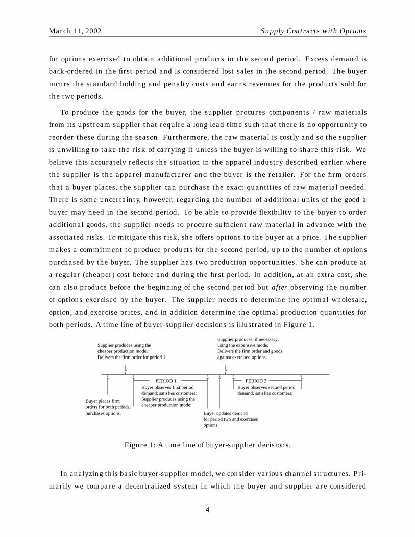
both periods. A time line of buyer-supplier decisions is illustrated in Figure 1.
Supplier produces using thecheaper production mode;
orders for both periods;purchases options.
Buyer places firm
Buyer updates demandfor period two and exercisesoptions.
Supplier produces using thecheaper production mode;
Delivers the firm order for period 1.
PERIOD 1
demand; satisfies customers;
Delivers the firm order and goodsagainst exercised options.
PERIOD 2Buyer observes first period Buyer observes second period
demand; satisfies customers;
Supplier produces, if necessary;using the expensive mode;
Figure 1: A time line of buyer-supplier decisions.
In analyzing this basic buyer-supplier model, we consider various channel structures. Pri-
marily we compare a decentralized system in which the buyer and supplier are considered
4
March 11, 2002 Supply Contracts with Options
independent profit maximizers to a centrally controlled channel. We then ask: can chan-
nel coordination be achieved? Channel Coordination is achieved when the supplier and the
buyer make decisions (independently) in such a way that the joint profits are maximized.
In addition, to compare the performance of the systems with options we use a benchmark
decentralized model in which no options are offered.
In highlighting our contributions, it is useful to first understand what has been accom-
plished in the literature. Observe that the two key elements of our model include (i) options
as an instrument of flexibility and (ii) incentives for coordination in such environments. Sev-
eral researchers have considered options or option-like arrangements for flexibility provided
through a supply contract. Most of this research, however, takes a single-decision maker
approach and derives the optimal policy for the buyer under a given contract. For exam-
ple, in a two-period problem with correlated demands, Eppen and Iyer (1997) study backup
agreements and Brown and Lee (1997) study pay-to-delay capacity reservation contracts. In
a multi-period setting with uncorrelated demands Bassok and Anupindi (1998) and Tsay and
Lovejoy (1999) study quantity-flexibility contracts.
Some of the key insights developed by these papers include (i) flexibility required increases
with the coefficient of variation (CV) of demand (Bassok & Anupindi, 1998; Tsay & Lovejoy,
1999), and (ii) value of flexibility (through backup or pay-to-delay contracts) is based more on
the ability to learn from early demand than on CV of demand (Eppen & Iyer, 1997; Brown
& Lee, 1997). Some questions remain. For example, do these relationships hold up in equi-
librium? When are such contracts efficient (i.e., coordinate the channel)? We show that, in
equilibrium, the value of flexibility (through option contracts in our case) depends both on
the CV of demand and the correlation coefficient. In fact, there is a “complementarity” re-
lationship between the two. That is, the increase in the value of flexibility with correlation
increases with the CV of demand. Furthermore, we develop sufficient conditions under which
backup agreements are efficient.
The second key element of our study includes incentives for channel coordination. There
is a large body of literature that studies incentive contracts for channel coordination un-
der stochastic demand; see for example, Pasternack (1985), Donohue (1996), Ernst and Co-
hen (1992), Moses and Seshadri (2000), Tsay (1999), Narayanan and Raman (1997), Kouvelis
and Gutierrez (1997), Iyer and Bergen (1997), Cachon and Lariviere (1997), and Lee and
Whang (1999). Clearly, channel coordination is always achieved when the buyer is able to
internalize the costs of the supplier. This happens, for example, if the supplier “sells the firm”
to the buyer, implemented by a supplier charging marginal costs. There are two issues with
5

March 11, 2002 Supply Contracts with Options
this approach. First, marginal cost pricing may not be linear. So if a firm is restricted to
linear pricing, can channel coordination still be achieved? We develop sufficient conditions
under which this is possible. Second, marginal cost pricing is not individually rational for
the supplier. Hence extant research has focused on individually rational instruments for
coordination; for example, return policies and non-linear prices. This paper enhances our
understanding of such instruments for coordination which we now briefly elaborate.
The role of return policies (also called buy-backs) to achieve channel coordination was
established by Pasternack (1985) for single period models under the assumption of identical
salvage values for both the manufacturer and the buyer and frictionless implementation of
return policies.4 Donohue (1996) extends this to a two-period setting that includes options. In
her model the supplier must preposition some portion of component inventory before demand
information is known, entailing a risk that is shared via options. Our model differs from hers
in several ways. While she limits her model to goods purchased entirely using options, we
allow both committed orders and options. Moreover, in her model, while information may be
revealed in two stages, demand is realized only once, and hence the model itself remains that
of a single period like in Pasternack (1985). Thus these models do not accurately capture the
phenomenon of in-season replenishments. In contrast, in our setting early information comes
from actual observed demand leading to a two period model. Furthermore, her analysis is
restricted to the case of perfect correlation while we present results for general correlation
structures. Finally, like Pasternack (1985) she assumes identical salvage values for the buyer
and the supplier and a frictionless returns process, while we make no such assumptions.
Not surprisingly, the key findings of Pasternack (1985) and Donohue (1996) are similar;
namely, (i) return policies coordinate the channel and (ii) credit for returns allows an arbi-
trary spread of the channel profits between the buyer and the supplier (Donohue illustrates
this under perfect correlation of demand). Several questions remain. What happens when
their cost assumptions do not hold? Can return policies still coordinate the channel? Can
return policies achieve an arbitrary split of channel profits under more general conditions?
Our results show that return policies do not always coordinate the channel. We develop cost
conditions under which coordination is achieved (which includes the assumptions made by
Pasternack and Donohue). When the channel is coordinated, however, credit for returns does
achieve an arbitrary split of channel profits for any correlation thus generalizing the result of
Donohue.
Finally, using an extensive numerical study, we attempt to characterize environments, pro-4A frictionless returns process implies that there is no cost to either party to execute the returns process.
6

March 11, 2002 Supply Contracts with Options
viding managerial insights, under which (i) benefits of options and coordination are large, (ii)
options alone capture most of these benefits, and (iii) incentives for coordination, in addition,
are desirable.
The rest of the paper is organized as follows. In section 2 we first present a general model
encompassing the various flexibility arrangements discussed earlier as special cases. We also
describe the various channel structures and the model assumptions here. Subsequently in
section 3 we develop expressions for the expected profit of the buyer and the supplier for vari-
ous channel structures. In section 4 we discuss the issue of channel coordination under linear
prices. In section 5, we numerically compare the performance of various channel structures.
We conclude in section 6. We give expressions for the profit functions in Appendix A. Proofs
of all results are available from the authors upon request.
2 A General Model
We consider a single-buyer single-supplier system with two periods and correlated demands.
The buyer makes three ordering decisions at the beginning of the horizon. First, he orders
Qi units at a unit wholesale price of ci to be delivered at the beginning of period i 2 f1; 2g;
we refer to the Qi as firm orders.5 In addition, he purchases M options at a unit option price
of co. In period two, he may choose to exercise m � M options at a per unit exercise price
of ce. We assume that one option gives the buyer a right to purchase one unit of good. The
buyer sells goods to the consumer at a unit price of r. Let hbi and pi be the unit holding and
shortage penalty cost for period i 2 f1; 2g. The holding costs for the two periods are permitted
to differ in order to account for possible disparity in period lengths. The shortage costs differ
reflecting the difference between a loss of goodwill due to backlogging of excess demand in
the first period and the cost associated with not satisfying a customer at all (lost sale) in the
second period. Any leftover finished goods at the end of the second period may be salvaged
at a per unit price of ~vbf . We define the effective salvage value of finished goods for the buyer
to be vbf = ~vbf � hb2. Demand in period i 2 f1; 2g, denoted by Di, is assumed to be normally
distributed with mean �i and standard deviation �i with conditional density and distribution
functions of fDi(�) and FDi
(�) respectively. Demands in the two periods are correlated with
a correlation coefficient of �. Throughout the paper we will use uppercase Di to denote the5Observe that the second firm order Q2 does play an important role. Even though he decides Q2 at the begin-
ning of the horizon, the buyer saves holding cost on finished goods by asking for delivery later during the season.
This allows the supplier to better manage her production capacity. In addition, using Q2 she may increase the
average number of products sold using the cheaper mode of production.
7

March 11, 2002 Supply Contracts with Options
demand random variable and lowercase di to denote a realization of the appropriate demand
random variable. The standard normal distribution function is denoted by �(�).
The supplier must purchase sufficient raw material to produce the maximal quantity pos-
sibly requested (that is, Q1 + Q2 +M , the sum of the committed orders and the options pur-
chased).6 The per unit procurement cost of raw material is cr. As discussed earlier, the
supplier has two modes of production. She will produce the required quantity (Q1) for the
first period using the cheaper production mode at a unit labor cost of cL. In addition, she may
choose to produce the firm requirements for the second period (Q2) and any extra production
that she desires (in anticipation of high demand in the second period) using the cheaper pro-
duction mode (before or during the first period) and thus incur a per unit holding cost of hs.
Let XL be the total units produced using the cheaper production mode. In the second period,
after the buyer exercises options, the supplier may undertake additional production using an
expensive production mode. We assume that additional production is expensive due to in-
creased labor costs (for example, due to overtime costs and/or disruptions of other scheduled
work); specifically the supplier incurs a total labor cost of cL(1 + ) where is an exogenous
parameter. We assume that the capacity in both production modes is sufficient to produce
any quantity up to the number of options purchased by the buyer.7 Any raw material left
over after supplying the goods needed against options exercised by the buyer is immediately
salvaged for vsr per unit. Hence, the supplier does not hold any raw material inventory in the
second period. We do not explicitly account for raw material holding cost in the first period.
Whether or not the supplier incurs this cost depends on how the raw material is delivered. If
raw material is staged for delivery just-in-time for the two production opportunities then the
supplier does not incur any holding cost in the first period. Alternately, all raw material may
be delivered to the supplier in the first period. In such cases, any first period raw material
holding cost can be incorporated into the expedited second period production cost and salvage
value of the raw material. Any leftover finished goods are also immediately salvaged (at the
beginning of second period, after satisfying exercised options) for vsf per unit. Since capacity
is unconstrained, the supplier will be able to produce exactly what the buyer requests, and
hence experiences no shortage cost.6We implicitly assume that the raw material has a long acquisition lead time such that it needs to be processed
before the start of the season. The supplier can, however, acquire any amount of raw material.7That is, the bottleneck in the supply chain is raw material/component procurement. Once the buyer pur-
chases options, the maximum production quantity of apparel is known to the manufacturer who can then plan
appropriate capacity.
8

March 11, 2002 Supply Contracts with Options
2.1 Special Cases
We now demonstrate that the various flexibility contracts presented in the section 1 are spe-
cial cases of our general model.
Backup Agreement
In a model of a backup agreement presented in Eppen and Iyer (1997), the buyer, at the
beginning of the season, makes a firm commitment to purchase Q units during the season.
At the first period she purchases Q1 = Q(1 � �) units, at the price c per unit. At the second
period the buyer may purchase up to Q� units at the price c per unit. If the buyer decides to
purchase m units in the second period, where m < Q� then she pays a penalty, b per unit, for
the remaining Q� �m units not purchased. The correspondence between our general model
parameters and a backup agreement is shown in Table 1.
Quantity Flexibility (QF) Contract
Consider a two–period version of the commonly used quantity flexibility contract (Bassok
& Anupindi, 1998; Tsay & Lovejoy, 1999). The wholesale price is c for both periods. The
quantities committed for the two periods are ~Q1 and ~Q2. Let the second period upward and
downward flexibility be �u and �d respectively. That is, in the second period the maximum
quantity that can be purchased is ~Q2(1 + �u) and the minimum quantity that needs to be
purchased is ~Q2(1� �d) at the unit price of c. The correspondence between the general model
parameters and a QF contract is shown in Table 1.
Pay-to-Delay Capacity Reservation
Under this form of capacity reservation analyzed by Brown and Lee (1997), a buyer makes
a total reservation z of which he is obligated to purchase at least y < z units (called take-or-
pay). He pays a unit cost cf for the take-or-pay capacity and a unit option cost of co for z � y
units. Additional units up to a maximum z � y can be bought at an extra unit cost of ce.8 As
discussed earlier, their analysis is limited to a single period model in which information about
demand is revealed in two stages. In our general model this corresponds to the second period
problem where the first period demand realization is treated as information about demand.
In that case the correspondence between the general model and pay-to-delay reservation (la-
beled as ‘Single Period Demand’) is as shown in Table 1. Alternately, one could apply the
pay-to-delay capacity reservation agreement to allow for two periods of actual demand. The
correspondence follows analogously as shown in Table 1.8Brown and Lee (1997) allow for additional unreserved units to be purchased at a unit cost of cp > ce + co. In
contrast, in our model, we do not allow for this additional source of supply.
9

March 11, 2002 Supply Contracts with Options
General Model Q1 Q2 M c1 c2 co ce
Backup Agreement Q(1� �) 0 Q� c – b c� b
QF Contract ~Q1 (1� �d) ~Q2 (�d + �u) ~Q2 c c 0 c
Pay-to-Delay – y z � y – cf co ce
(Single Period Demand)Pay-to-Delay y – z � y cf – co ce
(Two Period Demand)
Table 1: Special cases.
Thus for any given backup agreement and simple QF contract there exists a corresponding
option contract with restrictions on the number of options and the option/exercise price. Thus
the performance of the channel and the supplier will be no worse with the more general
options contract we propose. Our model specialized to a capacity investment setting with
single period demand realization is equivalent to a pay-to-delay arrangement presented in
Brown and Lee (1997).9 We now proceed with the analysis of the general model proposed in
this paper.
2.2 Channel Structures and Assumptions
We compare three channel structures: In the Centralized System (CS), we assume that there
is one decision maker who controls the channel and hence makes decisions to optimize total
system profits. Observe that under this scenario, the wholesale, option and exercise prices
play no role in determining the system profits. The only appropriate decision variables are
production decisions for the two periods under the two production modes, the shipment quan-
tities, and the quantity of raw material to be ordered at the beginning of the season. The
optimal solution to the CS is called the first-best solution. In the Decentralized System (DS)
system, the buyer and supplier play a Stackelberg game where the supplier is the leader
and the buyer the follower. This is reasonable whenever the supplier has more power in the
channel than the buyer.10 In this situation, for a given set of prices – wholesale, option, and
exercise – announced by the supplier, the buyer places orders in the two periods which maxi-
mize his expected profits. These orders act as implicit demand functions for the supplier, who
then determines the optimal prices and appropriate production quantities that maximize her9Our analysis, with minor modifications, can be used to study capacity reservation issues as in Brown and
Lee (1997).10The alternate situation of buyer being the leader is also possible and is an area of future research.
10

March 11, 2002 Supply Contracts with Options
profits. A Decentralized System with No Options (DSNO) is similar to the DS but without
options. Since there are no options, the buyer cannot order any additional quantity in the sec-
ond period after observing demand; he places firm orders for the two periods at the beginning
of period one.
The CS is used as a benchmark case to investigate if there exists an appropriate decen-
tralization mechanism (through prices and/or quantities) such that the DS will achieve the
first-best solution. In addition, we use the DSNO as a benchmark case to determine if both
the supplier and the buyer increase their profits from the use of options, and numerically
quantify the benefits of using options. Finally, we make the following assumptions:
1. Cost Assumptions: We assume that the raw material, labor and salvage costs exhibit the
following relationships:
Assumption C1: vsf � cr + cL + hs and vsr � cr
Assumption C2: vbf � cr + cL + hs.
Assumption C3: hs � cL .
Assumption C4: hs < hb1.
Assumptions C1 and C2 ensure that the system profits in the CS are finite. Assumption
C1, in addition, ensures that the supplier’s profits in the DS and DSNO are finite. As-
sumption C3 says that it is never more expensive to produce a unit in the cheaper mode
and incur holding cost than to produce it in the expedited mode. Finally, assumption
C4 states that the buyer’s first period holding cost is larger than that of the supplier.
Assumptions C3 and C4 are reasonable and allow us to limit the analysis to a small
number of permutations of the cost parameters.
2. Correlation Structure: We will assume that � < 1. This allows us to focus on a two-period
problem. If � = 1, we effectively have a single period problem and it can be shown that
channel coordination is always achieved (Barnes-Schuster, Bassok & Anupindi, 2002).
3. Information Structure: Demand distributions are common knowledge. Since the sup-
plier’s profits are affected by the buyer’s order quantities and number of options exer-
cised, she needs to know the distribution of demands in both periods to be able to set
optimal prices.
4. Delivery Commitment:
11

March 11, 2002 Supply Contracts with Options
� The supplier is obligated to supply goods against options purchased. This obliga-
tion is part of the contract since the buyer, by purchasing options, acquires the right
to purchase a certain amount of goods. This assumption is also made by other re-
searchers; e.g., Eppen and Iyer (1997), Donohue (1996), and Brown and Lee (1997).
� All goods against exercised options are delivered immediately.
5. Salvage Location: We initially assume that in the CS any excess finished goods at the
supplier and buyer locations will be salvaged at their respective locations regardless of
the salvage values. In section 4 when we discuss return policies, we allow the CS to
salvage in the most favorable location. This allows us to make a fair comparison of CS
and DS in each of the cases – with and without return policies.
3 Analysis
To analyze the various systems, we first need to develop expressions for the expected profits
in each system. For clarity of exposition, we first derive the individual profit functions of the
supplier and the buyer in the DS and then aggregate appropriately to write the profit function
for the CS.
3.1 Buyer’s Profit Function in the DS
The buyer’s ordering problem can be set up as a two-stage stochastic dynamic program. That
is, first we calculate the optimal policy for exercising options given an initial inventory (on-
hand + on-order), I2 = Q1+Q2� d1, at the beginning of the second period. We then substitute
the resulting function into the two-period total profit function. Let (�)+ denote the positive
part of (�).
Buyer’s Order Policy for Period Two
We first develop the buyer’s last period conditional expected profit function,
�b2(m; I2) = ED2
[rmin(D2; (I2 +m)+) + rmin((d1 �Q1)+; Q2 +m)� cem
�p2(D2 � I2 �m)+ + vbf (I2 +m�D2)+]: (1)
The first term is the buyer’s revenue from current sales, the second term is revenue from
first period backorders satisfied in period two, and the third term is the cost to exercise m
12

March 11, 2002 Supply Contracts with Options
options. The fourth and fifth terms are the shortage and effective salvage costs, respectively.
The buyer then solves
max0�m�M
�b2(m; I2):
This is equivalent to a capacitated inventory model whose optimal solution is known to be a
modified base-stock policy (Federgruen & Zipkin, 1986). That is, the buyer will order up to the
optimal base stock level for the uncapacitated problem provided the amount ordered does not
exceed M . The optimal base stock level, Z, is given by
FD2jd1(Z) =p2 + r � cep2 + r � vbf
; (2)
where FD2jd1 is the conditional cumulative distribution function of period 2 demand. Thus the
optimal number of options to exercise, m�, is:
m� = minfmaxfZ � I2; 0g;Mg:
We can develop an explicit expression for Z. Observe that the conditional mean and standard
deviation of a normally distributed and correlated random variable are as follows:
�D2jd1 = �2 + ��2�1
(d1 � �1) and �D2jd1 = �2
q1� �2:
Define km to be such that �(km) = p2+r�cep2+r�vbf
: Then, Z = �D2jd1 + km�D2jd1 . Let
Æd = �2 � ��2�1�1 + km�2
q1� �2 and � = 1 + �
�2�1: (3)
Noting that I2 = Q1 + Q2 � d1 and substituting for Z, m� can be written as a function of the
first period demand outcome, d1, and the order quantities, Q1, Q2, and M giving
m� =
8<: G(Æd; Q1 +Q2)�G(Æd; Q1 +Q2 +M) if ce > vbf
M if ce � vbf(4)
where
G(x; y) = maxfx+ �d1 � y; 0g: (5)
Buyer’s Order Policy for Period One
At the beginning of period one the buyer needs to decide on the order quantities Q1, Q2,
and the number of options, M , to purchase. Recall that any demand not satisfied in the first
period will be backordered and satisfied in the second period. The first period expected profit
function is:
�b1(Q1; Q2;M)=ED1
hrmin(D1; Q1)� coM � c1Q1 � c2Q2 � p1(D1 �Q1)
+� hb1(Q1 �D1)+i: (6)
13

March 11, 2002 Supply Contracts with Options
The first term is the total revenue the buyer receives. The second term is the cost to purchase
M options and the third and fourth terms represent the purchase cost for firm orders. The
last two terms are the shortage and holding costs. The total expected profit is then given by
�b(Q1; Q2;M) = �b1(Q1; Q2;M) + EI2�
b2(m
�; I2). Define a vector X = (X1;X2; X3) = (Q1; Q1 +
Q2; Q1+Q2+M). The non-negativity constraints on Qi imply 0 � X1 � X2 � X3. Substituting
for Q1, Q2, and M in �b(Q1; Q2;M) allows us to write the total expected profits of the buyer
as a separable function in X1, X2, and X3 as follows:
�bDS(X1;X2;X3) = J1(X1) + J2(X2) + J3(X3) (7)
where 0 � X1 � X2 � X3, and Ji(Xi) for i = 1; 2; 3 are as given in Appendix A.11
It is then straighforward to establish joint concavity of �bDS(X1;X2;X3) in Xi, i = 1; 2; 3.
Joint concavity with a linear constraint (X1 � X2 � X3) implies that there will be unique
maximum.
3.2 Supplier’s Profit Function in the DS
We now turn to the supplier’s decisions. The supplier needs to have enough raw materials
on-hand to produce and deliver a maximum of X3 units of goods. She produces XL units using
the cheaper mode of production and the remainder, if necessary, using the expensive mode of
production. From Assumption C3 it is clear that X2 � XL � X3. The expected profit function
of the supplier is
�sDS(XL; c1; c2; co; ce) = ED1
[c1X1 + c2(X2 �X1) + co(X3 �X2) + cem� � hs(XL �X1)
+vsr(X3 �X2 �max(XL �X2;m�)) + vsf (XL �X2 �m�)+
�crX3 � cLXL � cL(1 + )(m� � (XL �X2))+]:
The first and second terms represent the revenues received from firm orders for the first and
second periods respectively. The third term is the revenue received from the sale of options
and the fourth term is the revenue received from options exercised. The fifth term is the cost
of holding leftover finished goods at the end of the first period. The sixth and seventh terms
are the revenues received from salvaging raw material and finished goods, respectively. The
eighth term is the cost of procuring the required raw material. The ninth term is the total
labor cost in the cheaper production mode and the last term is the labor cost in the expensive
production mode to produce the number of options exercised by the buyer.11Details of the derivation of (7) are available from the authors.
14

March 11, 2002 Supply Contracts with Options
The supplier then solves the following problem:
maxXL;c1;c2;co;ce
�sDS(XL; c1; c2; co; ce) s.t. X2 � XL � X3:
Later we explore the issue of channel coordination by setting appropriate transfer prices; this
would still involve solving for optimal XL for a given set of prices. It is easy to show that
�sDS(XL; c1; c2; co; ce) is concave in XL for given c1, c2, co, and ce. We close this subsection with
the optimal policy structure for XL, the total production quantity using the cheaper mode.
The derivation is analogous to that of m� and is hence omitted.
Proposition 1 Let X�L be the optimal solution of �s
DS(XL; c1; c2; co; ce) for a given c1, c2, co,
and ce when XL is unconstrained. Define ko = ��1�
cL �hs
vsr+cL(1+ )�vsf
�Then, X�
L = Æd + �(�1 +
�1ko), where Æd and � are given by (3) . The optimal (constrained) production amount, X�L, for
the supplier to produce using the cheaper production mode is X�L = max(X2;min(X3; X
�L)):
3.3 Joint Profit Function in the CS
We now derive the joint profit function in the CS. Note that c1, c2, co and ce play no role in
the expression for the joint profits since they merely affect transfer payments between the
two parties. As a result, the only decisions which affect system profit are decisions concerning
order and production quantities. Furthermore, the second period firm order (Q2) used in the
DS plays no role in the CS. The amount shipped to the buyer’s location (to satisfy demand) in
the second period is a function of the total production (using both modes) and the number of
options exercised.
Let Xc1, Xc
L, and Xc3 represent the respective quantities in the CS corresponding to X1, XL,
and X3 in the DS. In addition, let Ic2 = Xc1 � d1 be the on-hand inventory at the beginning
of the second period in the CS. The expected profit function for the last period, �c2(mc; Ic2),
follows by appropriately combining the second period profit function of the buyer, �b2(m; I2),
and the second period cash flows for the supplier in the DS. The main difference is that while
�b2(m; I2) was independent of the supplier’s production decision given by XL, �c
2(mc; Ic2) will
depend on XcL. As before, we are concerned here about the number of goods the supplier will
produce using the expensive production mode which depends on the relationship between the
salvage value of finished goods (either at the supplier’s or buyer’s location) and the marginal
cost of expensive production. We have two cases to consider:
Case (i): vsf � vsr + cL(1 + ) and vbf � vsr + cL(1 + ). In this case, the CS will not convert all
raw material to finished goods. We then write the profit function as a sum of two sets of terms
15

March 11, 2002 Supply Contracts with Options
as follows:
�c2(mc; I
c2) = ED2jd1
n�rmin(D2; (I
c2 +mc)
+) + rmin((d1 �Xc1)
+;mc)� p2(D2 � Ic2 �mc)+
+vbf (Ic2 +mc �D2)
+�
(8a)
+h� cL(1 + )(mc � (Xc
L �Xc1))
+ + vsr(Xc3 �Xc
1 �max(mc; (XcL �Xc
1)))
+vsf (XcL �Xc
1 �mc)+io
: (8b)
The first set of terms given by (8a) is analogous to �b2(m; I2) given by (1) and the second set of
terms given by (8b) is analogous to the second period cash flows of the supplier in the DS.
Case (ii): vsf > vsr + cL(1+ ) or vbf > vsr + cL(1+ ). In this case the system can turn a profit on
every unit of raw material converted to finished goods. Furthermore, since hs � cL (Assump-
tion C3), all raw material will be converted to finished goods using the cheaper production
mode and hence XcL = Xc
3. Thus the cash flows in the second period at the supplier’s location
represented by (8b) reduce to vsf (Xc3 �Xc
1 �mc).
The decision maker, in either case, optimizes �c2(mc; I
c2) for the number of options, mc, to
exercise such that mc � Xc3 �Xc
1. The optimal number of options will depend on the various
cost conditions and the correlation coefficient as stated in the following Lemma.
Lemma 1 The optimal number of options to exercise in the CS, m�c , depends on cost condi-
tions as follows:
Conditions m�c
vsf � vbf and vsr + cL(1 + ) > vbf XcL �Xc
1 +G(Æc2;XcL)�G(Æc2;X
c3)
vsf � vbf and vsr + cL(1 + ) � vbf Xc3 �Xc
1
vsf > vbf and vsr + cL(1 + ) � vsf G(Æc1; Xc1)�G(Æc1;X
c3)
vsf > vbf and vsr + cL(1 + ) > vsf G(Æc1;Xc1)�G(Æc1;X
cL) +G(Æc2;X
cL)�G(Æc2;X
c3)
where Æ = �2 � ��2�1�1, and Æci = Æ + kcmi
�2p1� �2 for i 2 f1; 2g with
�(kcm1) =
p2 + r � vsf
p2 + r � vbfand �(kcm2
) =p2 + r � vsr � cL(1 + )
p2 + r � vbf;
and G(x; y) is given by (5).
The first two conditions in Lemma 1 consider the case when the salvage value of finished
goods is larger at the buyer’s location. In such situations the salvage of a unit of leftover
finished goods will fetch vbf . We therefore need to focus on whether the marginal cost of
expensive production is larger or smaller than vbf giving the first two conditions. The last two
16

March 11, 2002 Supply Contracts with Options
conditions in Lemma 1 consider the case when the salvage value of finished goods is larger at
the supplier’s location. Then the marginal cost of expensive production needs to be compared
only with vsf giving the last two conditions. The derivation of m�c for each of these conditions
is similar to the derivation of the optimal number of options that a buyer has to exercise as
discussed in the DS and is hence omitted. The first period expected profit of the CS is written
as
�c1(X
c1 ;X
c2 ;X
c3) = ED1
�rmin(D1;X
c1)� crX
c3 � cLX
cL � p1(D1 �Xc
1)+
�hb1(Xc1 �D1)
+ � hs(XcL �Xc
1)i;
where the first term is the revenue received, the second term is the total purchase cost of raw
material, the third term is the total labor cost of production in the cheaper mode, and the
fourth term is the backorder penalty cost of excess demand in the first period. The last two
terms represent the holding cost of finished goods leftover at the two locations. Since hs < hb1
(Assumption C4), not all of the first period production is transferred to the buyer’s location.
The total expected system profit can then be written as:
�CS(Xc1 ;X
cL;X
c3) = �c
1(Xc1;X
c2 ;X
c3) +EI2 [�
c2(mc; I
c2)] = Jc1(X
c1) + JcL(X
cL) + Jc3(X
c3);
where 0 � Xc1 � Xc
L � Xc3 and J ci (X
ci ), i = f1; L; 3g are given in Appendix A for the first
condition given in Lemma 1; expressions for other conditions can be derived analogously.
Finally, it is straightforward to establish joint concavity of �CS(Xc1 ;X
cL; X
c3) in Xc
i for i 2
f1; L; 3g.
4 Channel Coordination
Consider the optimal profits, ��CS , in the CS; this is the first-best solution. We say that channel
coordination is achieved if there exists a mechanism (prices and/or quantities) such that the
joint (supplier + buyer) profit in the DS is ��CS . Channel coordination is always achieved when
the buyer is able to internalize the costs of the supplier. This happens, for example, if the
supplier “sells the firm” to the buyer, implemented by a supplier charging marginal costs. In
this section, we first explore if the DS can achieve the first-best solution under linear pricing
schemes. We first demonstrate that, in general, channel coordination cannot be achieved
with linear prices. We develop sufficient conditions under which linear prices lead to the first
best solution. These prices, however, are not individually rational for the supplier. We then
show that use of return policies by the supplier allow her to satisfy the individual rationality
17

March 11, 2002 Supply Contracts with Options
constraint and extract all of the channel profits. Return policies, however, are applicable only
for a subset of the feasible region under which channel coordination is achievable with linear
prices. Thus the two main problems with linear prices (with / without credit for returns)
– the inability to always coordinate the channel and violation of the individual rationality
constraint even when channel is coordinated – remain. It is possible to overcome these using
non-linear prices and is discussed in a longer version of this paper (Barnes-Schuster, Bassok
& Anupindi, 2002).
4.1 Linear Prices
In our model thus far the buyer makes the following transactions with the supplier: pur-
chases up to X1 units at the unit wholesale price c1, purchases up to X2 � X1 units at the
unit wholesale price c2, purchases M options at co per unit and exercises m� options for a
unit price of ce. While the prices in the DS are restricted to be linear, the marginal costs for
various decisions in the CS may not be linear. For example, the marginal cost of providing
goods against exercised options in the CS is not constant. This is because the supplier pro-
duces XL �X1 units using the cheaper production mode and the rest, if necessary, using the
expensive production mode. In the DS, however, the buyer is offered a constant unit exer-
cise price, ce, regardless of the number of options exercised. Thus, in general, the number of
options exercised in the CS and the DS will differ. This appears to pose the main difficulty
in achieving channel coordination. We develop sufficient conditions that (i) effectively ensure
that the number of options exercised in the two systems are identical and, (ii) equate other
production/order decisions. Clearly, the sufficient conditions will depend on the cost/salvage
parameters of the model and the correlation coefficient. It then only remains to find the right
wholesale, option, and exercise prices.
Proposition 2 Assume � < 1. Then
(a) For the conditions given in the following table channel coordination is achieved at the
corresponding prices:
Wholesale Wholesale Option ExerciseCondition Price (c1) Price (c2) Price (co) Price (ce)
(a.1) vsf � vbf and vsr + cL + hs � vbf cr + cL c1 + hs c2 � ce � vbf(a.2) vsf � vbf and vsr + cL + hs > vbf cr + cL c1 + hs cr � vsr vsr + cL(1 + )
(a.3) vsf > vbf and vsr + cL + hs � vsf cr + cL c1 + hs c2 � ce vsf
18

March 11, 2002 Supply Contracts with Options
(b) If vsf > vbf , vsr+cL+hs > vsf then channel coordination may not be achieved using linear
wholesale, option, and exercise prices.
Intuitively the conditions in Proposition 2 can be interpreted using the following terms:
Access to salvage markets is represented by the salvage value of finished goods that a
player can get. In (a.1) and (a.2) vsf � vbf implying that the supplier at best has the
same access to salvage markets as the buyer but no more. On the other hand, in (a.3)
and (b) vsf > vbf implying that the supplier has strictly better access to salvage markets.
Conditional marginal channel risk of advanced production. The risk of advanced pro-
duction (using the cheaper mode) is that it may not be needed after all (i.e., in the second
period). If this event occurs then the good has to be salvaged at either the buyer’s or the
supplier’s location (vbf or vsf ) while incurring the labor cost (cL) and holding cost (hs).
If vsf � vbf , as in (a.1) and (a.2), then the maximum surplus / deficit generated in the
channel is vbf � cL � hs. Alternately, if vsf > vbf , as in (a.3) and (b), then the maximum
surplus / deficit generated in the channel is vsf � cL � hs. Conditional on the unit not
being needed, the value of not producing ahead is the salvage value of the raw material
(vsr); observe that the raw material cost is sunk at this time. Combining the maximum
surplus generated due to advanced production with the value of not producing at all,
we get the second part of the conditions (a.1)-(a.3) and (b). Specifically, the conditional
marginal channel risk of advanced production is zero in (a.1) and (a.3) and positive in
(a.2) and (b).
Recall that the primary difficulty in achieving channel coordination is the possibility that
the marginal cost of goods supplied against exercised options may be non-linear. We now
illustrate that when conditions (a.1)-(a.3) hold, this is not the case and hence we achieve
channel coordination.
First consider (a.1) and (a.3). For these conditions, since the conditional marginal channel
risk of advanced production is zero, all raw material is converted to finished goods in the CS.
Furthermore in (a.1) and (a.3) it is profitable to salvage all the leftover goods at the buyer’s
and the supplier’s location respectively. Now consider the DS. For (a.1) the supplier could
produce ahead all of the goods. To ensure that the buyer will purchase all of these goods (less
what was purchased in the first period) she merely needs to set an exercise price at or below
the buyer’s salvage value. In (a.3) since the supplier has the access advantage, it is profitable
for the channel to salvage any leftover goods (over and above the number of options exercised)
19

March 11, 2002 Supply Contracts with Options
at the supplier location as in the CS. So she sets the exercise price ce = vsf > vbf . In fact we
have that for (a.1) and (a.3) X�1 = X�
2 = Xc�1 and X�
L = Xc�L = X�
3 = Xc�3 .
Next consider (a.2) and (b). Since the conditional marginal channel risk of advanced pro-
duction is positive, the supplier will not convert all of the raw material into finished goods
using the cheaper production mode. However, she will produce more than what is required in
the first period. Under (a.2), however, the buyer has the salvage advantage. In the CS, any
leftover goods produced using the cheaper production mode will always be salvaged at the
buyer’s location. To ensure that this happens in the DS, the supplier produces exactly the to-
tal committed quantity using the cheaper production mode. In fact X�1 = Xc�
1 , X�2 = X�
L = Xc�L ,
and X�3 = Xc�
3 . This ensures that the marginal cost of production of goods against exercised
options in the DS will be linear. Under (b), however, the supplier has the access advantage.
So in the CS any leftover goods that were produced using the cheaper production mode will
be salvaged at the supplier’s location. To ensure this in the DS, the supplier’s production
quantity in the cheaper production mode will be different than the total committed quantity.
This difference, however, implies that the marginal cost of goods available to meet exercised
options will be non-linear. Hence, given the restriction on linear prices, channel coordination
cannot be achieved.
Thus we conclude that channel coordination is not achieved using linear prices whenever
the supplier has better access to salvage markets and the conditional marginal risk of advanced
production is positive.
Individual Rationality
While channel coordination implies that the first best solution is achieved in the DS, it is
important to know its impact on the expected profits of the buyer and the supplier, individu-
ally.
Proposition 3 When channel coordination is achieved under the conditions mentioned in
Proposition 2, the supplier makes zero profits.
The prices derived in cases (a.1)-(a.3) of Proposition 2 effectively imply that the supplier
‘sells the firm’ to the buyer since she supplies all goods at marginal cost leaving zero profits
for herself. This means that the set of linear (marginal cost) prices that achieve channel
coordination may not be individually rational for the supplier; that is, she may be unwilling
to participate to achieve coordination.
Comparison with Other Contracts
20

March 11, 2002 Supply Contracts with Options
It is useful to compare the pricing scheme derived in Proposition 2 to some of the existing
contracts discussed in section 2. In particular, we consider the backup agreement. First
observe (see Table 1) that the structure of the backup agreement is such that Q1 > 0, Q2 = 0,
and M > 0 and c1 = co + ce. Recall the optimal decisions for conditions (a.1) and (a.3).
Notice that they are structurally similar to the quantity decisions in a backup agreement.
Furthermore, the pricing structure for cases (a.1) and (a.3) is such that co+ ce = c2 = c1+hs >
c1. Thus while the decisions are similar to that in a backup agreement, the pricing is not
unless hs = 0. Recall that the conditional marginal channel risk of advanced production is
zero for both (a.1) and (a.3) and hence the supplier converts all material into finished goods.
While Eppen and Iyer (1997) did not have an explicit model of the supplier, they assumed that
the supplier will always produce ahead. Thus Proposition 2 suggests that complete advanced
production and a backup agreement structure is an equilibrium. The pricing, however, is not
individually rational for the supplier. In the next subsections we show how return policies
can be used to mitigate this problem.
4.2 Return Policies
Return policies are used in many industries (Padmanabhan & Png, 1995). Let cb refer to
the return price the supplier pays the buyer for one unit of finished good at the end of the
season, and let tbs refer to the cost the supplier incurs (e.g., transportation costs) to get that
good shipped back from the buyer. Clearly, returns are profitable for the system only when
the salvage value for the supplier (minus any costs for return) is no less than that of the
buyer.12 Recall that the salvage value for the supplier is vsf and the salvage value for the
buyer is ~vbf = vbf + hb2. Thus we require that vsf � tbs � vbf + hb2. Furthermore, the supplier will
choose cb such that it is attractive for the buyer to actually return the leftover goods; that is
cb > vbf +hb2. The following proposition gives conditions and corresponding prices under which
channel coordination is achieved with return policies.
Proposition 4 Assume � < 1.
(a) Let
Y =p2 + r � (cb � hb2)
p2 + r � (vsf � tbs � hb2);
and
Z(X) = �(kcm1)
�1� FD1
�X � Æc1
�
��+
Z X�Æc1
�
0FD2jd1(X � d1)dFD1
(d1):
12Any significant costs of return incurred by the buyer can always be folded into hb2.
21

March 11, 2002 Supply Contracts with Options
If vsf � tbs � vbf +hb2 and the conditions in the following table hold, then for any cb > vfb +hb2
channel coordination is achieved at the corresponding prices:Wholesale Wholesale Option Exercise
Condition Price (c1) Price (c2) Price (co) Price (ce)
(a.1)vsf= vb
f, hb
2= tbs = 0, (p2 + r � hs)(1� Y )
c1 + hs c2 � ce � cbvsr + cL + hs � vb
f+(cr + cL)Y
(a.2)vsf= vb
f, hb
2= tbs = 0, (p2 + r � hs)(1� Y )
c1 + hs (cr � vsr)Y(p2 + r)(1 � Y )+
vsr + cL + hs > vbf
+(cr + cL)Y (vsr + cL(1 + ))Y
(a.3)vsf> vb
f, (cb � vs
f+ tbs)Z(X
c�
1)+ (p2 + r � hs)(1 � Y )
c2 � ce(p2 + r)(1� Y )
vsr + cL + hs � vsf
(cr + cL)Y + (vsf� hs)(1� Y ) +(cr + cL)Y + hs +vs
fY
(b) If vsf > vbf , vsr+cL+hs > vsf , then channel coordination may not be achieved using linear
wholesale, option, and exercise prices, and credit for returns.
Observe that there is a close parallel between conditions in Propositions 2 and 4. Specif-
ically, conditions (a.1) and (a.2) in Proposition 4 are subsets of conditions (a.1) and (a.2) in
Proposition 2. Recall that in the CS, it is profitable to use returns only when vsf � tbs � vbf +hb2.
Combining this with vsf � vbf , as in (a.1) and (a.2) in Proposition 2, we see that returns will be
used by the CS only when vsf = vbf and hb2 = tbs = 0, which gives conditions (a.1) and (a.2) of
Proposition 4. Furthermore, conditions (a.3) and (b) in both the propositions are identical.
The term Y in Proposition 4 represents the ratio of incremental profits of the buyer of selling
in the retail market over returning the goods to incremental profits of the channel of selling in
the retail market over returning the goods to salvage at the supplier location. For conditions
(a.1) and (a.2) in Proposition 4, Y � 1. In (a.1) and (a.2) of Proposition 4, Y = 1 whenever
cb = vsf . The buyer is then indifferent between returning goods and salvaging it himself.
Furthermore, since vsf = vbf , there is no disadvantage due to the location of salvage. With
Y = 1, the supplier resorts to marginal cost pricing (as in (a.1) and (a.2) of Proposition 2) and
makes zero profits. At the other extreme when Y = 0 the supplier extracts all the profits in the
channel by charging a wholesale price c1 = p2+r�hs which is the ‘effective’ margin a supplier
will earn if she sold in the retail market directly. For intermediate situations (Y < 1), we can
consider the wholesale price c1 to be a weighted average of ‘effective retail margin’ a supplier
earns (p2 + r� hs) and the marginal cost of advanced production (cr + cL). The supplier raises
the wholesale price above the marginal cost to compensate for the loss she incurs in accepting
returned goods (as Y < 1 implies cb > vsf � tbs).
The term Z(Xc�1 ) represents the probability of not running out of goods in the second pe-
riod, or alternatively, the probability of having to salvage goods at the end of the horizon. In
Proposition 5 we will show that Y < 1 is required in order for the supplier to make positive
profits. Now for condition (a.3), Y < 1 only when cb > vsf � tbs. This implies that the supplier
22

March 11, 2002 Supply Contracts with Options
incurs a loss for every unit that is returned by the buyer. Consequently, she increases the first
period wholesale price (c1) by the expected marginal loss due to returned goods, denoted by
(cb � vsf + tbs)Z(Xc�1 ) and the second period wholesale price by a fraction of the effective retail
margin (p2 + r � hs). When returns are not allowed, we set Y = 1 and Z(Xc�1 ) = 0 to get the
prices for (a.3) in Proposition 2. Condition (a.3) allows for Y > 1. In this case, however, while
the channel is coordinated the supplier’s profit is negative.
Naturally, return policies give some flexibility in setting prices when credit for returns is
chosen such that Y < 1. In fact, as stated in Proposition 5, this flexibility enables the supplier
to extract all of the channel profits.
Proposition 5 When channel coordination is achieved under the conditions mentioned in
Proposition 4:
1. the supplier’s profits increase monotonically with cb;
2. the supplier’s profits are positive whenever cb > vsf � tbs (i.e., Y < 1); and
3. she extracts all of the channel profits.
Thus return policies allow a supplier to make positive profits whenever channel coordina-
tion is achieved as outlined in Proposition 4. In fact, for every cb there is a corresponding c1
(see Proposition 4) and c1 increases with cb. This allows the supplier to extract any portion of
the total channel profits.
Pasternack (1985) and Donohue (1996) have considered return policies to simultaneously
achieve channel coordination and allocate the channel profits between the buyer and the sup-
plier. There are three ways we enhance our understanding of the role of return policies:
� Pasternack and Donohue both assume equal access to salvage (vbf = vsf ) and frictionless
return (hb2 = tbs = 0). Conditions (a.1) and (a.2) in Proposition 4 correspond to these
assumptions. Thus Proposition 4, on the one-hand, suggests that any friction (hb2; tbs > 0)
in the models proposed by Pasternack (1985) or Donohue (1996) may prevent arbitrary
allocation of profits between channel members using credit for returns.13 Thus returns
policies are not always useful in alleviating the individual rationality problem arising
from marginal cost pricing.13Based on Proposition 2, we can claim that channel coordination in the presence of friction can still be achieved
by marginal cost pricing. Under such pricing, returns are never used and the supplier makes zero profits.
23

March 11, 2002 Supply Contracts with Options
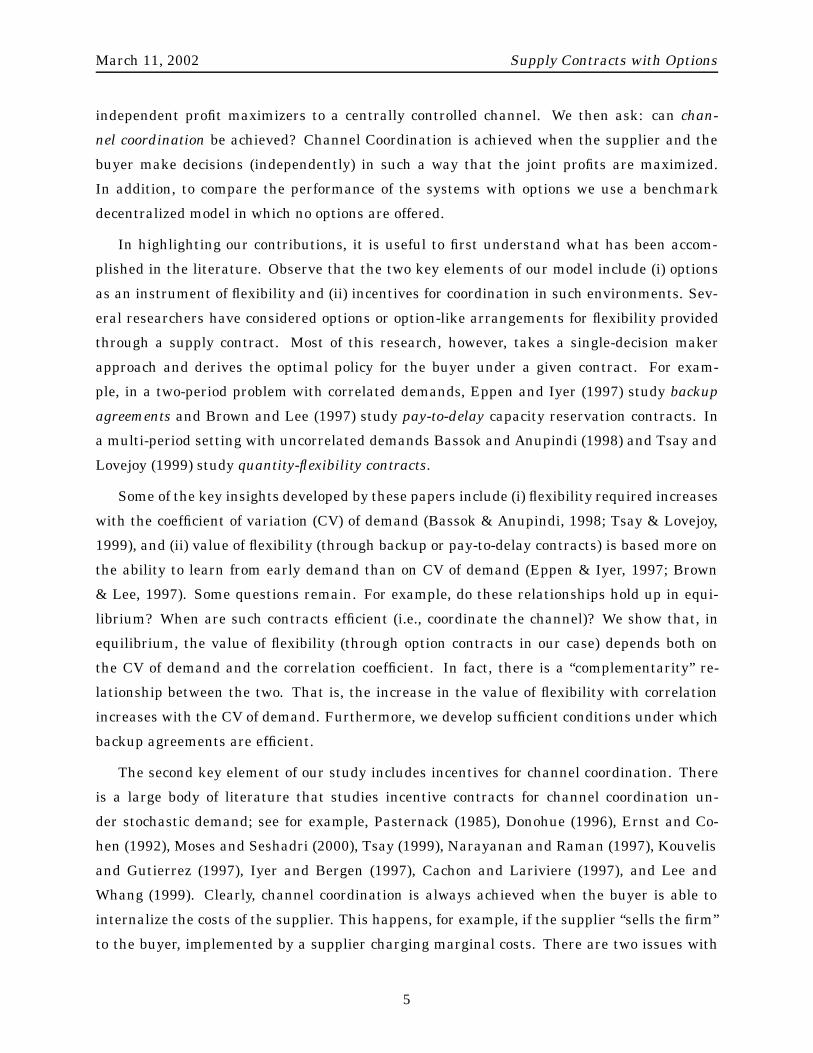
LP = Linear Prices (without Returns)B
uyer
Supp
lier
Zero Positive
Conditional Marginal Channel Risk ofAdvanced Production
Acc
ess
Adv
anta
ge t
o Sa
lvag
e M
arke
ts
RP = Linear Prices With Returns(LP; 0)
(LP; 0)(LP; 0)
(RP;�C)
(RP;�C)(RP;�C)
Figure 2: Summary of Results on Channel Coordination.
� On the other hand, we develop conditions (e.g., a.3) under which, even in the presence of
friction, coordination and arbitrary allocation of profits in the channel can be achieved.
� Furthermore, Pasternack (1985) illustrates that credit for returns (cb) can be used to
allocate the channel profits between the two parties in a single period problem; Dono-
hue (1996) illustrates the same under perfect demand correlation across periods. Propo-
sition 5 generalizes these results for a two-period problem with arbitrary correlation.
The key results are summarized in Figure 2. On the vertical axis we consider the “ac-
cess advantage to salvage markets” and on the horizontal axis we consider the “conditional
marginal channel risk of advanced production”. This results in four quadrants. In each quad-
rant, we specify a tuple. The first element of this tuple denotes the pricing scheme that
achieves channel coordination and the second denotes the profits of the supplier under the
pricing scheme. The dotted ovals suggest that the pricing scheme is only valid for a subset
of the cost region – corresponding to frictionless returns and equal salvage access – defining
the quadrant. As we can see, linear prices do not always coordinate the channel. In Barnes-
Schuster, et. al. (2002), we illustrate how non-linear prices (e.g., piecewise linear exercise
prices / quantity discount schemes) can be used to coordinate the channel regardless of the
cost parameters.
24

March 11, 2002 Supply Contracts with Options
5 Computational Study
In this section, we explore the performance of the DSNO and the DS under linear prices and
compare it to the performance of the CS. Due to the complexity of the domain being analyzed,
we are unable to completely characterize the structural properties of the solutions and hence
cannot compare the DSNO and the DS with linear prices and the CS analytically. Therefore
we resort to a numerical study. This paper has proposed two sets of actions: (i) options as an
instrument for increasing flexibility, and (ii) incentives for channel coordination. Therefore,
in the numerical study, we attempt to characterize environments, providing managerial in-
sights, under which: (i) neither action is warranted (i.e., benefits of options and incentives for
coordination are minimal), (ii) options alone are sufficient (benefits of options and coordina-
tion are large but options capture most of the benefits), and (iii) both options and incentives
for coordination useful.
We first divide the market into two broad categories: fashion goods and basic goods.14
Fashion goods are characterized (the numbers in brackets indicate the values chosen by our
numerical study) by high levels of coefficient of variation (CV) of demand (�=� 2 f0:33; 0:5g),
medium to high correlation (� 2 f0:5; 0:75; 0:9g), high margin (r = 8:0), and low salvage values
for finished goods (vsf 2 f2; 0:8g, vbf 2 f1;�0:2g) and raw material (vsr = 1:5). Basic goods, on the
other hand, are characterized by low levels of demand CV (�=� 2 f0:125; 0:25g), low correlation
(� 2 f0:0; 0:05; 0:1g), low margin (r = 5:0), and high salvage values for finished goods (vsf = 4:0,
vbf = 3:0) and raw material (vsr = 3:0). The margins are computed based on the base marginal
production cost consisting of the cost of raw material (cr = 3) and cost of labor (cL = 1). Thus
r = 8 corresponds to a maximum margin of 100% whereas r = 5:0 corresponds to a maximum
margin of 25%15. Similarly, salvage values are computed as a fraction of the base marginal
production cost of cr + cL = 4. Thus, fashion goods are characterized by low salvage values
assumed to be 20% and 50% of production cost16 and basic goods are characterized by high
salvage values assumed to be 100% of production cost. Finally, we selected penalty costs p1
and p2 from f0:25; 2:0; 19:5g to achieve low (65-68%), medium (82-87%), and high (97-98%)
levels of fill-rates for the DS.
For the purpose of our numerical study, we will assume that the supplier uses a single
wholesale price for both periods, i.e., c1 = c2. This simplifies the computations for the supplier
greatly. We believe that the nature of the results obtained will remain unaffected if we allowed14Fisher (1997) has used the classification of innovative and functional goods, respectively.15The actual retail margins are lower due to double-marginalization effect.16For the buyer it is effective salvage which is salvage less holding cost.
25

March 11, 2002 Supply Contracts with Options
for two wholesale prices. Thus the decision variables for the supplier in the DS include the
prices – (single) wholesale, option and exercise – and the production quantities. The buyer’s
decision variables are the order quantities for both periods and the number of options to
exercise in the second period. Let ��DS and ��
DSNO be the sum of the optimal profits of the
buyer and the supplier in the DS and the DSNO, respectively. In both the DS and DSNO,
the supplier optimizes her expected profit subject to a constraint that the buyer’s expected
profit be no less than his reservation profit which, without loss of generality, is assumed to be
zero. In our computational studies for both the DSNO and the DS, we observe that the prices
charged by the supplier are such that the individual rationality constraint on the buyer is
often binding. The first best solution, however, is not achieved; that is, ��DS < ��
CS .
The value of options for the channel in the DS, denoted by V O, is given by the percentage
difference between ��DS and ��
DSNO. The potential gain that could accrue from channel coor-
dination in a system that already uses options, denoted by V C, is captured by the percentage
increase from ��DS to ��
CS Finally, the joint effect of options and coordination, denoted by
V OC, is captured by the difference between the expected profits of the CS and the DSNO.
That is,
V O =��DS ���
DSNO
��DSNO
� 100 and V C =��CS ���
DS
��DS
� 100:
V OC =��CS ���
DSNO
��DSNO
� 100:
In addition, we compute the ratio V O=V OC (reported as a percentage) as a fraction of
the total possible improvement in the system (VOC) captured solely by options (VO). The
three measures along with the ratio allow us quantify the objectives of this numerical study
mentioned earlier. High values of VO suggest that options are valuable. High values of VC,
in addition, suggest that achieving coordination is important. A high V O=V OC ratio will
indicate that options capture most of the benefits whereas a low ratio will imply that we may
need to aim for coordination as well.
We perform four studies as described below. We ran a total of more than 200 scenarios
across these four studies. In the interest of space, we report a representative subset of the
results. The discussion, however, relies on the larger experimental setup. For each of these
studies, we attempt to give an explanation for the behavior of V O, V C, and V OC based on
a set of operational actions. It is hard, however, to similarly explain the change in the ratio
V O=V OC (why it increases or decreases), since monotonicity of V O and V OC do not guarantee
a certain directional change in their ratio.
26

March 11, 2002 Supply Contracts with Options
Before we discuss the various studies in detail, we discuss a hypothesis that correlates
the metric VC with the quantities purchased in the DS and the CS. This, coupled with the
pricing power of the supplier as a Stackelberg leader, will be useful in explaining the behavior
of VC in several of the scenarios later. Let QDS and QCS be the total quantity of raw material
purchased in DS and CS respectively. Our hypothesis is that the ratio QDS=QCS is a good
proxy for the metric VC. That is, as QDS=QCS increases VC decreases. The basic intuition
is that double-marginalization reduces the quantity purchased in the DS leading to lower
profits. If QDS is closer to QCS, then the double-marginalization effect is lower and the need
for coordination will also be lower leading to a lower VC. This is certainly true for a single
period newsvendor problem. In applying this argument to our model, we are ignoring the
effect of allocation of quantities across the two periods. We observe that the effect of total
quantities usually dominates the allocation effect. Furthermore, based on classical single-
period newsvendor analysis, we will use a critical fractile as a measure of the quantities.
Specifically, for the DS it is �DS = r+p�cr+p+h�v and for the CS it is �CS = r+p�(cr+cL)
r+p+h�v , where r
represents the unit revenue, p is the unit penalty cost, c is the unit wholesale price in DS,
h represents the holding cost, v represents the salvage value, and (cr + cL) represents the
production cost. While the quantities in our model are not so neatly captured by a critical
fractile, nevertheless they serve as useful approximations. These critical fractiles will be
useful in comparative statics to explain the behaviors of QDS and QCS and hence that of
VC. Our explanations are based on conjectures formed from the extensive numerical studies.
Formal verification of these conjectures are potential areas for future research.
5.1 Effect of Demand Risk
Here we evaluate the value of options and coordination for both types of goods with changes
in demand CV and correlation under equal access to salvage markets. The results are sum-
marized in Table 2. We assume the following values for other parameters: = 0:5, hs = 0:4
and p1 = p2 = 2:0.
� Effect of Demand Variability
In Table 2, the results for demand CV appear in adjacent sets of columns. Comparing the
metrics across these columns, we observe that VO and VOC increase with demand CV. In
general increasing CV of demand increases the probability of mismatch between supply and
demand in both periods. The use of options, however, allows the buyer to compensate for this
mismatch using exercised options in two ways: (a) excess inventory / demand at the end of the
first period is corrected, and (b) the potential second period mismatch is minimized by demand
27

March 11, 2002 Supply Contracts with Options
updating. We therefore observe that VO increases with demand CV. A similar phenomenon in
the CS explains the behavior of VOC.
Next, we observe from Table 2 that VC increases with CV of demand. That is, coordination
is more valuable when demand variability is higher. Recall our discussion on QDS , QCS and
VC. For a given a wholesale price in the DS, �DS < �CS . This implies that QDS increases at a
rate slower than QCS and hence the ratio QDS=QCS is decreasing with CV of demand for fixed
prices. Consequently coordination will be more valuable with increasing demand CV for fixed
prices. The buyer’s profit, however, reduces with CV of demand. To incent the buyer to buy
more products, the supplier decreases the wholesale and option prices. The decreasing prices
reduce double marginalization increasing the ratio QDS=QCS . Thus, CV of demand decreases
the ratio whereas the supplier’s pricing power increases it. How do these opposing forces play
out? Whenever the critical fractiles in DS and CS are such that �DS << �CS (e.g., low-medium
penalty costs or low salvage values), changes in CV of demand dominate the supplier’s pricing
power effect. Consequently, we observe that the ratio QDS=QCS is decreasing with CV leading
to an increasing VC as in Table 2(a). When both the critical fractiles are high and close to
each other (e.g., due to high penalty costs), we observe (results not reported here) that often
the supplier’s wholesale pricing power reverses the direction of change in the ratio QDS=QCS ,
and VC decreases with CV. To summarize, for fashion goods VC increases with CV of demand
for low to moderate service levels, whereas it decreases with CV of demand for high service
levels. For basic goods, since the value of options are low, the supplier’s pricing power (which
affects both the wholesale and option prices) is dominated by the effect of CV of demand at
fixed prices. Consequently (see Table 2(b)), we observe that VC increases with CV of demand.
� Effect of Demand Correlation
Higher correlation implies that the first period demand realization is more informative
about the second period demand. Options allow the channel to exploit this information by
shifting procurement from (inflexible) commitments to (flexible) options. Thus VO and VOC
increase with demand correlation.
Demand correlation impacts operational decisions in two ways. In the first period before
any decisions are made, total demand variability across the two periods increases with corre-
lation. This affects the committed quantities. After the first period, the second period demand
variability decreases with correlation. Based on the earlier discussion on the effect of demand
variability on VC, we then conclude that there are two opposing forces acting on VC due to
correlation. In the beginning, VC increases as total demand variability across the two periods
increases with correlation whereas for the second period VC decreases as the remaining de-
28

March
11,2002S
upplyC
ontractsw
ithO
ptions
Demand Demand CV = 0.33 Demand CV = 0.5
Correlation �DSNO QDS=QCS VO VOC VO/VOC VC �DSNO QDS=QCS VO VOC VO/VOC VC
Medium Salvage (vsf = 2:0, vbf = 1:0)
0.5 1150.40 82.61% 1.81 13.19 13.71 11.18 895.03 80.95% 2.43 15.09 16.10 12.36
0.75 1126.29 85.60% 6.57 16.51 39.81 9.32 864.59 83.91% 9.24 20.89 44.24 10.66
0.9 1112.50 89.30% 13.15 20.95 62.79 6.89 846.60 90.08% 19.32 29.24 66.07 8.31
Low Salvage (vsf = 0:8, vbf = �0:2)
0.5 1078.64 84.39% 3.00 13.25 22.61 9.96 785.05 83.61% 4.55 15.79 28.79 10.76
0.75 1051.15 88.32% 9.61 18.78 51.14 8.37 747.90 86.89% 15.89 26.88 59.13 9.48
0.9 1035.40 89.89% 18.46 25.79 71.59 6.18 726.52 91.70% 31.57 41.35 76.36 7.43
Table 2(a): Demand and Salvage Risk for Fashion GoodsDemand Demand CV = 0.125 Demand CV = 0.25
Correlation �DSNO QDS=QCS VO VOC VO/VOC VC �DSNO QDS=QCS VO VOC VO/VOC VC
0 249.39 89.51% 0.06 1.94 3.32 1.88 162.61 83.12% 0.16 3.59 4.55 3.42
0.05 248.49 88.13% 0.21 2.21 9.71 2.00 160.85 80.86% 0.61 4.43 13.80 3.80
0.1 247.60 86.80% 0.44 2.56 17.08 2.11 159.12 78.66% 1.29 5.50 23.46 4.16
Table 2(b): Demand Risk for Basic Goods
Fashion Goods Basic Goods
Penalty Cost �DSNO �DS VO VOC VO/VOC VC �DSNO �DS VO VOC VO/VOC VC
low 822.93 870.89 5.83 42.08 13.85 34.26 218.42 218.45 0.02 9.94 0.16 9.92
medium 864.59 944.49 9.24 20.89 44.24 10.66 162.61 162.87 0.16 3.59 4.55 3.42
high 432.15 602.11 39.33 42.31 92.96 2.14 23.17 26.48 14.26 28.81 49.51 12.73
Table 3: Serviceability for Fashion and Basic Goods.
29

March 11, 2002 Supply Contracts with Options
mand variability decreases. The overall effect on VC with respect to correlation will depend
on which of these effects dominate. For fashion goods, options partially mitigate the first ef-
fect such that VC is decreasing with correlation. For basic goods, however, there is little value
of options and VC increases with correlation.
Finally, we also observe (Table 2(a)) that the increase in both VO and VOC with correla-
tion, increases with the CV of demand. This is a complementarity result implying that more
information is more valuable when demand variability is higher, provided we have a mecha-
nism to respond to it.
5.2 Effect of Salvage Risk
We say that salvage risk is high when salvage value is low and vice versa. Comparing the
sets of results for the two levels of salvage values in Table 2(a), we observe that both VO and
VOC increase as salvage value decreases. Intuitively, when salvage value decreases, both the
supplier and the buyer, respectively, under-produce or under-order to avoid the risk of salvage.
Flexibility provided through options allows the players to mitigate this risk and increase the
channel profits.
There are two forces that impact VC. First, in the absence of any pricing effects and using
the analogy from a single period model, we expect that VC will increase with salvage value.
This is due to the fact that an increase in salvage value impacts �CS more than �DS . This
implies that QCS will increase at a rate faster that QDS , decreasing the ratio QDS=QCS , and
increasing VC. The second effect, viz., the pricing power that the supplier exercises in the
channel, works as follows. As profits of the buyer increase with salvage value, the supplier
attempts to extract away some of these higher profits by increasing the prices. This, how-
ever, increases the double marginalization effect increasing VC further. Thus the two effects
reinforce each other and we observe that VC increases in salvage value.
5.3 Effect of Serviceability
We test the effect of serviceability (measured as fill-rate) for both types of goods by varying
the penalty costs. Observe that service levels are proportional to penalty costs. The results
are shown in Table 3. The values of other parameters for fashion goods are hs = 0:4, CV = 0:5,
= 0:5, vsf = 2, vbf = 1, and � = 0:75; similarly the values of other parameters for basic goods
are hs = 0:4, CV = 0:25, = :5, vsf = 4, vbf = 3, and � = 0. We make the following observations.
30
March 11, 2002 Supply Contracts with Options
We observe that VO increases with serviceability. As penalty costs increase, the need to
more accurately match supply and demand increases. The buyer, with proper incentives from
the supplier, achieves this by buying more options and postponing more of his orders from
commitments to exercised options which increases VO.
Next we observe that both VOC and VC are convex – decreasing and eventually increasing
– in penalty costs. Our hypothesis is based on the following three effects that impact profits
in both decentralized systems17 – DSNO and DS:
� Under the first effect, when (wholesale / option) prices are unchanged, the buyer’s profit
decreases and the supplier’s profit increases with penalty cost. The total system profits
in DSNO / DS may then decrease or increase with penalty costs.
� The second effect, viz., the pricing power that the supplier exercises in the channel,
works as follows. In general, as penalty cost increases, the buyer tends to buy more
goods to satisfy a higher service level. A higher penalty cost, on the other hand, allows
the supplier to increase prices without significantly affecting the service level. The in-
creasing prices lead to a larger double marginalization effect decreasing profits in DSNO
and DS. This happens until the buyer’s individual rationality constraint18 (IRC) is bind-
ing.
� The last effect is also related to the pricing power of the supplier but when the IRC is
binding. As penalty cost increases and the supplier increases the wholesale price (second
effect), the buyer’s profit will ultimately turn negative. To satisfy the IRC, however, the
supplier then has to decrease the wholesale price. This decreases the double marginal-
ization effect putting upward pressure on profits in DSNO and DS.
Regardless of whether the first effect leads to an increase or decrease in system profits, in
combination with the second effect, we observe that the total system profits always decrease
with penalty costs. When the IRC kicks in, the behavior of profits depend on a combination of
the first and third effect. In this region we observe that initially the third effect dominates,
increasing profits. Ultimately, the first effect dominates and profits start decreasing again.
Thus, we expect the profits in DSNO and DS to exhibit a convex-concave behavior. This is
indeed our observation in our larger numerical study. In Table 3 for fashion goods, the IRC is
not binding for low penalty but subsequently is, giving rise to a concave behavior. In the same17We find it easier to explain VC based on the behavior of profits rather than quantities as before.18He needs to make at least non-zero profit.
31

March 11, 2002 Supply Contracts with Options
table for basic goods the IRC is always binding. Consequently, we see the decreasing part of
the profit curve as the first effect dominates the third.
Observe that profits in CS always decrease with penalty costs. For fashion goods profits
in the DSNO and DS are concave in the region and we see that VOC and VC are convex. For
basic goods, profits in DSNO and DS are decreasing in the region (the IRC is always binding).
Initially (when penalty cost is low), however, the rate of decrease in profits of DSNO and DS
is less than that of CS due to the third effect identified above. This leads to decreasing VOC
and VC. Ultimately, the first effect dominates and profits in DSNO and DS decline faster than
in the CS leading to an increasing VOC and VC. The net result is that even for basic goods
VOC and VC are convex.
5.4 Effect of Supplier Flexibility
To study the effect of flexibility available to a supplier on the value of options and coordina-
tion for fashion goods, we varied the incremental cost of expedited production. The results
are presented in Table 4. The values of other parameters are hs = 0:4, CV = 0:5, vsf = 2,
vbf = 1, � = 0:75, p1 = p2 = 19:5. We make the general observation that both VO and VOC
Profits Total Number of Advanced in Committed of Options Production QDS=QCS VO VOC VO/VOC VC
DSNO Qty. (X2) M
2.0 432.15 183 590 590 95.63% 18.11 21.06 85.99 2.501.5 432.15 183 604 540 96.40% 19.08 23.41 81.52 3.631.0 432.15 183 612 454 96.40% 24.37 28.57 85.30 3.380.5 432.15 183 622 239 96.59% 39.33 42.31 92.96 2.140.4 432.15 183 634 0 97.80% 46.57 49.28 94.51 1.85
Table 4: Effect of Supplier Flexibility
increase with supplier flexibility (decreasing ). In the DS, as the supplier’s cost of expedited
production decreases, she reduces the option price (values not shown here), thus incentivizing
the buyer to buy more options. The buyer buys more options (as seen from the column labeled
M of the table) and the supplier produces less in advance (see the column labeled ‘advanced
production’) improving the match between supply and demand. This increases VO. The same
effects are present in the CS and hence VOC too increases.
We observe that VC is concave – increases and then decreases – with flexibility. Once
again there are two effects to consider. First, when prices are kept unchanged, we expect the
32
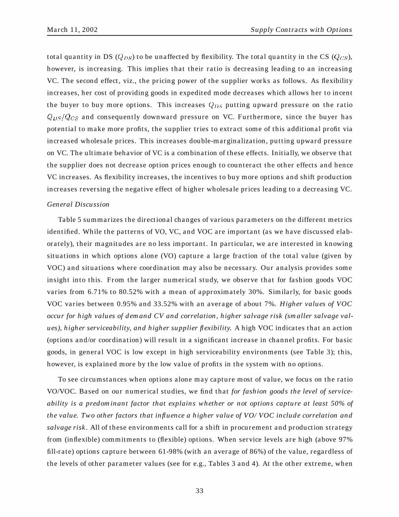
March 11, 2002 Supply Contracts with Options
total quantity in DS (QDS) to be unaffected by flexibility. The total quantity in the CS (QCS),
however, is increasing. This implies that their ratio is decreasing leading to an increasing
VC. The second effect, viz., the pricing power of the supplier works as follows. As flexibility
increases, her cost of providing goods in expedited mode decreases which allows her to incent
the buyer to buy more options. This increases QDS putting upward pressure on the ratio
QDS=QCS and consequently downward pressure on VC. Furthermore, since the buyer has
potential to make more profits, the supplier tries to extract some of this additional profit via
increased wholesale prices. This increases double-marginalization, putting upward pressure
on VC. The ultimate behavior of VC is a combination of these effects. Initially, we observe that
the supplier does not decrease option prices enough to counteract the other effects and hence
VC increases. As flexibility increases, the incentives to buy more options and shift production
increases reversing the negative effect of higher wholesale prices leading to a decreasing VC.
General Discussion
Table 5 summarizes the directional changes of various parameters on the different metrics
identified. While the patterns of VO, VC, and VOC are important (as we have discussed elab-
orately), their magnitudes are no less important. In particular, we are interested in knowing
situations in which options alone (VO) capture a large fraction of the total value (given by
VOC) and situations where coordination may also be necessary. Our analysis provides some
insight into this. From the larger numerical study, we observe that for fashion goods VOC
varies from 6.71% to 80.52% with a mean of approximately 30%. Similarly, for basic goods
VOC varies between 0.95% and 33.52% with an average of about 7%. Higher values of VOC
occur for high values of demand CV and correlation, higher salvage risk (smaller salvage val-
ues), higher serviceability, and higher supplier flexibility. A high VOC indicates that an action
(options and/or coordination) will result in a significant increase in channel profits. For basic
goods, in general VOC is low except in high serviceability environments (see Table 3); this,
however, is explained more by the low value of profits in the system with no options.
To see circumstances when options alone may capture most of value, we focus on the ratio
VO/VOC. Based on our numerical studies, we find that for fashion goods the level of service-
ability is a predominant factor that explains whether or not options capture at least 50% of
the value. Two other factors that influence a higher value of VO/VOC include correlation and
salvage risk. All of these environments call for a shift in procurement and production strategy
from (inflexible) commitments to (flexible) options. When service levels are high (above 97%
fill-rate) options capture between 61-98% (with an average of 86%) of the value, regardless of
the levels of other parameter values (see for e.g., Tables 3 and 4). At the other extreme, when
33
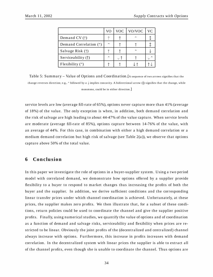
March 11, 2002 Supply Contracts with Options
VO VOC VO/VOC VC
Demand CV (") " " " l
Demand Correlation (") " " " l
Salvage Risk (") " " " #
Serviceability (") " # " " # "
Flexibility (") " " # " " #
Table 5: Summary – Value of Options and Coordination.[A sequence of two arrows signifies that the
change reverses direction; e.g., " followed by a # implies concavity. A bidirectional arrow (l) signifies that the change, while
monotone, could be in either direction.]
service levels are low (average fill-rate of 65%), options never capture more than 41% (average
of 18%) of the value. The only exception is when, in addition, both demand correlation and
the risk of salvage are high leading to about 44-47% of the value capture. When service levels
are moderate (average fill-rate of 85%), options capture between 14-76% of the value, with
an average of 44%. For this case, in combination with either a high demand correlation or a
medium demand correlation but high risk of salvage (see Table 2(a)), we observe that options
capture above 50% of the total value.
6 Conclusion
In this paper we investigate the role of options in a buyer-supplier system. Using a two period
model with correlated demand, we demonstrate how options offered by a supplier provide
flexibility to a buyer to respond to market changes thus increasing the profits of both the
buyer and the supplier. In addition, we derive sufficient conditions and the corresponding
linear transfer prices under which channel coordination is achieved. Unfortunately, at these
prices, the supplier makes zero profits. We then illustrate that, for a subset of these condi-
tions, return policies could be used to coordinate the channel and give the supplier positive
profits. Finally, using numerical studies, we quantify the value of options and of coordination
as a function of demand and salvage risks, serviceability and flexibility when prices are re-
stricted to be linear. Obviously the joint profits of the (decentralized and centralized) channel
always increase with options. Furthermore, this increase in profits increases with demand
correlation. In the decentralized system with linear prices the supplier is able to extract all
of the channel profits, even though she is unable to coordinate the channel. Thus options are
34

March 11, 2002 Supply Contracts with Options
useful instruments to increase flexibility and channel profits. The risk to supplier of offering
a higher level of flexibility is partly mitigated by the use of options. Thus options can be an
effective mechanism to implement in-season replenishments in the channel.
We have also illustrated how return policies, in conjunction with linear prices, can be used
to coordinate the channel and allow the supplier to extract the channel profits. These results
significantly expand the scope of return policies beyond those studied in the context of “single”
period models by Pasternack (1985) and Donohue (1996).
Our model assumes that the length of the first period is exogenous. A buyer updates de-
mand at the end of the first period and exercises options. One could argue that the timing of
the demand update should be a decision variable for the buyer. Ideally, a buyer may update
the demand density in a dynamic fashion after observing a certain level of sales. An alternate
approach could be that the timing of demand update is announced a priori (at the beginning
of the horizon) so that the supplier could make some appropriate planning decisions. A buyer
then decides on this optimal timing, in addition to the various order quantities. In a prelim-
inary study, we use a discrete time model to study the sensitivity of the timing of updates to
the level of correlation, labor costs, etc. Numerical testing shows that the optimal timing of
demand updates is usually later in the DS (with linear prices) than in the CS. A complete
analysis of this issue is an area of further research.
Finally, we have assumed information symmetry between the buyer and the supplier.Analysis under information asymmetry (regarding costs and/or demand parameters) are alsoareas of future research.
References
BARNES-SCHUSTER, D., Y. BASSOK, AND R. ANUPINDI (2002). Supply Contracts with Options: Flex-
ibility, Information, and Coordination. Working Paper; Stern School of Business, New York Uni-
versity, New York, NY 10012. First version Feb. 1998; Last Revised March 2002.
BASSOK, Y. AND R. ANUPINDI (1998). Analysis of Supply Contracts with Commitments and Flexibil-
ity. March 1995. Revised August 1998. Northwestern University, Evanston, IL 60208.
BASSOK, Y., R. SRINIVASAN, A. BIXBY, AND H. WIESEL (1997). Design of Component Supply Con-
tracts with Commitment Revision Flexibility. IBM Journal of Research and Development, 41(6).
BROWN, A. O. AND HAU L. LEE (1997). Optimal Pay–to–Delay Capacity Reservation with Applica-
tion to the Semiconductor Industry. Working Paper. Department of Industrial Engineering and
Engineering Management, Stanford University, Stanford, CA.
35
March 11, 2002 Supply Contracts with Options
CACHON, G. AND MARTIN LARIEVIERE (1997). Contracting to Assure Supply or What Did the Supplier
Know and When Did He Know It? The Fuqua School of Business, Duke University, Durham, NC.
CHANG, C. (1996). Semiconductor Contract Manufacturing. Report #SCMS–WW–FR–9601, Dataquest
Corporation.
DONOHUE, K. (1996). Supply Contracts and Fashion Goods: Optimizing Channel Profit. The Wharton
School, University of Pennsylvania, Philadelphia, PA.
EPPEN, G. AND ANANTH IYER (1997). Backup Agreements in Fashion Buying – The Value of Upstream
Flexibility. Management Science, 43(11), 1469–1484.
ERNST, R. AND MORRIS COHEN (1992). Analysis of Coordinated Alternatives in an Manufac-
turer/Dealer Inventory System under Stochastic Demand. Production and Operations Manage-
ment Journal, 1(3), 254–268.
FARLOW, D., G. SCHMIDT, AND A. TSAY (1995). Supplier Management at Sun Microsystems. Case
Study, Graduate School of Business, Stanford University, Stanford, CA.
FEDERGRUEN, A. AND P. ZIPKIN (1986). An Inventory Model with Limited Production Capacity and
Uncertain Demands II: Discounted Cost Criterion. Mathematics of Operations Research, 11(2),
208–215.
FISHER, M. AND A. RAMAN (1996). Reducing the Cost of Demand Uncertainty Through Accurate
Response to Early Sales. Operations Research, 44(1), 87–89.
FISHER, M. L. (1997). What is the Right Supply Chain for your Product? Harvard Business Review,
March-April, 105–116.
FISHER, M. L., JANINE H. HAMMOND, WALTER R. OBERMEYER, AND ANANTH RAMAN (1994). Mak-
ing Supply and Demand Meet in an Uncertain World. Harvard Business Review, 83–93.
FRAZIER, R. (1986). QR Inventory Replenishment. In Proceedings of the 75th NRMA Conference.
HAMMOND, J. H. (1990). Quick Response in The Apparel Industry. The Harvard Business School,
Note #9-60-038.
HAMMOND, J. H. (1992). Coordination as the Basis for Quick Response: A Case of “Virtual” Integration
in Supply Networks. The Harvard Business School, Working paper #92-007.
HUNTER, N., R.E. KING, AND H.L.W. NUTTLE (1996). Evaluation of Traditional and Quick Response
Retailing Procedures using Stochastic Simulation Model. Journal of the Textile Institute, 87(1,
part 2), 42–55.
IYER, A. AND MARK BERGEN (1997). Quick Response in Manufacturer Retailer Channels. Manage-
ment Science, 43(4).
KING, R. AND N.A. HUNTER (1996). The Impact of Size Distribution Forecast Errors on Retail Per-
formance. NCSU-IE Technical Report # 95-8, Industrial Engineering Department, N.C. State
University, Raleigh, NC.
36

March 11, 2002 Supply Contracts with Options
KOUVELIS, P. AND G. GUTIERREZ (1997). The Newsvendor Problem in a Global Market: Optimal
Centralized and Decentralized Control Policies for a Two-Market Stochastic Inventory Systems.
Management Science, 43(5), 571–585.
KRAVETZ, S. (1999). Mattel Revamps Retail Strategy To Boost Sales, Find New Avenues. Wall Street
Journal. February 18.
LEE, H. L. AND SEUNJIN WHANG (1999). Decentralized Multi-Echelon Supply Chains: Incentives
and Information. Management Science, 45(5), 633–640.
LOVEJOY, J. (1999). Personal Communication.
MOSES, M. AND SRIDHAR SESHADRI (2000). Policy Mechanisms for Supply Chain Coordination. IIE
Transactions in Operations Engineering, 32(3), 245–262.
NARAYANAN, V. AND ANANTH RAMAN (1997). Contracting for Inventory in a Distribution Channel
with Stochastic Demand and Substitute Products. Working paper; Harvard Business School.
NUTTLE, H., N.A. HUNTER, AND R.E. KING (1991). A Stochastic Model of the Apparel Retailing
Process for Seasonal Apparel. Journal of the Textile Institute, 82(2), 247–259.
PADMANABHAN, V. AND I.P.L. PNG (1995). Return Policies: Make Money by Making Good. Sloan
Management Review, Fall, 65–72.
PASTERNACK, B. A. (1985). Optimal Pricing and Return Policies for Perishable Commodities. Market-
ing Science, 4(2), 166–176.
PINNOW, A. AND R.E. KING (1997). Break-even Cost for Traditional Versus Quick Response Apparel
Suppliers. NCSU-IE Technical Report # 97-4, Industrial Engineering Department, N.C. State
University, Raleigh, NC.
TIROLE, J. (1990). The Theory of Industrial Organization. The MIT Press, Cambridge, Massachusetts.
TSAY, A. (1999). The Quantity Flexibility Contract and Supplier-Customer Incentives. Management
Science, 45(10).
TSAY, A. AND WILLIAM LOVEJOY (1999). Quantity Flexibility Contracts and Supply Chain Perfor-
mance. Journal of Manufacturing and Service Operations Management, 1(2).
WHALEN, C. (1993). Quick Response in Action-and Beyond. Bobin.
37

March 11, 2002 Supply Contracts with Options
A Expressions for the Profit Functions
� Profit function of the buyer in DS:
�bDS(X1; X2; X3) = J1(X1) + J2(X2) + J3(X3);
where,
J1(X1) = �p2�2 � �1(p1 + p2)� (p1 + hb1)
Z X1
0
(X1 � d1)dFD1(d1) + (p1 + c2 � c1)X1
J2(X2) = (p2 + r � (c2 � co))X2 + (p2 + r � ce)
Z 1
X2�Æd
�
(Æd + �d1 �X2)dFD1(d1)
�(p2 + r � vbf )
Z X2�Æd
�
0
Z X2�d1
0
(X2 � d1 � d2)dFD2jd1(d2)dFD1(d1)
�(p2 + r � vbf )
Z 1
X2�Æd
�
Z Æd+(��1)d1
0
(Æd + (� � 1)d1 � d2)dFD2jd1(d2)dFD1(d1) (9)
J3(X3) = �coX3 � (p2 + r � ce)
Z 1
X3�Æd
�
(Æd + �d1 �X3)dFD1(d1)
+(p2 + r � vbf )
"Z 1
X3�Æd
�
Z Æd+(��1)d1
0
(Æd + (� � 1)d1 � d2)dFD2jd1(d2)dFD1(d1)
�
Z 1
X3�Æd
�
Z X3�d1
0
(X3 � d1 � d2)dFD2 jd1(d2)dFD1(d1)
#(10)
� Profit function of the system in CS, vsf � vbf and vsr + cL(1 + ) > vbf :
�CS(Xc1 ; X
cL; X
c3) = Jc1(X
c1) + JcL(X
cL) + Jc3(X
c3);
where
Jc1(Xc1) = �p2�2 � �1(p1 + p2)� (p1 + hb1)
Z Xc1
0
(Xc1 � d1)dFD1
(d1) + (p1 + hs)Xc1 (11)
JcL(XcL) = (p2 + r � vsr � cL � hs)Xc
L
+(p2 + r � vsr � cL(1 + ))
Z 1
XcL�Æc
2�
(Æc2 + �d1 �XcL)dFD1
(d1)
�(p2 + r � vbf )
24Z Xc
L�Æc
2�
0
Z XcL�d1
0
(XcL � d1 � d2)dFD2jd1(d2)dFD1
(d1)
+
Z 1
XcL�Æc
2�
Z Æc2+(��1)d1
0
(Æc2 + (� � 1)d1 � d2)dFD2 jd1(d2)dFD1(d1)
#(12)
Jc3(Xc3) = �(cr � vsr)X
c3 � (p2 + r � vsr � cL(1 + ))
Z 1
Xc3�Æc
2�
(Æc2 + �d1 �Xc3)dFD1
(d1)
+(p2 + r � vbf )
"Z 1
Xc3�Æc
2�
Z Æc2+(��1)d1
0
(Æc2 + (� � 1)d1 � d2)dFD2jd1(d2)dFD1(d1)
�
Z 1
Xc3�Æc
2�
Z Xc3�d1
0
(Xc3 � d1 � d2)dFD2jd1(d2)dFD1
(d1)
#: (13)
38

March 11, 2002 Addendum to Supply Contracts with Options
Addendum toCoordination and Flexibility in Supply Contracts with Options
B Notation
ci unit wholesale price for firm orders to be delivered in period i.
ce unit exercise price.
co unit option price.
cL unit labor cost of production.
cr unit cost of raw material.
additional unit labor cost of production in the expedited mode.
XL production quantity of the supplier in the cheaper mode of production;
that is at labor cost of cL per unit.
vsr unit salvage value of raw material for the supplier.
vsf unit salvage value of finished goods for the supplier.
hs unit period one holding cost for finished goods at the supplier.
Qi order quantity to be delivered at the beginning of
period i, i 2 f1; 2g at a wholesale price of ci.
M number of options purchased at the beginning of
period one at a unit price of co.
m number of options exercised at the beginning of period two at a price of c e.
r unit selling price of finished good to the consumer.
hbi unit holding cost of the buyer in period i 2 f1; 2g.
pi unit shortage penalty cost incurred by the buyer in period i 2 f1; 2g.
~vbf unit salvage value of finished goods for the buyer.
vbf effective salvage value of finished goods for the buyer; equal to ~v bf � hb2.
Di demand in period i 2 f1; 2g assumed to be normally distributed.
�i mean of Di.
�i standard deviation of Di.
� correlation coefficient of D1 and D2.
FDi(�) conditional distribution function of Di.
fDi(�) conditional density function of Di.
�(�) distribution function of standard normal.
cb price the supplier gives the buyer for goods returned at the end of the season.
tbs cost the supplier pays to ship goods back from the buyer at the end of the season.
i

March 11, 2002 Addendum to Supply Contracts with Options
C Expressions for the Remaining Profit Functions
� Profit function of the system in CS, vsf � vbf and vsr + cL(1 + ) � vbf :
�CS(Xc1 ; X
cL; X
c3) = Jc1(X
c1) + JcL(X
cL) + Jc3(X
c3);
where XcL = Xc
3 , Jc1(Xc1) is as in (11) and
Jc3(Xc3) = (p2 + r � cr � cL � hs)Xc
3 � (p2 + r � vbf )
Z Xc3
0
(Xc3 � d12)dFD1+D2
(d12) (14)
� Profit function of the system in CS, vsf > vbf and vsr + cL(1 + ) � vsf :
�CS(Xc1 ; X
cL; X
c3) = Jc1(X
c1) + Jc3(X
c3);
where XcL = Xc
3 and
Jc1(Xc1) = �p2�2 � �1(p1 + p2)� (p1 + hb1)
Z Xc1
0
(Xc1 � d1)dFD1
(d1)
+(p1 + p2 + r � vsf + hs)Xc1 +
�p2 + r � vsf
� Z 1
Xc1�Æc
1�
(Æc1 + �d1 �Xc1)dFD1
(d1)
�(p2 + r � vbf )
24Z Xc
1�Æc
1�
0
Z Xc1�d1
0
(Xc1 � d1 � d2)dFD2jd1(d2)dFD1
(d1)
+
Z 1
Xc1�Æc
1�
Z Æc1+(��1)d1
0
(Æc1 + (� � 1)d1 � d2)dFD2jd1(d2)dFD1(d1)
#; (15)
Jc3(Xc3) = (vsf � cr � cL � hs)Xc
3 � (p2 + r � vsf )
Z 1
Xc3�Æc
1�
(Æc1 + �d1 �Xc3)dFD1
(d1)
�(p2 + r � vbf )
"Z 1
Xc3�Æc
1�
Z Xc3�d1
0
(Xc3 � d1 � d2)dFD2jd1(d2)dFD1
(d1)
�
Z 1
Xc3�Æc
1�
Z Æc1+(��1)d1
0
(Æc1 + (� � 1)d1 � d2)dFD2jd1(d2)dFD1(d1)
#: (16)
� Profit function of the system in CS, vsf > vbf and vsr + cL(1 + ) > vsf :
�CS(Xc1 ; X
cL; X
c3) = Jc1(X
c1) + JcL(X
cL) + Jc3(X
c3);
where J c1(Xc1) is as in (15), Jc3(X
c3) is as in (13), and
JcL(XcL) = (vsf � vsr � cL � hs)Xc
L � (p2 + r � vsf )
Z 1
XcL�Æc
1�
(Æc1 + �d1 �XcL)dFD1
(d1)
+ (p2 + r � cL(1 + )� vsr)
Z 1
XcL�Æc
2�
(Æc2 + �d1 �XcL)dFD1
(d1)
�(p2 + r � vbf )
24Z Xc
L�Æc
2�
XcL�Æc
1�
Z XcL�d1
0
(XcL � d1 � d2)dFD2jd1(d2)dFD1
(d1)
ii

March 11, 2002 Addendum to Supply Contracts with Options
�
Z 1
XcL�Æc
1�
Z Æc1+(��1)d1
0
(Æc1 + (� � 1)d1 � d2)dFD2jd1(d2)dFD1(d1)
+
Z 1
XcL�Æc
2�
Z Æc2+(��1)d1
0
(Æc2 + (� � 1)d1 � d2)dFD2jd1(d2)dFD1(d1)
#: (17)
D Proofs
Derivation of (7)
Let us begin by simplifying (6). Collecting terms and taking expectations gives
�b1(Q1; Q2;M) = ED1
�rD1 � r(D1 �Q1)
+ � coM � c1Q1 � c2Q2 � hb1(Q1 � d1)+ � p1(d1 �Q1)
+
+ED2[�b
2(m�jd1)]
�= �coM � c1Q1 � c2Q2 � (hb1 + p1)
Z Q1
0
(Q1 � d1)dFD1(d1)� p1(�1 �Q1)
+ED1[�b
2(m�jd1) + rD1 � r(D1 �Q1)
+]: (18)
Expanding out ED1[�b
2(m�jd1) + rD1 � r(D1 �Q1)
+], we get
ED1[�b
2(m�jd1) + rD1 � r(D1 �Q1)
+]
=
Z 1
0
�(r � ce)m
� � p2 (�2 � (� � 1)�1 + �D1 �Q1 �Q2 �m�) + r(Q1 +Q2)
�(p2 + r � vbf )
Z Q1+Q2�d1+m�
0
(Q1 +Q2 +m� � d1 � d2)dFD2jd1(d2)
�dFD1
(d1)
= (p2 + r � ce)
Z 1
0
m�dFD1(d1)� p2 (�1 + �2 �Q1 �Q2) + r(Q1 +Q2)
�(p2 + r � vbf )
0@Z Q1+Q2�Æ
d
�
0
Z Q1+Q2�d1
0
(Q1 +Q2 � d1 � d2)dFD2jd1(d2)dFD1(d1)
+
Z Q1+Q2+M�Æd
�
Q1+Q2�Æd
�
Z Æd+(��1)d1
0
(Æd + (� � 1)d1 � d2)dFD2jd1(d2)dFD1(d1)
+
Z 1
Q1+Q2+M�Æd
�
Z Q1+Q2+M�d1
0
(Q1 +Q2 +M � d1 � d2)dFD2jd1(d2)dFD1(d1)
!: (19)
Substituting, (X1; X2; X3) = (Q1; Q1 +Q2; Q1 +Q2 +M), we rewrite �b(Q1; Q2;M) as
�bDS(X1; X2; X3) = �coX3 + (r � (c2 � co))X2 � (c2 � c1)X1 � (hb1 + p1)
Z X1
0
(X1 � d1)dFD1(d1)
�p1(�1 �X1) +ED1[�b
2
�(Æd + �D1 �X2)
+ � (Æd + �D1 �X3)+�]
+rED1
�(Æd + �D1 �X2)
+ � (Æd + �D1 �X3)+ � (X2 +m� �D1)
+�: (20)
where
ED1[�b
2((Æd + �D1 �X2)
+ � (Æd + �D1 �X3)+) + rm� � r(X2 +m� �D1)
+]
iii

March 11, 2002 Addendum to Supply Contracts with Options
= �p2 (�1 + �2 �X2) + (p2 + r � ce)
Z 1
X2�Æd
�
(Æd + �d1 �X2)dFD1(d1)
� (p2 + r � ce)
Z 1
X3�Æd
�
(Æd + �d1 �X3)dFD1(d1)
�(p2 + r � vbf )
Z X2�Æd
�
0
Z X2�d1
0
(X2 � d1 � d2)dFD2 jd1(d2)dFD1(d1)
�(p2 + r � vbf )
Z X3�Æd
�
X2�Æd
�
Z Æd+(��1)d1
0
(Æd + (� � 1)d1 � d2)dFD2 jd1(d2)dFD1(d1)
�(p2 + r � vbf )
Z 1
X3�Æd
�
Z X3�d1
0
(X3 � d1 � d2)dFD2 jd1(d2)dFD1(d1): (21)
Finally, collecting terms and restating, we get our result.
Proof of concavity of �bDS(X1; X2; X3): We begin by taking the first partials of J1(X1), J2(X2), and
J3(X3) (given in Appendix A) with respect to X1, X2 and X3.
@J1(X1)
@X1= �(hb1 + p1)FD1
(X1) + p1 + c2 � c1
@J2(X2)
@X2= p2 + r � (c2 � co)� (p2 + r � ce)
Z 1
X2�Æd
�
dFD1(d1)
�(p2 + r � vbf )
Z X2�Æd
�
0
Z X2�d1
0
dFD2 jd1(d2)dFD1(d1)
+p2 + r � vbf
�
0@Z X2�
X2�Æd
�
0
�X2 �
X2 � Æd
�� d2
�dF
D2jX2�Æ
d
�
(d2)fD1
�X2 � Æd
�
�
�
Z Æd+(��1)X2�Æ
d
�
0
�Æd + (� � 1)
X2 � Æd
�� d2
�dF
D2 jX2�Æ
d
�
(d2)fD1
�X2 � Æd
�
�1A= co + ce � c2 + (p2 + r � ce)FD1
�X2 � Æd
�
�
�(p2 + r � vbf )
Z X2�Æd
�
0
FD2jd1(X2 � d1)dFD1(d1)
@J3(X3)
@X3= �co + (p2 + r � ce)
Z 1
X3�Æd
�
dFD1(d1)
�p2 + r � vbf
�
Z Æd+(��1)X3�Æ
d
�
0
�Æd + (� � 1)
X3 � Æd
�� d2
�dF
D2jX3�Æ
d
�
(d2)fD1
�X3 � Æd
�
�
+p2 + r � vbf
�
Z X3�X3�Æ
d
�
0
�X3 �
X3 � Æd
�� d2
�dF
D2jX3�Æ
d
�
(d2)fD1
�X3 � Æd
�
�
�(p2 + r � vbf )
Z 1
X3�Æd
�
Z X3�d1
0
dFD2 jd1(d2)dFD1(d1)
= p2 + r � co � ce � (p2 + r � ce)FD1
�X3 � Æd
�
�
�(p2 + r � vbf )
Z 1
X3�Æd
�
FD2jd1(X3 � d1)dFD1(d1)
iv

March 11, 2002 Addendum to Supply Contracts with Options
The function �bDS will be strictly concave if the Hessian matrix of �J1(X1) � J2(X2) � J3(X3) is
positive definite. Due to the earlier transformations, all cross-partials will be zero. We need only to
calculate the three second partials. For the derivations listed below, the following identity is needed.
FD2j
X2�Æd
�
�X2 �
X2 � Æd
�
�= �
0@X2 �
X2�Æd
�� �2 � ��2
�1
�X2�Æ
d
�� �1
��2p1� �2
1A = �(km) (22)
Using this the second partials can be calculated as follows:
@2J1(X1)
@X21
= �(p1 + hb1)fD1(X1) (23)
@2J2(X2)
@X22
=1
�(p2 + r � ce)fD1
�X2 � Æd
�
�
�1
�(p2 + r � vbf )fD1
�X2 � Æd
�
�FD2j
X2�Æd
�
�X2 �
X2 � Æd
�
�
�(p2 + r � vbf )
Z X2�Æd
�
0
fD2jd1(X2 � d1)dFD1(d1)
= �(p2 + r � vbf )
Z X2�Æd
�
0
fD2jd1(X2 � d1)dFD1(d1) (24)
@2J3(X3)
@X23
= �1
�(p2 + r � ce)fD1
�X3 � Æd
�
�
+1
�(p2 + r � vbf )FD2j
X3�Æd
�
�X3 �
X3 � Æd
�
�fD1
�X3 � Æd
�
�
�(p2 + r � vbf )
Z X3
X3�Æd
�
fD2jd1(X3 � d1)dFD1(d1)
= �(p2 + r � vbf )
Z X3
X3�Æd
�
fD2jd1(X3 � d1)dFD1(d1) (25)
Clearly, all of the second partials are negative, and the result follows.
Proof of Proposition 1: In writing the expression for �sDS(�) we have implicitly assumed that the
supplier will never produce more than what the buyer asks for using the expensive mode of production.
This is certainly true whenever vsf � vsr+cL(1+ ). Alternately, if vsf > vsr+cL(1+ ) then the supplier is
motivated to turn all raw material to finished goods. However, if this is the case then the supplier will
simply set XL = X3 and will never produce anything using the more expensive mode of production.
Both of these cases are captured in the profit function. Therefore, to find the optimal production level,
we need to differentiate �sDS with respect to XL and equate this to zero.
@�sDS
@XL
= vsf � vsr � cL � hs ��vsf � vsr � cL(1� )
��1� FD1
�XL � Æd
�
��
= cL � hs +�vsf � vsr � cL(1� )
�FD1
�XL � Æd
�
�@2�s
DS
@X2L
=1
�
�vsf � vsr � cL(1� )
�fD1
�XL � Æd
�
�
v

March 11, 2002 Addendum to Supply Contracts with Options
Notice that the second partial will be negative for vsf � vsr � cL(1� ) < 0 and positive else. Hence,
FD1
X�L � Æd
�
!=
cL � hs
vsr + cL(1� )� vsf� �(ko)
so long as vsf < vsr+cL(1� ). Otherwise, ko =1 implyingX�L = X3. Hence,X�
L = max(X2;min(X3; X�L)).
Proof of Lemma 1: We will show this for the most general case, which corresponds to the fourth
condition of the lemma. The proof for other cases are quite similar and are hence omitted. Consider
when vsf > vbf and vsr + cL(1 + ) > vsf . In this case, the expected profit function for the last period
corresponds to (8a) and (8b) which can be simplified as
�c2(mc; I
c2) = (p2 � vsf )X
c1 + (vsf � vsr)X
cL + vsrX
c3 + (p2 + r � vsf )mc � p2(�D2jd1 + d1)
+r(Xc1 � d1)
+ + (vsf � vsr � cL(1 + ))(Xc1 +mc �Xc
L)+
�(p2 + r � vbf )
Z Xc1+mc�d1
0
(Xc1 +mc � d1 � d2)dFD2jd1(d2):
Let 1x equal one if x is true and zero else. Taking partials with respect to mc, we get
@�c2(mc; I
c2)
@mc
= p2 + r � vsf + (vsf � vsr � cL(1 + ))1mc>Xc
L�Xc
1� (p2 + r � vbf )FD2jd1(X
c1 +mc � d1)
@2�c2(mc; I
c2)
@m2c
= �(p2 + r � vbf )fD2jd1(Xc1 +mc � d1)
Hence, it is easy to see that �c2(mc; I
c2) is concave and hence has a maximum where the first partial is
equated to zero. That is,
FD2jd1(Xc1 +mc � d1) =
p2 + r � vsf + (vsf � vsr � cL(1 + ))1mc>Xc
L�Xc
1
p2 + r � vbf:
This implies that the optimal value of mc depends on how much was produced ahead of time, as
well as the initial demand. Define kcmias follows.
�(kcm1) =
p2 + r � vsfp2 + r � vbf
and �(kcm2) =
p2 + r � vsr � cL(1 + )
p2 + r � vbf;
Hence, kcm1corresponds to the optimal mc should that value not exceed X c
L � Xc1 . That is, m�
c =
d1+�D2jd1�Xc1+�D2jd1k
cm1
= �d1+Æc1�Xc1 should this not exceed XL�X1. This will happen whenever
d1 �XcL�Æ
c1
�. Since the buyer cannot send units back, however, should FD2jd1(X
c1 � d1) <
p2+r�vsf
p2+r�vbf(that
is if d1 �Xc1�Æ
c1
�), then m�
c = 0.
In a similar fashion, whenever d1 �XcL�Æ
c2
�, then m�
c = d1+�D2jd1 �Xc1 +�D2jd1k
cm2
= �d1+ Æc2�Xc1:
However, as the buyer cannot acquire more total units than X c3 from the supplier, if FD2jd1(X
c3 � d1) >
p2+r�vsr�cL(1+ )
p2+r�vbf(that is if d1 �
Xc3�Æ
c2
�), then m�
c = Xc3 �Xc
1 .
Therefore, only demands such that XcL�Æ
c1
�< d1 <
XcL�Æ
c2
�are unaccounted for. Such a demand
outcome implies that FD2jd1(XcL � d1) >
p2+r�vsf
p2+r�vbfbut FD2jd1(X
cL � d1) <
p2+r�vsr�cL(1+ )
p2+r�vbf. Hence, we set
m�c equal to the boundary value, X c
L �Xc1 .
vi

March 11, 2002 Addendum to Supply Contracts with Options
Putting these scenarios together into one equation yieldsG(Æc1; Xc1)�G(Æ
c1; X
cL)+G(Æ
c2; X
cL)�G(Æ
c2; X
c3).
Proof of �CS(Xc1 ; X
cL; X
c3): The proof is similar to proof of conncavity of �b
DS(X1; X2; X3) and hence
omitted.
Proof of Proposition 2:
Part a.1: When vbf exceeds both vsf and vsr + cL + hs, then the CS will convert all of the raw material
purchased into finished goods using the cheaper production mode and then salvage all leftover finished
goods at vbf . That is, Xc�
L = Xc�
3 and m�c = Xc�
3 �Xc�
1 = Xc�
L �Xc�
1 . For � < 1, this means that the profit
function in the CS will be
�CS(Xc1 ; X
cL; X
c3) = Jc1(X
c1) + JcL(X
cL) (26)
where J c1(Xc1) is as in (11) and
JcL(XcL) = (p2 + r � cr � cL � hs)Xc
L � (p2 + r � vbf )
Z XcL
0
(XcL � d12)dFD12
(d12); (27)
where D12 = D1 +D2 with a cdf of FD12(�).
From (9) and (11) we have that X �1 = Xc�
1 if c2 � c1 = hs. If ce � vbf , then m� = X�3 �X�
2 in the DS.
This means that
�bDS(X1; X2; X3) = J1(X1) +X2(ce + co � c2) +X3(p2 + r � co � ce)
�(p2 + r � vbf )
Z X3
0
(X3 � d12)dFD12(d12): (28)
Setting c2 = co+ce assures us that the buyer will buy as few firm orders as possible in the second period,
and so X�2 = X�
1 (an option good costs the same as a firm order good). If we set co + ce = cr + cL + hs,
then Xc�
L = X�3 , and so m�
c = m�. Clearly, X�3 = Xc�
3 . Substituting these values of prices and decisions,
gives a supplier’s profit function of
�sDS(XL; cr + cL; cr + cL + hs; cr + cL + hs � ce; ce) = XL(cL � hs)�X3(cL � hs): (29)
Since hs � cL (Assumption C3), the supplier will set XL = X3 and make zero profits. But X�3 = Xc�
L ,
hence X�L = Xc�
L . Therefore, the decisions and profits of DS and CS are the same and we have channel
coordination.
Part a.2: If vsf � vbf then in the CS all finished goods inventory will be salvaged at vbf . In addition, the
first condition of Lemma 1 also holds and m�c = Xc
L �Xc1 +G(Æc2; X
cL)�G(Æc2; X
c3). This means that the
minimum number of goods that will be sent to the buyer in the second period is X cL�Xc
1 . Furthermore,
since vsr + cL + hs > vbf , XcL < Xc
3 . The profit function for the CS is given by �CS(Xc1 ; X
cL; X
c3) =
Jc1(Xc1) + JcL(X
cL) + Jc3(X
c3) where J c1(Xc
1), JcL(XcL), and Jc3(X
c3) are given by (11)–(13).
For channel coordination, we want the DS to mimic the CS by setting appropriate values of c1,
c2, co, and ce. From (11) we have that X�1 = Xc�
1 if c2 � c1 = hs. With c2 � co = cL + vsr + hs and
ce = vsr + cL(1 + ) we get that X�2 = Xc�
L . In addition, ce = vsr + cL(1 + ) implies that Æd = Æc2, and so
vii

March 11, 2002 Addendum to Supply Contracts with Options
m�c = m� +Xc�
L �Xc�1 = m� + X�
2 �X�1 . Substituting the value of ce into (10) along with co = cr � vsr
and comparing with (13), we get that J3(X3) = Jc3(Xc3) giving X�
3 = Xc�3 .
Finally, we need to ensure that the supplier in the DS will also choose the CS’s optimal production
quantity as her production quantity; that is, X�L = Xc�
L . From Proposition 1, we know that, for the DS,
X�L = max(X2;min(X3; X
�L)). For the transfer prices set as above, we have,
X�L = max(X�
2 ;min(X�3 ; X
�L)) = max(Xc�
L ;min(Xc�3 ; X�
L)); (30)
where X�L satisfies
@�sDS
@XL
= cL � hs + (vsf � vsr � cL(1 + ))FD1
X�L � Æc2�
!= 0:
Now taking the derivative of (12) we get,
@JcL(XcL)
@XcL
= p2 + r � vsr � cL � hs � (p2 + r � vsr � cL(1 + ))
�1� FD1
�XcL � Æc2�
��
�(p2 + r � vbf )
Z XcL�Æc
2�
0
FD2 jd1(XcL � d1)dFD1
(d1)
� cL � hs + (p2 + r � vsr � cL(1 + ))FD1
�XcL � Æc2�
�
�(p2 + r � vbf )
Z XcL�Æc
2�
0
dFD1(d1)
= cL � hs + (vbf � vsr � cL(1 + ))FD1
�XcL � Æc2�
�
� cL � hs + (vsf � vsr � cL(1 + ))FD1
�XcL � Æc2�
�
=@�s
DS
@XL
���XL=Xc
L
:
Then,@JcL(X
cL)
@XcL
���XcL=Xc�
L
= 0 �@�s
DS
@XL
���XL=Xc�
L
:
Hence, Xc�
L � X�L. Since Xc�
3 � Xc�
L , it follows, by substituting into (30), that X�L = Xc�
L . Thus we have
shown all decisions in the CS and the DS are identical and we get channel coordination.
Part a.3: If vsf � vsr + cL + hs, the supplier will always produce all goods in the cheaper mode of
production in both the CS and the DS. That is, X�L = X�
3 and Xc�L = Xc�
3 . Moreover, co + ce = c2 and
ce > vbf imply that @J2(X2)@X2
< 0 for all X2 as shown below:
@J2(X2)
@X2= (p2 + r � ce)FD1
�X2 � Æd
�
�
�(p2 + r � vbf )
Z X2�Æd
�
0
FD2jd1(X2 � d1)dFD1(d1)
< (p2 + r � ce)FD1
�X2 � Æd
�
�
viii

March 11, 2002 Addendum to Supply Contracts with Options
�(p2 + r � vbf )
Z X2�Æd
�
0
FD2jd1
�X2 �
X2 � Æd
�
�dFD1
(d1)
= (p2 + r � ce)FD1
�X2 � Æd
�
�� (p2 + r � vbf )
Z X2�Æd
�
0
�(km)dFD1(d1)
= (p2 + r � ce)FD1
�X2 � Æd
�
�� (p2 + r � vbf )�(km)FD1
�X2 � Æd
�
�= 0 (31)
This implies that X�2 = X�
1 . Substituting into the buyer’s profit function and setting c1 � co = vsf � hs
and ce = vsf we get J1(X1) + J2(X1) = Jc1(X1), where J c1(X1) is as in (15). Therefore, X�1 = Xc�
1 . Since
Xc�L = Xc�
3 , m�c is only a function of Æc1. Finally, ce = vsf implies that Æc1 = Æd and hence m� = m�
c .
Now, we only need to show that X �3 = Xc�
3 . Recall that Xc�L = Xc�
3 . Substituting into the profit
function for the CS, we get
Jc3(Xc3) = JcL(X
c3) + Jc3(X
c3)
= �(cr + hs � vsf + cL)X3 � (p2 + r � vsf )
Z 1
Xc3�Æc
1�
(Æc1 + �d1 �Xc3)dFD1
(d1)
�(p2 + r � vbf )
Z 1
Xc3�Æc
1�
Z Xc3�d1
0
(Xc3 � d1 � d2)dFD2jd1(d2)dFD1
(d1)
�
Z 1
Xc3�Æc
1�
Z Æc1+(��1)d1
0
(Æc1 + (� � 1)d1 � d2)dFD2 jd1(d2)dFD1(d1)
!(32)
Since vbf � vsf , Æc1 is finite. Setting co = cr + cL + hs � vsf with ce = vsf we get J3(X3) = Jc3(X3) and so
X�3 = Xc�
3 . Hence, all of the order quantities will be the same, and we have channel coordination.
Part b: Consider the scenario where X c�
1 < Xc�
L < Xc�
3 . Recall that vsf > vbf and vsr + cL + hs > vsf .
This implies that Æc1 > Æc2 and the optimal number of options exercised, m�c = G(Æc1; X
c1) � G(Æc1; X
cL) +
G(Æc2; XcL)�G(Æc2; X
c3). We can rewrite m�
c as follows.
m�c =
8>>>>>>><>>>>>>>:
0; for d1 �Xc1�Æ
c1
�
Æc1 + �d1 �Xc1 ; for Xc
1�Æc1
�< d1 �
XcL�Æ
c1
�
XcL �Xc
1 ; for XcL�Æ
c1
�< d1 �
XcL�Æ
c2
�
Æc2 + �d1 �Xc1 ; for Xc
L�Æc2
�< d1 �
Xc3�Æ
c2
�
Xc3 �Xc
1 ; for Xc3�Æ
c2
�< d1
Thus the number of options exercised depends on the first period demand being in one of the five
distinct regions. The regions are distinct because Æc1 > Æc2 and Xc�
1 < Xc�
L < Xc�
3 . In the DS, however,
the optimal number of options exercised depends on first period demand being in at most one of three
regions; that is,
m� =
8>><>>:
0; for d1 � X2�Æd
�
Æd + �d1 �X2; for X2�Æd
�< d1 �
X3�Æd
�
X3 �X2; for X3�Æd
�< d1
Since Æd, given by (3), is a function of ce through km, the supplier may control the setting of region
boundaries. There are, however, only two such boundaries available to influence in the DS. Hence,
ix

March 11, 2002 Addendum to Supply Contracts with Options
there is no way to make m� +X�2 �X�
1 = m�c for every outcome d1. Therefore, the DS cannot imitate
the actions of the CS along every sample path, and so there will be no channel coordination.
Proof of Proposition 3: Part a.1: Shown in proof of Proposition 2, Part a.1.
Part a.2: The prices are c1 = cr + cL, c2 = cr + cL + hs, co = cr � vsr , and ce = vsr + cL(1 + ) and the
resulting decisions are X�1 = Xc�
1 , X�2 = X�
L = Xc�L and X�
3 = Xc�3 . The marginal cost of supplying up to
X1 units of goods is cr + cL for which the supplier gets c1 per unit. The marginal cost of supplying up
to X2 �X1 units of goods is cr + cL + hs for which the supplier gets c2 per unit. Furthermore, X�2 = X�
L
implies that if any options are exercised in the DS, the supplier has to produce them in the expedited
mode. Thus marginal cost of supplying goods against options is the higher labor cost cL(1 + ) plus
the salvage value of the raw material vsr . Observe that at the beginning of second period when options
are exercised, raw material has already been bought and hence the cost of raw material is essentially
a sunk cost; all that matters is its salvage value. By setting ce = vsr + cL(1 + ) the supplier supplies
goods to the buyer against exercised options at marginal cost. Finally, the marginal cost of purchasing
additional raw material is cr�vsr which is also the price at which the supplier sells options to the buyer.
Therefore, all transactions between the supplier and the buyer occur at marginal cost to the supplier
and hence she makes zero profits.
Part a.3: The prices are c1 = cr+cL, c2 = cr+cL+hs, co = cr+cL+hs�vsf , and ce = vsf and the resulting
decisions are X�1 = Xc�
1 = X�2 , X�
L = Xc�L = X�
3 = Xc�3 . The marginal cost of supplying up to X1 units of
goods is cr + cL for which the supplier gets c1 per unit. The marginal cost of supplying up to X2 �X1
units of goods is cr + cL + hs for which the supplier gets c2 per unit. Furthermore, X�3 = X�
L implies
that if any options are exercised in the DS, the supplier has already produced them in the preliminary
mode. By setting co+ce = cr+cL+hs the supplier supplies goods to the buyer against exercised options
at marginal cost. Finally, the marginal cost of making an unused good is cr + cL + hs � vsf which is
also the price at which the supplier sells options to the buyer. Therefore, all transactions between the
supplier and the buyer occur at marginal cost to the supplier and hence she makes zero profits.
Proof of Proposition 4
Let us consider a scenario where the supplier also offers to buy back any remaining finished goods
the buyer may have, for a price cb. However, it will cost tbs per unit to have the goods returned. This is
a charge the supplier incurs, though she may pass that on to the buyer through an appropriate c b.
The buyer’s expected profit function will remain the same as before, except that now, max(v bf ; cb�hb2)
will replace vbf everywhere it appears. That is, we get
�bDS(X1; X2; X3) = J1(X1) + J2(X2) + J3(X3);
where,
J1(X1) = �p2�2 � �1(p1 + p2)� (p1 + hb1)
Z X1
0
(X1 � d1)dFD1(d1) + (p1 + c2 � c1)X1
x

March 11, 2002 Addendum to Supply Contracts with Options
J2(X2) = (p2 + r � (c2 � co))X2 + (p2 + r � ce)
Z 1
X2�Æd
�
(Æd + �d1 �X2)dFD1(d1)
�(p2 + r �max(vbf ; cb � hb2))
Z X2�Æd
�
0
Z X2�d1
0
(X2 � d1 � d2)dFD2jd1(d2)dFD1(d1)
�(p2 + r �max(vbf ; cb � hb2))
Z 1
X2�Æd
�
Z Æd+(��1)d1
0
(Æd + (� � 1)d1 � d2)dFD2jd1(d2)dFD1(d1)
J3(X3) = �coX3 � (p2 + r � ce)
Z 1
X3�Æd
�
(Æd + �d1 �X3)dFD1(d1)
+(p2 + r �max(vbf ; cb � hb2))
Z 1
X3�Æd
�
Z Æd+(��1)d1
0
(Æd + (� � 1)d1 � d2)dFD2jd1(d2)dFD1(d1)
�(p2 + r �max(vbf ; cb � hb2))
Z 1
X3�Æd
�
Z X3�d1
0
(X3 � d1 � d2)dFD2jd1(d2)dFD1(d1)
The supplier’s profit function will now also need to incorporate the added salvage of finished goods
which the buyer may return. That is, if vbf < cb � hb2, then the supplier will also need to salvage
X2 +m� � d1 � d2. For each of these units, she will get vsf � cb � tbs. Therefore, when this is the case,
we can write the supplier’s profit function as
�sDS(XL; c1; c2; co; ce) = X1(h
s � (c2 � c1)) +X2(c2 � co � vsf )�XL(vsr � vsf + cL + hs)
+X3(co + vsr � cr) + (ce � vsf )
Z 1
X2�Æd
�
(Æd �X2 + �d1)dFD1(d1)
+(vsf � vsr � cL(1 + ))
Z 1
XL�Æd
�
(Æd �XL + �d1)dFD1(d1)
+(vsr + cL(1 + )� ce)
Z 1
X3�Æd
�
(Æd �X3 + �d1)dFD1(d1)
+(vsf � tbs � cb)
Z X2�Æd
�
0
Z X2�d1
0
(X2 � d1 � d2)dFD2jd1(d2)dFD1(d1)
+(vsf � tbs � cb)
Z 1
X2�Æd
�
Z Æd+(��1)d1
0
(Æd + (� � 1)d1 � d2)dFD2jd1(d2)dFD1(d1)
�(vsf � tbs � cb)
Z 1
X3�Æd
�
Z Æd+(��1)d1
0
(Æd + (� � 1)d1 � d2)dFD2jd1(d2)dFD1(d1)
+(vsf � tbs � cb)
Z 1
X3�Æd
�
Z X3�d1
0
(X3 � d1 � d2)dFD2jd1(d2)dFD1(d1):
When vbf > cb � hb2, then the last four terms will be omitted from the expression, and the supplier’s
profit will be the same as the non-buy back case. Note that the supplier’s unconstrained production
decision, X�L, remains unaffected by whether or not the buyer will return goods.
In the centralized system, the buy back price is another transfer price and as such won’t matter
for the centralized system. However, under a buy back type arrangement, it now becomes possible
for the finished goods to be salvaged wherever it is more lucrative. Hence, if costs are such that
vsf � tbs > ~vbf = vbf + hb2 (i.e., vsf � tbs � hb2 > vbf ), then the goods will be shipped back to the supplier
xi

March 11, 2002 Addendum to Supply Contracts with Options
for salvage. Otherwise, they will be salvaged at the buyer. In any case, �v = max(v bf ; vsf � tbs � hb2) will
replace vbf in all CS profit equations.
Clearly, when vsf � tbs � hb2 < vbf , the CS will choose to salvage at the buyer. Hence, there is
no change in the decisions made and general channel coordination is not possible. However, when
vsf � tbs�hb2 � vbf , the CS is either indifferent between salvage locations (=) or prefers to salvage at the
supplier (>), in which cases there might now be a new opportunity to channel coordinate. Therefore,
let us consider this case.
Part a.1: Since vsf � hb2 � tbs � vbf and vsf � vbf , it must be true that hb2 = tbs = 0 and vsf = vbf . When
vbf equals vsf and exceeds vsr + cL + hs, then the CS will convert all of the raw material purchased into
finished goods using the cheaper production mode and then salvage all leftover finished goods. It is
indifferent between salvage locations, however. That is, X c�
L = Xc�
3 and m�c = Xc�
3 �Xc�
1 = Xc�
L �Xc�
1 .
This means that the profit function in the CS will be
�CS(Xc1 ; X
cL; X
c3) = Jc1(X
c1) + JcL(X
cL) (33)
where J c1(Xc1) is as in (11) and
JcL(XcL) = (p2 + r � cr � cL � hs)Xc
L � (p2 + r � vsf )
Z XcL
0
(XcL � d12)dFD12
(d12); (34)
where D12 = D1 +D2 with a cdf of FD12(�).
From (9) and (11) we have that X �1 = Xc�
1 if c2 � c1 = hs. If the supplier is to take advantage of
the equal salvage access, she must convince the buyer to return goods. That is, she must set cb > vbf .
Then, if ce � cb, we have m� = X�3 �X�
2 in the DS. Hence, the supplier will turn all raw material into
finished goods using the cheaper production mode, and so X �L = X�
3 . This also means that
�bDS(X1; X2; X3) = J1(X1) +X2(ce + co � c2) +X3(p2 + r � co � ce)
�(p2 + r � cb)
Z X3
0
(X3 � d12)dFD12(d12): (35)
Setting c2 = co + ce assures us that the buyer will buy as few firm orders as possible in the second
period, and so X�2 = X�
1 (an option good costs the same as a firm order good). Equating first order
conditions for X3 and Xc3 give us
p2 + r � c2p2 + r � cb
=p2 + r � cr � cL � hs
p2 + r � vsf:
Hence c1 = p2+ r�hs� (p2+ r� cr� cL�hs) p2+r�cbp2+r�vsf
will assure that X�3 = Xc�
3 , and we will coordinate
the channel.
Part a.2: Since vsf � hb2 � tbs � vbf and vsf � vbf , it must be true that hb2 = tbs = 0 and vsf = vbf , and so all
finished goods inventory will be salvaged at vbf . In addition, the first condition of Lemma 1 also holds
and m�c = Xc
L �Xc1 + G(Æc2; X
cL) �G(Æc2; X
c3). This means that the minimum number of goods that will
be sent to the buyer in the second period is X cL �Xc
1 . Furthermore, since vsr + cL + hs > vbf , XcL < Xc
3 .
xii

March 11, 2002 Addendum to Supply Contracts with Options
The profit function for the CS is given by �CS(Xc1 ; X
cL; X
c3) = Jc1(X
c1) + JcL(X
cL) + Jc3(X
c3) where J c1(X
c1),
JcL(XcL), and Jc3(X
c3) are given by (11)–(13).
For channel coordination, we want the DS to mimic the CS by setting appropriate values of c1,
c2, cb, co, and ce. To get the buyer to ship goods back, the supplier needs to make sure that cb > vbf .
From (11) we have that X�1 = Xc�
1 if c2 � c1 = hs. To get m� +X2 �X1 = m�c we also need Æd = Æc2 and
X�2 = Xc�
L . To get identical deltas, we must have
p2 + r � cep2 + r � cb
=p2 + r � vsr � cL(1 + )
p2 + r � vsf:
First order conditions for X2 and XcL also indicate that we must have
p2 + r � c2 + cop2 + r � cb
=p2 + r � vsr � cL � hs
p2 + r � vsf
in order to have X2 = XcL.
To get X�3 = Xc�
3 , first order conditions tell us that we need
cop2 + r � cb
=cr � vsr
p2 + r � vsf:
Finally, we need to ensure that the supplier in the DS will also choose the CS’s optimal production
quantity as her production quantity; that is, X�L = Xc�
L . This is the exact same situation as Proposition
2, Part a.2, and from that proof we know that X c�
L � X�L. Since Xc�
3 � Xc�
L , it follows that X�L = Xc�
L .
Thus we have shown all decisions in the CS and the DS are identical and we get channel coordination.
Part a.3: Here, vsf � hb2 � tbs � vbf and vsf > vbf imply that vsf � hb2 � tbs > vbf . Now, if vsf � vsr + cL + hs,
the supplier will always produce all goods in the cheaper mode of production in both the CS and the
DS. That is, X�L = X�
3 and Xc�L = Xc�
3 . Then, the profit function for the CS appears as in (15)–(16) . For
channel coordination, we want the DS to mimic the CS by setting appropriate values of c1, c2, cb, co,
and ce. To get the buyer to ship goods back, the supplier needs to make sure that cb � hb2 > vbf .
To get m� +X2 �X1 = m�c , we need to have Æd = Æc1, and this will happen when
p2 + r � ce
p2 + r � cb + hb2=
p2 + r � vsr � cL(1 + )
p2 + r � vsf + hb2 + tbs:
To get X3 = Xc3 , we need to consider the first order condition of (16). This indicates that we need
co
p2 + r � cb + hb2=
cr + cL + hs � vsf
p2 + r � vsf + hb2 + tbs:
To get X1 = Xc1 , we first need to have X1 = X2. This will certainly happen when co+ce = c2. Define
Z(X) as follows.
Z(X) = �(kcm1)
�1� FD1
�X � Æc1
�
��+
Z X�Æc1
�
0
FD2jd1(X � d1)dFD1(d1):
xiii

March 11, 2002 Addendum to Supply Contracts with Options
Then, the first order conditions of (15) and the profit function for the DS, give us
p1 + p2 + r � vsf + hs � (hb1 + p1)FD1(Xc
1)� (p1 + r � vsf + tbs + hb2)Z(Xc1) = 0
and
p1 + p2 + r � c1 + co � (hb1 + p1)FD1(X1)� (p1 + r � cb + hb2)Z(X1) = 0
Hence, to get X�1 = Xc�
1 , we need c1 = co + vsf � hs + Z(Xc�
1 )(cb � vsf + hs).
Therefore, all of the order quantities will be the same, and we have channel coordination.
Part b: Same as proof of Proposition 2, Part b.
Proof of Proposition 5
We wish to show that the supplier can operate in an individually rational manner and still coordi-
nate the supply chain by using a return policy.
Part a.1: In this case, m� = X�2 � X�
3 , X�1 = X�
2 and X�L = X�
3 , we can write the supplier’s profit
function as follows.
�sDS(X
�L; c1; c2; co; ce) = c1X
�1 + c2(X
�2 �X�
1 ) + co(X�3 �X�
2 ) + ce(X�3 �X�
2 )� hs(X�L �X�
1 )
�crX�3 � cLX
�L + (vsf � cb)
Z X�
3
0
(X�3 � d12)dFD1+D2
(d12)
= c1X�1 + (co + ce)(X
�3 �X�
1 )� hs(X�3 �X�
1 )� (cr + cL)X�3
+(vsf � cb)
Z X�
3
0
(X�3 � d12)dFD1+D2
(d12) (36)
Then, noting that ce+ co = c2 = c1+ hs and c1 = (p2 + r�hs)(1� Y ) + (cr + cL)Y in the pricing scheme
and that vsf = vbf , we can further simply and get
�sDS(X
�L; c1; c2; co; ce) = (c1 � cr � cL)X
�3 + (vsf � cb)
Z X�
3
0
(X�3 � d12)dFD1+D2
(d12)
= (1� Y )
"(p2 + r � hs � cr � cL)X
�3 � (p2 + r � vbf )
Z X�
3
0
(X�3 � d12)dFD1+D2
(d12)
#
= (1� Y )JcL(X�3 ) (37)
However, X�3 = X�
L = Xc�
L with our current prices. Moreover, since cb > vbf + hb2, we know that
Y � 1. Therefore, the supplier will make non-negative profits if J cL(Xc�
L ) � 0. First note that the first
order conditions of J cL(XcL) indicate that FD1+D2
(Xc�
L ) = p2+r�cr�cL�hs
p2+r�vsf. Subsituting this into JcL(X
cL)
gives us
JcL(XcL) = (p2 + r � cr � cL � hs)Xc
L � (p2 + r � vsf )
Z XcL
0
(XcL � d12)dFD1+D2
(d12)
= (p2 + r � cr � cL � hs)XcL � (p2 + r � vsf )X
cLFD1+D2
(XcL) + (p2 + r � vsf )
Z XcL
0
d12dFD1+D2(d12)
= (p2 + r � vsf )
Z XcL
0
d12dFD1+D2(d12)
� 0
xiv

March 11, 2002 Addendum to Supply Contracts with Options
Therefore, the supplier makes (1�Y )J cL(Xc�
L ). Moreover, the larger she sets cb, the more she makes,
up to the system profits less the buyer’s reservation profit.
Part a.2: In this case, we have that X2 = XL = X�L. This means that the supplier’s profit function can
be written as
�sDS(XL; c1; c2; co; ce) = X1(h
s � (c2 � c1)) +XL(c2 � co � vsr � cL � hs) +X3(co + vsr � cr)
+(ce � vsr � cL(1 + ))
Z 1
XL�Æd
�
(Æd �XL + �d1)dFD1(d1)
+(vsr + cL(1 + )� ce)
Z 1
X3�Æd
�
(Æd �X3 + �d1)dFD1(d1)
+(vsf � cb)
Z XL�Æd
�
0
Z XL�d1
0
(XL � d1 � d2)dFD2jd1(d2)dFD1(d1)
+(vsf � cb)
Z 1
XL�Æd
�
Z Æd+(��1)d1
0
(Æd + (� � 1)d1 � d2)dFD2 jd1(d2)dFD1(d1)
�(vsf � cb)
Z 1
X3�Æd
�
Z Æd+(��1)d1
0
(Æd + (� � 1)d1 � d2)dFD2jd1(d2)dFD1(d1)
+(vsf � cb)
Z 1
X3�Æd
�
Z X3�d1
0
(X3 � d1 � d2)dFD2jd1(d2)dFD1(d1):
Substituting in for the wholesale, option, and exercise prices, we get that c2 � co � vsr � cL � hs =
(1�Y )(p2+r�hs�cL�v
sr), co+v
sr�cr = (1�Y )(vsr�cr), and ce�vsr�cL(1+ ) = (1�Y )(p2+r�v
sr�cL(1+ )).
This means that we can rewrite the supplier’s profit function as
�sDS(XL; c1; c2; co; ce) = XL(1� Y )(p2 + r � hs � cL � vsr) +X3(1� Y )(vsr � cr)
+(1� Y )(p2 + r � vsr � cL(1 + ))
Z 1
XL�Æd
�
(Æd �XL + �d1)dFD1(d1)
�(1� Y )(p2 + r � vsr � cL(1 + ))
Z 1
X3�Æd
�
(Æd �X3 + �d1)dFD1(d1)
+(1� Y )(p2 + r � vbf )
Z XL�Æd
�
0
Z XL�d1
0
(XL � d1 � d2)dFD2jd1(d2)dFD1(d1)
+(1� Y )(p2 + r � vbf )
Z 1
XL�Æd
�
Z Æd+(��1)d1
0
(Æd + (� � 1)d1 � d2)dFD2jd1(d2)dFD1(d1)
�(1� Y )(p2 + r � vbf )
Z 1
X3�Æd
�
Z Æd+(��1)d1
0
(Æd + (� � 1)d1 � d2)dFD2jd1(d2)dFD1(d1)
+(1� Y )(p2 + r � vbf )
Z 1
X3�Æd
�
Z X3�d1
0
(X3 � d1 � d2)dFD2jd1(d2)dFD1(d1)
= (1� Y ) [JcL(XL) + Jc3(X3)]
where J cL(�) and JC3 (�) are as in (12) and (13). Since X�L = Xc�
L and X�3 = Xc�
3 , we only need to show
that JcL(Xc�
L )+Jc3 (Xc�
3 ) � 0 for the supplier to have non-negative profits. Using the first order condition
xv

March 11, 2002 Addendum to Supply Contracts with Options
of (12) we can rewrite J cL(Xc�
L ) as follows.
JcL(Xc�
L ) = (p2 + r � vsr � cL � hs)Xc�
L � (p2 + r � vsr � cL(1 + ))
�1� FD1
�Xc�
L � Æc2�
��Xc�
L
+(p2 + r � vsr � cL(1 + ))
Z 1
Xc�
L�Æc
2�
(Æc2 + �d1)dFD1(d1)
�(p2 + r � vbf )
264Z
Xc�
L�Æc
2�
0
Xc�FD2jd1(XcL � d1)dFD1
(d1)
�
Z Xc�
L�Æc
2�
0
Z XcL�d1
0
(d1 + d2)dFD2jd1(d2)dFD1(d1)
+
Z 1
XcL�Æc
2�
Z Æc2+(��1)d1
0
(Æc2 + (� � 1)d1 � d2)dFD2jd1(d2)dFD1(d1)
#
=@JcL(X
cL)
@XcL
���Xc
�
L
+ (p2 + r � vsr � cL(1 + ))
Z 1
Xc�
L�Æc
2�
(Æc2 + �d1)dFD1(d1)
+(p2 + r � vbf )
" Z Xc�
L�Æc
2�
0
Z XcL�d1
0
(d1 + d2)dFD2jd1(d2)dFD1(d1)
�
Z 1
XcL�Æc
2�
Z Æc2+(��1)d1
0
(Æc2 + (� � 1)d1 � d2)dFD2jd1(d2)dFD1(d1)
#
Similarly,
Jc3(Xc�
3 ) =@Jc3(X
c3)
@Xc3
���Xc
�
3
� (p2 + r � vsr � cL(1 + ))
Z 1
Xc�
3�Æc
2�
(Æc2 + �d1)dFD1(d1)
+(p2 + r � vbf )
"Z 1
Xc�
3�Æc
2�
Z Xc3�d1
0
(d1 + d2)dFD2jd1(d2)dFD1(d1)
+
Z 1
Xc3�Æc
2�
Z Æc2+(��1)d1
0
(Æc2 + (� � 1)d1 � d2)dFD2jd1(d2)dFD1(d1)
#
Therefore, we get
JcL(Xc�
L ) + Jc3(Xc�
3 ) = (p2 + r � vsr � cL(1 + ))
Z Xc�
3�Æc
2�
Xc�
L�Æc
2�
(Æc2 + �d1)dFD1(d1)
+(p2 + r � vbf )
"Z 1
Xc�
3�Æc
2�
Z Xc3�d1
0
(d1 + d2)dFD2jd1(d2)dFD1(d1)
+
Z Xc�
L�Æc
2�
0
Z XcL�d1
0
(d1 + d2)dFD2jd1(d2)dFD1(d1)
�
Z Xc3�Æc
2�
XcL�Æc
2�
(Æc2 + �d1)FD2jd1(Æc2 + (� � 1)d1)dFD1
(d1)
+
Z Xc3�Æc
2�
XcL�Æc
2�
Z Æc2+(��1)d1
0
(d1 + d2)dFD2jd1(d2)dFD1(d1)
35
xvi
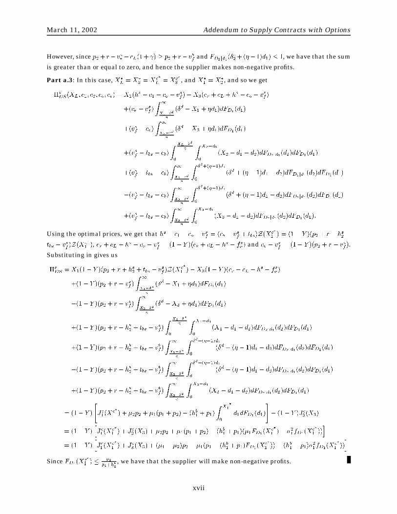
March 11, 2002 Addendum to Supply Contracts with Options
However, since p2+ r� vsr � cL(1+ ) � p2+ r� vbf and FD2jd1(Æc2+(�� 1)d1) � 1, we have that the sum
is greater than or equal to zero, and hence the supplier makes non-negative profits.
Part a.3: In this case, X�L = X�
3 = Xc�
L = Xc�
3 , and X�1 = X�
2 , and so we get
�sDS(XL; c1; c2; co; ce) = X1(h
s + c1 � co � vsf )�X3(cr + cL + hs � co � vsf )
+(ce � vsf )
Z 1
X1�Æd
�
(Æd �X1 + �d1)dFD1(d1)
+(vsf � ce)
Z 1
X3�Æd
�
(Æd �X3 + �d1)dFD1(d1)
+(vsf � tbs � cb)
Z XL�Æd
�
0
Z X2�d1
0
(X2 � d1 � d2)dFD2jd1(d2)dFD1(d1)
+(vsf � tbs � cb)
Z 1
X2�Æd
�
Z Æd+(��1)d1
0
(Æd + (� � 1)d1 � d2)dFD2jd1(d2)dFD1(d1)
�(vsf � tbs � cb)
Z 1
X3�Æd
�
Z Æd+(��1)d1
0
(Æd + (� � 1)d1 � d2)dFD2jd1(d2)dFD1(d1)
+(vsf � tbs � cb)
Z 1
X3�Æd
�
Z X3�d1
0
(X3 � d1 � d2)dFD2jd1(d2)dFD1(d1):
Using the optimal prices, we get that hs + c1 � co � vsf = (cb � vsf + tbs)Z(Xc�
1 ) = (1 � Y )(p2 + r + hs2 +
tbs � vsf )Z(Xc�
1 ), cr + cL + hs � co � vsf = (1 � Y )(cr + cL + hs � fsv ) and ce � vsf = (1� Y )(p2 + r � vsf ).
Substituting in gives us
�sDS = X1(1� Y )(p2 + r + hs2 + tbs � vsf )Z(X
c�
1 )�X3(1� Y )(cr + cL + hs � fsv )
+(1� Y )(p2 + r � vsf )
Z 1
X1�Æd
�
(Æd �X1 + �d1)dFD1(d1)
�(1� Y )(p2 + r � vsf )
Z 1
X3�Æd
�
(Æd �X3 + �d1)dFD1(d1)
+(1� Y )(p2 + r + hb2 + tbs � vsf )
Z X1�Æd
�
0
Z X1�d1
0
(X1 � d1 � d2)dFD2 jd1(d2)dFD1(d1)
+(1� Y )(p2 + r + hb2 + tbs � vbf )
Z 1
X1�Æd
�
Z Æd+(��1)d1
0
(Æd + (� � 1)d1 � d2)dFD2jd1(d2)dFD1(d1)
�(1� Y )(p2 + r + hb2 + tbs � vbf )
Z 1
X3�Æd
�
Z Æd+(��1)d1
0
(Æd + (� � 1)d1 � d2)dFD2jd1(d2)dFD1(d1)
+(1� Y )(p2 + r + hb2 + tbs � vbf )
Z 1
X3�Æd
�
Z X3�d1
0
(X3 � d1 � d2)dFD2jd1(d2)dFD1(d1)
= (1� Y )
"Jc1(X
c�
1 ) + �2p2 + �1(p1 + p2)� (hb1 + p1)
Z Xc�
1
0
d1dFD1(d1)
#+ (1� Y )Jc3(X3)
= (1� Y )hJc1(X
c�
1 ) + Jc3(X3) + �2p2 + �1(p1 + p2)� (hb1 + p1)(�1FD1(Xc�
1 )� �21fD1(Xc�
1 ))i
= (1� Y )hJc1(X
c�
1 ) + Jc3(X3) + (�1 + �2)p2 + �1(p1 � (hb1 + p1)FD1(Xc�
1 )) + (hb1 + p1)�21fD1
(Xc�
1 ))i
Since FD1(Xc�
1 ) � p1p1+hb1
, we have that the supplier will make non-negative profits.
xvii