Embed Size (px)
Citation preview
M.Sc. ThesisMaster of Science in Engineering
Coordinated Voltage Control of OffshoreWind Power and Multi-Terminal DC Grid
Rafael Calpe Domens (s161341)
Supervised by: Shaojun HuangKongens Lyngby 2018

DTU Electrical EngineeringDepartment of Electrical EngineeringTechnical University of Denmark
Ørsteds PladsBuilding 3482800 Kgs. Lyngby, Denmark
Tel: (+45) 45 25 38 [email protected]

SummaryIn this master thesis a Model Predictive Control is implemented for wind farm
voltage control purposes. Aiming at upgrading the voltage level at the POC bus whileimproving also the rest of bus voltages. This MPC is based on a optimisation problemincluding system dynamics along a time-horizon. Hence, taking the best control ac-tion for minimising voltage deviations along a series of predicted states of the network.
According to the voltage control state-of-the-art, this project can be sorted by thefollowing topics. It is a centralised park level controller based on system state opti-misation. Focusing on the voltage target is a time-horizon dependent control sincesome of its input information comes from estimated future information. Furthermore,it handles a series of technologies such as WTG-converters, OLTC transformers andHVDC-VSC. These are integrated and coordinated in several strategies under thesame scenario. Thus, working as a benchmark for further development of offshorewind power projects.
Along this work the following concepts are covered. First, an efficient voltage sen-sitivity technique is addressed analytically. Later on, this sensitivity is in charge ofquantifying voltage errors related to the predicted system states. Second, the optimi-sation problem is explained for each strategy covering each of the controlled devices.This minimisation integrates the decision variables associated with each technology,system measurements, system set-points, system dynamics (state space model) andso, the predicted voltage deviation related to those future dynamics. Moreover, op-erational constraints of each device and voltage boundaries are defined. All theseconcepts are integrated into an MPC Matlab algorithm. Third, this MPC controlleris modelled in DIgSilent PowerFactory providing the input for the controlled networkdevices. Then, carrying out a dynamic simulation for testing the performance of eachstrategy and technology. Finally, an extra strategy is set for further coordinationwith external network devices. Then, trying to bring some benefits to another gridwhile keeping optimal performance within the wind farm.

ii

ResumenEn este trabajo de fin de máster (TFM) un controlador de modelo predictivo
(MPC) es implementado para el control de voltaje en un parque eólico. En primerlugar, se trata de mejorar el nivel del voltaje en el nodo POC mientras se consigatambién una mejorar en el resto de nodos del parque. Este controlador MPC se basaen un problema de optimización que incluye las dinámicas de la red eléctrica a lolargo de un periodo de tiempo. Así pues, tomando las mejores acciones de controlpara minimizar la desviación del voltaje a lo largo del una serie de estados estimadosde la red.
De acuerdo al actual estado del arte de controladores de voltaje, este proyecto sepuede catalogar con los siguientes términos. Se trata de un controlador centralizadoa nivel de parque basado en la optimización del estado del sistema. Mientras su obje-tivo principal es la reducción del error del voltaje, dicho controlador es dependientedel tiempo ya que incluye en sus decisiones información de estados futuros. Además,maneja y coordina una serie de tecnologías como las turbinas eólicas, transformadoresy convertidores. Todos ellos integrados en diferentes estrategias y examinados bajoel mismo criterio. Por lo tanto, este proyecto pretende servir como referencia parafuturos desarrollos y estudios en proyectos de energía eólica offshore.
A lo largo del proyecto se cubren los siguientes conceptos. Primero, una eficaztécnica para calcular analíticamente coeficientes de la sensibilidad del voltaje. Mástarde, estos coeficientes se encargan de cuantificar los errores del voltaje relacionadoscon los estados del sistem predecidos. En segundo lugar, un problema de optimizaciónes explicado para cada una de las estrategias cubriendo cada uno de los dispositivoscontrolados. Dicha minimización integra las variables de decisión asociadas con cadatecnología, medición de la red, referencias del sistema y dinámicas del sistema. Entercer lugar, este controlador MPC es modelado en PowerFactory proporcionandola entrada para los dispositivos controlados en la red eléctrica. Posteriormente, cadatecnología y estrategia es evaluada mediante simulaciones dinámicas. Por último, unaestrategia adicional es definida para aumentar la coordinación con dispositivos de unared externa al parque eólico. De esta forma, tratando de aportar mejoras a otra redmientras se conserva el funcionamiento optimo dentro del parque.

iv

PrefaceThis Master thesis was prepared at the department of Electrical Engineering at
the Technical University of Denmark in fulfilment of the requirements for acquiringa Master of Science in Electrical Engineering, with study line in Electric EnergySystems.
Kongens Lyngby, February 27, 2018
Rafael Calpe Domens (s161341)

vi

ContentsSummary i
Resumen iii
Preface v
Contents vii
List of Figures ix
List of Tables x
Nomenclature xi
1 Introduction 11.1 EU Future Objectives . . . . . . . . . . . . . . . . . . . . . . . . . . . 11.2 New Power System Challenges . . . . . . . . . . . . . . . . . . . . . . 31.3 Grid Codes . . . . . . . . . . . . . . . . . . . . . . . . . . . . . . . . . 41.4 Master Thesis’ Objective . . . . . . . . . . . . . . . . . . . . . . . . . . 4
2 Voltage Control 72.1 Theoretical Principle . . . . . . . . . . . . . . . . . . . . . . . . . . . . 72.2 Literature review . . . . . . . . . . . . . . . . . . . . . . . . . . . . . . 82.3 Model Predictive Control . . . . . . . . . . . . . . . . . . . . . . . . . 102.4 Sensitivity Coefficients . . . . . . . . . . . . . . . . . . . . . . . . . . . 12
2.4.1 Sensitivity to Q Injections . . . . . . . . . . . . . . . . . . . . . 132.4.2 Sensitivity to Slack Bus . . . . . . . . . . . . . . . . . . . . . . 132.4.3 Sensitivity to Tap Changes . . . . . . . . . . . . . . . . . . . . 142.4.4 Sensitivity Analysis Results . . . . . . . . . . . . . . . . . . . . 15
3 Wind Farm Coordination 193.1 Wind Farm Voltage Control . . . . . . . . . . . . . . . . . . . . . . . . 19
3.1.1 Optimisation . . . . . . . . . . . . . . . . . . . . . . . . . . . . 193.1.2 State Space Model . . . . . . . . . . . . . . . . . . . . . . . . . 22
3.2 Wind Farm + OLTC Voltage Control . . . . . . . . . . . . . . . . . . 24

viii Contents
3.2.1 Optimisation . . . . . . . . . . . . . . . . . . . . . . . . . . . . 253.2.2 State Space Model . . . . . . . . . . . . . . . . . . . . . . . . . 26
3.3 Wind Farm + VSC-HVDC Voltage Control . . . . . . . . . . . . . . . 273.3.1 Optimisation . . . . . . . . . . . . . . . . . . . . . . . . . . . . 283.3.2 State Space Model . . . . . . . . . . . . . . . . . . . . . . . . . 29
3.4 Power Factory . . . . . . . . . . . . . . . . . . . . . . . . . . . . . . . . 313.4.1 Wind Farm Voltage Control . . . . . . . . . . . . . . . . . . . . 313.4.2 Wind Farm + OLTC Voltage Control . . . . . . . . . . . . . . 343.4.3 Wind Farm + VSC Voltage Control . . . . . . . . . . . . . . . 35
3.5 Results and Discussion . . . . . . . . . . . . . . . . . . . . . . . . . . . 363.5.1 Wind Farm Voltage Control . . . . . . . . . . . . . . . . . . . . 363.5.2 Wind Farm + OLTC Voltage Control . . . . . . . . . . . . . . 383.5.3 Wind Farm + VSC Voltage Control . . . . . . . . . . . . . . . 413.5.4 Discussion . . . . . . . . . . . . . . . . . . . . . . . . . . . . . . 42
4 Network Coordination 454.1 Wind Farm + External OLTC Voltage Control . . . . . . . . . . . . . 45
4.1.1 Optimisation . . . . . . . . . . . . . . . . . . . . . . . . . . . . 464.1.2 State Space Model . . . . . . . . . . . . . . . . . . . . . . . . . 48
4.2 Power Factory . . . . . . . . . . . . . . . . . . . . . . . . . . . . . . . . 484.3 Results and Discussion . . . . . . . . . . . . . . . . . . . . . . . . . . . 49
5 Conclusion 535.1 Future Work . . . . . . . . . . . . . . . . . . . . . . . . . . . . . . . . 54
6 Conclusiones 55
Bibliography 57
Appendix A 61
Appendix B 65

List of Figures1.1 EU Power Mix in 2000 and in 2015 [3] . . . . . . . . . . . . . . . . . . . . 11.2 Danish Wind Power Capacity and Share [6] . . . . . . . . . . . . . . . . . 2
2.1 MPC Time Description [28] . . . . . . . . . . . . . . . . . . . . . . . . . . 112.2 MPC Controller and System Integration . . . . . . . . . . . . . . . . . . . 112.3 Admittance Profile . . . . . . . . . . . . . . . . . . . . . . . . . . . . . . . 162.4 Voltage Profile . . . . . . . . . . . . . . . . . . . . . . . . . . . . . . . . . 162.5 Voltage Magnitude Sensitivity to WT10 VAR injection . . . . . . . . . . . 172.6 Voltage Magnitude Sensitivity to 1-p.u. Increment in VP OC . . . . . . . . 182.7 Voltage Magnitude Sensitivity to a Tap-Down Step . . . . . . . . . . . . . 18
3.1 VAR Capacity Curve of Type 4 WTG . . . . . . . . . . . . . . . . . . . . 223.2 AVR control of a OLTC transformer [36] . . . . . . . . . . . . . . . . . . . 273.3 VSC Control Scheme . . . . . . . . . . . . . . . . . . . . . . . . . . . . . . 303.4 Nordic32 Power System [40]: Single-Line Diagram . . . . . . . . . . . . . 323.5 Wind Farm Network: Single-Line Diagram . . . . . . . . . . . . . . . . . 333.6 Voltage Controller Scheme . . . . . . . . . . . . . . . . . . . . . . . . . . . 333.7 WTG Scheme . . . . . . . . . . . . . . . . . . . . . . . . . . . . . . . . . . 343.8 OLTC Scheme . . . . . . . . . . . . . . . . . . . . . . . . . . . . . . . . . 343.9 Wind Farm VSC Scheme . . . . . . . . . . . . . . . . . . . . . . . . . . . 353.10 Wind Farm Active Power Output . . . . . . . . . . . . . . . . . . . . . . . 363.11 WFVC: Voltage Magnitude at POC and MV buses . . . . . . . . . . . . . 373.12 WFVC: Voltage Magnitude and Reactive Power of WTGs . . . . . . . . . 383.13 WF+OLTC VC: Voltage Magnitudes . . . . . . . . . . . . . . . . . . . . . 393.14 WTGs: Voltage Magnitude & Reactive Power . . . . . . . . . . . . . . . . 403.15 WF+OLTC VC: OLTC Tap Change Detail . . . . . . . . . . . . . . . . . 403.16 WF+VSC VC: Voltage Magnitude at POC and MV buses . . . . . . . . . 413.17 WF+VSC VC: VSC WF-Terminal Outputs . . . . . . . . . . . . . . . . . 423.18 VC Comparison: Voltage Magnitude at POC and MV buses . . . . . . . . 433.19 VC Comparison: WT7 and WT8 Voltage Magnitudes . . . . . . . . . . . 43
4.1 External Distribution Network: Single-Line Diagram . . . . . . . . . . . 454.2 Variable Load:VAR consumption . . . . . . . . . . . . . . . . . . . . . . . 464.3 Voltage Control Scheme . . . . . . . . . . . . . . . . . . . . . . . . . . . . 49

4.4 Voltage Impact in Bus 1042 due to Variable Load . . . . . . . . . . . . . . 494.5 Voltage Profile within the WF . . . . . . . . . . . . . . . . . . . . . . . . 504.6 Voltage Profiles of Variable Load Network . . . . . . . . . . . . . . . . . . 504.7 Tap Position of OLTC2 . . . . . . . . . . . . . . . . . . . . . . . . . . . . 51
List of Tables3.1 VSC Parameters . . . . . . . . . . . . . . . . . . . . . . . . . . . . . . . . 303.2 Voltage Controller Error Comparison . . . . . . . . . . . . . . . . . . . . . 44
4.1 Voltage Profile Error Comparison . . . . . . . . . . . . . . . . . . . . . . . 51
1 Sample of Line Admittances of the WF . . . . . . . . . . . . . . . . . . . 612 Sample of Voltage Measurements at t70 . . . . . . . . . . . . . . . . . . . 623 Voltage Magnitude Sensitivity to Q Injections . . . . . . . . . . . . . . . . 634 Voltage Magnitude Sensitivity to VP OC . . . . . . . . . . . . . . . . . . . 64

NomenclatureAcronyms
AC Alternating Current
AV R Automatic Voltage Regulator
DC Direct Current
DSO Distribution System Operator
EU European Union
FACTS Flexible AC Transmission System
FRT Fault Ride Through
GW Gigawatts
HV High Voltage
HV DC High Voltage Direct Current
IEEE Institute of Electrical and Electronics Engineers
LV Low Voltage
LV RT Low Voltage Ride Through
MPC Model Predictive Control
MPPT Maximum Power-Point Tracking
MSE Mean Squared Error
MV Medium Voltage
MW Megawatts
OLTC On-Load Tap Changing
PCC Point of Common Coupling

xii List of Tables
PI Proportional-Integral Controller
PLL Phase Locked Loop
POC Point of Connection
PV Photovoltaic
QP Quadratic-Programming
RMS Root-Mean-Square
SV C Static VAR Compensator
TSO Transmission System Operator
V AR Volt-Ampere Reactive
V SC Voltage Sourced Converter
WP Wind Power
WT Wind Turbine
WTG Wind Turbine Generator
Symbols
∆udint Internal Control Voltage Magnitude Increment
∆idP I PI-controller Current Increment
∆ntap Tap Step Increment
∆nreftap Tap Step Reference Increment
∆Q Reactive Power Increment
∆Qref Reactive Power Reference Increment
∆Td Discretisation Period
∆Tp Prediction Period
∆ud_refs Voltage Magnitude Reference Increment
∆uds Voltage Magnitude Measurement Increment
∆V Voltage Increment
∆V pre Predicted Voltage Error
N Set of Buses in the network

List of Tables xiii
S Set of Slack Buses in the network
Re Real Part of a Number
θ Phase
Cf Filter Capacitance
I Current
ko_i VSC Outer-loop Integral Gain
ko_p VSC Outer-loop Proportional Gain
NB Number of Buses in the network
Nc Number of Control Steps
Np Number of Prediction Steps
Ns Number of Predictions in each Control Step
NW Number of WTG Buses in the network
P Active Power
P av Available Wind Power
P ext External Active Power from WTG
P dm VSC d-axis Modulation Index
P qm VSC q-axis Modulation Index
Q Reactive Power
R Resistance
S Apparent Power
Tc Control Period
Td VSC Time-constant Delay
Tp Prediction Horizon
Tinr VSC Inner-loop Time-constant Delay
ud d-axis Voltage
uq q-axis Voltage
V Voltage

xiv List of Tables
V ref Voltage Reference
V th Voltage Threshold
X Reactance
Y Admittance
Ybus Admittance Matrix
Z Impedance

CHAPTER 1Introduction
1.1 EU Future ObjectivesOnce climate change was recognised as a fact through the Kyoto Protocol, the Eu-
ropean Union (EU) set several energy strategies for next decades in order to tackle it.Some targets must be achieved by 2020 and 2030 in order to reduce greenhouse gases.Among them, it is highlighted a 20% of minimum renewable energy contributionin the total electricity consumption by 2020 [1]. Thus, promoting the investment innew sustainable sources of energy production instead of conventional fossil fuel power.
Some other governments, such as the Danish, went a step further on their climatepolicies. In this case, aiming at a 30% of renewable production to supply its totalenergy consumption for the same date as before stated [2].
Figure 1.1: EU Power Mix in 2000 and in 2015 [3]
This framework pushed up the growth of renewable sources’ share as it can beseen in Figure 1.1. The total power capacity was increased from a 24% to a 44%.
2 1 Introduction
A promising jump backed up by the policies mentioned before, even they were onlycommitted from 2008 on.
Moreover, a deeper analysis of renewable sources can be done. This suggests ahuge development of wind energy. Firstly, it stands as the power source which morehas increased its capacity, with almost 130 GW installed along that period. Evenmore than the natural gas. Secondly, it beats hydro power and gets its historic firstposition as the main renewable energy source. Later on, figures from 2016 provideseven further success. While an 86% of new power installations are of renewablesources, more than the half of them are related to wind energy. In addition, windpower defeated coal in the capacity power mix [4]. It means that wind power repre-sents the second largest source of energy of the whole EU.
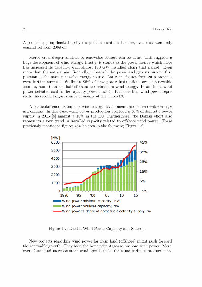
A particular good example of wind energy development, and so renewable energy,is Denmark. In this case, wind power production overtook a 40% of domestic powersupply in 2015 [5] against a 10% in the EU. Furthermore, the Danish effort alsorepresents a new trend in installed capacity related to offshore wind power. Thesepreviously mentioned figures can be seen in the following Figure 1.2.
Figure 1.2: Danish Wind Power Capacity and Share [6]
New projects regarding wind power far from land (offshore) might push forwardthe renewable growth. They have the same advantages as onshore wind power. More-over, faster and more constant wind speeds make the same turbines produce more

1.2 New Power System Challenges 3
energy. For this reason, bigger wind turbines and larger wind farms are topics of in-terest. Among those, it can be found wind farms of the same capacity of conventionalpower plants. Thus, satisfying both reduction of greenhouse gas emission and raisingthe share of sources of green energy. What helps speeding up the decarbonisationprocess established at the EU objectives.
1.2 New Power System ChallengesAs it has been shown in the previous section, the renewables have been pushed
forward due to environmental policies and a sustainable attitude. However, it is notall about good actions installing renewables all around. It challenges the power sys-tem, the actual structure which is holding up the changes regarding electric energygeneration.
Historically the power system has been a network connecting generators of elec-tricity to customers through transmission and distribution grids. A model which wasdefined as centralised. Based on large power plants settle down close to their sourceof energy such as coal mines or harbours importing oil and gas. They were sendingenergy far away to the points of consumption. Moreover, the flow of energy was strictto only one-direction: generation – transmission – consumption.
The first challenge comes up with utility-level renewable sources such as windfarms and photovoltaic (PV) solar farms since they can be installed closer to thepoints of consumption. What means that power losses are lower even if they are notsent at really high voltages. Thus, large step-up transformers and high voltage linesare not needed for this new configuration.
Second, a new agent is defined as ‘prosumer’ who threats the one-direction estab-lished rule. This customer of energy is connected to the distribution grid, as usual.However, this new agent has a new function which is generating energy with forexample PV panels. Depending on their consumption and generation, they can beeither a traditional sink or otherwise, a source of electricity. A fact which causesmodifications on power flow directions and voltage profiles of the network.
The third and more critical issue regards power system operation. For so longtime, conventional generators were set to follow a constant power reference accordingto the energy demand at that moment. Consumption patterns are predictable andthey are calculated with certain accuracy. However, renewable sources can not followa set-point all the time. The most important drawbacks are their uncertainty andvariability. The former one makes it extremely difficult to forecast their instantaneousmaximum production, so their power share to the system. The latter makes troubleon real-time operation. Continuous variations on weather conditions make fast and

4 1 Introduction
large changes on energy injections. For these reasons, fast conventional generatorsare still needed as backup of the system to meet production and consumption levels.
These issues are only some of the actual concerns of the electricity system andall their agents involved in. In spite of these challenges, the network must provideelectricity of quality to the points of consumption. For this reason, the grid codeswere created. They set the requirements of the power supply in order to ensure agood quality energy service.
1.3 Grid CodesGrid codes can be defined as a framework of technical regulations which ensures
a secure power system performance in order to supply good quality energy to theconsumption points. Each Transmission System Operator (TSO) rules all the agentsconnected within the same network, from generators to customers.
As system performance depends on many agents and their electric parameters atthe point of connection, a series of secondary services are classified as ancillary servicesaccording to each technical parameter addressed [7]: scheduled power generation, fre-quency/active power control, voltage/reactive power control, inertial response, faultride through, fault current contribution, etc.
Among these regulations, frequency and voltage might be the most importantparameters to take into account. The former one characterises the whole system fre-quency and represents all the synchronous elements working in a specific area. Thelatter one states the set-point at each system level in order to provide a good qualityservice to each consumer. For that reason, they were the minimum requirements atthe point of connection (POC) that a renewable energy producer had to satisfy someyears ago.
However, the regulations and minimum requirements are changing along the timedue to a challenging increment of share of renewables. As more conventional powerplants are closed, there are less agents providing ancillary services for a secure sys-tem. Moreover, there are more variations on generation and so, more risk of systemdisturbances. Therefore, more services and more strict requirements are now askedto renewable energy producers.
1.4 Master Thesis’ ObjectiveFirst of all,this project is an extension of the research study carried out in [8].

1.4 Master Thesis’ Objective 5
As it is stated previously, offshore wind farms are a current spotlight becauseof its potential. They can supply larger amounts of power to the grid in order tofurther increase the share of renewables even substituting conventional power plantof large size. However, they represent a big challenge for the energy sector. First,larger amounts of power mean higher voltage variability and stability issues withinthe wind farm. Second, these effects are transmitted into the system. So the wholesystem might reflect the voltage fluctuations.
For those reasons, this work aims at improving the performance of wind farms totackle those challenges while pushing forward wind power development. Specifically,the main target of this work is the voltage control of all the buses related to thewind farm. Firstly, designing a voltage control to keep all the buses in the windfarm within limits, so that all the wind turbine generators (WTG) are working ina safe state. Secondly, analysing and coordinating new technologies to enhance theperformance of the whole wind farm at the POC. Thirdly, coordinating the voltagecontrol of the wind park with other main network devices to improve the behaviourof the main network while keeping an optimal state of the wind farm.

6

CHAPTER 2Voltage Control
2.1 Theoretical PrincipleA constant voltage is desired across all the nodes of a power system in order to
provide a good quality electricity service to final customers. Moreover, that wouldmean all electrical machines and auxiliary devices are within their safety limits andclose to their respective rated value. Thus, everything would be working safely andensuring optimal operational performance. However, this ideal state is difficult toachieve due to the massive amount of interconnected devices in a network and theirdifferent dynamics. For this reason, controlling the voltage is a major concern inpower system operation. Even more, with the new challenges already introduced be-fore.
Nonetheless, ensuring the right voltage level in a grid means a deep understandingof electrical parameters. First of all, the variables which determine that level must befound. Later on, controlling their influence will be the second objective. Therefore,an analysis of the voltage parameter is developed in the following equations. Anapproach to the basics is carried out with a simple example [9]. In this case, thepower transfer S = P + j · Q between two points A and B in a single line circuit isanalysed through an impedance Z = R + j · X.
SB = VB · I∗ = P + j · Q (2.1)
VA = VB + (R + j · X) · I = VB + (R + j · X) ·(P − j · Q
V ∗B
)(2.2)
∆V = VA − VB ≈ ∆Vreal = R · P + X · Q
VB(2.3)
Based on Equation (2.1) and its the complex power S from the receiving B pointof view, Equation (2.2) develops the voltage at the source A end. Taking into accountan assumption for distribution circuits, the phase δ of the voltage is small and can beapproximated to zero. Then, VB = V ∗
B = |VB |. Eventually, including this assumptioninto Equation (2.2) allows developing the equation and split it into real and imaginaryparts. Being the latter part approximate to zero because of the distribution circuitassumption again. Finally, the voltage increment ∆V between two nodes is presented
8 2 Voltage Control
in Equation (2.3).
Next, the variables which influence the voltage can be analysed. According to(2.3), the voltage at a bus depends on two aspects. First, its reference level or di-rectly linked bus due to the connection itself. Second, a couple of variables whichdepends on the power transfer and hence, on the active P and reactive power Q de-manded on a load at the receiving terminal. Active power is not considered in thisanalysis since it is assumed as fixed due to two reasons. Firstly, in the case of aload its operation depends directly on P , then a right behaviour is not pretended tobe compromised. Secondly, in the case of a source such as a wind farm its revenuedepends on the active power injected and hence, it is maximised to actual weatherconditions and non-control is expected. Consequently, reactive power takes over theresponsibility as the variable for voltage variation.
For this reason, reactive power stands out for being in charge of the primary volt-age control as suggested in [10]. It is considered as a local problem of an area andhence, a reactive power balance must be kept across the devices within this area.These devices can be gathered in two groups: sources or sinks of Q. The formergroup joints the following devices: overexcited synchronous generators, shunt capaci-tors banks, capacitances of overhead lines and cables and, Flexible AC TransmissionSystems (FACTS). On the other hand, the sinks are the following: underexcitedsynchronous generators, inductive motors and loads, shunt reactors, inductances ofoverhead lines, cables and transformers and, FACTS. Furthermore, the last wind tur-bine models such as type 3 and type 4 also provides reactive power support with theirconverter technology. Reactive power capability which can work in any of the groupspresented. It is justified by a series of control modes or controller diagrams suggestedin [11] in order to emulate the automatic voltage regulator (AVR) of conventionalsynchronous generators.
2.2 Literature reviewVoltage control has been studied for a long time and hence, a wide range of
topics are covered in its state-of-the-art. Although decentralised or machine levelcontrollers were of interest, this research study is focused on wind farm voltage con-trol level. Within this area, a long classification of techniques is described as follows.First, voltage analysis can be subdivided into controllers and optimisation. Second,the time-horizon of different methods is suggested. Third, a series of objectives arecovered. Fourth, voltage or VAR support is sorted by controlled devices.
First of all, voltage controllers for park level are usually a PI emulating the AVRof a traditional machine as suggested in [12, 13]. They can integrate features likedrop compensation or feedback loops as presented in the former source. Otherwise,the latter one proposes a coordination of different hierarchical levels of controllers

2.2 Literature review 9
for faster actions. While all these controllers are implemented for fixed real-timepurposes, [14] introduces a series of controllers which are shifted depending on thestate of grid parameters. Thus, proposing a series of control strategies joint underthe term VAR optimisation method. Later on, more advanced designs have evolvedinto optimisation algorithms gathering different time-scales, objectives and devices.
Secondly, the time-horizon is a control parameter to take into consideration. In[15, 16], VAR control strategies are dependent on the time frame. From millisecondsto seconds, the objectives are low voltage or fault ride through (LVRT or FRT). Fromseconds to minutes, it addresses voltage stability, power factor or flicker mitigation.Then, for longer periods the strategies are VAR support to the system or power lossminimisation. On the other hand, time-dependent parameters such as wind speed orconsumption load are considered in the study of [17]. It analyses the benefits of intro-ducing forecast data of those variables in the optimisation. However, the results showthat if a perfect knowledge of the variables is not available, the performance is similarto a simple voltage controller. Hence, [18] takes a different approach. It suggests anhourly optimisation which provides the reference for the wind power plant controllerfor that time. An extreme application of this long-time voltage control calculation isstudied in [19] for planning purposes. Therein, the allocation of VAR-support devicesis assessed.
Thirdly, an optimisation algorithm can be in charge of different objectives. Whilethe voltage control is considered the main one for this project, secondary targetsmight bring some benefits for the wind farm. From the more basic power factorcontrol in [14], then a maximum power-point tracking (MPPT) in [20] and even theeconomically evaluation from [19, 21]. On the other hand, a more often goal is thepower loss reduction which is reviewed in [18, 20, 22, 23].
Fourthly, the device taking over the VAR support is another factor. Based onthe VAR contribution of WTGs, auxiliary electrical machines are integrated in thevoltage control. The reactive power supply is enhanced by a static VAR compensator(SVC) in [16, 20, 22]. Network topology is modified by an OLTC transformer in [17,22]. Furthermore, a decoupled network connected through HVDC is applied in [24,25]. In this case, the voltage control is carried out by their converter which handlesthe voltage of the DC-link. Then, introducing a coordination among the devices con-nected to that multiterminal DC grid.
Further coordination is explained in [26]. It develops an optimisation algorithmwith some of the previous methodologies explained above. That is a voltage controlbased on an incremental linear problem adjusting VAR responses to minimise powerlosses. Also, coordinated responses from WTGs, an OLTC and an SVC. Furthermore,it introduces a technique based on sensitivity coefficients for integrating power systeminfluences. Thus, being this example an approach to the MPC method explainedbelow and carried out along the project.

10 2 Voltage Control
2.3 Model Predictive ControlModel predictive control (MPC) is an advanced control technique which has been
used for long time in manufacturing and processing industries [27]. More recently, ithas been extended to power systems and other subsystem networks [28]. Its main fea-ture is gathering three principles: modelling, prediction and optimisation. Firstly, anapproximate linear model represents the dynamics of every element of the system atthe same time that it integrates influences among the subsystems. Secondly, the con-trol problem includes a fixed interval of time and it is solved along the time-horizon.For this reason, this method takes into account the behaviour and long-term effect ofthe model over the finite-horizon. Thirdly, the control actions are decided accordingto an optimisation problem. Thus, an optimal solution is found for each time step,although only the first control action is applied and kept along that control period [29].
It is suitable for power system control because of the following advantages. First,its dynamic model captures both fast and slow responses of the systems. Thus, acoordination between devices is feasible. For instance, the relatively fast responseof WTG converters can be integrated to slow tap changes of transformers, takinginto consideration the long-term effects of each one. This system modelling layson the state space model from Equation (2.4). Second, the optimisation problemallows flexibility. In this project, a voltage control strategy has been pointed out. Itjoins different voltage targets across the network. However, a multi-objective functioncould also have been implemented in order to reduce system losses or operational cost.Third, this kind of problem again stands out due to its ability to handle constraints.A key aspect to capture real performance of the machines taking into account eithertheir operational limits or grid operational requirements. An optimisation problemcan be seen in (2.5), where both objective function and constraints are described.
x = A · x + B · u
y = C · x(2.4)
minNp∑
k=1
(ε2(V ))
Subject to : Vmin < V < Vmax
(2.5)
Once the working principle and advantages of the MPC have been presented, thetime-domain variables must be clarified for deeper understanding. These variablesare: the prediction horizon Tp, the control period Tc and the prediction period ∆Tp.They are sorted from bigger to smaller time duration. Their selection must be carefulsince the accuracy of the whole control depends on them. Therefore, the predictionhorizon must gather all the long-term effects of the subsystem and the predictionsteps must follow the fast dynamics of the machines. Instead of time duration, theyalso can be identified as number of steps along the prediction horizon as follows: the

2.3 Model Predictive Control 11
number of predictions in each control step is Ns = Tc
∆Tp, there are the following con-
trol steps Nc = Tp
Tc, then the total number of prediction steps is Np = Tp
∆Tp. The
time-domain variables meaning can be found in Figure 2.1 as a example.
Figure 2.1: MPC Time Description [28]
Regarding the MPC application, a methodology for integration is illustrated inFigure 2.2. On the left side, an MPC algorithm is implemented in a software such asMatlab while reading both references and measurements of actual operation of thesystem. On the right side, the power system with its devices (machines, controllersand sensors) are implemented. Finally, a communication is needed between both sidesfor a feedback control implementation. Along the project both parts, algorithm andsystem model are explained more in detail.
Figure 2.2: MPC Controller and System Integration

12 2 Voltage Control
2.4 Sensitivity CoefficientsSensitivity coefficients are used in power system control to relate control vari-
ables to controlled parameters based on linear-model approaches. It helps an algo-rithm such as the MPC to aggregate the current and/or predicted effects of controlvariables with their affected grid parameters. As it is suggested in [30], the traditionalmethod consists of updating the Jacobian matrix of the load flow analysis. However,this approach has two drawbacks. First, the computational burden and processingtime. This method updates the Jacobian for each iteration according to the currentstate of the network. What means building and inverting a matrix of the size of thenetwork. Second, this technique does not provide a unique solution for each iteration.Furthermore, neither Newton Raphson nor fast decoupled load flow methods find aconvergent solution for this problem as it is explained in [31]. For these reasons, theJacobian approach does not seem convenient for real-time applications and the firstsource proposes a new methodology.
It must be highlighted that the scope of those research studies is radial distribu-tion networks. This kind of grid is characterised by its high R/X ratio. In spite ofthat fact, a similar structure is found on the radial structure and long MV feeders(high R/X ratio) of traditional wind farms. Thus, those study results are consideredof interest and hence, their proposals are implemented in this project. Further on, itis justified by the use of this calculation method in similar wind farm research studiessuch as [8], [28] and [32].
Eventually, the application of this computational efficient method, and specificallyin the wind farm case, is based on a series of assumptions. Considerations neededfor backing up the mathematical development shown below and its unique solutions.Thus, they must be emphasised even though some have been already commented.
• Slack bus voltage magnitude and angle remain constant independently of thepower injections
• PQ injections are considered constant and independent of bus voltages
• While there is a PQ injection change in a bus, all the other power injectionsremain constant
• The partial derivatives showed have a unique solution for every radial distribu-tion network
• The wind farm network is considered as radial distribution network due to itstopology

2.4 Sensitivity Coefficients 13
2.4.1 Sensitivity to Q InjectionsAs one of the main targets of this project is a coordinated wind farm voltage
control, the sensitivity coefficient of interest is related to the voltage magnitude. AsWTGs are one of the technologies controlling the voltage, their reactive power effectover the voltage magnitude must be demonstrated. The efficient analytical computa-tional method demonstrated by [30] is explained in the following lines starting withthe relationship between complex power S and complex voltage V .
Si = Vi ·∑j∈N
(Ybus(i, j) · Vj) (2.6)
Where Si and Vi are the conjugates of their respective complex numbers, Ybus isthe admittance matrix of the network and, i and j are bus identifiers which belongto the set N = {1, 2, . . . , NB}. Where NB represents all the buses of the wind farm.
Next, the derivation of the voltage in regards to the VAR injection in a bus l ∈ Nis carried out in Equation (2.7). This suggested calculation provides a linear equationto the unknown voltage derivative variables. Moreover, it has a unique solution forthe radial distribution network assumption. This solution is equal to ’−j1’ when i = land, ’0’ for the rest of cases.
∂Si
∂Ql= ∂{Pi − jQi}
∂Ql= ∂Vi
∂Ql·
∑j∈N
(Ybus(i, j) · Vj) + Vi ·∑j∈N
(Ybus(i, j) · ∂Vj
∂Ql
)(2.7)
Later on, a system of equations is set individually with the real and imaginarypart of the previous equation and its solutions. Besides, two principles are needed fortheir development. First, the derivative of the conjugate of a complex number is equalto the conjugate of the derivative of that complex number. Second, the equations ofCauchy−Riemann are implemented. This procedure provides the value of the partialderivatives associated with voltage sensitivity. Finally, the desired voltage magnitudesensitivity to VAR injection is calculated with the following equation.
∂|Vi|∂Ql
= 1|Vi|
·Re(
Vi · ∂Vi
∂Ql
)(2.8)
2.4.2 Sensitivity to Slack BusAs voltage magnitude is the main goal of the analysis, it must be related to dif-
ferent parameters. Once the reactive power has been explained as a voltage influenceagent, the voltage change of a reference bus is indeed another one. It must be, ofcourse, a strong or reference bus to make a considerable modification. For this reason,the second agent of influence is the voltage magnitude change in an assumed slackbus. The analysis starts again in Equation (2.9) with the relationship between the

14 2 Voltage Control
conjugates of complex power Si and complex voltage Vi. Now, S is the set of slackbuses which respects this assumption: S ∪ N = {1, 2, . . . , NB} and S ∩ N = ∅.
Si = Vi ·∑
j∈S∪N(Ybus(i, j) · Vj) (2.9)
Then, the partial derivative with respect to the voltage magnitude of the slackbus is developed as shown in Equation (2.10). This voltage magnitude belongs to:Vk = |Vk| · ejθk , where the reference or slack bus k ∈ S and the solution of the
derivation is: ∂Si
∂|Vk|= 0.
∂Si
∂|Vk|= ∂Vi
∂|Vk|·
∑j∈S∪N
(Ybus(i, j) · Vj) + Vi ·∑
j∈S∪N
(Ybus(i, j) · ∂Vj
∂|Vk|
)(2.10)
Taking into account the following specific term for the slack bus:
∂
∂|Vk|∑j∈S
(Ybus(i, j) · Vk) = Ybus(i, k) · ejθk (2.11)
previous Equation (2.10) and its solution can be formulated as:
−Vi · Ybus(i, k) · ejθk = ∂Vi
∂|Vk|·
∑j∈S∪N
(Ybus(i, j)) · Vj + Vi ·∑j∈N
(Ybus(i, j) · ∂Vj
∂|Vk|
)(2.12)
Eventually, this equation is linear in regards to voltage partial derivatives accord-ing to the methodology suggested in [30]. Partial derivatives which are the unknownsof a system of equations with a unique solution for the assumed radial distributionnetwork or wind farm in this case. Therefore, the sensitivity solution is the followingEquation (2.13). But the target of this section is voltage magnitude sensitivity tovoltage magnitude change of the slack bus, so only the real part is of interest lateron and it is shown in Equation (2.14).
∂Vi
∂|Vk|=
( 1|Vk|
· ∂|Vi|∂|Vk|
+ j · ∂θi
∂|Vk|
)· Vi, ∀i ∈ N (2.13)
∂|Vi|∂|Vk|
= |Vi| · Re( 1
Vi· ∂Vi
∂|Vk|
)(2.14)
2.4.3 Sensitivity to Tap ChangesAn OLTC is considered also an agent of influence on the voltage. It makes a
direct effect into the voltage magnitude, which is the main target of the sensitivity

2.4 Sensitivity Coefficients 15
analysis carried out along this section. This effect is related to a tap position incre-ment ∆ntap. For this reason, the voltage magnitude change due to a tap step mustbe quantified with the following explanation.
Each tap transformer change is strongly related to the voltage magnitude changein the slack bus presented in previous section. Therefore, all the previous equationdevelopment is useful as well in this coefficient analysis. Taking into account thatthe HV-side terminal of the OLTC is now the assumed slack bus k. Then, Equation(2.15) introduces the sensitivity to a tap position change.
∆|Vi|∆ntap
= ∂|Vi|∂|Vk|
· ∆Vtap (2.15)
Where the first term of partial derivatives corresponds to the results from Equa-tion (2.14). In addition, ∆Vtap is the voltage magnitude step related to each tap step.What is considered as a main feature set by the transformer manufacturer and in thiscase is equal to 1.25% of the rated voltage in each terminal.
Eventually, a couple of considerations regarding the tap change sensitivity. Firstly,it is considered as a discrete magnitude due to its discrete tap positions. Secondly,the voltage magnitude step effect is expected to happen only in the LV-terminal ofthe OLTC due to the electrical coupling of the HV-side with the main network.
2.4.4 Sensitivity Analysis ResultsThe sensitivity coefficients calculated depend directly on two aspects. First, the
network topology which is kept constant in a simulation. Second, the current state ofthe system measured through the bus voltages. Since the latter one is changing all thetime, a random calculation is chosen as an example. Thus, the results shown belowcorresponds to the system state at 70 seconds of a simulation which is explained later.In Figures 2.3 and 2.4 both parameters, topology and voltages are illustrated. In thiscase, one of the four feeders (from WT8 to WT10) of a wind farm has been chosenas an example. For further detail about the Ybus or the voltage measurements of thisexample, they are in Tables 1 and 2 in Appendix A.
First of all, the sensitivity to reactive power injections is calculated following theguidelines presented above. The system of equations resolution is shown in AppendixB through a script. Solving this system of equations developed from Equation (2.7),the sensitivity of complex voltage to Q injections is found. Then, this solution isintroduced in Equation (2.8). Thus, the results of this equation are the expected sen-titivity of voltage magnitude to Q injections. The complete set of results for each busis shown in Table 3 in Appendix A. However, a brief visual results can be observedin Figure 2.5. There, the voltage magnitude changes according to 1MV Ar of changein WT10. In the upper part, the feeder of this wind turbine is represented together

16 2 Voltage Control
Figure 2.3: Admittance Profile
Figure 2.4: Voltage Profile

2.4 Sensitivity Coefficients 17
with the main buses of the WF. Below, another feeder of WTGs is shown to give anexample of how a single WTG influences all the other voltages.
Secondly, the voltage magnitude sensitivity to voltage magnitude change of thereference bus is calculated. Following the same procedure, a system of equation is setfrom Equation (2.12). This is also explained through the Matlab code in Appendix B.The solution of this system provides the derivative term needed in Equation (2.14).Next, the desired coefficients are found. These coefficients represent the rate of changeof voltage magnitude in each bus according to the voltage magnitude change in thereference bus (POC). Method used for instance for a HVDC-converter control. Someadjustment is needed for a good comprenhension of these parameters. In this caseAdjustment 1 calculates these coefficients divided by the ratio given for the POC bus.Then, getting the rate of change in each bus for a unity change in the reference. Asample of the results are illustrated in Figure 2.6 for the main MV collector bus andfor the WTGs of the second feeder of the WF. Further detail with all the coefficientsis stated in Appendix A.
Thirdly, the sensitivity to OLTC tap changes is worked out. In this case, thecoefficients are related to the previously calculation since they are also due to voltagechanges. For this reason, the same procedure is carried out in order to find theparameters. However, a different adjustment is needed this time. Assuming a strongcoupling of the POC bus to the external network, non reaction is going to be foundin the HV-side of the OLTC. Therefore, this value must be set to zero and its ratiomust be added to the rest of nodes with the opposite direction effect. The results ofthe adjustment (Adjustment 2) are gathered in Appendix A with the previous ones.Nonetheless, the direct coefficients of a tap change are found multiplying those voltage-
Figure 2.5: Voltage Magnitude Sensitivity to WT10 VAR injection

18 2 Voltage Control
Figure 2.6: Voltage Magnitude Sensitivity to 1-p.u. Increment in VP OC
change values by the voltage increment of each tap step, according to Equation (2.15).A sample of these coefficients at some of the buses are illustrated in Figure 2.7.
Figure 2.7: Voltage Magnitude Sensitivity to a Tap-Down Step

CHAPTER 3Wind Farm
CoordinationOnce a MPC has been chosen as a voltage control technique, the reactive power
capability of WTGs is going to be presented as the first strategy. After, a coordinationwith other devices is explained in this chapter, aiming at better behaviour of busvoltages profile. In the previous research work, a wind farm was coordinated withan automatic OLTC transformer and a static var compensator (SVC). Now and asa second strategy a controllable tap transformer is analysed to dismiss the need offast and expensive VAR devices such as the SVC. Besides, the increasing attention inhigh voltage direct current (HVDC) cables makes it a topic of interest for integratingthem into the voltage control framework as the third strategy. Eventually, it mustbe clarified that the MPC voltage control is implemented as a function in Matlab.On the other hand, the network topology and physical controllers are implementedin DIgSILENT Power Factory, while a communication between the two softwares isneeded.
3.1 Wind Farm Voltage Control
3.1.1 OptimisationAs it is stated in Section 2.3, the optimisation is one of the parts of the MPC.
At this stage, a decision-making process is carried out in order to decide the controlactions needed for the following prediction horizon. Even though, only the first con-trol action is applied. The main components of this methodology are the measuredvariables, the decision variables, the objective function and the constraints.
First, the measured or controlled variables. They are the network parameters tocare about, so the deviation concerning their reference need to be minimised. At thesame time, they are working as a flag. The MPC works in two control modes andthese network measurements determine which mode is active at each iteration. Thevoltage measurements are the following:

20 3 Wind Farm Coordination
• VP OC : Voltage at POC or high-voltage side of the OLTC
• VMV : Voltage at Medium Voltage bus or low-voltage side of the OLTC
• VW T : Array of voltage at wind turbine terminals
Regarding the voltage control modes, the first mode or CorrectiveMode takescare of all the controlled parameters. For this reason, if any of them overcomes itsthreshold, this mode is activated. In this way, every time there is a violation ofany of the controlled variables the MPC tries to improve the voltage profile of thewhole wind farm. At the same time it avoids wind turbine tripping. Then, its ob-jective function explained below takes action. The second mode or PreventiveModehowever, only takes care of the voltage at the POC. In this way, there is a furtherimprovement of the main parameter of the wind farm to its common reference, sincethe requirements from the system operator aim at this bus. That means preventionat the main bus while all the others are working within safe voltage ranges.
Usually, the voltage magnitude reference of all the buses are considered as V refi =
1p.u.. Regarding their thresholds, they are individual to keep individual targets orsafety ranges. First, at the POC the threshold is V th
P OC = 0.01p.u. due to its im-portance to system requirements. However, it depends on the grid code and systemoperator instructions. Second, V th
MV = 0.03p.u. due to more relaxed conditions withinthe wind farm. Third, V th
W T = 0.08p.u. since wind turbine protections are usually inthe range of [0.9, 1.1]. In this way, there is still a security gap before tripping out themachine.
Second, the decision variables are the solution of the optimisation. They providethe input for the devices controlled. Specifically, in this first strategy the decisionvariable is: ∆QW T , an array of the reactive power supply increment of each windturbine generator.
Third, there is a objective function (ObjFun: (3.1)). It consists of a minimisationsince the voltage deviation from the voltage reference wants to be reduced. In thiscase, a quadratic error function along the whole prediction horizon has been chosenfor two reasons. Firstly, it minimises the error penalising much more big deviationsfrom the set-point. Secondly, it takes into account the future states of the devices. Forthis reason, it tries to minimise the error along the long term, i.e. avoiding oscillationsdue to different dynamic responses from different devices. For this first strategy, theprediction horizon Tp is considered as 5 seconds to capture fast dynamics of WTGsfor a while. The control period Tc is 1 second and the prediction period ∆Tp is 0.5seconds.
min∆QW T
Np∑k=1
(∥∆V preP OC(k)∥2 + ∥∆V pre
MV (k)∥2 + ∥∆V preW T (k)∥2) (3.1)

3.1 Wind Farm Voltage Control 21
This objective function belongs to the CorrectiveMode. On the other hand, thePreventiveMode only has the first term of the equation regarding the predicted volt-age error at the POC. Another feature of the equation is that it can be weighted. Inthat case, each term would be multiplied by different values giving less importanceto the higher value during the optimisation process. For this project, all the voltageshave been considered with the same importance, so the same weight is considered foreach term. The development of each term of Equation (3.1) is explained here:
∆V preP OC(k) = VP OC(k) − V ref
P OC + ∂|VP OC |∂QW T
· ∆QW T (k) (3.2)
Where VP OC is the current voltage magnitude measurement before starting theMPC calculation, ∂|VP OC |
∂QW Tis the sensitivity coefficient array of the voltage magnitude
change at POC regarding a change of reactive power supply from each wind turbinegenerator and, ∆QW T states the decision variable array to be minimised.
∆V preMV (k) = VMV (k) − V ref
MV + ∂|VMV |∂QW T
· ∆QW T (k) (3.3)
∆V preW T (k) = VW T (k) − V ref
W T + ∂|VW T |∂QW T
· ∆QW T (k) (3.4)
Where each of the terms have the same meaning as in Equation (3.1) but now,they are referred to the MV Medium Voltage bus and the 20 WT wind turbine nodes.
Fourth, the constraints of the optimisation problem. Capturing the operationallimits of the electrical machines will provide a closer image of the actual performanceof the system. For this reason, the reactive power capability of the wind turbinegenerators has been implemented in the model as it is shown here:
QminW Ti
(k) ≤ QW Ti(k) ≤ Qmax
W Ti(k)
∀i ∈ [1, 20], k ∈ [1, Np](3.5)
Where QW Tiin the discrete form can be related to the decision variables as:
QW Ti(k) = ∆QW Ti
(k) + QW Ti(t0). Regarding the minimum and maximum values of
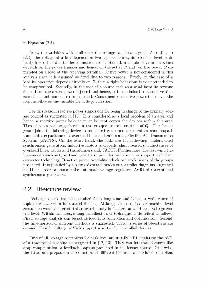
the reactive power of each wind turbine generator, they can be calculated as follows.The VAR capacity of each machine depends on its voltage terminal set by the networkand on the active power available in the machine, which at the same time dependson the wind power available. For that reason, the VAR limits are approximated bylinear interpolation of the current measurements to a look-up table which might beprovided by the machine manufacturer. An example can be seen in Figure 3.1
22 3 Wind Farm Coordination
Figure 3.1: VAR Capacity Curve of Type 4 WTG
In addition, three more constraints are needed for the right behaviour of themethod and the consideration of the control mode. If the MPC is working inPreventiveMode, the three following equations must be included as they are pre-sented. Otherwise, in the CorrectiveMode they are conditional. Depending on whichthreshold has been violated, these conditional constraints will be considered or not.Thus, they are only included if the voltage magnitudes are within range. If they areout, the conditions must be relaxed and so, they are turn into the objective functionterm previously presented. The equations are the following:
−V thP OC ≤∆V pre
P OC(k) ≤V thP OC
−V thMV ≤∆V pre
MV (k) ≤ V thMV
−V thW T ≤∆V pre
W T (k) ≤ V thW T
(3.6)
Finally, the optimisation problem developed in this Section 3.1.1 can be formulatedas a standard quadratic-programming (QP) problem. Then, it is solved with the helpof two packages implemented in Matlab: Yalmip toolbox [33] and Mosek solver [34].A fast resolution from these software allows the MPC implementation in real-timeapplications.
3.1.2 State Space ModelNext, it is going to be explained the modelling part of the MPC, indeed the state
space model representing the dynamics of the WTGs. According to control theory,the continuous state space model of a system is represented as follows:

3.1 Wind Farm Voltage Control 23
x = A · x + B · u
y = C · x(3.7)
Where x is the predicted state variable, x is the current state variable, u is theinput variable and y is the output variable of the model. On the other side, A ,B and C are matrices associating the different variables according to the estimatedbehaviour of the systems.
For this simple case in which the MPC is only controlling the reactive powersupply of each wind turbine, the model is represented as follows.
x = [∆QW T1 , ..., ∆QW TNW]T
u = [∆QrefW T1
, ..., ∆QrefW TNW
]T
y = [∆QW T1 , ..., ∆QW TNW]T
Here, the output variable array y can be identified as the decision variable arrayin Equations (3.2), (3.3) and (3.4) within the minimisation process. Thus, y is inte-grating the network model into the optimisation section of the MPC. Eventually, thedecision variables are related to the input variables u. Therefore, the output of theoptimisation will provide the increment in the reference and so, the value of the VARreference for each wind turbine.
Once the system variables are explained, the matrices showing the system be-haviour and the relationship among variables need to be introduced. For a windturbine generator, a constant-Q control loop is considered as a first-order delay func-tion. It is shown here:
∆QW T = 11 + s · TW T
· ∆QrefW T (3.8)
Where TW T is a time constant of 5 seconds in the transfer function and s isthe complex variable in Laplace domain. Moreover, this transfer function can beformulated in its continuous state space model as presented here:
∆QW T = AW T · ∆QW T + BW T · ∆QrefW T (3.9)
Where the associating matrices are AW T = −1TW T
and BW T = 1TW T
. Thus, thesematrices can be integrated perfectly into the state space model which represents thewhole system. Then, A , B and C matrices from Equation (3.7) are implemented asfollows:
AW T = diag(A1W T , ..., ANW
W T )BW T = diag(B1
W T , ..., BNW
W T )CW T = diag(11, ..., 1NW
)
24 3 Wind Farm Coordination
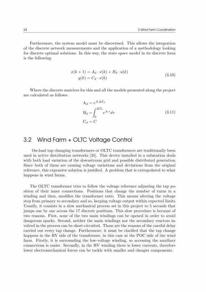
Furthermore, the system model must be discretised. This allows the integrationof the discrete network measurements and the application of a methodology lookingfor discrete optimal solutions. In this way, the state space model in its discrete formis the following:
x(k + 1) = Ad · x(k) + Bd · u(k)y(k) = Cd · x(k)
(3.10)
Where the discrete matrices for this and all the models presented along the projectare calculated as follows:
Ad = eA·∆Td
Bd =∫ ∆Td
0eA·τ dτ
Cd = C
(3.11)
3.2 Wind Farm + OLTC Voltage ControlOn-load tap changing transformers or OLTC transformers are traditionally been
used in active distribution networks [35]. This device installed in a substation dealswith both load variation of the downstream grid and possible distributed generation.Since both of them are causing voltage variations and deviations from the originalreference, this expensive solution is justified. A problem that is extrapolated to whathappens in wind farms.
The OLTC transformer tries to follow the voltage reference adjusting the tap po-sition of their inner connections. Positions that change the number of turns in awinding and then, modifies the transformer ratio. This means altering the voltagestep from primary to secondary and so, keeping voltage output within expected limits.Usually, it consists in a slow mechanical process set in this project to 5 seconds thatjumps one by one across the 17 discrete positions. This slow procedure is because oftwo reasons. First, none of the two main windings can be opened in order to avoiddangerous sparks. Second, neither the main windings nor the secondary reactors in-volved in the process can be short-circuited. Those are the reasons of the careful delaycarried out every tap change. Furthermore, it must be clarified that the tap changehappens in the HV side of the transformer, in this case at the POC side of the windfarm. Firstly, it is surrounding the low-voltage winding, so accessing the auxiliaryconnections is easier. Secondly, in the HV winding there is lower currents, thereforelower electromechanical forces can be tackle with smaller and cheaper components.

3.2 Wind Farm + OLTC Voltage Control 25
3.2.1 OptimisationIn this second strategy, the wind farm voltage control is coordinated with the
OLTC transformer. Still, the procedure for the optimisation problem within the MPCis the same as in Section 3.1.1. It consists of two modes and four elements as before,but the first element (controlled variables) adds up a new measurement of the currenttap position: ntap.
Secondly, the decision variables integrate a new parameter: ∆ntap. It is the tapposition increment of the main transformer (OLTC) of the wind farm. Accordingto the discrete characteristic of the machine, the variable is declared as an integernumber.
Thirdly, the objective function remains unchanged, so equal to Equation (3.1).However, its three components integrate new elements related to tap changes. Re-garding the prediction horizon Tp, it is now 10 seconds in order to hold the slowprocess of the tap transformer. Yet, Tc and ∆Tp are the same value as for thefirst strategy to integrate the fast changes of WTGs. The three components of theobjective function are the following:
∆V preP OC(k) = VP OC(k) − V ref
P OC + ∂|VP OC |∂QW T
· ∆QW T (k) (3.12)
∆V preMV (k) = VMV (k) − V ref
MV + ∂|VMV |∂QW T
· ∆QW T (k) + ∆|VMV |∆ntap
· ∆ntap(k) (3.13)
∆V preW T (k) = VW T (k) − V ref
W T + ∂|VW T |∂QW T
· ∆QW T (k) + ∆|VW T |∆ntap
· ∆ntap(k) (3.14)
As it can be seen, Equation (3.12) is equal to Equation (3.2). It is because an elec-trical coupling is considered between the POC bus and the main bus of the externalnetwork. That means that the effect of a tap change is neglected in the HV side of thetransformer. On the other side, Equation (3.13) and (3.14) include the new decisionvariable ∆ntap. Then, the effect of a tap change is indeed considerable for the restof buses, assuming the POC bus as the reference k. Its multiplier corresponds to thevoltage magnitude sensitivity to each tap step.
Fourthly, the same constraints (3.5) and (3.6) are considered. Moreover, theoperational limits of the OLTC are included in. First, it only can change positionsone by one. Second, the configuration range has 17 positions. These constraints areimplemented as follows:
−1 ≤∆ntap(k) ≤1−8 ≤ntap(k) ≤8 (3.15)

26 3 Wind Farm Coordination
Finally, a conditional and temporal limit (3.16) is created as security delay. Inspite of the operational delay, an extra second limit ensures that the transformer ismechanically stabilised after a tap step and there is no risk of too many electricalcontacts at the same time.
∆ntap(k) =
∆ntap(k), ift0∑
k=t0−5
∆ntap(k) = 0
0, otherwise(3.16)
3.2.2 State Space Model
After the presentation of optimisation changes related to this second strategy,the modifications in the modelling part are going to be explained in this section.The system state space model keeps being the same as presented in Equation (3.7).However, its elements are modified in order to integrate the new decision variable∆ntap. Firstly, the variables of the system are the following:
x = [∆QW T1 , ..., ∆QW TNW, ∆ntap]T
u = [∆QrefW T1
, ..., ∆QrefW TNW
, ∆nreftap ]T
y = [∆QW T1 , ..., ∆QW TNW, ∆ntap]T
Where the new decision variable related to the OLTC of the output variable arrayy can be identified in Equations (3.13) and (3.14). Therefore, integrating also theinput variable u and its tap reference into the minimisation process.
Next, the associating matrices holding the dynamics of the system elements arepresented. Regarding WTGs, the model and AW T , BW T , CW T matrices remainthe same. On the other hand, the OLTC behaviour is introduced here. In theprevious research work, the OLTC was automatically controlled by its automaticvoltage regulator (AVR) as it is shown in Figure 3.2. However, now it is controlledby the MPC. Then, a tap position change in reference ∆nref
tap is the input of thecontrol system instead of voltage reference desired. Eventually, only the time-delayis modelled from the AVR reference.

3.3 Wind Farm + VSC-HVDC Voltage Control 27
Figure 3.2: AVR control of a OLTC transformer [36]
Therefore, the mechanical delay of a change in internal connections is modelledas Ttap. What is considered as 5 seconds in this case. The state space model ofthe transformer is presented in Equation (3.17) as a dynamic model and in Equation(3.18) as an already discrete model due to its simplicity.
∆ ˙ntap = AOLT C · ∆ntap + BOLT C · ∆nreftap (3.17)
∆ntap(k) = ∆nreftap (k − Ttap) (3.18)
3.3 Wind Farm + VSC-HVDC Voltage ControlHVDC technology is already widely spread since the first submarine cable was
installed in Sweden in 1954. Some of its advantages are presented in [37]: lower in-vestment cost from 50 km or longer cables, lower power losses, there is not reactivepower generation such that in long AC cables, it can connect different synchronoussystems and it allows controlling power parameters. However, it is getting more at-tractive because of two reasons. First, many offshore wind farms are being plannedand HVDC is a solution for transmitting bulk power across long-distance submarinecables. Second, there are proposals of a DC-supergrids for European-level intercon-nection [38].
According to those challenges, the voltage sourced converter (VSC) technologywas developed. Firstly, it offers fast and full controllability of the converter terminal,even AC active and reactive power independently. Secondly, it allows a multi-terminal

28 3 Wind Farm Coordination
(MT) solution. Its main differences with the traditional HVDC-converter methodol-ogy [39] are: the use of bidirectional controlled thyristor and an inductive reactorbetween the converter terminal and the network. Besides, it still integrates the usualfilters and DC capacitors. Furthermore, some more advantages are simple control,few harmonic generation, adjustable power factor and black up capability.
In spite of the wide use of the VSC technology, most of the literature is focusedon the DC-voltage control for MT-grid control. For this reason and with a assumedDC-supergrid working as a slack bus and taking care of the DC-voltage, this projectaims at controlling the AC-terminal of the VSC converter what would bring somebenefits for the wind farm side terminal despite of the DC-link.
3.3.1 OptimisationAlong this third strategy, the coordinated device is the VSC of the wind farm
side. As it is explained for the OLTC, the optimisation problem follows the structurepresented in Section 3.1.1. Again, the controlled variables are the first part of theproblem and they remain the same.
Secondly, a new decision variable comes up as ∆Vc. It states the voltage mag-nitude increment of the voltage-sourced converter (VSC) on the AC-terminal of thewind farm side. This new variable is added up to the ∆QW T array, but the ∆ntap isnot considered any more.
Thirdly, the same objective function is defined according to Equation (3.1). Theprediction horizon has the same value as in the first strategy, Tp = 5seconds. Sincethe VSC dynamics make fast effects, no more time is considered. Each of the threeelements of the objective functions are presented here:
∆V preP OC(k) = VP OC(k) − V ref
P OC + ∂|VP OC |∂QW T
· ∆QW T (k) + ∂|VP OC |∂Vc
· ∆Vc(k)
(3.19)
∆V preMV (k) = VMV (k) − V ref
MV + ∂|VMV |∂QW T
· ∆QW T (k) + ∂|VMV |∂Vc
· ∆Vc(k) (3.20)
∆V preW T (k) = VW T (k) − V ref
W T + ∂|VW T |∂QW T
· ∆QW T (k) + ∂|VW T |∂Vc
· ∆Vc(k) (3.21)
Unlike Equation (3.12), Equation (3.19) takes into account the new decision vari-able. That is because the HVDC link decouples the wind farm from the main network,so every change in the VSC terminal makes a direct effect in every bus. Therefore,

3.3 Wind Farm + VSC-HVDC Voltage Control 29
Equations (3.19), (3.20) and (3.21) integrates the influence of ∆Vc. Its multiplier cor-responds to the voltage magnitude sensitivity regards to the mentioned AC terminal,which is explained in Section 2.4 and its reference k bus corresponds to the POC bus.
Fourthly, constraints (3.5) and (3.6) are included again in this problem. At thesame time, the AC-terminal of the VSC of the wind farm side is limited by theconstraint which includes the voltage threshold at the POC bus.
3.3.2 State Space ModelRegarding this third strategy and the installation of the VSC-HVDC, it also
makes some modifications in the modelling part. Based on the same state spacemodel presented in Equation (3.7), the variables of the system must now include inthe decision variable ∆Vc of the optimisation. The output variables array y can befound in Equations (3.19), (3.20) and (3.21) while all the variables are the following:
x = [∆QW T1 , ..., ∆QW TNW, ∆ud_ref
s , ∆uds , ∆ud
int, ∆idP I ]T
u = [∆QrefW T1
, ..., ∆QrefW TNW
, ∆V refs ]T
y = [∆QW T1 , ..., ∆QW TNW, ∆Vc]T
Where ∆Vc and ∆V refs are voltage magnitude increments at the VSC-terminal
of the wind farm side and at the POC bus. It means between the two points ofmeasurement are some losses modelled such as filters, phase reactor and internalelements. Losses represented by Cf in the following equations. On the other hand,the new state variables ∆ud_ref
s , ∆uds , ∆ud
int, ∆idP I are respectively voltage magnitude
reference increment from the MPC, voltage magnitude measurement increment, aninternal control voltage magnitude increment and current increment from the PIcontroller of the inner loop. All of them are referred to the parameter d, whichstates the d-axis from the dq-frame. Taking into account the following assumption:Vs =
√(ud
s)2 + (uqs)2 ≈ ud
s .Although WTGs elements are the same as presented in Sections 3.1.2 and 3.2.2,
the VSC parameters must be explained with a control scheme. While a simplificationsuggested by [28] is shown in Figure 3.3, its parameters and the relationship withabove variables are stated in the following transfer functions. First, the Delay blockcorresponds to a Td first-order delay function in (3.22). Second, the uACOuterLoopcorresponds to the PI controller (second term) within (3.25), with ko_p as the pro-portional gain and ko_i as the integral gain. Third, the idqInnerLoop is simplifiedas a Tinr simplified time constant of the inner control loop within (3.25)(first term).Fourth, the PhysicalF ilterModel regards to the Cf capacitor filter in (3.23).
∆ud_refs = 1
1 + s · Td· ∆V ref
s (3.22)
∆uds = − 1
s · Cf· ∆id
P I (3.23)

30 3 Wind Farm Coordination
Figure 3.3: VSC Control Scheme
∆udint = ∆ud_ref
s − ∆uds
s(3.24)
∆idP I = − 1
1 + s · Tinr·(
ko_p + ko_i
s
)(∆ud_ref
s − ∆udss) (3.25)
Where
∆V refs = V ref
s − Vs(t0),∆ud_ref
s = ud_refs − us(t0),
∆uds = ud
s − us(t0),
and, all the values of these variables are shown in the following Table 3.1.
VSC ParametersParameter ValueCf 10−6 FTd 0.1 secTinr 0.005 secko_p 0.1ko_i 10
Table 3.1: VSC Parameters
To sum up, the VSC dynamic state space model shows like the following equation:
˙xV SC = AV SC · xV SC + BV SC · uV SC
yV SC = CV SC · xV SC
(3.26)
Where xV SC = [∆ud_refs , ∆ud
s , ∆udint, ∆id
P I ]′ , uV SC = [∆V refs ] and, yV SC =
[∆Vc]. Eventually, the associating matrices of the device are the following:

3.4 Power Factory 31
AV SC =
− 1Td
0 0 0
0 0 0 1Cf
1 −1 0 0
−ko_p
Tinr−ko_p
Tinr−ko_i
Tinr− 1
Tinr
,
BV SC =
1Td000
,
CV SC =(∂|Vs|
∂|Vc|
)−1 [0, −1, 0, 0
],
3.4 Power Factory
3.4.1 Wind Farm Voltage ControlAs it is introduced at the beginning of this chapter, Power Factory is the tool for
implementing the physical network and controllers. This project is developed overthe so-called Nordic32 power system which can be seen in Figure 3.4. It is suggestedby the IEEE as a benchmark for voltage stability and dynamic studies. Specifically,the voltage control analysis addresses a new offshore wind farm connected to bus 1042of the Central grid.
A more accurate description of the wind farm topology is shown in Figure 3.5.There are 20 x 5 MW type-4 WTGs and an OLTC transformer, that for this firststrategy it disables the AVR controller hence it is a common transformer with fixedtap position. In addition, the VSC-HVDC system is also disabled for this strategy.
Next, it is going to be explained the most important part of the Power Factorywork. This is the voltage controller. It is implemented as an ElmV ol slot within aframe. This frame provides a series of slots such as measurement of voltage buses,measurement of WTG power supply and the WTG machine indeed receiving refer-ences from the MPC voltage controller. Thus, working as an integrating interface formeasurements, signals and devices of the topology previously mentioned.
Further details of the voltage controller are shown in Figure 3.6. There, the re-lationship between the controller and its signals can be seen on the left side. First,the measurements of voltage magnitude VW T and voltage phase θW T for each of the20 WTGs. The same parameters are measured for the three main buses of the wind

32 3 Wind Farm Coordination
Figure 3.4: Nordic32 Power System [40]: Single-Line Diagram
farm: external bus 1042 Vext, point of connection VP OC and medium-voltage bus VMV .Moreover, current active and reactive power of each of the WTGs is also considered asan input: PW T and QW T . Eventually, a variable with simulation time is calculatedand communicated for the right interaction between the two softwares. On the otherhand, the voltage controller output corresponds to the output of the MPC. In thisstrategy, this is an array with the reactive power reference Qref
W T of each of the WTGs.
Furthermore, its communication with Matlab is presented on the right side ofFigure 3.6. There, a routine is run representing the whole MPC. In this case, eachof the stages are organised as the process is developed. In conclusion, the MatlabMPC works as an embedded function within the voltage controller slot for the restof elements of Power Factory frame.

3.4 Power Factory 33
Figure 3.5: Wind Farm Network: Single-Line Diagram
Figure 3.6: Voltage Controller Scheme
Finally, it is worth noting a WTG model implemented in Power Factory. A simpli-fied example is shown in Figure 3.7. First, a slot represents the time-delay accordingto the transfer function explained in Equation (3.8). Second, the electrical machineis modelled as a variable load. Thus, an inversion of signs is needed for the outputparameters. Regarding the input signals of the WTG, firstly Qref
W T comes from theMatlab MPC algorithm and provides the reference VAR output of the machine. Sec-ondly, VW T and θW T are the measurements from the network buses. Thirdly, P av
wind
states the available power in the wind limiting the electrical maximum output of thegenerator. These parameters will determine the operational behaviour of the windturbine, hence providing the actual active P ext
W T and reactive QextW T power supply.

34 3 Wind Farm Coordination
Figure 3.7: WTG Scheme
3.4.2 Wind Farm + OLTC Voltage ControlBased on the same system topology, the second voltage control analysis is ad-
dressed. Still, the OLTC AVR and the VSC-HVDC are out of service within thewind farm. Otherwise, the OLTC is now controlled by the MPC algorithm. Indeed,its optimal tap position nopt
tap is updated according to the decision variable ∆ntap inEquations (3.13) and (3.14). A schematic representation is shown in Figure 3.8 layingdown in the following expression: nopt
tap = ntap + ∆nreftap .
Figure 3.8: OLTC Scheme
Consequently, the voltage controller is updating the current measured tap positionntap with the incremental tap step decided in the optimisation part of the MatlabMPC function. This current measurement comes from the OLTC slot which statesthe electrical machine displayed as an ElmTr2 element. On the other hand, moresignals can be found in the layout. First, the dotted input represents all the inputmeasurements as they are in Figure 3.6. Second, the output reference for WTGs,which also remains the same. Third, the tap_history loop. This signal consists of amemory variable for next MPC iteration. It is an array which handles the last fivetap position increments decided by the minimisation process. Thus, it carries outtwo functions. Firstly, the reminder checks out the constraint (3.16). Secondly, itperforms the discrete machine model of Equation (3.18).

3.4 Power Factory 35
3.4.3 Wind Farm + VSC Voltage Control
Following the same procedure, the third voltage control is tested again in theNordic32 system. However, the wind farm topology is now modified. The AC lineis swithced off and the DC system is operational in this case. Regarding the OLTC,both the AVR and the MPC control for this device are disabled hence a fixed tapposition is set. However, the MPC takes over the wind farm VSC-terminal and WTGsas well. In this case, the voltage controller scheme corresponds to Figure 3.9. Thereare two output signals now. First, Qref
W T and second, a new reference for the voltagemagnitude of the VSC terminal V ref
s . This voltage reference comes from the followingequation: V ref
s = VP OC +∆V refs . Where the former term is the current measurement
and the latter comes from the MPC optimisation solution. It must be reminded that∆V ref
s is related to ∆Vc through the state space model in Section 3.3.2. Being thislast variable, the one which appears in the objective function terms from Equation(3.19) to (3.21).
Figure 3.9: Wind Farm VSC Scheme
Regarding the rest of members in Figure 3.9, there are three new slots. First, thePhase Locked Loop (PLL) supplies reference signals cosphi and sinphi to the con-verter based on the frequency and phase of its input. These parameters are measuredat Bus1042 − CentralNetwork with a synchronised oscillator. Second, the convertercontroller. It is receiving the reference V ref
s and the measurement of the currentvoltage at the VSC terminal. Then, providing the modulation indexes P d
m and P dm,
that control the behaviour of the real converter. The former one comes from the con-trol scheme showed in Figure 3.3 to control the AC-voltage. The latter one is set tozero, as its controlled parameters (active power or DC-voltage)[41] are not of interest.Third, the slot V SCConverter states the real power-electronics machine modelled inthe wind farm network. A 300-MVA device rated at 130kVAC and 225kVDC workingin a VAC −θ control mode. On the other hand, the terminal connected to the externalnetwork works in VDC − Q mode.

36 3 Wind Farm Coordination
3.5 Results and DiscussionAn assessment of the voltage controllers is carried out in this section. Each of
them is tested through a dynamic or root-mean-square (RMS) simulation in PowerFactory. This test consists of a 100-second study in which a WTG power outputvariation is implemented. Each of the machines is working around their 4-MW ofactive power supply. Therefore, power oscillations from 74 to 78 MW can be seenas a WF output in Figure 3.10. The input data states available power in the wind,which was generated in SimWindFarm integrating wind field models of turbulancesand wake effects. Although a bigger variation in power could have been studied,this specific range was chosen due to the limited reactive power supply of WTGs.VAR contribution which is challenged for being close to their maximum active poweroutput, as it is shown in the capacity curve of a WTG in Figure 3.1.
Figure 3.10: Wind Farm Active Power Output
3.5.1 Wind Farm Voltage ControlAiming at a voltage profile improvement along the buses of the WF, this first
strategy faces this main objective through the VAR supply of the WTGs. After asimulation, it can be highlighted that none of the nodes goes beyond their respectiveboundaries. That means that the voltage controller is all the time in PreventiveModeand hence, only the voltage magnitude at the POC bus is optimised every iteration.This allows a comparison of the results of each strategy focusing on the voltage profileat this bus: VP OC , which is illustrated in the upper part of Figure 3.11. Furthermore,the voltage magnitude at the MV bus VMV is going to be analysed too and is shownin the lower part. It might state the behaviour of further WTG buses due to its directrelationship as a power collector.
It is clearly appreciable the improvement provided by the MPC optimisation.Along the simulation time in Figure 3.11 it minimises the voltage magnitude de-

3.5 Results and Discussion 37
Figure 3.11: WFVC: Voltage Magnitude at POC and MV buses
viation from the bold-dashed reference at V refP OC = 1p.u.. Then, the absolute voltage
error is reduced from et5P OC = 0.006p.u. to et100
P OC = 0.0003p.u. at the last iteration.An interesting detail of the MPC can be pointed out. The control modelling parttakes into account the dynamics of the generators and their time-delay response.Hence, avoiding an overshoot of the voltage wave after the control action takes overthe VAR supply at tsim = 5s. However, the MV bus voltage profile does not showsuch good improvement. Even more, its error increses from e5
MV = 0.0051p.u. toe100
MV = 0.0128p.u.. An error did not address by the MPC, since it is not included inthe objective function of this operational mode. Nonetheless, it is reminded that isnot go over its threshold set to V th
MV = 0.03p.u..
Finally, Figure 3.12 illustrate the behaviour of some representative WTGs. Theyare: WT1, WT7 and WT16 which are chosen for being the first and last generatorsof the longest feeder and, for belonging to the fourth feeder in the last case. Therein,the upper part shows a lower average deviation from the voltage reference. Evenbeing almost zero for some of the machines. Thus, it states how the drop of voltagewhich was considered as a drawback for the MV bus brings an overall advantage forthe WTG buses. Eventually, the reactive power response of those WTGs can be seenin the lower part. Their negative or absorbing behaviour help the machine nodes tofall their respective voltages. This approach represents until 1.406MV Ar of inductivereactive power from the load perspective in the WT1 case.

38 3 Wind Farm Coordination
Figure 3.12: WFVC: Voltage Magnitude and Reactive Power of WTGs
3.5.2 Wind Farm + OLTC Voltage Control
Secondly, it is going to be explained how the control of an OLTC transformerupgrades the voltage evolution along the simulation. Again, the PreventiveModeprevails along the simulation and so, the VP OC is the main target to care about. Thismagnitude and VMV are illustrated in Figure 3.13. Since in the previous simulationthe MV boundary was not even close, this time and on V th
MV = 0.01p.u.. Hence,tighten constraints will challenge more the system. As it can be noticed, the VP OC
variable performs exactly the same as in the case without OLTC. This is becauseof two reasons. First, the POC bus is coupled to the external network. Therefore,small changes within the WTGs contribution does not make a considerable influence.Second, the same coupling makes an OLTC tap change to modify only the voltagesdownwards itself. Therefore, the rest of WF buses suffers a modification. Regardingthe tap change, this is a control action from the MPC in order to avoid the boundarynow set at 0.99 p.u.. Firstly, it means a considerable improvement for the MV bussince it reduces the voltage deviation. The absolute error at t = 100s reaches eOLT C
MV =0.0001p.u. regarding an initial eInit
MV = 0.0051p.u. and eW F V CMV = 0.0128p.u. for the
strategy WFV C.

3.5 Results and Discussion 39
Figure 3.13: WF+OLTC VC: Voltage Magnitudes
Secondly, another modification is generated in the rest of WTG buses. The voltagestep moves away all the magnitudes from their respective reference. This makes aworse situation for all the WTG nodes. This voltage change in some representativenodes can be seen in Figure 3.14. Moreover, the reactive power change from theWFV C strategy is shown too. There, it can be observed how the voltage step forcedby the system pulls also the reactive power. What it is counteracted afterwards bythe MPC control.
Further detail of the tap change is illustrated in Figure 3.15. The decision variable∆Ntap from the MPC optimisation is shown there. Reminding that this variable mustbe discrete according to the transformer characteristics, a filter must be applied tothis decision variable. Consequently, only a tap change is carried out over a certainthreshold N th
tap = 0.75. In the detail section within the figure is shown how a tap-downstep (solid line) is applied at t = 41s, exactly Ttap = 5s after the decision variableovertakes the red boundary.

40 3 Wind Farm Coordination
Figure 3.14: WTGs: Voltage Magnitude & Reactive Power
Figure 3.15: WF+OLTC VC: OLTC Tap Change Detail

3.5 Results and Discussion 41
3.5.3 Wind Farm + VSC Voltage Control
Thirdly, the controllability of the WF-VSC terminal is studied in this simula-tion. The AC voltage magnitude control provides further improvements which areillustrated in Figure 3.16. Therein, the VP OC and VMV are shown and their absoluteerrors must be analysed for further comparison with the other strategies. Firstly,the error at t = 100s is now eV SC
P OC = 0.0003p.u. while it was eInitP OC = 0.006p.u. and
eW F V CP OC = eOLT C
P OC = 0.0003p.u.. Secondly, for the other bus is eV SCMV = 0.0009p.u.
while it was eInitMV = 0.0051p.u., eW F V C
MV = 0.0128p.u. and eOLT CMV = 0.0001p.u.. Thus,
getting with the VSC the same steady deviation in the POC bus and a worse steadyvalue in the MV, according to the OLTC results.
Further detail of the VSC behaviour is illustrated in Figure 3.17. First, it appearsthe active power output of the WF which is injected into the converter. It is directlyrelated to the V DC
V SC variable of the HVDC-link, which is shown in the second part ofthe illustration. Therein, it is compared to V AC
V SC = VP OC and to VMV . Furthermore,VP OC is controlled by the converter and hence, it is directly influencing the reactivepower supply by the converter in the third part of the illustration.
Figure 3.16: WF+VSC VC: Voltage Magnitude at POC and MV buses

42 3 Wind Farm Coordination
Figure 3.17: WF+VSC VC: VSC WF-Terminal Outputs
3.5.4 Discussion
Summing up, the three voltage controllers based on MPC enhance the voltageprofile at the POC. Consequently, a good performance of the MPC can be acknowl-edged, since that node was mainly covered by the objective function. Moreover, whentwo of those, the OLTC and the VSC, manage a decision variable the MV bus alsogets an enhancement. These two facts are summarised in Figure 3.18.
On the other hand, the rest of nodes in the WF do not follow the same accuracyto the reference. Still, all the magnitudes are within safe limits. Besides, the threestrategies get an improvement from the initial simulation without voltage control.Regarding these WTG buses, the best performance is achieved while controlling onlythe WTG VAR response (WT MPC). An overall analysis is illustrated in Figure 3.19through the maximum and minimum voltage magnitude level for each controller.Therein, the WFVC or WF MPC gets the reference magnitude between its two WTGvoltage levels. Therefore, ensuring all the other voltages in between and hence, theaverage range of voltages is closer to V ref
W T = 1p.u..
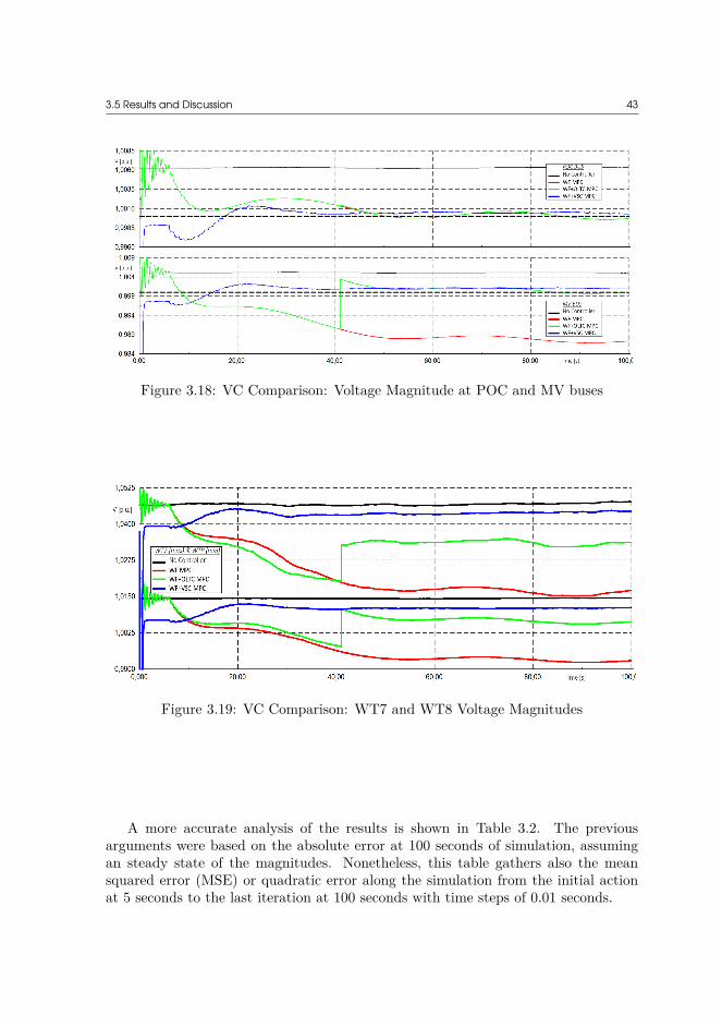
3.5 Results and Discussion 43
Figure 3.18: VC Comparison: Voltage Magnitude at POC and MV buses
Figure 3.19: VC Comparison: WT7 and WT8 Voltage Magnitudes
A more accurate analysis of the results is shown in Table 3.2. The previousarguments were based on the absolute error at 100 seconds of simulation, assumingan steady state of the magnitudes. Nonetheless, this table gathers also the meansquared error (MSE) or quadratic error along the simulation from the initial actionat 5 seconds to the last iteration at 100 seconds with time steps of 0.01 seconds.

44 3 Wind Farm Coordination
VC Error ComparisonVoltage Absolute POC Error Absolute MV Error MSE POC ErrorControl et100
P OC (p.u.) et100MV (p.u.) ε2
P OC (p.u.)No Contr. 0.0060 0.0051 3.9542 × 10⁻⁵
WF 0.0003 0.0128 2.1790 × 10⁻⁶
WF+OLTC 0.0003 0.0001 2.1845 × 10⁻⁶
WF+VSC 0.0003 0.0009 8.9076 × 10⁻⁷
Table 3.2: Voltage Controller Error Comparison
Consequently, the following comments can conclude this study. According to theabsolute error at the POC, any of the controllers bring an excellent performance.Then, the absolute error at the MV bus might be a decision aspect since the bestbehaviour is found in the WF+OLTC voltage control strategy. Otherwise, the MSEsuggests that the lower error and hence, the best controller is the WF+VSC. Toconclude, the final decision is accepting the WF+VSC voltage control strategy as thebest one and so, implementing it in further studies. This decision is made according tofour reasons. First, the MSE is considered more important since it takes into accountthe whole simulation time. It means a faster error minimisation. Second, the MSEstates the objective function of the MPC optimisation. Thus, it respects strictly thetarget set at the beginning of the study. Third, the difference between the two laststrategies in regards to the absolute error at the MV bus is considered as acceptable.Fourth, the VSC-HVDC technology is more attractive for future multiterminal DCnetworks from a subjective point of view.

CHAPTER 4Network Coordination
4.1 Wind Farm + External OLTC Voltage ControlOnce different technologies have been tested within the wind farm, it is time to
try to coordinate them when they are installed outside the wind farm, i.e. in the mainnetwork. In this way, addressing the second challenge introduced in the objectives.Then, aiming at getting some voltage benefits also in external buses of the system.
Based on the comparison analysis carried out in previous chapter, the windfarm topology is set through the VSC-HVDC technology connected to Bus1042 −CentralNetwork. Meanwhile, an OLTC transformer in CentralNetwork is going tobe controlled too. Therefore, coordinating both technologies for two purposes. First,keeping an optimal voltage level within the offshore grid. Second, improving thevoltage profile of a close area to which the wind farm is connected.
Figure 4.1: External Distribution Network: Single-Line Diagram
The OLTC installation is based on an approach to active management of gridswith distributed energy resources (DER). Voltage variability would be produced dueto the weather changing conditions affecting generation and energy storage systems.Then, this kind of network is assumed as connected to Bus1042 − CentralNetwork,as it can be seen in Figure 4.1. Modelling variability issues is carried out by a variableload along the time, following a consumption pattern from household demands. Asvoltage control is the target, a major role is given to the reactive power demand forcreating voltage variations. While a static load is set as 50 MW and 50 MVAr, thevariable part of this load is following a profile with 70 MVar of maximum capacity.This profile can be seen in Figure 4.2 once is connected at 40 seconds.
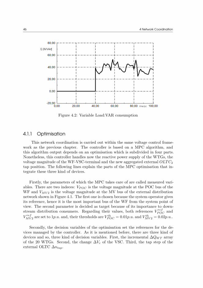
46 4 Network Coordination
Figure 4.2: Variable Load:VAR consumption
4.1.1 OptimisationThis network coordination is carried out within the same voltage control frame-
work as the previous chapter. The controller is based on a MPC algorithm, andthis algorithm output depends on an optimisation which is subdivided in four parts.Nonetheless, this controller handles now the reactive power supply of the WTGs, thevoltage magnitude of the WF-VSC-terminal and the new aggregated external OLTC2tap position. The following lines explain the parts of the MPC optimisation that in-tegrate these three kind of devices.
Firstly, the parameters of which the MPC takes care of are called measured vari-ables. There are two indeces: VP OC is the voltage magnitude at the POC bus of theWF and VMV 2 is the voltage magnitude at the MV bus of the external distributionnetwork shown in Figure 4.1. The first one is chosen because the system operator givesits reference, hence it is the most important bus of the WF from the system point ofview. The second parameter is decided as target because of its importance to down-stream distribution consumers. Regarding their values, both references V ref
P OC andV ref
MV 2 are set to 1p.u. and, their thresholds are V thP OC = 0.01p.u. and V th
MV 2 = 0.02p.u..
Secondly, the decision variables of the optimisation set the references for the de-vices managed by the controller. As it is mentioned before, there are three kind ofdevices and so, three kind of decision variables. First, the incremental ∆QW T arrayof the 20 WTGs. Second, the change ∆Vc of the VSC. Third, the tap step of theexternal OLTC ∆ntap.

4.1 Wind Farm + External OLTC Voltage Control 47
Thirdly, the objection function (4.1) tries to minimise the voltage error of themeasured variables to their respective references. The same function is applied as inthe previous optimisation sections. However, there are only two predicted error terms(4.2) and (4.3) within it, related to the two measured variable presented above. Thelong-term deviation is considered with Np predicted steps coming from a predictionhorizon Tp = 10seconds and a prediction period ∆Tp = 0.5seconds.
min∆QW T ,∆Vc,∆ntap
Np∑k=1
(∥∆V preP OC(k)∥2 + ∥∆V pre
MV 2(k)∥2) (4.1)
∆V preP OC(k) = VP OC(k) − V ref
P OC + ∂|VP OC |∂QW T
· ∆QW T (k) + ∂|VP OC |∂Vc
· ∆Vc(k) (4.2)
∆V preMV 2(k) = VMV 2(k) − V ref
MV 2 + ∆|VMV 2|∆ntap
· ∆ntap(k) (4.3)
Where all the terms have been introduced above and the partial derivatives cor-responds to the sensitivity coefficients explained in Section 2.4. Respectively, thesensitivity to VAR response is calculate in Equation (2.8), the sensitivity to VSC-voltage change in Equation (2.14) and the sensitivity to tap changes in Equation(2.15). Nevertheless, it must be highlighted their reference k bus for the calculation.In spite of the fact that for the whole project and for the coefficients in (4.2) this busis the POC bus of the WF, the new external distribution network make them change.Thus, the new network Ybus2 must be considered in (4.3). Its new k reference bus isthe bus HV-side of the new OLTC2.
Fourth, the problem is constrained by the physical limits of network devices. Tosum up, the following equations gather all ones already mentioned. Where WTGreactive power limits are in (4.4) and the transformer operational limits are in (4.5)to (4.7).
QminW Ti
(k) ≤ QW Ti(k) ≤ Qmax
W Ti(k)
∀i ∈ [1, 20], k ∈ [1, Np](4.4)
−1 ≤∆ntap(k) ≤1 (4.5)
−8 ≤ntap(k) ≤8(4.6)
∆ntap(k) =
∆ntap(k), ift0∑
k=t0−5
∆ntap(k) = 0
0, otherwise(4.7)

48 4 Network Coordination
4.1.2 State Space ModelThe second part of the MPC algorithm consists of defining the network dynamics
in order to integrate them into the previous optimisation. The dynamic behaviourof each of the elements controlled by the MPC has already been introduced in theprevious chapter. However, their equations are summarised below for a good com-prehension. Further details are already explained in the StateSpaceModel Sectionsbefore. First, the system continuous state space model is the following:
x = A · x + B · u
y = C · x(4.8)
Where their variables integrate now the three kind of devices in charge of thevoltage control. Thus, appearing as decision variables in Equations (4.2) and (4.3).They are described as follows:
x = [∆QW T1 , ..., ∆QW TNW, ∆ntap, ∆ud_ref
s , ∆uds , ∆ud
int, ∆idP I ]T
u = [∆QrefW T1
, ..., ∆QrefW TNW
, ∆nreftap , ∆V ref
s ]T
y = [∆QW T1 , ..., ∆QW TNW, ∆ntap, ∆Vc]T
Later on, the associating matrices of the system A, B and C are described individ-ually for each of machine. First, the WTG dynamics are the following: Ai
W T = −1TW T
and BiW T = 1
TW T. Then, developing them for the machines of the whole system are:
AW T = diag(A1W T , ..., ANW
W T )BW T = diag(B1
W T , ..., BNW
W T )CW T = diag(11, ..., 1NW
)
Second, the VSC behaviour is gathered in matrices AV SC , BV SC and CV SC inPage 31.
Third, the OLTC2 is represented by the following discrete equation due to itssimplicity. Consequently, substituing the general continuous model (4.8), which willbe discretised afterwards for the optimisation calculation.
∆ntap(k) = ∆nreftap (k − Ttap) (4.9)
4.2 Power FactoryThe network topology design is carried out in PowerFactory as it is stated before.
The whole system Nordic32 and the controlled wind farm are illustrated in Figures 3.4and 3.5. The new distribution grid with the variable load is design according toFigure 4.1. Then, it is connected to Bus1042 − CentralNetwork. Next, the voltagecontrol explained in Section 4.1 is illustrated on the scheme in Figure 4.3. Therein, the

4.3 Results and Discussion 49
voltage controller included in a PowerFactory frame manages the WTGs, the externalOLTC2 and the WF-VSC. Consequently, the coordinated strategy is implemented.
Figure 4.3: Voltage Control Scheme
4.3 Results and DiscussionThe last coordinated voltage controller is going to be tested following the same
procedure as for the WF alone. This is through a 100-second RMS simulation inPower Factory. An active power variation challenges the performance of the controlstrategy for assessment. This power variation is the same as introduced before inFigure 3.10. Moreover, the consumption load also implies an impact at the Bus1042in comparison to the case without variable load. This considerable effect in thereference bus is illustrated in Figure 4.4.
Figure 4.4: Voltage Impact in Bus 1042 due to Variable Load
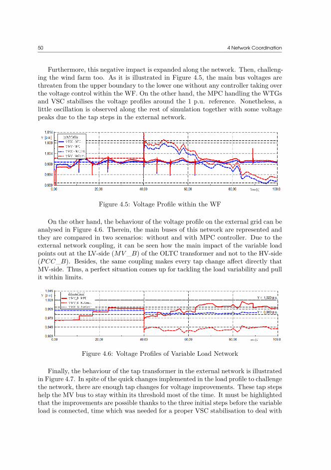
50 4 Network Coordination
Furthermore, this negative impact is expanded along the network. Then, challeng-ing the wind farm too. As it is illustrated in Figure 4.5, the main bus voltages arethreaten from the upper boundary to the lower one without any controller taking overthe voltage control within the WF. On the other hand, the MPC handling the WTGsand VSC stabilises the voltage profiles around the 1 p.u. reference. Nonetheless, alittle oscillation is observed along the rest of simulation together with some voltagepeaks due to the tap steps in the external network.
Figure 4.5: Voltage Profile within the WF
On the other hand, the behaviour of the voltage profile on the external grid can beanalysed in Figure 4.6. Therein, the main buses of this network are represented andthey are compared in two scenarios: without and with MPC controller. Due to theexternal network coupling, it can be seen how the main impact of the variable loadpoints out at the LV-side (MV _B) of the OLTC transformer and not to the HV-side(PCC_B). Besides, the same coupling makes every tap change affect directly thatMV-side. Thus, a perfect situation comes up for tackling the load variability and pullit within limits.
Figure 4.6: Voltage Profiles of Variable Load Network
Finally, the behaviour of the tap transformer in the external network is illustratedin Figure 4.7. In spite of the quick changes implemented in the load profile to challengethe network, there are enough tap changes for voltage improvements. These tap stepshelp the MV bus to stay within its threshold most of the time. It must be highlightedthat the improvements are possible thanks to the three initial steps before the variableload is connected, time which was needed for a proper VSC stabilisation to deal with

4.3 Results and Discussion 51
Figure 4.7: Tap Position of OLTC2
the fast changes. However, the slow dynamics of this device are present. Then,a perfect behaviour can not be achieved. Although an ideal voltage profile is notachieved, the improvements of handling the OLTC are shown in Table 4.1. In thiscase, the absolute error is dismissed due to the fast and constant changes of theVAR load profile. Then, the mean squared error brings a more accurate idea of theperformance in comparison to the quadratic error objective function. This MSE iscalculated from t = 40s in advance, in order to focus on the voltage deviation oncethe variable load is switched on.
VC Error ComparisonVoltage MSE MV2 ErrorControl ε2
MV2(p.u.)
No Contr. 3.600 × 10⁻³
MPC 1.516 × 10⁻⁴
Table 4.1: Voltage Profile Error Comparison
Eventually, a proposal for keeping the voltage profile tighten to its reference mightconsists of faster VAR devices such as SVC or power-electronic converters like the VSCpreviously studied. Nonetheless, the fast VAR consumption profile implemented isonly an example for challenging the grid. Since consumption patterns does not changethat fast and they can be forecasted with certain accuracy, an OLTC is consideredyet as a good voltage control device for distribution networks.

52

CHAPTER 5Conclusion
In this project a wind farm voltage control is developed according to an MPCmethodology. With voltage error minimisation as main objective, it points out atthe POC bus first and the rest of wind farm buses as secondary target. Then, im-proving the voltage profile in the whole grid. Three MPC strategies are established.In each of them there is a voltage control coordination with different devices likeWTGs, an OLTC and a HVDC-VSC for wind farm improvements. In spite of thedifferent technologies, each strategy is explained in detail for an optimisation problemimplementation. Covering input variables, decision variables, objective function andconstraints for each case. Moreover, a state space model gathering the dynamics ofeach device is addressed. Modelling part that allows a future system state estimationand hence, a long-term voltage deviation minimisation. These predicted voltage er-rors are based on the integration of time-horizon system states and their effects onthe network through voltage sensitivities. Coefficients which are calculated workingout an analytical method.
Next, each of the strategies are assessed through an RMS simulation in PowerFac-tory. The results show a better behaviour at the POC bus in the three strategies incomparison to the base case without controller. Moreover, the OLTC and the VSCbring more benefits for the MV bus even though it was not the main target. Further-more, the VSC provides a fast error reduction and so, the minimal MSE error. Forthis reason, it is considered the best strategy for voltage stability. On the other hand,the best voltage profile is found in the WTG buses when only their converters arecontrolled. Nonetheless, they are always within safety ranges hence this parameter isconsidered less decisive for choosing the best strategy. Once a successful behaviourin the wind farm is demonstrated, the MPC controller integrates an external OLTCtransformer. This coordination allows keeping the wind farm buses in optimal per-formance while enhancing the voltage level in a variable load bus. Therefore, it isproved that a wind farm MPC voltage controller can effectively coordinate elementsof an external grid for improving both grids.
In conclusion, the MPC technique works perfectly for power system coordination.In this case, the voltage target is achieved with optimal control actions joining dif-ferent technologies. Its predictions together with an effective sensitivity provides anexcellent performance for the wind farm studies carried out.

54 5 Conclusion
5.1 Future WorkAs a continuation of the current work developed, a series of ideas are of interest for
future studies. First, the robustness of each technology might be analysed. Althougha good performance is achieved with each strategy, a more challenging scenario wouldbe more interesting, for instance a low voltage ride through (LVRT) study. Second,further development in network coordination is affordable. This project present acontroller coordinating several technologies of two networks but not a contributionfor a common objective. For instance, both grids could support together the voltagelevel of the main external bus in common. Third, a multiterminal MT-HVDC systemis missing. Next steps will consist of including more VSC terminals in the network,connecting different and far away areas. In this context, a coordination for voltagecontrol purposes would be addressed. However, it would be focused on an MPCcontrolling the AC VSC terminals in contrast to the wide literature covering theDC-link voltage control.

CHAPTER 6Conclusiones
En este proyecto se ha desarrollado un controlador de voltaje para un parqueeólico basado en la metodología MPC (Controlador de Modelo Predictivo). Siendo elobjetivo principal minimizar el error en el voltaje, el controlador se centra en primerlugar en el nodo POC y de forma secundaria en el resto de nodos del parque eólico.Así pues, mejorando el voltage en toda la red. Para ello, se establecen tres estrategiascon tres controladores MPC diferentes. Cada uno de ellos consiste en controlar elvoltaje coordinando diferentes dispositivos como el generador de las turbinas (WTG),el ratio del transformador (OLTC) y el convertidor del sistema de corriente continua(HVDC-VSC). A pesar de las diferentes estrategias, cada una es explicada en detallecon el objetivo de implementar un problema de optimización. Dicho detalle consisteen variables de entrada, variables de decisión, función objetivo y restricciones paracada uno de los casos. Además, se introduce el modelo espacio-estado representandoel comportamiento dinámico de cada uno de los dispositivos. Modelo que permiteestimar el estado futuro de un sistema y por lo tanto, minimizar la desviación delvoltaje a largo plazo. Estas predicciones del error del voltaje se llevan a cabo medi-ante el cálculo analítico de coeficientes de sensibilidad. Dichos coeficientes permitenintegrar el estado de un sistema durante un periodo de tiempo junto con sus efectosen la red.
A continuación, cada una de las tres estrategias son evaluadas mediante una sim-ulación dinámica (RMS) en el software PowerFactory (DigSilent). Los resultadosmuestran un mejor comportamiento en el nodo POC en los tres casos, en comparacióncon el caso básico sin controlador. Además, el transformador OLTC y el convertidorVSC permiten obtener más beneficios en el nodo MV, incluso sin ser este segundonodo el objetivo principal. Aún más, el convertidor VSC proporciona una rápidareducción del error del voltaje y por lo tanto, el mínimo error cuadrático (MSE).Por esta razón, el uso del convertidor VSC es considerado como la mejor estrategiapara estabilizar el voltaje. Por otro lado, el mejor rango de voltajes es hayado en losnodos de las turbinas eólicas sólo en el caso en el que sus generadores son controla-dos como únicos dispositivos en la red. No obstante, dado que todos los nodos seencuentran dentro de sus respectivos rangos de seguridad, este último parámetro esconsiderado de menor importancia a la hora de decidir la mejor estrategia. Una vez seha demostrado un exitoso comportamiento en la red del parque eólico, el controladorMPC integra un transformador OLTC externo. Dicha coordinación permite dos cosas.

56 6 Conclusiones
Primero, mantener los nodos del parque en funncionamiento óptimo. Y en segundolugar, mejorar el nivel del voltaje en un nodo externo conectado a una carga variable.Por lo tanto, esto justifica que un controlador MPC de un parque eólico puede coordi-nar eficazmente elementos de una red externa con el objetivo de mejorar ambas redes.
En conclusión, la técnica MPC funciona perfectamente para coordinación de ele-mentos del sistema eléctrico. En este caso, el objetivo de minimizar la desviación delvoltaje es conseguido con acciones de control óptimas juntando diferentes tecnologías.Las predicciones del controlador junto con una efectiva sensibilidad proporciona unexcelente funcionamiento para los estudios llevados a cabo.

Bibliography[1] European Comission. Energy Strategy and Energy Union. 2015. url: https:
/ / ec . europa . eu / energy / en / topics / energy - strategy - and - energy -union/2020-energy-strategy.
[2] Danish Energy Agency. Danish Climate Policies. url: https : / / ens . dk /en/our-responsibilities/energy-climate-politics/danish-climate-policies.
[3] EWEA European Wind Energy Association. Wind in power – 2015 Europeanstatistics. 2016. url: http://www.eniscuola.net/en/mediateca/eu-power-mix-in-2000-and-in-2015.
[4] Wind Europe. Wind in Power: 2016 European Statistics. url: https://windeurope.org/about-wind/statistics/european/wind-in-power-2016/.
[5] State of Green. Danish Energy Statistics 2015. 2015. url: https://stateofgreen.com/en/profiles/danish-energy-agency/news/danish-energy-statistics-2015-renewables-now-cover-56-of-electricity-consumption.
[6] Danish Energy Agency. Energy Statistics 2015. 2015. url: https://ens.dk/sites/ens.dk/files/Statistik/energy_statistics_2015.pdf.
[7] Mattia Marinelli. Enhancing the role of renewables in the grid. 2016. Chapter 01- Course 31783.
[8] H. Zhao et al. “Coordinated Voltage Control of a Wind Farm Based on ModelPredictive Control”. In: IEEE Transactions on Sustainable Energy 7.4 (October2016), pages 1440–1451. issn: 1949-3029. doi: 10.1109/TSTE.2016.2555398.
[9] B.M. Weedy et al. Electric Power Systems. John Wiley & Sons Ltd, 2012. Chap-ter 2.5 - Power Transfer and Reactive Power.
[10] Göran Andersson. Dynamics and Control of Electric Power Systems. ETHZürich, 2012. Chapter 6 - Voltage Control in Power Systems.
[11] M. Sarma J. Duncan and T. Overbye. Power Systems Analysis and Design.Cengage Learning, 2012. Chapter 12.1 - Generator-Voltage Control.
[12] Jorge Martínez García. “Voltage Control in Wind Power Plants with Double FedGenerators”. PhD thesis. Alborg University, 2010. Chapter 2.3 - Plant VoltageControl.

58 Bibliography
[13] Lennart Petersen and Fitim Kryezi. “Wind Power Plant Control Optimisationwith Embedded Application of Wind Turbines and STATCOMs”. Alborg Uni-versity, 2015. Chapter 2 - Wind Power Plant Reactive Power and Voltage Con-trol Strategies.
[14] L. Shi Q. Lu and N. Chen. “Study on Optimization Strategy for Voltage andReactive Power Control of Wind Farm”. In: International Conference on AppliedPhysics and Industrial Engineering - Elsevier 24 (2012), pages 945–952.
[15] T. Littler L. Meegahapola B. Fox and D. Flynn. “Multi-objective reactive powersupport from wind farms for network performance enhancement”. In: Interna-tional Transactions on Electrical Energy Systems 23 (2013), pages 135–150.
[16] Z. Xia Xing et al. “Multi-timescale multi-objective reactive power optimizationof dispersed wind farm”. In: Dianji Yu Kongzhi Xuebao/electric Machines andControl 20.11 (2016), pages 46–52.
[17] D. F. Opila, A. M. Zeynu, and I. A. Hiskens. “Wind farm reactive support andvoltage control”. In: 2010 IREP Symposium Bulk Power System Dynamics andControl - VIII (IREP). August 2010, pages 1–10. doi: 10.1109/IREP.2010.5563248.
[18] D. Flynn L. Meegahapola S. Durairaj and B. Fox. “Coordinated utilisation ofwind farm reactive power capability for system loss optimisation”. In: EuropeanTransactions on Electrical Power 21 (2011), pages 40–51.
[19] Q. Wu et al. “Wind power plant voltage control optimization with embed-ded application of wind turbines and STATCOM”. In: 2016 Asian Conferenceon Energy, Power and Transportation Electrification (ACEPT). October 2016,pages 1–5. doi: 10.1109/ACEPT.2016.7811534.
[20] Qinglai Guo et al. “Hierarchical automatic voltage control for integration oflarge-scalewind power: Design and implementation”. In: Electric Power SystemsResearch - Elsevier 120 (2015), pages 234–241.
[21] P. Thøgersen Z. Hussain Z. Chen and P. Lund. “Dynamic Reactive Power Com-pensation of Large-Scale Wind Integrated Power System”. In: IEEE Transac-tions on Power Systems 30.5 (2015), pages 2516–2526.
[22] Z. Li J. Zhao and D. Li. “Reactive Power Optimization Algorithm of Con-sidering Wind Farm Voltage Control Capability in Distribution System”. In:International Conference on Electrical Machines and Systems, Icems (2011).
[23] J. J. Zhao et al. “Wind farm reactive power output optimization for loss reduc-tion and voltage profile improvements”. In: 2009 IEEE 6th International PowerElectronics and Motion Control Conference. May 2009, pages 1099–1103. doi:10.1109/IPEMC.2009.5157548.
[24] L. Papangelis et al. “Coordinated Supervisory Control of Multi-Terminal HVDCGrids: A Model Predictive Control Approach”. In: IEEE Transactions on PowerSystems 32.6 (November 2017), pages 4673–4683. issn: 0885-8950. doi: 10 .1109/TPWRS.2017.2659781.

Bibliography 59
[25] and T. Undeland T. M. Haileselassie M. Molinas. “Multi-Terminal VSC-HVDCSystem for Integration of Offshore Wind Farms and Green Electrification ofPlatforms in the North Sea”. In: 24 (). doi: 10.1.1.630.6436.
[26] Jizhong Zhu. Optimization of Power System Operation. John Wiley & Sons,Inc., 2009. Chapter 10.3 - Linear Programming Method of VAR Optimization.
[27] Eduardo F. Camacho and Carlos Bordons. “Distributed model predictive con-trol”. In: Optimal Control Apllications and Methods 36 (2015), pages 269–271.
[28] Yifei Guo et al. “Enhanced Voltage Control of VSC-HVDC Connected OffshoreWind Farms Based on Model Predictive Control”. In: IEEE Transactions onSustainable Energy 9.1 (2018), pages 47–54.
[29] Eduardo Camponogara and Helton F. Scherer. “Distributed Optimization forModel Predictive Control of Linear Dynamic Networks With Control-Input andOutput Constraints”. In: IEEE Transactions on Automation Science and Engi-neering 8.1 (2011), pages 233–242.
[30] K. Christakou et al. “Efficient Computation of Sensitivity Coefficients of NodeVoltages and Line Currents in Unbalanced Radial Electrical Distribution Net-works”. In: IEEE Transactions on Smart Grid 4.2 (June 2013), pages 741–750.issn: 1949-3053. doi: 10.1109/TSG.2012.2221751.
[31] M.H. Haque. “A general load flow method for distribution systems”. In: ElectricPower Systems Research - Elsevier 54 (2000), pages 47–54.
[32] Haoran Zhao et al. “Combined Active and Reactive Power Control of WindFarms Based on Model Predictive Control”. In: IEEE Transactions on EnergyConversion 32.3 (2017), pages 47–54.
[33] Yalmip Toolbox. 2015. url: https://yalmip.github.io/.[34] Mosek Aps. Mosek Solver. 2015. url: https://www.mosek.com/.[35] Christof Deckmyn et al. “A coordinated voltage control strategy for on-load tap
changing transformers with the utilisation of distributed generators”. In: IEEEInternational Energy Conference, Energycon (2016).
[36] F. Colas et al. J. Morin. “Embedding OLTC nonlinearities in predictive Volt VarControl foractive distribution networks”. In: Electric Power Systems Research -Elsevier 143 (2017), pages 225–234.
[37] ABB High Voltage Cable and ABB Power Systems. HVDC Cable Transmissions.url: https://library.e.abb.com/public/d4863a9b0f77b74ec1257b0c00552758/HVDC%20Cable%20Transmission.pdf.
[38] Dirk Van Hertem Jef Beerten and Ronnie Belmans. “VSC MTDC Systemswith a Distributed DC Voltage Control – A Power Flow Approach”. In: IEEETrondheim PowerTech (2011).
[39] Song Ruihua et al. “VSCs based HVDC and its control strategy”. In: IEEE/PESTransmission and Distribution Conference & Exhibition: Asia and Pacific, Dalian,China (2005).

60 Bibliography
[40] Mevludin Glavic Thierry Van Cutsem and William Rosehart. IEEE PES TaskForce on Test Systems for Voltage Stability Analysis and Security Assesment.Technical report. 2015.
[41] Francisco M. Gonzalez-Longatt and José Luis Rueda. PowerFactory Applica-tions for Power System Analysis. 2014. Chapter Chapter 19 - Implementationof Simplified Models of Local Controller for Multi-terminal HVDC Systems inDIgSILENT PowerFactory.

Appendix A
Ybus (1/p.u.)Branch: Real Part Imaginary Part Absolute ValueBus i - j
Ext. - HV -0,5124 2,8485 2,8942HV - MV -0,3200 19,9988 20,0014(OLTC)
MV - WT8 -5,2250 6,1114 8,04055(Collector)
WT8 - WT9 -15,6751 18,3342 24,1216WT9 - WT10 -15,6751 18,3342 24,1216
Table 1: Sample of Line Admittances of the WF

62 Appendix A
Bus Voltages (p.u.)Bus Real Part Imaginary Part Absolute Value
Ext. 0,8423 -0,5358 0,9983HV 0,6002 -0,7997 0,9999MV 0,6375 -0,7709 1,0004
WT1 0,6790 -0,7731 1,0290WT2 0,6909 -0,7738 1,0374WT3 0,7007 -0,7745 1,0445WT4 0,7086 -0,7751 1,0502WT5 0,7145 -0,7755 1,0545WT6 0,7184 -0,7758 1,0574WT7 0,7204 -0,7759 1,0588WT8 0,6551 -0,7720 1,0125WT9 0,6589 -0,7722 1,0152WT10 0,6607 -0,7725 1,0165WT11 0,6665 -0,7715 1,0196WT12 0,6742 -0,7716 1,0247WT13 0,6803 -0,7716 1,0287WT14 0,6843 -0,7716 1,0314WT15 0,6863 -0,7717 1,0327WT16 0,6662 -0,7712 1,0191WT17 0,6738 -0,7712 1,0241WT18 0,6793 -0,7713 1,0278WT19 0,6828 -0,7713 1,0302WT20 0,6843 -0,7714 1,0312
Table 2: Sample of Voltage Measurements at t70

Appendix A 63
Volta
geM
agni
tude
Sens
itivi
tyto
QIn
ject
ions
(p.u
./
MVA
r)(B
ase:
1×
10−
4)
Bus
MV
Ext
HV
12
34
56
78
910
1112
1314
1516
1718
1920
MV
420
3642
4241
4141
4141
4242
4242
4242
4242
4242
4242
42E
xt.
00
00
00
00
00
00
00
00
00
00
00
0H
V36
036
3636
3636
3636
3636
3636
3636
3636
3636
3636
3636
141
035
5050
5050
4949
4941
4141
4141
4141
4141
4141
4141
240
035
4952
5252
5252
5240
4040
4040
4040
4040
4040
4040
340
035
4952
5555
5555
5540
4040
4040
4040
4040
4040
4040
440
035
4952
5558
5757
5740
4040
4040
4040
4040
4040
4040
540
035
4952
5457
6060
6040
4040
4040
4040
4040
4040
4040
640
035
4851
5457
6063
6340
4039
4040
4040
4040
4040
4040
740
035
4851
5457
6063
6639
3939
4040
4040
4040
4040
4040
841
036
4141
4141
4141
4150
5050
4141
4141
4141
4141
4141
941
036
4141
4141
4141
4150
5353
4141
4141
4141
4141
4141
1041
036
4141
4141
4141
4150
5356
4141
4141
4141
4141
4141
1141
036
4141
4141
4141
4141
4141
5050
5050
5041
4141
4141
1241
036
4141
4140
4040
4041
4141
5053
5353
5341
4141
4141
1341
035
4140
4040
4040
4041
4040
5053
5656
5641
4141
4141
1440
035
4040
4040
4040
4040
4040
5053
5659
5940
4040
4040
1540
035
4040
4040
4040
4040
4040
5053
5659
6240
4040
4040
1641
036
4141
4141
4141
4141
4141
4141
4141
4150
5050
5050
1741
036
4141
4141
4040
4041
4141
4141
4141
4150
5353
5353
1841
035
4140
4040
4040
4041
4140
4141
4141
4150
5356
5656
1941
035
4040
4040
4040
4040
4040
4141
4040
4050
5356
5959
2040
035
4040
4040
4040
4040
4040
4040
4040
4050
5356
5962
Tabl
e3:
Volta
geM
agni
tude
Sens
itivi
tyto
QIn
ject
ions

64 Appendix A
Voltage Magnitude Sensitivity to VHV (p.u.)Buses Calculated Adjustment 1 Adjustment 2
Coefficients For VSC Control For OLTC ControlExt. 0 0 0HV -1,2696 1 0MV -0,27099 0,2134 0,9987
WT1 -0,2643 0,2082 1,0053WT2 -0,2623 0,2066 1,0073WT3 -0,2606 0,2053 1,0090WT4 -0,2593 0,2042 1,0103WT5 -0,2582 0,2033 1,0114WT6 -0,2575 0,2028 1,0121WT7 -0,2572 0,2025 1,0124WT8 -0,2678 0,2109 1,0018WT9 -0,2671 0,2104 1,0025WT10 -0,2668 0,2101 1,0028WT11 -0,2662 0,2097 1,0034WT12 -0,2649 0,2086 1,0047WT13 -0,2639 0,2079 1,0057WT14 -0,2632 0,2073 1,0063WT15 -0,2629 0,2071 1,0067WT16 -0,2663 0,2097 1,0033WT17 -0,2651 0,2087 1,0045WT18 -0,2641 0,2080 1,0055WT19 -0,2635 0,2075 1,0061WT20 -0,2633 0,2073 1,0063
Table 4: Voltage Magnitude Sensitivity to VP OC

Appendix B1 %----------------------------------------------------------------------2 % Definition of buses3 slack_Bus = 2;4 hv_Bus = 3;5 mv_Bus = 1;6
7 % Voltage measurements8 v_vec_full=v_vec;9 Vcomplex = v_vec;
10 Vmag = abs(Vcomplex);11
12 % Admittances: Ybus13 %Y_matrix = Ybus; --> Change format of Ybus into matrix14 [I,J,s] = find(Ybus);15 for m=1:size(I,1)16 Y_matrix(I(m),J(m)) = s(m);17 end18
19 %%----------------------------------------------------------------------
20 % Sensitivity calculation21 %----------------------------------------------------------------------22 % Generate parameters of Equations (2.5) and (2.10)23 % Parameters: Summatory of relationship between Ybus and Voltages24 % Unknowns: Partial derivatives25
26 % Development of parameters27 % Assumption 1: Derivative of conjugate is conjugate of derivative28 % Assumption 2: Cauchy-Riemann Equations: Derivative=[a -b; b a]29 % Partial derivatives like common factor30
31 % A_mat = Summatory of the first part of the equation32 % B_mat = Summatory of the second part of the equation33 % D_mat = Sum of A_mat and B_mat34 % D_mat = [A_real+B_real -(-A_im+B_im);35 % A_iml+B_im -A_real+B_real;];36 % Formulate D_mat37 A_mat=zeros(size(Ybus,1),size(Ybus,1));38 for n=1:1:size(Ybus,1)39 A_mat(n,n)=Ybus(n,:)*v_vec;40 end41 B_mat=zeros(size(Ybus,1),size(Ybus,1));42 for n=1:1:size(Ybus,1)
66 Appendix B
43 B_mat(n,:)=conj(v_vec(n))*Ybus(n,:);44 end45 D_mat11=real(A_mat+B_mat);46 D_mat12=real(-A_mat*1i+B_mat*1i);47 D_mat21=imag(A_mat+B_mat);48 D_mat22=imag(-A_mat*1i+B_mat*1i);49
50 % Remove external network bus: slack_Bus51 D_mat11(slack_Bus ,:)=[];52 D_mat11(:,slack_Bus)=[];53
54 D_mat12(slack_Bus ,:)=[];55 D_mat12(:,slack_Bus)=[];56
57 D_mat21(slack_Bus ,:)=[];58 D_mat21(:,slack_Bus)=[];59
60 D_mat22(slack_Bus ,:)=[];61 D_mat22(:,slack_Bus)=[];62
63 D_mat = [D_mat11, D_mat12;64 D_mat21, D_mat22;];65 NUM = D_mat;66
67 v_vec(slack_Bus ,:)=[];68
69 Y_matrix(slack_Bus ,:) = [];70 Y_matrix(:,slack_Bus) = [];71
72 %----------------------------------------------------------------------73 % Q sensitivity74 %----------------------------------------------------------------------75
76 Qsen_mat=zeros(size(Ybus,1),size(Ybus,1));77 for inj_Bus=1:size(Ybus,1)78 C_mat=zeros(size(Ybus,1),1);79 for n=1:1:size(Ybus,1)80 % Generate results of Equation (2.5)81 if n==inj_Bus82 C_mat(n,1)=-1; % If i=l -> Solution = -j183 end84 end85 C_mat(slack_Bus ,:)=[];86 E_mat = [0*C_mat;C_mat]; %Split into real and imaginary part:87 % [real=0; imag=-1j]88 res_vec=inv(D_mat)*E_mat; %Solve system of equations89
90 Qsen_vec=zeros(size(Ybus,1)-1,1);91 for n=1:1:size(Ybus,1)-192 Qsen_vec(n)=1/abs(v_vec(n))*real(conj(v_vec(n))*(res_vec(n)+1i*(
res_vec(n+size(Ybus,1)-1))))/Sbase;93 end94
95 %Include Slack bus96 if slack_Bus==1

Appendix B 67
97 Qsen_vec=[0;Qsen_vec];98 elseif slack_Bus==size(Ybus,1)99 Qsen_vec=[Qsen_vec;0];
100 else101 Qsen_vec=[Qsen_vec(1:slack_Bus -1);0;Qsen_vec(slack_Bus:end)];102 end103 Qsen_mat(:,inj_Bus)=Qsen_vec;104 end105 % Final Results: Qsen_mat106
107 %----------------------------------------------------------------------108 %Voltage sensitivity of bus 'i' to slack bus 'k'109 %----------------------------------------------------------------------110
111 dVimagdVk = zeros(size(Ybus,1)-1, 1);112 k = 2; % k= POC bus = HV bus --> k=2 after removing Slack_Bus113 N = size(Ybus,1) - 1;114 M = size(Ybus,1);115
116 % Create results of equation (2.10)117 RES_dVidVk = zeros(2*N, 1); % Real and Imag part of
each N bus118 theta = angle(Vcomplex(k));119 for m=1:1:N120 RES_dVidVk(m, 1) = real( (-1) * conj(Vcomplex(m)) * Y_matrix(m,
k) * (cos(theta) + sin(theta)*1i));121 RES_dVidVk(m+N, 1) = imag( (-1) * conj(Vcomplex(m)) * Y_matrix(m
, k) * (cos(theta) + sin(theta)*1i));122 end123
124 % Solve system of equations125 XY_Wik = inv(NUM) * RES_dVidVk;126
127 % Find out results of each partial derivative128 for n=1:N % n = states subindex of
Vi (denominator)129 dVidVk(n, 1) = XY_Wik(n) + XY_Wik(n+N)*i;130 dVimagdVk(n, 1) = real( dVidVk(n, 1) / Vcomplex(n)) * Vmag(n);
% Equation (2.12)131 dViargdVk(n, 1) = imag( dVidVk(n, 1)) / Vcomplex(n) ;132
133 end134 % Final Results: dVimagdVk135
136 % ADJUSTMENT 1137 dVimagdVk_1 = dVimagdVk /(dVimagdVk(k)); % Get Unity ratio138 dVimagdVk_1 = [dVimagdVk_1(1); 0; dVimagdVk_1(2:end)]; % Include Slack
bus139
140
141
142 %----------------------------------------------------------------------143 %Voltage sensitivity of bus 'i' to N_TAP step144 %----------------------------------------------------------------------145 % ADJUSTMENT 2

68 Appendix B
146 dVimagdVk_2 = dVimagdVk + -1*(dVimagdVk(k)); % Strong external influence147 dVimagdVk_2 = [dVimagdVk_2(1); 0; dVimagdVk_2(2:end)]; % Include Slack
bus148
149 % Tap changer sensitivity150 tap_voltage = 0.0125;151 dVtap = tap_voltage;152 for n=1:M153 dVimagdNtap(n, 1) = dVimagdVk_2(n, 1) * dVtap;154 % Delta in this case means an increment instead of the derivative155 end
Sensitivity_coefficients_calculation.m