Coordinated planning of preventive maintenance in

Coordinated planning of preventive maintenance inhierarchical production systemsCitation for published version (APA):Dijkhuizen, van, G. C., & Harten, van, A. (1997). Coordinated planning of preventive maintenance in hierarchicalproduction systems. (BETA publicatie : working papers; Vol. 13), (BETA publicatie : preprints; Vol. 18).Universiteit Twente.

Document status and date:Published: 01/01/1997

Document Version:Publisher’s PDF, also known as Version of Record (includes final page, issue and volume numbers)

Please check the document version of this publication:

• A submitted manuscript is the version of the article upon submission and before peer-review. There can beimportant differences between the submitted version and the official published version of record. Peopleinterested in the research are advised to contact the author for the final version of the publication, or visit theDOI to the publisher's website.• The final author version and the galley proof are versions of the publication after peer review.• The final published version features the final layout of the paper including the volume, issue and pagenumbers.Link to publication

General rightsCopyright and moral rights for the publications made accessible in the public portal are retained by the authors and/or other copyright ownersand it is a condition of accessing publications that users recognise and abide by the legal requirements associated with these rights.

• Users may download and print one copy of any publication from the public portal for the purpose of private study or research. • You may not further distribute the material or use it for any profit-making activity or commercial gain • You may freely distribute the URL identifying the publication in the public portal.

If the publication is distributed under the terms of Article 25fa of the Dutch Copyright Act, indicated by the “Taverne” license above, pleasefollow below link for the End User Agreement:www.tue.nl/taverne

Take down policyIf you believe that this document breaches copyright please contact us at:[email protected] details and we will investigate your claim.

Download date: 22. Dec. 2021

https://research.tue.nl/en/publications/02af3d24-2072-4e1a-a0c6-a51cc10e7e29

BETA-publicatie ISSN NUGI Enschede Keywords BETA-Research Programme

Te publiceren in

Coordinated Planning of Preventive Maintenance in Hierarchical

Production Systems G. van Dijkhuizen en A. van Harten

~ vJp - J1

PR-18 1386.:9213; PR-18 684 Oktober 1997 Coordinated Planning, Production Systems Operations Management of Supply/Distribution Processes Management Science

Coordinated Planning of Preventive Maintenance

in Hierarchical Production Systems

Gerhard van Dijkhuizen and Aart van Harten

School of Management Studies, University of Twente P.O. Box 217, 7500 AE Enschede, The Netherlands

email: [email protected]

Abstract

We consider a technical system consisting of multiple different components, which are all subject to failure. Creating an occasion for preventive maintenance on one of these components requires a collection of preparatory set-up activities to be carried out in advance, with corresponding set-up costs. Since different components may require one or more shared set-up activities, there is a perspective of significant gains if preventive maintenance activities are carried out simultaneously. In this paper, we consider the case where each component is maintained preventively at an integer multiple of a certain basis interval, which is the same for all components. A general mathematical framework is presented which allows for multiple set-up activities, multiple components, and a large class of preventive maintenance strategies for each component.

1 Introd uction

Every few years, new surveys appear on maintenance optimization, showing the use and benefits of mathematical models in the maintenance area, e.g. McCall (1965), Pierskalla and Voelker (1976), Sherif and Smith (1981), Cho and Parlar (1991), and Dekker (1996). During the last two decades, a growing interest can be observed in the modelling and optimization of inspection, maintenance and repair in multi-component systems. Most of these models derive their value from the existence of economies of scale in carrying out maintenance activities simultaneously. The reader is referred to Wildeman (1996) for an extensive literature review on multi-component maintenance models with economic dependence.

By now, there are several methods available that can handle multiple components. Most of them, however, suffer from intractability when the number of components increases (cf. Vanneste 1992), or are restricted to only one set-up activity (cf. Wildeman 1996). The latter implies that creating an occasion for preventive maintenance involves a fixed set-up cost, irrespective of how many and which components are maintained. Although this might be an interesting approach from a theoretical point of view, it is obvious that nowadays advanced production systems (e.g. aircrafts, offshore platforms, nuclear power plants) are much more complicated. In our opinion, preventive maintenance models should at least account for

Preventive Maintenance in Hierarchical Systems 2

o set-up activities

CJ cOJl1ponents

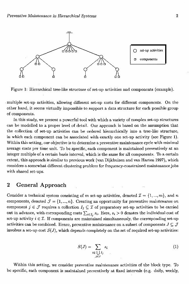
Figure 1: Hierarchical tree-like structure of set-up activities and components (example).

multiple set-up activities, allowing different set-up costs for different components. On the other hand, it seems virtually impossible to support a data structure for each possible group of components.

In this study, we present a powerful tool with which a variety of complex set-up structures can be modelled to a proper level of detail. Our approach is based on the assumption that the collection of set-up activities can be ordered hierarchically into a tree-like structure, in which each component can be associated with exactly one set-up activity (see Figure 1). Within this setting, our objective is to determine a preventive maintenance cycle with minimal average costs per time unit. To be specific,. each component is maintained preventively at an integer multiple of a certain basis interval, which is the same for all components. To a certain extent, this approach is similar to previous work (van Dijkhuizen and van Harten 1997), which considers a somewhat different clustering problem for frequency-constrained maintenance jobs with shared set-ups.

2 General Approach

Consider a technical system consisting of m set-up activities, denoted I = {I, ... , m}, and n components, denoted J = {I, ... , n}. Creating an opportunity for preventive maintenance on component j E J requires a collection Ij ~ I of preparatory set-up activities to be carried out in advance, with corresponding costs 'EiEIj Si. Here, Si > 0 denotes the individual cost of set-up activity i E If components are maintained simultaneously, the corresponding set-up activities can be combined. Hence, preventive maintenance on a subset of components J ~ J involves a set-up cost S( J), which depends completely on the set of required set-up activities:

S(J) = L Si

iE U Ij ,iEJ

(1)

Within this setting, we consider preventive maintenance activities of the block type. To be specific, each component is maintained preventively at fixed intervals (e.g. daily, weekly,


Table 1: Example of a maintenance cycle with m = n = 3, kl = 1, k2 = 3, and k3 = 8 : .6.1 (k) = 1, .6.2 (k) = 5/12, .6.3 (k) = 1/8.

components 2 2

111 1 1 1 1 set-up activities

2 2 1 1 1 1 1 1 1 frequencies

3 3 1 1 1 111 1

3 2 111 3 2 2 111

8 3 111

1

1

1

2 1

2 1

3 1

1 1

1 1

1 1

2 3 1 1

3 2 2 1 1

3 8 1 1

2 111

2 111

3 111

2 1 1

2 1 1

3 1 1

1

1

1

3 2

1 1 3 2

1 1 8 3

1 1

monthly, yearly), whereas corrective maintenance is carried out upon failure. With <Pj(x}, we denote the expected maintenance costs (exclusive of preventive set-up costs) of component j E :T per unit of time, if maintained preventively every x > 0 time units. For notational convenience, and without loss of generality, we restrict ourselves to cost functions of the following type:

<Pj(X) = Cj + Mj(x) x

(2)

Here, Cj > 0 reflects the expected cost of preventive maintenance on component j E :T. Moreover, Mj(x) denotes the expected cumulative deterioration costs of component j E :T (due to failures, repairs, etc.), x time units after its last preventive maintenance. By doing this, a variety of maintenance models can be incorporated, allowing different models for each component. The reader is referred to Dekker (1995) for an extensive list of block-type models.

2.1 Notation

Throughout this paper, we will use the following notation in order to identify the relationships between set-up activities and components in the maintenance tree (see Figure 1). As a starting point, we denote with Ij ~ I the subset of set-up activities i E I that are required for component j E :T. Similarly, we let Ji ~ :T denote the subset of components j E :T that require set-up activity i E I. Moreover, Jt ~ :T denotes the subset of components j E Ji

that are attached to set-up activity i E I. Finally, 8i ~ I represents the successors of set-up activity i E I. As an example, consider the maintenance cycle of Table 1. Then it is easily

verified that h = {I}, h = {1,2}, and 13 {I, 2, 3}. Moreover, J1 = {I, 2, 3}, h = {2,3}, and J3 {3}, whereas Ji = {I}, J2 = {2}, and J;' = {3}. Finally, we have 81 {2}, 82 = {3}, and 83 = 0.


2.2 Problem definition

The coordination of preventive maintenance activities is now modelled as follows: preventive maintenance on component j E J is carried out every kj . t time units, where kj E N*

reflects the frequency of component j relative to a basis maintenance interval of t > 0 time units, which is the same for all components. As a starting point, we consider the case where both the maintenance interval t and the maintenance frequencies kj must be chosen from a finite set of possibilities, say t E 7 and kj E JC for all j E J. In general, this yields an optimization problem in n + 1 variables (t, kl' ... , kn ), where our objective is to minimize average maintenance costs per unit of time:

(P) • . {'" Si' Ll.i(k) "'.if.. (k .)} mm mm L..J + L..J '*' j j.' t tET kjEK iEI t jE.7 .

(3)

Here, Ll.i(k) represents the fraction of times that set-up i E I is carried out at an occasion for preventive maintenance (see Table 1). For notational convenience, let us now denote with Ji = {j E J liE Ij} the set of components that require set-up activity i E I. Then it is easily observed that max{kjl I j E Ji} :::; Ll.i(k) :::; 1, implying that Ll.i(k) = 1 if kj = 1 for some j E k In general, we have the following expression for Ll.i(k) (cf. Dagnupar 1982). Here, lcm(kl' ... , kn ) represents the least common multiple of the integers kI, ... , kn :

Pil Ll.i(k) = L:( _l)l+1 L: lcm(kjp ... , kjJ-l (4)

l=1 {iI, ... ,M~Ji

Typically, the basis maintenance interval t is restricted to several days or weeks, whereas the corresponding maintenance cycle lcm(kl' ... , kn ) . t varies from several weeks to several months, or even years. In particular, this phenomenon can be observed in calendar-based maintenance planning systems, by which workload and capacity profiles have to be matched on a regular basis. There are situations, however, where there is no explicit need for this kind of regulation. In such cases, our optimization problem becomes even more complex:

(Q) (5)

A typical example of this type can be found in e.g. aircraft maintenance, where the initiation of expensive maintenance activities is usually based on flight hours. In such case~, the need for well-defined maintenance intervals (e.g. multiples of 100 flight hours) is often motivated by intuitive reasoning.


2.3 Literature

The idea of planning maintenance at integer multiples of a certain basis interval originates from multi-item inventory theory (cf. Bomberger 1966), where cost savings can be obtained by coordinating replenishment of several items. It was introduced into maintenance modelling by Gertsbakh (1972), who considered a somewhat similar but less powerful modelling framework for multiple set-up activities. Since thEm, applications into maintenance modelling have been scarse, e.g. see Sculli and Suraweera (1979), Gits (1984) and van Dijkhuizen and van Harten {1997}. At the same time, the single set-up version of our problem (m = 1) has gained considerable attention in literature. Pioneering work on this subject was carried out by Goyal and Kusy (1985) and Goyal and Gunasekaran (1992). Just recently, Wildeman (1996) presented a mathematical framework which allows for a large class of deterioration cost functions, and solved this problem to optimality. Unfortunately, this framework is based on the assumption that the correction factor .D.(k) is equal to one in the optimal strategy. Within our setting of multiple set-up activities (m > 1), it is obvious that this assumption cannot be justified, since .D.i{k) 1 for all i E 'I would leave us with a single set-up problem. In other words, the possibility that .D.i(k) < 1 for some i E 'I is essential in our approach. In general, finding the optimal maintenance strategy with correction fador is a very complex problem, even in case of a single set-up activity (cf. Goyal 1982).

2.4 Outline

The outline of this paper is as follows. In section 3, we will show that problem (P) can be formulated in terms of a surprisingly efficient mixed integer linear program. Subsequently, an heuristic approach for problem (Q) is presented in section 4. This approach is based on decomposition of· problem (Q) into three subproblems: one that determines an initial value for t, denoted (Q rel); one that determines the optimal values of (kb ... , kn) given t, denoted (Qk); and one that determines the optimal value of t given (kl' ... , kn ), denoted (Qt). In section 5, our heuristic approach is illustrated by means of a numerical example. Moreover, computational results in section 6 indicate that near-optimal solutions are obtained within reasonable CPU times. Finally, some concluding remarks are summarized in section 7.

3 Analysis of problem (P)

In this section, we will show that problem (P) can be formulated in terms of a surprisingly efficient mixed integer linear program. For notational convenience, and without loss of generality, a less efficient but more insightful version is presented first. Subsequently, two reduction techniques are presented which strongly reduce the size of this problem, in particular if the set of possible frequencies 1C is large.

3.1 Problem decomposition

First of all, let us denote with 10 = 11 n ... n In the set of common set-up activities, i.e. set-up activities that are required for each component. Then we can assume without loss of


-

·1···· ........... ~·················d/ \.~ .................. ~ ......... .

0····· ······0

o set-up activities

o components

o subtrees

Figure 2: General structure of the maintenance tree (example).

generality that 1101 = 1. To see this, 10 = 0 implies that there is no common set-up activity, in which case the maintenance tree can be decqmposed into two or more subtrees which can be treated separately. On the other hand, 1101 > 1 implies the existence of two or more common set-up activities, which obviously can be merged to a single set-up activity without affecting the problem (see Figure 2). For similar reasons, we can assume that Jt=l- 0 for all i E I.

3.2 A mixed integer linear programming formulation

For each t E T, the assignment of maintenance frequencies k E JC to components j E .1 results in a maintenance cycle of at most lcm(JC) . t time units. Here, lcm(kI, ... , kp ) represents the least-common-multiple of the integers kl ... kp , for example lcm(2, 3, 4) 12. With C = {I, ... , Icm(JC)}, we denote the set of so-called maintenance opportunities. For notational convenience, and without loss of generality, we assume that each component is maintained preventively at the end of the maintenance cycle, i.e. at maintenance opportunity 1 = lcm(JC). In line with this, we denote with Kl = {k E JC Il mod k = O} the set of maintenance frequencies that correspond with maintenance opportunity 1 E C (e.g. Ks = K16 = {I,8} in Table 1). The problem now consists of assigning maintenance frequencies to components, in such a way that the costs of the corresponding maintenance cycle are minimized. In our model, the assignment of set-up activities to maintenance opportunities is comprised into variables Xii,

with i E I and I E C, whereas the assignment of maintenance frequencies to components is represented by variables Yjk, with j E .1 and k E JC:

Xu -

Yjk =

{~ if set-up i E I is assigned to opportunity 1 E C

otherwise

{I if component j E .1 is assigned to frequency k E JC

o otherwise

With ail > 0 we denote the average cost per time unit of assigning set-up activity i E I to maintenance opportunity l E C. Similarly, bjk > 0 denotes the average cost per time unit of assigning maintenance frequency k E JC to component j E.1. With this in mind, the following expressions for ail and bjk are easily verified:


(6)

(7)

With ail and bjk as defined above, our problem can now be formulated in terms of a rather straightforward and inefficient mixed integer linear program, where our objective is to minimize average maintenance costs per unit of time:

Minimize L L ail' Xii + L L bjk . Yjk iEI lEe. jE.7 kElC

Subject to (a) Xii > Xi'I for all i E I, I E C, i' E Si

(b) Xii > Yjk for all i E I,l E C,j E Jt,k E Kl (8)

(c) L Yjk = I for all j E :1 kElC

(d) Xii > 0 for all i E I, I E C

(e) Yjk E {O,I} for all j E :1, k E Ie

Here, restrictions (a) and (b) reflect that the assignment of a certain frequency to a certain component requires the corresponding set-up activities to be carried out at the corresponding maintenance opportunities too. Moreover, restrictions (c) and (e) guarantee that exactly one frequency is assigned to each component. As a consequence, restriction (d) is sufficient to ensure that Xii E {O, I} for all i E I and I E C.

3.3 Problem reduction

Since the number of maintenance opportunities lcm(kI, ... , kp ) grows exponentially with the set of possible maintenance frequencies Ie = {kl' ... , kp}, it seems worthwile to provide a more efficient mixed integer linear programming formulation. This can be done by observing that:

(i) maintenance opportunities 1 E C with K, 0 can be left out of consideration, since evidently Xil = 0 for all i E I in any optimal solution to (8);

(ii) maintenance opportunities h, I2 E C, with Kh = Klz and II =f:. l2' can as well be replaced by a single maintenance opportunity I with KI = Kh = Kl2 and corresponding cost ail = ailt + ail2 for all i E I, since evidently Xii! = xilz for all i E I in any optimal solution to (8).


Obviously, observations (i) and (ii) may lead to significant reductions in the problem size. To be specific, if we denote with 'Fl(U) the number of times that frequency cluster U ~ /C shows up in the maintenance cycle (e.g. 'Fl{I,3} = 7 and 'Fl{I,8} = 2 in Table 1), then obviously the number of opportunities 1£*1 in the reduced version of the problem equals the number of clusters U ~ /C with 'Fl(U) > o. In general, 'l7(U) yields an expression which is similar to (4):

(9)

In general, the determination of 'l7(U) for all U ~ /C with the use of (9) is a complex problem, since the number of clusters U ~ /C grows exponentially with the number of possible maintenance frequencies /C. For similar reasons, enumeration of all maintenance opportunities is not desirable. Apparently, an efficient method has to be constructed. In this respect, it seems useful to observe that 'Fl(U) > 0 if and only if lcm(U) mod k =1= 0 for all k E /C \ u. By doing this, the majority of clusters can be discarded beforehand. Moreover, the remaining clusters can be evaluated by means of the following implicit relation, which holds for all U ~ /C. Here, we define lcm(0) = 1 for notational convenience:

lcm(U)· L 'l7(V) lcm(/C) V2U

(10)

Our analysis now proceeds as follows. As a starting point, the set of maintenance frequencies /C = {kl' ... , kp } is ordered such that kl < ... < kp • Subsequently, f!i is defined as the collection of clusters U ~ {kl' ... , kd with 'l7(U) > 0, in case the set of possible maintenance frequencies would be reduced to /C = {kI, ... , kd. Obviously, we have f! 1 = {{ I}} if kl = 1, and f!l = {0, {kd} otherwise. Since we are mainly interested in f!p, it is now sufficient to formulate an (efficient) procedure which constructs f!iHJrom f!i' It is easily verified that this can be done in the following, rather straightforward way. Starting with f!iH = 0, it is determined for each U E f!i whether (i) lcm(U) mod kiH =1= 0, and (ii) lcm(U U {ki+d) mod k =1= 0

for all k E {kI, ... , ki } \ u. If condition (i) is satisfied, f!iH is extended with cluster U. Moreover, if condition (ii) is satisfied, f!iH is extended with cluster uu {ki+d. Once f!p has been determined, the values of 'Fl(U) for all U E f!p are easily obtained by recursion:

'Fl(U) = lcm(/C) - L 'Fl(V) lcm(U) VEOp:V::::>U

(11)

As an example, consider the maintenance cycle of Table 1, with /C = {I, 3, 8}. Then it is easily verified that f!l = {{I}}, f!2 = {{l}, {I, 3}}, and f!3 = {{I}, {I, 3}, {I, 8}, {I, 3, 8}}. Starting with 'Fl{l, 3, 8} = 1 by definition, the remaining clusters are evaluated as follows:

'l7{l,3} = lcm(l, 3, 8)/lcm(l, 3) - 'Fl{l, 3, 8} 24/3 - 1 = 7,

Preventive Maintenance in Hierarchical Systems

Table 2: Reductions in

n=l

1£1 1 2 1 2 4

n=5 60 12

n= 10 2520 48

71{1,8} = km(1, 3, 8)Jkm(1, 8) 11{1, 3, 8} = 24/8 - 1 = 2,

n=

192 2880

71{1} = Icm(1, 3, 8)/km(1) 11{1,3} - 7']{1, 8} - 7']{1, 3, 8} = 24/1 - 7 2 1 = 14.

9

Clearly, this approach yields an alternative problem formulation with significantly less variables and constraints. In general, the reductions in problem size increase exponentially with the number of possible maintenance frequencies (see Table 2). Of course, our MILP formulation was tested on a series of randomly created test problems. For the outcomes of

these numerical experiments, we refer to the computational results in section 6. Here, we only mention that the LP-relaxation of problem (8) often generates an integer, and thus feasible solution to problem (P). In our view, this phenomenon is caused by the fact that our clustering problem is closely related to the standardcassignment problem, which is known to possess the above-mentioned property.

4 Analysis of problem (Q)

In general, problem (Q) is of a very complex nature, and can only be solved by local search techniques (e.g. simulated annealing). Under some weak conditions, however, its complexity can be reduced significantly. In this section, we will present an heuristic approach to problem

(Q), which is based on the assumptions mentioned below.

4.1 Model assumptions

To simplify our analysis, we assume that Mj(x) is (i) twicely differentiable, (ii) strictly positive, (iii) strictly increasing, and (iv) strictly convex on (0, (0), for all j E j. From a practical

point of view, these assumptions are related to an increasing (marginal) cost rate for postponing preventive maintenance activities (cf. Berg 1980). From a theoretical point of view, they

enable us to formulate some efficient solution procedures from convex analysis. Moreover, they account for a large class of preventive maintenance models of the block type, including

the minimal repair model (Barlow and Hunter, 1960), the standard inspection model (Barlow

et al., 1963), and the delay time model (Christer and Waller, 1984). On the other hand, if one or more components are modelled according to a standard block replacement model (Barlow

and Proschan, 1965), assumption (iv) may not be satisfied. In that case, our methods can

still be used to obtain approximate results.

Lemma 1 If Mj(x) is twicely differentiable, strictly positive, strictly increasing and strictly

convex on (0, (0), then <Pj(x) has exactly one local minimum xj < 00. Moreover, <Pj{1/x) is a convex function on (0, (0).


Proof. As a starting point, observe that x; must at least satisfy <Pj(x;) = 0 and <Pj(x;) > 0,

which is equivalent to Mj(x;) = <Pj(x;) and Mj'(x;) > O. Since <Pj(x;) < 00 by definition, and Mj(x) is strictly increasing in x, this implies the uniqueness of x;' For similar reasons,

limx-*oo Mj(x) = 00 yields x; < 00. Moreover, since fjy<Pj(l/x) = M"(x)/x3 , we also have

that fjy<Pj(l/x) ~ 0 for all x E (0,00), and thus <Pj(l/x) is a convex function on (0,00). 0

4.2 Alternative formulation

As a result of Lemma 1, it seems reasonable to rewrite our problem by transformation of t into rl in (5). By doing this, the objective function becomes a convex function in t, which obviously is a useful property in finding the optimal preventive maintenance cycle. In this alternative formulation, preventive maintenance on component j E .1 is carried out every

kj /t time units, where kj E N* denotes the frequency of component j E .1 relative to a basis maintenance interval of rl > 0 time units:

(Q) (12)

4.3 Problem relaxation

In this section, we will present a relaxation of problem (Q), which enables us to construct a lower bound for the optimal solution with the use of standard search techniques. To a certain extent, this analysis is similar to Wildeman (1996), who considers the case of a single set-up

activity (m=l). However, it contains some interesting new elements, which are typical for

our setting of multiple set-up activities. As a starting point, define scalars 0 ::; O'.ij ::; 1, such

that LiElj O'.ij = 1 for all j E .1, and observe that the following relation holds:

L <pj(kj/t) = L L O'.ij . <pj(kj/t) = L L O'.ij . <pj(kj/t) (13) jE.7 jE.7 iElj iEI jEJ;

Here, O'.ij could be interpreted as the contribution of set-up activity i E I j to the costs of component j E .1. With A ~ ~~m, we denote the set of feasible solutions to (all, ... , O'.mn).

For each 0'. E A, this yields an alternative formulation for problem (Q), in which the individual costs of each component are divided among the corresponding set-up activities:

(14)

To continue our analysis, we substitute ti = ~i(k) . t in equation (14), and observe that ti ~ tj if j E Si, since obviously ~i(k) ~ ~j(k) if set-up activity i E I is a parent of set-up

activity j E I. If we denote with T ~ ~+ the set of feasible solutions to (tl' ... , tm ), this


yields the following lower bound for problem (14):

min min'" {s .. t· + '" (¥ ..• ·(k· . b.'(k)/t.)} t T k· w* L..J z Z L..J lJ J J 1 1 EJE iEI jEJ;

(15)

. Now we substitute kij = kj . b.i(k) in equation (15), and observe that kij ~ 1 for all i E I

and j E Ji, since b.i(k) ~ kjl for all j E Ji by definition. Again, this yields an alternative lower bound for problem (15):

min min'" {so . t· + '" (¥ ..• ·(k· ./t.)} tET k .. >l L..J t t L..J tJ J lJ 1 'J- iEI jEJ;

(16)

For notational convenience, and without loss of generality, let us now define functions ej(t) = min{j(x/t)lx ~ I} for all j E.1. Since j(') attains its (unique) minimum at xj < 00, and j{l/x} is convex on (O,oo), this yields a decreasing and convex function in t:

if t < l/xj

if t ~ 1/x; (17)

Since we are free to choose (¥ E A arbitrarily, this leaves us with the following lower bound for problem (Q). Obviously, this lower bound reflects a decomposition into m interrelated subproblems, each corresponding with a single set-up activity, and its adjacent components:

(18)

Our analysis now proceeds as follows. Since ej(t) is a decreasing function in t for all j E :1, and ti ~ tj if j E Si, it can easily be verified that the optimal values of (¥ij in equation (18) are determined as follows: (¥ij = 1 if j E Jt, and (¥ij = 0 otherwise. Summarizing, this leaves us with the following lower bound for problem (Q):

(19)

Since Si . ti and ej(ti) are both convex functions in ti, and T is a convex space in lR+, this yields a convex programming problem in a convex space, which can easily be solved to optimality using standard search techniques. Here, we used the gradient projection method, e.g. see Luenberger (1984).


4.4 An heuristic approach

Our heuristic approach is based on the assumption that k; = 1 for some j E .J in the optimal solution to problem (Q). In other words, we assume that L11(k) = 1 in the optimal maintenance cycle, where i 1 denotes the common set-up activity. It seems reasonable therefore to determine the optimal solution (ti, ... ,t~) to problem (Qrel), and initialize t* = ti. Our heuristic now proceeds by solving subproblems (Qk) and (Qt) iteratively, until no improvements are observed in two consecutive iterations. Here, subproblem (Qk) determines the maintenance frequencies (ki, .. " k~) given the basis maintenance interval l/t*, whereas (Qt) determines the maintenance intervall/t* given the maintenance frequencies (ki, ... , k~), In the following section, it is shown that problem (Qt) can be solved to optimality with the use of standard search techniques. Subsequently, we will show that problem (Qk) can be decomposed into a number of independent subproblems, which can be solved separately. Moreover, we will present two heuristic to solve these subproblems~ .

4.5 Analysis of problem (Qt)

If the optimal maintenance frequencies (ki, .. " k~) are known, it is possible to compute the values of .6.i (k*) beforehand for all i E X, by using an analysis similar to section 3,3, To be specific, if we denote with '/'li(0) the number of empty maintenance opportunities in a maintenance cycle with frequency set Ki = {k; I j E Ji}, it is easily verified that the following relations holds:

(20)

Hence, if we denote with si = Si ' L1i(k*) the costs associated with set-up activity i EX, problem (Q) reduces to the following optimization problem:

(21)

Since si . t and <P j (k; / t) are both convex in t, this leaves us with a convex programming problem, which can easily be solved to optimality using standard search techniques.

4.6 Analysis of problem (Qk)

If the optimal basis maintenance intervall/t* is known, problem (Q) reduces to the following optimization problem:

(22)

Preventive· Maintenance in Hierarchical Systems 13

:::::}:I::::::::::: ::::):; if::::::: ?'f:j 7:11 K~;;;;'

}:);::::::::::::::: :::::: ::::: :;:::;:::::::::::~ i* (:: :::::: 9":2 ·:9 fJ, j.:j~~;;;:::::::::::::::::::::::::::::::::::;::::::::::;:: o set-up activities

;:':::::: :::::::::::: :::::: 1';::, :;:::::':::: :::;:: :::::: ::::::: :""',:;- :::: {:::: {: :::;:{ ::::;:;::::;: ,::::; :::::::::::: :::::: ::;;;,m :::: o components ::::::::::: ::::::':::;;; ~:::: ::::1' n":,:: ::;:~;;:::: ::{ {:: ~F:!'l ;:;' :::;:::::;: ::j'.':::: ::::~~::::: ::::~ <ii:: :::::: ::::: ::::;:: :::::::,:;' :t"'( :::::. r :::::H ::::::: ::::::::::::::1:: ::::T:::; ::::::::::::::::: :J" ::in ::::::: :::::::::::::i!;; ::::::1<::: :;:::::::::: ~:;

:;:s:;:':"': .::::: ::::::::::::~ ::::,;:,::::::::: !::::~

Figure 3: Decomposition of problem (Qk) into lSI I + 1 independent subproblems.

Under the assumption that ~l(k) = 1 in the optimal solution to problem (Q), it is easily

verified that (Qk) can be decomposed into 1811 + 1 independent subproblems, which can be solved separately. To be specific, one of these subproblems corresponds to the common setup activity i 1, and its adjacent components j E Ji, whereas each of the remaining 1811 subproblems corresponds to the subtree associated with a second-level set-up activity i E 81 (see Figure 3). In general, each subproblem is similar to problem (Qk), but refers to a reduced

set of set-up activities and components. Obviously, this decomposition may lead to significant reductions in problem sizes and computation times, whatever algorithm we decide to use.

Let us now present two heuristics for problem (Qk)' In the first heuristic, we restrict ourselves to a limited set of possible maintenance frequencies, and solve this problem by means of a mixed integer linear programming formulation. In the second heuristic, we consider the case where each set-up activity must be carried out at an integer multiple of its parental set-up activity, and show that this problem can be solved by means of an efficient dynamic

programming formulation. For notational convience, we will refer to these heuristic as the linear programming heuristic, and the dynamic programming heuristic respectively.

4.6.1 A linear programming heuristic

In the linear programming heuristic (LPH), each subproblem (Qk) is solved by means of an

efficient mixed integer linear programming formulation, as was designed for problem (P). To this end, the set of possible maintenance frequencies is reduced to K, {kmin, •.. , k max },

where kmin and k max are determined as follows. For each j E .:J, we determine the optimal

maintenance interval xi if no preventive set-up costs would be charged. Similarly, we let yj denote the optimal maintenance interval for component j E Jt if preventive set-up costs Si

would be charged:

x~ = arg min J J {

CO + M.(X)} J x>o X

(23)


* . {Si + Cj + Mj{Y) } y. = arg mm J y>O y

(24)

To a certain extent, xj and yj can be interpreted as a lower and upper bound on the optimal maintenance interval for component j ~ .1. In line with this, kmin and kmax are based on the intuitive reasoning that the maintenance frequencies (ki, ... , k~) in any optimal solution to problem (Qk) will satisfy:

kmin = rp.in lxj . t*J :::; rp.in {kj} :::; ~ax {kj} :::; ~ax ryj . t*l = kmax (25) JE:T JE:T JE:T JE::T

Since Mj(-) is assumed to be strictly increasing and convex on (O, (0), it follows from Lemma 1 that 0 < xj < yj < 00 for all j E .1, and thus 0 :::; kmin :::; kmax < 00. Obviously, we do not allow kmin = 0, and in that case set kmin = 1.

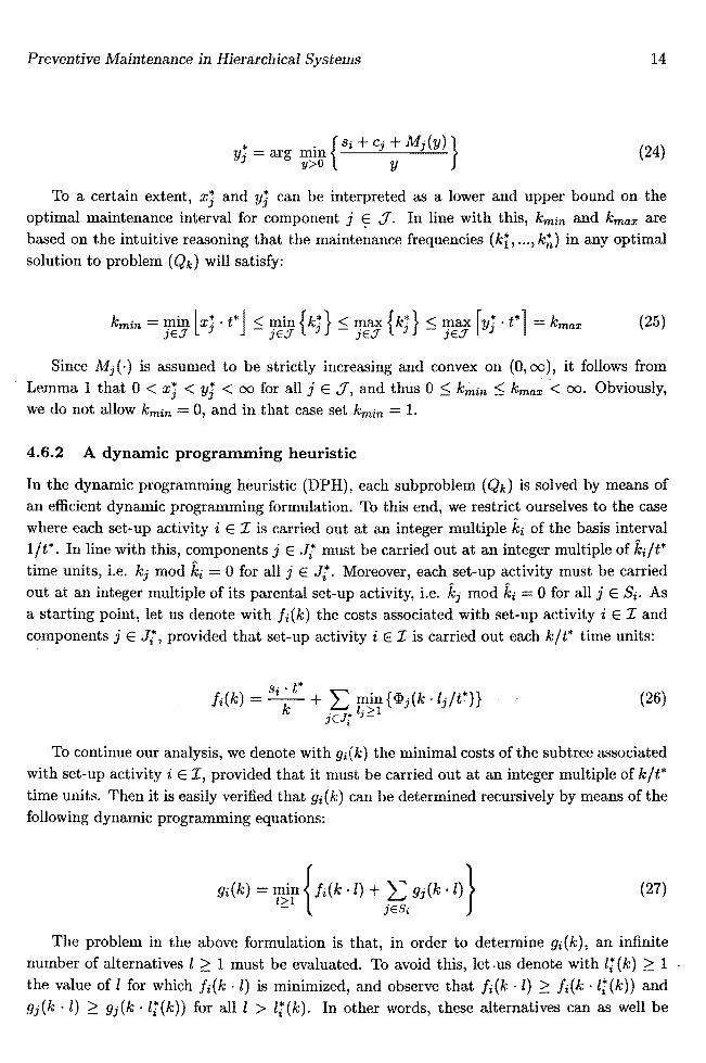
4.6.2 A dynamic programming heuristic

In the dynamic programming heuristic (DPH), each subproblem (Qk) is solved by means of an efficient dynamic programming formulation. To this end, we restrict ourselves to the case where each set-up activity i E X is carried out at an integer multiple ki of the basis interval l/t*. In line with this, components j E Jt must be carried out at an integer multiple of ki/t* time units, i.e. kj mod ki 0 for all j E Jt. Moreover, each set-up activity must be carried out at an integer multiple of its parental set-up activity, i.e. kj mod ki = 0 for all j E Si. As a starting point, let us denote with h(k) the costs associated with set-up activity i E X and components j E Jt, provided that set-up activity i E X is carried out each k/t* time units:

(26)

To continue our analysis, we denote with 9i(k) the minimal costs ofthe subtree associated with set-up activity i E X, provided that it must be carried out at an integer multiple of k/t* time units. Then it is easily verified that 9i{k) can be determined recursively by means of the following dynamic programming equations:

(27)

The problem in the above formulation is that, in order to determine 9i{k), an infinite number of alternatives I ~ 1 must be evaluated. To avoid this, let ·us denote with l;(k) ~ 1 the value of 1 for which h(k . I) is minimized, and observe that fi(k . I) ~ h(k ·li(k)) and 9j{k . I) ~ 9j{k . li(k» for alll > l;(k). In other words, these alternatives can as well be


discarded beforehand without affecting the problem. Obviously, this yields an equivalent dynamic programming formulation, in which the number of alternatives 1 ~ I ~ li(k) is finite. The question remains how to determine It(k) for all i, k. To this end, let us assume for a moment that k· It(k)/t* > xi for all j E Jt. Under this assumption, it follows from Lemma 1 that ipj{k ·l/t*) is increasing in I for alll 2:: Ii (k), and thus fi(k ·l} can be rewritten as follows:

h(k ·l) = s~'. ~* + 2: <pj(k ·l/t*) , 12:: li(k) jEJt

(28)

Let us now substitute ri = t* /(k . I) in equation {28}, and denote with rt > 0 the unique minimum of the following convex programming problem:

{29}

Since we assumed that k . It(k)/t* > xi for all j E Jt, it is now obvious that either It(k) = Lt* /(k'rt)J, or It(k) = rt* /(k. rt)l. In all other cases, we have that It(k) ~ lxi ·t* /kJ for some j E Jt. Summarizing, this leaves us with the following upper bound for li(k). Here, we denote Or = min{1/xi I j E Ji}:

Ii (k) ~ max { r k ~*rt 1 ' l k ~*or J } (30)

Hence, if we determine rt and Or for each set-up activity i E X, the dynamic programming recursion can be used to determine the optimal maintenance cycle by evaluation of 91(1).

5 Numerical Example

Consider a technical system consisting of m = 4 set-up activities and n = 4 components, with S1 = {2}, S2 = 0,83 = {4} and 84 = 0, whereas Ji {I}, J2 = {2}, J;' = {3} and Jt = {4}. For all components j E .1, the deterioration cost function ip j (.) are of the following form. Here, aj > 0, bj > 0 and Cj > 0 are strictly positive constants:

(31)

The costs Si of set-up activities i E X, as well as the parameters (aj, bj, Cj) for components j E .1, are depicted in Table 3. From these parameters, the corresponding values of xi and yj for components j E .1, as well as ti, rt and Or for set-up activities i E X are determined. Our heuristic now proceeds as follows. As a starting point, we determine the optimal solution to


Table 3: Parameter settings for numerical example. i,j Si aj bj Cj x":

1 y~

1 to:

t T~

l (r

2

1 92 453 19 3 1.679 1.758 0.569 0.527 0.596 2 64 125 14 2 1.647 1.890 0.529 0.529 0.607 3 26 252 11 1 4.786 5.027 0.365 0.288 0.209 4 15 132 23 1 2.396 2.528 0.365 0.396 0.417

Table 4: Consecutive iterations of the linear programming heuristic (LPH), and the dynamic programming heuristic (DPH), for the numerical example of Table 3.

t* {ki,···,k4} {.6.1 (k*), ... , .6.4 (k*} costs (Qk) 0.569 {1,1,3,2} {l,l'f'P 802.36

(LPH) (Qt) 0.575 {1,1,3,2} {I, l,~, 1} 802.26 (Qk) 0.575 {1,1,3,2} {I,l, I' tL 802.26 (Qk) 0.569 {1,1,2,2} {I, 1, t' f} 804.43

(DPH) (Qt) 0.562 {1,1,2,2} {I, 1, t' t} 804.29 (Qk) 0.562 {I,I,2,2} {l,I,z,z} 804.29

problem (Qre,). This yields ti = 0.569, t2 = 0.529, and ta = t! = 0.365, with corresponding lower bound 794.71. Subsequently, subproblems (Qk) and (Qt) are solved iteratively, until no improvements are observed in two consecutive iterations.

As can be observed from Table 4, the linear programming heuristic (LPH) generates a maintenance cycle of lcm{l,2, 3}/t* = 6/0.575 ~ 10.44 time units. Within this maintenance cycle, total maintenance costs amount to 10.44· 802.26 ~ 8376 on average, whereas preventive set-up costs equal 6· {92 + 64 + i ·26 + ~ ·15} = 1085, i.e. approximately 13.0% of total maintenance costs. Similarly, the dynamic programming (DPH) generate a maintenance cycle of lcm{I, 2} /t* 2/0.562 ~ 3.56 time units. Within this maintenance cycle, total maintenance costs amount to 3.56· 804.29 ~ 2863 on average, whereas preventive set-up costs equal 2· {92 + 64 + ~ . (26+ 15)} = 353, i.e. approximately 12.3% of total maintenance costs. Moreover, the performance of the (LPH) and (DPH) heuristic, i.e. the maximal deviation with respect to their lower bound, equals 0.95% and 1.21% respectively.

6 Computational results

In this section, we will discuss the results of a series of numerical experiments, which were carried out to investigate the performance of both heuristics, expressed in quantitative as well as qualitative measures. To be specific, we tested our heuristics on several test problems, in which the number of set-up activities, the number of components, and the corresponding costs were varied randomly. In order to prevent .6.i (k) = 1 for all i E I as much as possible, we decided to attach exactly one component to each set-up activity. As a consequence, the number of set-up activities equals the number of components in each test problem, which in fact were drawn at random between 1 and 50. Moreover, set-up activities were attached to each other by chosing the parent of set-up activity i randomly among set-up activities j < i.


Table 5: Computational results for the linear progamming heuristic (LPH), and the dynamic programming heuristic (DPH), based on 1000 randomly generated 'small' test problems with Si E (1,100), aj E (100,500), bj E (10,50), and Cj E (1,5).

(LPH) maximal

'11 CPU time (s) 0.00 5.78 72.86 0.00 0.06 0.44

performance (%) 0.00 2.42 12.69 0.00 2.42 12.69 interval length 0.84 1.25 4.36 0.84 1.25 4.36

cycle length 1.03 10.89 117.69 1.03 10.89 117.69

6.1 Small test problems

First of all, we investigated the performance of both heuristics for a series of small test problems, i.e. problems which can be solved by both heuristics within reasonable computation times. Obviously, this requires that the set of possible maintenance frequencies does not become too large. This was achieved by choosing Si, aj, bj and Cj in such a way that the corresponding values of xj and yj were not subject to extreme fluctuations. To be specific, the costs of set-up activities i E I were drawn at random from Si E (1,100), whereas the costs of component j E .:1 were drawn at random from aj E (100,500), bj E (10,50), and Cj E (1,5). As a consequence, xj E (0.86,7.07) and yj E (0.86,7.75) for all j E .:1.

From the results in Table 5, it can be concluded that the difference between the (LPH) and (DPH) heuristic is very small. In fact, a closer look at the results showed that both heuristics generated identical maintenance cycles in 971 out of 1000 test problems. In the remaining 29 test problems, the linear programming heuristic (LPH) outperformed the dynamic programming heuristic (DPH) in 28 cases, with a maximum of 0.26%. Apparently, the underlying structure between the dynamic programming heuristic does not affect the problem significantly. With respect to the (guaranteed) performance of both heuristics, we claim that an average deviation of 2.42% from the lower bound is quite satisfactorily. Moreover, a closer look at the results showed that in only 29 out of 1000 test problems, the performance was worse than 5%.

6.2 Large test problems

As mentioned before, the use of the linear programming heuristic (LPH) becomes undesirable if the set of possible frequencies becomes too large, e.g. Ie = {I, ... , 100}. In that case, we have to use the dynamic programming heuristic (DPH), in order to obtain reasonable solutions within acceptable computation times. To this end, we carried out another series of 1000 test problems, in which the costs of set-up activities i E I were drawn at random from Si E (1,1000). Moreover, the costs of component j E .:1 were drawn at random from aj E (1,1000), bj E (1,100), and Cj E (1,10). As a consequence, xj E (0.10,31.62) and yj E (0.14,44.72) for all j E.:1, which clearly complicates the problem.

From the results in Table 6, it can be observed that the number of iterations as well as the


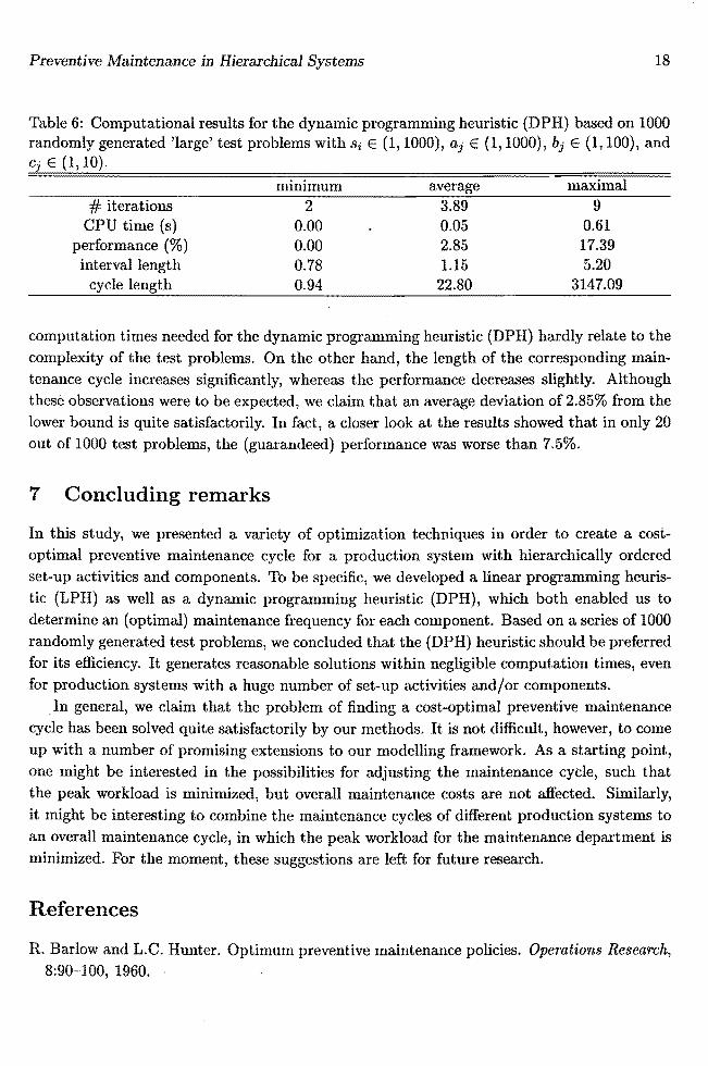
Table 6: Computational results for the dynamic programming heuristic (DPH) based on 1000 randomly generated 'large' test problems with Si E (1,1000), aj E (1,1000), bj E (1,100), and

E

average # iterations 2 3.89 9

CPU time (s) 0.00 0.05 0.61 performance (%) 0.00 2.85 17.39

interval length 0.78 1.15 5.20 0.94 22.80 3147.09

computation times needed for the dynamic programming heuristic (DPH) hardly relate to the complexity of the test problems. On the other hand, the length of the corresponding maintenance cycle increases significantly, whereas the performance decreases slightly. Although these observations were to be expected, we claim that an average deviation of 2.85% from the lower bound is quite satisfactorily. In fact, a closer look at the results showed that in only 20 out of 1000 test problems, the (guarandeed) performance was worse than 7.5%.

7 Concluding remarks

In this study, we presented a variety of optimization techniques in order to create a costoptimal preventive maintenance cycle for a production system with hierarchically ordered set-up activities and components. To be specific, we developed a linear programming heuristic (LPH) as well as a dynamic programming heuristic (DPH), which both enabled us to determine an (optimal) maintenance frequency for each component. Based on a series of 1000 randomly generated test problems, we concluded that the (DPH) heuristic should be preferred for its efficiency. It generates reasonable solutions within negligible computation times, even for production systems with a huge number of set-up activities and/or components.

In general, we claim that the problem of finding a cost-optimal preventive maintenance cycle has been solved quite satisfactorily by our methods. It is not difficult, however, to come up with a number of promising extensions to our modelling framework. As a starting point, one might be interested in the possibilities for adjusting the maintenance cycle, such that the peak workload is minimized, but overall maintenance costs are not affected. Similarly, it might be interesting to combine the maintenance cycles of different production systems to an overall maintenance cycle, in which the peak workload for the maintenance department is minimized. For the moment, these suggestions are left for future research.

References

R. Barlow and L.C. Hunter. Optimum preventive maintenance policies. Operations Research, 8:9()-'-100, 1960.


R.E. Barlow, L.C. Hunter, and F. Proschan. Optimum checking procedures. Journal of the Society for Industrial and Applied Mathematics, 4:1078-1095, 1963.

RE. Barlow and F. Proschan. Mathematical Theory of Reliability. John Wiley, New York, 1965.

M. Berg. Marginal cost analysis for preventive ·replacement policies. European Journal of Operational Research, 4, 1980.

E. Bomberger. A dynamic programming approach to the lot size scheduling problem. Management Science, 12:778-784, 1966.

D.I. Cho and M. Parlar. A survey of maintenance models for multi-unit systems. European Journal of Operational Research, 51:1-23, 1991.

A.H. Christer and W.M. Waller. Delay time models for industrial maintenance problems. European Journal of Operational Research, 35:401-406, 1984.

J.S. Dagnupar. Formulation of a multi item single supplier inventory problem. Journal of the Operational Research Society, 33:285-286, 1982.

R Dekker. Integrating optimisation, priority setting, planning and combining of maintenance activities. European Journal of Operational Research, 82:225-240, 1995.

R Dekker. Applications of maintenance optimization models: a review and analysis. Reliability engineering & system safety, 51(3):229-240, 1996.

I.B. Gertsbakh. Optimum choice of preventive maintenance times for a hierarchical system. Automated Control Computer Sciences, (6):24-30, 1972.

C.W. Gits. On the maintenance concept for a technical system. PhD thesis, University of Eindhoven, The Netherlands, 1984.

S.K. Goyal. A note on formulation of the multi-item single supplier inventory problem. Journal of the Operational Research Society, 33:287-288, 1982.

S.K. Goyal and A. Gunasekaran. Determining economic maintenance frequency of a transport fleet. International Journal of Systems Science, 4:655-659, 1992.

S.K. Goyal and M.I. Kusy. Determining economic maintenance frequencies for a family of machines. Journal of the Operational Research Society, 36(12}:1125-1128, 1985.

D.G. Luenberger. Linear and Nonlinear Programming. Addison-Wesley Publishing Company, 1984.

J.J. McCalL Maintenance policies for stochastically failing equipment: a survey. Management Science, 11:493-524, 1965.

W.P. Pierskalla and J.A. Voelker. A survey of maintenance models: the control and surveillance of deteriorating systems. Naval Research Logistics Quarterly, 23:353-388, 1976.


D. Sculli and A.W. Suraweera. Tramcar maintenance. Journal of the Operational Research Society, 30:809-814, 1979.

Y.S. Sherif and M.L. Smith. Optimal maintenance models for systems subject to failure. Naval Research Logistics Quarterly, 28:47-74, 1981.

G.C. van Dijkhuizen and A. van Harten. OptimaL clustering of frequency-constrained maintenance jobs with shared set-ups. European Journal of Operational Research, 99(3):552-564, 1997.

S.G. Vanneste. Maintenance policies for complex systems. PhD thesis, Katholieke Universiteit Brabant, 1992.

R.E. Wildeman. The Art of Grouping Maintenance. PhD thesis, Erasmus University Rotterdam, 1996.

Documents

Coordinated planning of preventive maintenance in