Embed Size (px)
Citation preview

Jacaranda (Engineering) 3333 Mail Code Phone: 818.677.6448 E-mail: [email protected] 8348 Fax: 818.677.7062
College of Engineering and Computer ScienceMechanical Engineering Department
Notes on Engineering Analysis Revised April 26, 2010 Instructor: Larry Caretto
Coordinate Transformations
Introduction
We want to carry out our engineering analyses in alternative coordinate systems. Most students have dealt with polar and spherical coordinate systems. In these notes, we want to extend this notion of different coordinate systems to consider arbitrary coordinate systems. This prepares the way for the consideration of differential equations applied to irregular regions such as those used in finite-element computer programs. Here we focus on the coordinate transformations required to convert the differential equations, originally expressed in Cartesian coordinate systems into other systems.
Notation for different coordinate systems
The general analysis of coordinate transformations usually starts with the equations in a Cartesian basis (x, y, z) and speaks of a transformation of a general alternative coordinate system (ξ, η, ζ). This is sometimes represented as a transformation from a Cartesian system (x1, x2, x3) to the dimensionless system (ξ1, ξ2, ξ3). The latter form of the transformation allows the use of a compact notation, introduced below, known as implicit summation over repeated indices. The task of determining the new coordinate system is the task of finding the appropriate transformations ξ = ξ(x, y, z), η = η(x, y, z), and ζ = ζ(x, y, z). In the numerical subscript notation, these transformations become ξ1 =ξ1(x1, x2, x3), ξ2 =ξ2(x1, x2, x3), and ξ3 =ξ3(x1, x2, x3), These three transformations can be compactly written in vector notation: ξ = ξ(x).
In numerical analysis of complex engineering systems we have to form a mesh that fits the boundaries of the system being analyzed. In such cases, ξ, η, and ζ are the computational coordinates which typically are fit to a simple grid where ξi = i, ηj = j, and ζk = k. The maximum and minimum values of the computational coordinates occur at the physical boundaries of the item being analyzed. These computational coordinates then become the independent variables in the equations. Thus we have to transform the differential equations we are analyzing from the Cartesian coordinate system to the use of ξ, η, and ζ as the independent variables. In the discussion below we present a general way to do this transformation.
The transformation of the differential equations requires information about transformation of the space derivatives. The basic relations among the space derivatives are found from the equation for the total differential of our new coordinate, dξi, where ξi = ξi(x1, x2, x3). Those basic equations express the fact that a differential change in any of the xi coordinates in the original coordinate system can cause a differential change in one of the ξi coordinates. The general equation for dξi is given below.
3,2,13
13
32
21
1
=∂∂
=∂∂
=∂∂
+∂∂
+∂∂
= ∑=
idxx
dxx
dordxx
dxx
dxx
d jj
i
jj
j
ii
iiii
ξξξξξξξ [1]
Equation [1] is written three ways. The first form shows all terms in the equation. The second form notes that the three terms on the first equation are similar and can be regarded as a sum of three separate terms using summation index j. The final form of equation [1] is similar to the

Coordinate transformations L. S. Caretto, April 26, 2010 Page 2
second form, except that the summation sign is missing. This is a shorthand notation to simplify writing such equations. In this shorthand, there is an implied summation over the terms with the repeated index. (This is known as the Einstein summation convention.) We will use this periodically to make it easier to write such equations. The final i = 1,2,3 just before the equation number applies to all three equations for dξi; it reminds us that the equation for dξi applies for the three different values of i. In the remainder of these notes we will use often write terms in full to remind readers who are not familiar with this convention that we are actually considering several terms by the implied summation.
If we looked at the inverse problem of determining the differential changes in our original coordinate system (x1, x2, x3), from differential changes in the (ξ1, ξ2, ξ3) coordinate system, we would have the following analog of equation [1].
jj
ii
iiii dxdxordxdxdxdx ξ
ξξ
ξξ
ξξ
ξ ∂∂
=∂∂
+∂∂
+∂∂
= 33
22
11
[2]
We can write both equations [1] and [2] as matrix equations to show that the partial derivatives,
j
ixξ∂∂
andi
j
x∂∂ξ
are related to each other as components of an inverse matrix. In matrix form,
equation [1] becomes.
⎥⎥⎥
⎦
⎤
⎢⎢⎢
⎣
⎡
⎥⎥⎥⎥⎥⎥⎥
⎦
⎤
⎢⎢⎢⎢⎢⎢⎢
⎣
⎡
∂∂
∂∂
∂∂
∂∂
∂∂
∂∂
∂∂
∂∂
∂∂
=⎥⎥⎥
⎦
⎤
⎢⎢⎢
⎣
⎡
3
2
1
3
3
2
3
1
3
3
2
2
2
1
2
3
1
2
1
1
1
3
2
1
dxdxdx
xxx
xxx
xxx
ddd
ξξξ
ξξξ
ξξξ
ξξξ
[3]
Converting equation [2] to matrix form gives the following result.
⎥⎥⎥
⎦
⎤
⎢⎢⎢
⎣
⎡
⎥⎥⎥⎥⎥⎥⎥
⎦
⎤
⎢⎢⎢⎢⎢⎢⎢
⎣
⎡
∂∂
∂∂
∂∂
∂∂
∂∂
∂∂
∂∂
∂∂
∂∂
=⎥⎥⎥
⎦
⎤
⎢⎢⎢
⎣
⎡
3
2
1
3
3
2
3
1
3
3
2
2
2
1
2
3
1
2
1
1
1
3
2
1
ξξξ
ξξξ
ξξξ
ξξξ
ddd
xxx
xxx
xxx
dxdxdx
[4]
Equations [3] and [4] can only be correct if the two three-by-three matrices that appear in these equations are inverses of each other. That is, the partial derivatives are related by the following matrix inversion.
Coordinate transformations L. S. Caretto, April 26, 2010 Page 3
1
3
3
2
3
1
3
3
2
2
2
1
2
3
1
2
1
1
1
3
3
2
3
1
3
3
2
2
2
1
2
3
1
2
1
1
1
−
⎥⎥⎥⎥⎥⎥⎥
⎦
⎤
⎢⎢⎢⎢⎢⎢⎢
⎣
⎡
∂∂
∂∂
∂∂
∂∂
∂∂
∂∂
∂∂
∂∂
∂∂
=
⎥⎥⎥⎥⎥⎥⎥
⎦
⎤
⎢⎢⎢⎢⎢⎢⎢
⎣
⎡
∂∂
∂∂
∂∂
∂∂
∂∂
∂∂
∂∂
∂∂
∂∂
ξξξ
ξξξ
ξξξ
ξξξ
ξξξ
ξξξ
xxx
xxx
xxx
xxx
xxx
xxx
[5]
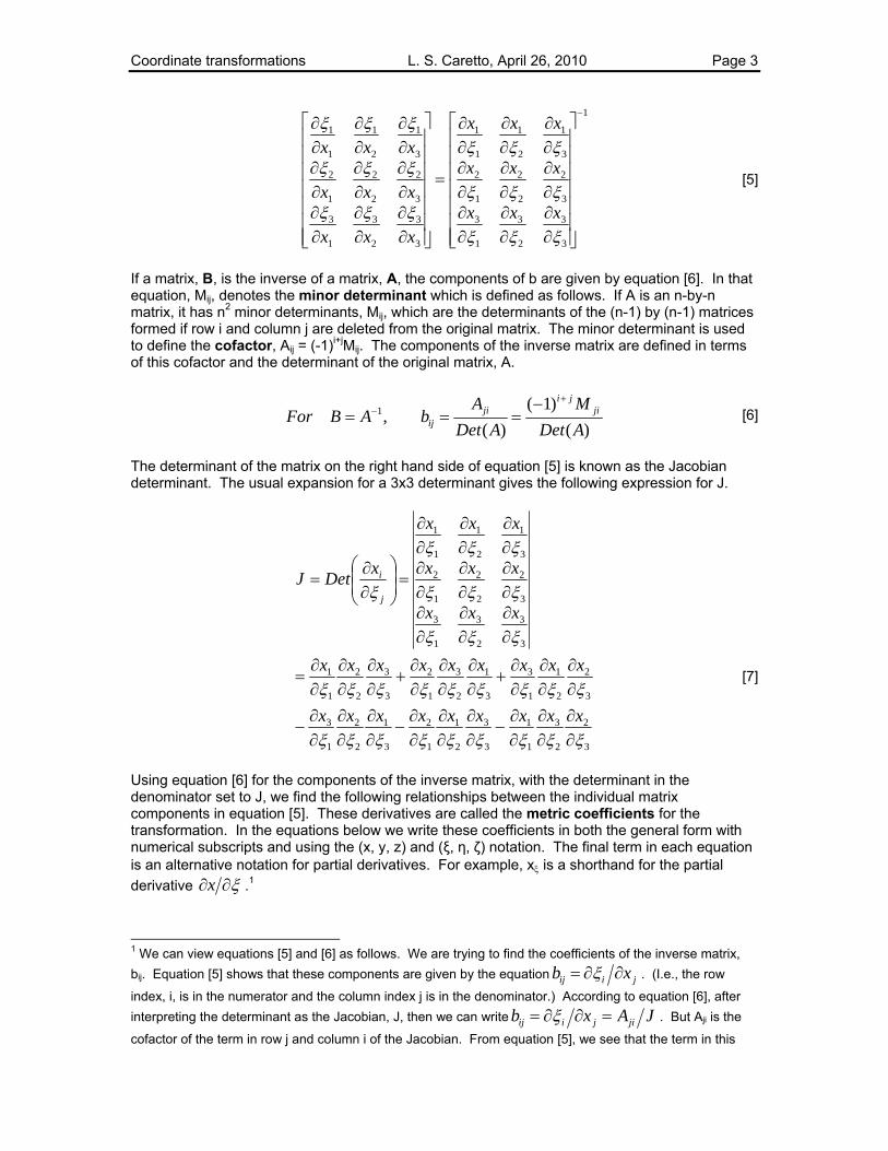
If a matrix, B, is the inverse of a matrix, A, the components of b are given by equation [6]. In that equation, Mij, denotes the minor determinant which is defined as follows. If A is an n-by-n matrix, it has n2 minor determinants, Mij, which are the determinants of the (n-1) by (n-1) matrices formed if row i and column j are deleted from the original matrix. The minor determinant is used to define the cofactor, Aij = (-1)i+jMij. The components of the inverse matrix are defined in terms of this cofactor and the determinant of the original matrix, A.
)(
)1()(
,1
ADetM
ADetA
bABFor jiji
jiij
+− −
=== [6]
The determinant of the matrix on the right hand side of equation [5] is known as the Jacobian determinant. The usual expansion for a 3x3 determinant gives the following expression for J.
3
2
2
3
1
1
3
3
2
1
1
2
3
1
2
2
1
3
3
2
2
1
1
3
3
1
2
3
1
2
3
3
2
2
1
1
3
3
2
3
1
3
3
2
2
2
1
2
3
1
2
1
1
1
ξξξξξξξξξ
ξξξξξξξξξ
ξξξ
ξξξ
ξξξ
ξ
∂∂
∂∂
∂∂
−∂∂
∂∂
∂∂
−∂∂
∂∂
∂∂
−
∂∂
∂∂
∂∂
+∂∂
∂∂
∂∂
+∂∂
∂∂
∂∂
=
∂∂
∂∂
∂∂
∂∂
∂∂
∂∂
∂∂
∂∂
∂∂
=⎟⎟⎠
⎞⎜⎜⎝
⎛
∂∂
=
xxxxxxxxx
xxxxxxxxx
xxx
xxx
xxx
xDetJj
i
[7]
Using equation [6] for the components of the inverse matrix, with the determinant in the denominator set to J, we find the following relationships between the individual matrix components in equation [5]. These derivatives are called the metric coefficients for the transformation. In the equations below we write these coefficients in both the general form with numerical subscripts and using the (x, y, z) and (ξ, η, ζ) notation. The final term in each equation is an alternative notation for partial derivatives. For example, xξ is a shorthand for the partial derivative ξ∂∂x .1
1 We can view equations [5] and [6] as follows. We are trying to find the coefficients of the inverse matrix, bij. Equation [5] shows that these components are given by the equation jiij xb ∂∂= ξ . (I.e., the row
index, i, is in the numerator and the column index j is in the denominator.) According to equation [6], after interpreting the determinant as the Jacobian, J, then we can write JAxb jijiij =∂∂= ξ . But Aji is the
cofactor of the term in row j and column i of the Jacobian. From equation [5], we see that the term in this

Coordinate transformations L. S. Caretto, April 26, 2010 Page 4
J
yzzyyzzyJx
orxxxx
Jxζηζη
ζηζηξ
ξξξξξ −
=⎥⎦
⎤⎢⎣
⎡∂∂
∂∂
−∂∂
∂∂
=∂∂
⎥⎦
⎤⎢⎣
⎡∂∂
∂∂
−∂∂
∂∂
=∂∂ 11
3
2
2
3
3
3
2
2
1
1 [8]
J
zxzxzxzxJy
orxxxx
Jxζηηζ
ζηηζξ
ξξξξξ −
=⎥⎦
⎤⎢⎣
⎡−
∂∂
∂∂
−∂∂
∂∂
=∂∂
⎥⎦
⎤⎢⎣
⎡∂∂
∂∂
−∂∂
∂∂
=∂∂ 11
3
3
2
1
2
3
3
1
2
1 [9]
J
yxyxyxyxJz
orxxxx
Jxηζζη
ηζζηξ
ξξξξξ −
=⎥⎦
⎤⎢⎣
⎡∂∂
∂∂
−∂∂
∂∂
=∂∂
⎥⎦
⎤⎢⎣
⎡∂∂
∂∂
−∂∂
∂∂
=∂∂ 11
2
2
3
1
3
2
2
1
3
1 [10]
J
zyzyzyzyJx
orxxxx
Jxζξξζ
ζξξζη
ξξξξξ −
=⎥⎦
⎤⎢⎣
⎡∂∂
∂∂
−∂∂
∂∂
=∂∂
⎥⎦
⎤⎢⎣
⎡∂∂
∂∂
−∂∂
∂∂
=∂∂ 11
3
3
1
2
1
3
3
2
1
2 [11]
J
zxzxzxzxJy
orxxxx
Jxξζζξ
ξζζξη
ξξξξξ −
=⎥⎦
⎤⎢⎣
⎡∂∂
∂∂
−∂∂
∂∂
=∂∂
⎥⎦
⎤⎢⎣
⎡∂∂
∂∂
−∂∂
∂∂
=∂∂ 11
1
3
3
1
3
3
1
1
2
2 [12]
J
yxyxyxyxJz
orxxxx
Jxξζζξ
ξζζξη
ξξξξξ −
=⎥⎦
⎤⎢⎣
⎡∂∂
∂∂
−∂∂
∂∂
=∂∂
⎥⎦
⎤⎢⎣
⎡∂∂
∂∂
−∂∂
∂∂
=∂∂ 11
1
2
3
1
3
2
1
1
3
2 [13]
J
zyzyzyzyJz
orxxxx
Jxξηηξ
ξηηξζ
ξξξξξ −
=⎥⎦
⎤⎢⎣
⎡∂∂
∂∂
−∂∂
∂∂
=∂∂
⎥⎦
⎤⎢⎣
⎡∂∂
∂∂
−∂∂
∂∂
=∂∂ 11
1
3
2
2
2
3
1
2
1
3 [14]
J
zxzxzxzxJy
orxxxxJx
ηξξη
ηξξηζ
ξξξξξ −
=⎥⎦
⎤⎢⎣
⎡∂∂
∂∂
−∂∂
∂∂
=∂∂
⎥⎦
⎤⎢⎣
⎡∂∂
∂∂
−∂∂
∂∂
=∂∂ 11
2
3
1
1
1
3
2
1
2
3 [15]
J
yxyxyxyxJz
orxxxx
Jxηξηξ
ηξηξζ
ξξξξξ −
=⎥⎦
⎤⎢⎣
⎡∂∂
∂∂
−∂∂
∂∂
=∂∂
=⎥⎦
⎤⎢⎣
⎡∂∂
∂∂
−∂∂
∂∂
=∂∂ 11
1
2
2
1
2
2
1
1
3
3 [16]]
The simpler relationships for two-dimensional coordinate systems can be found from these equations by recognizing that in such coordinates, there is no variation in the third dimension. This means that there is no variation of x or y with ζ. Thus all derivative of x and y with respect to ζ are zero. We set the derivative zζ = 1 to modify equations [8] to [16] for two-dimensional systems. This is equivalent to assuming a coordinate transformation of z = ζ for this conversion. The results of converting equations [8], [9], [11] and [12] to two-dimensional forms are shown below
Jyy
Jxor
xJx
η
ηξ
ξξ
=⎥⎦
⎤⎢⎣
⎡∂∂
=∂∂
⎥⎦
⎤⎢⎣
⎡∂∂
=∂∂ 11
2
2
1
1 [17]
position is ijx ξ∂∂ . Thus we can make the following general statement about the results shown in
equations [8] to [16]: ji x∂∂ξ equals the cofactor of ijx ξ∂∂ divided by the Jacobian, J.

Coordinate transformations L. S. Caretto, April 26, 2010 Page 5
Jxx
Jyor
xJx
η
ηξ
ξξ
−=⎥⎦
⎤⎢⎣
⎡∂∂
−=∂∂
⎥⎦
⎤⎢⎣
⎡∂∂
−=∂∂ 11
2
1
2
1 [18]
Jyy
Jxor
xJx
ξ
ξη
ξξ
−=⎥⎦
⎤⎢⎣
⎡∂∂
−=∂∂
⎥⎦
⎤⎢⎣
⎡∂∂
−=∂∂ 11
1
2
1
2 [19]
Jxx
Jyor
xJx
ξ
ξη
ξξ
=⎥⎦
⎤⎢⎣
⎡∂∂
=∂∂
⎥⎦
⎤⎢⎣
⎡∂∂
=∂∂ 11
1
1
2
2 [20]
For the two dimensional case, the Jacobian has the simple form of a two-by-two determinant.
ηξηξηξηξyxyxyxyxJ −=
∂∂
∂∂
−∂∂
∂∂
= [21]
(Note that equation [16] is correct when we convert from three dimensions to two by setting z = ζ. The left hand side, zζ, is equal to one. The terms in braces on the left-hand side are just the definition of the Jacobian, J, for the two-dimensional case. Thus both sides of equation [16] are equal to one in the two-dimensional case.)
Transforming differential equations
We are now ready to transform the various vector operators from Cartesian coordinates to our arbitrary coordinate system. We begin with the divergence because this is a transformation of first derivatives. Subsequently we will consider the Laplacian which requires a transformation of second derivatives. As usual we will regard second derivatives as first derivatives of first derivatives and be able to apply the results of the first-derivative transformations to the results for second derivatives.
Transforming the divergence
The divergence of a vector with Cartesian components F1, F2, and F3, in the x, y, and z coordinate directions (here expressed as x1, x2, and x3) is written as follows. (The second form uses the implied summation over the repeated index, i.)
i
i
xFdivor
xF
xF
xFdiv
∂∂
=∂∂
+∂∂
+∂∂
= FF3
3
2
2
1
1 [22]
In computational fluid dynamics equations, the convection terms, with Fi = ρuiφ, are given by this divergence expression.
To carry out the grid transformation for the divergence, we recognize each Cartesian coordinate can depend on all the other coordinates. Because of this, a change in any of the transformed coordinates can be reflected as a change in any of the original coordinates. We can reflect this dependence by writing the following equation to convert first derivatives in our Cartesian coordinate system (with respect to any Cartesian coordinate, xi) to first derivatives in new coordinate system where the coordinate variables are called ξ, η, and ζ or ξ1, ξ2, and ξ3 or ξj in general.

Coordinate transformations L. S. Caretto, April 26, 2010 Page 6
3,2,1=∂∂
∂∂
=∂∂
∂∂
∂∂
+∂∂
∂∂
+∂∂
∂∂
=∂∂ i
xxor
xxxx ji
j
iiiii ξξ
ζζ
ηη
ξξ [23]
The second form of this equation has an implied summation over the repeated j index. We have to apply this equation to each of the three terms in our divergence equation [22].
⎟⎟⎠
⎞⎜⎜⎝
⎛∂∂
∂∂
+∂∂
∂∂
+∂∂
∂∂
+⎟⎟⎠
⎞⎜⎜⎝
⎛∂∂
∂∂
+∂∂
∂∂
+∂∂
∂∂
+
⎟⎟⎠
⎞⎜⎜⎝
⎛∂∂
∂∂
+∂∂
∂∂
+∂∂
∂∂
=∂∂
+∂∂
+∂∂
=∂∂
=
ζζ
ηη
ξξ
ζζ
ηη
ξξ
ζζ
ηη
ξξ
3
3
3
3
3
3
2
2
2
2
2
2
1
1
1
1
1
13
3
2
2
1
1
Fx
Fx
Fx
Fx
Fx
Fx
Fx
Fx
Fxx
FxF
xF
xFdiv
i
iF [24]
We can simplify the number of terms that we have to write by using the implied summation over repeated indices of the summation convention. Here we repeat two indices, which allows us to rewrite all nine terms on the left of equation [24] in the following compact notation.
j
i
i
j Fx
Divξ
ξ∂∂
∂∂
=F [25]
The conversion of this form into a more useful result does not follow an obvious path. The initial step in the conversion is done by first multiplying by the Jacobian of the transformation, J, and applying the chain rule of differentiation to write the resulting JXdF terms as d(JFX) – Fd(JX). This gives the following result.
)()( JXFdJXFdJXdFx
JFx
JFFx
JJDivi
j
ji
i
ji
jj
i
i
j
−=
⎟⎟⎠
⎞⎜⎜⎝
⎛∂
∂
∂∂
−⎟⎟⎠
⎞⎜⎜⎝
⎛∂
∂
∂∂
=∂∂
∂
∂=
ξξ
ξξξ
ξF [26]
We continue to have two repeated indices that imply summation over both i and j. We can show that the final term, multiplied by Fi, is zero for each value of i by using the metric coefficient relationships in equations [8] to [16]. We first get the following result for i = 1, using equations [8], [11], and [14].
⎟⎟⎠
⎞⎜⎜⎝
⎛∂∂
∂∂
−∂∂
∂∂
∂∂
+⎟⎟⎠
⎞⎜⎜⎝
⎛∂∂
∂∂
−∂∂
∂∂
∂∂
+
⎟⎟⎠
⎞⎜⎜⎝
⎛∂∂
∂∂
−∂∂
∂∂
∂∂
=⎟⎟⎠
⎞⎜⎜⎝
⎛∂∂
∂∂
+⎟⎟⎠
⎞⎜⎜⎝
⎛∂∂
∂∂
+⎟⎟⎠
⎞⎜⎜⎝
⎛∂∂
∂∂
=⎟⎟⎠
⎞⎜⎜⎝
⎛∂
∂
∂∂
1
3
2
2
2
3
1
2
33
3
1
2
1
3
3
2
2
3
2
2
3
3
3
2
2
11
3
31
2
21
1
11
ξξξξξξξξξξ
ξξξξξξ
ξξ
ξξ
ξξ
ξ
xxxxxxxx
xxxxx
Jx
Jx
Jx
J j
j [27]
Carrying out the indicated differentiations gives the combination of mixed, second-order partial derivatives shown below. Each of these derivatives occurs two times, once with a plus sign and once with a minus sign. (The order of differentiation is also different, but mixed second order derivatives are the same regardless of the order of differentiation.) A letter below the term with a plus or minus sign indicates the matching terms that cancel. For example, the term labeled (+A) has a plus sign in the equation that cancels the term labeled (-A).

Coordinate transformations L. S. Caretto, April 26, 2010 Page 7
)()()()(
)()()()(
)()()()(
13
32
2
2
23
32
1
2
1
3
23
22
2
3
13
22
32
32
1
2
12
32
3
2
3
3
12
22
1
3
32
22
31
22
2
3
31
32
2
2
3
2
21
32
3
3
21
22
1
CFED
xxxxxxxxFBAE
xxxxxxxxDCBA
xxxxxxxxx
J j
j
−+−+∂∂
∂∂∂
−∂∂
∂∂∂
+∂∂
∂∂∂
−∂∂
∂∂∂
+
−+−+∂∂
∂∂∂
−∂∂
∂∂∂
+∂∂
∂∂∂
−∂∂
∂∂∂
+
−+−+
∂∂∂
∂∂
−∂∂
∂∂∂
+∂∂
∂∂∂
−∂∂
∂∂∂
=⎟⎟⎠
⎞⎜⎜⎝
⎛∂
∂
∂∂
ξξξξξξξξξξξξ
ξξξξξξξξξξξξ
ξξξξξξξξξξξξξ
ξ
[28]
This shows that the ⎟⎟⎠
⎞⎜⎜⎝
⎛∂
∂
∂∂
i
j
ji x
JFξ
ξterm in equation [45] is zero when i = 1. The proof that this
term is zero for i = 2 and i = 3 follows the same approach used above and is left as an exercise for the interested reader. With all these terms zero, equation [45] gives the following result for the transformed convection terms.
⎟⎟⎠
⎞⎜⎜⎝
⎛∂∂
∂∂
=⇒⎟⎟⎠
⎞⎜⎜⎝
⎛∂∂
∂∂
=i
ji
ji
ji
j xJF
JDiv
xJFDivJ
ξξ
ξξ
1FF [29]
We can define the components of the differentiation by ξj in the new coordinate system as follows.
3
32
21
1 xF
xF
xF
xFG jjj
i
jij ∂
∂+
∂∂
+∂∂
=∂∂
=ξξξξ
[30]
With this definition, the divergence in our new coordinate system, with the new components Gj, becomes
j
j
i
ji
j
JGJx
JFJ
Divξ
ξξ ∂
∂=⎟⎟
⎠
⎞⎜⎜⎝
⎛∂∂
∂∂
=11F [31]
Transforming the Laplacian
We can extend this result to derive a form for the Laplacian operator in the new coordinate system. The Laplacian can be viewed as the divergence of a gradient. In Cartesian coordinates the Laplacian is written as follows.
⎟⎟⎠
⎞⎜⎜⎝
⎛∂∂
+∂∂
+∂∂
==∂∂
+∂∂
+∂∂
=∇ )3(3
)2(2
)1(1
23
2
22
2
21
22 )( eee
xu
xu
xuDivugradDiv
xu
xu
xuu [32]
Here we have used e(1), e(2), and e(3) to represent the usual unit vectors i, j, and k. We see that the Laplacian represents the divergence of a vector whose components Fi = ixu ∂∂ . However,

Coordinate transformations L. S. Caretto, April 26, 2010 Page 8
we have just found an expression for the divergence in our new coordinate system by the combination of equations [30] and [31]. Applying equation [30] with Fi = ixu ∂∂ gives.
332211 xx
uxx
uxx
uxx
ux
FG jjj
i
j
ii
jij ∂
∂∂∂
+∂∂
∂∂
+∂∂
∂∂
=∂∂
∂∂
=∂∂
=ξξξξξ
[33]
We want the derivatives of u with respect to our new coordinate system. To do this we use the general relationship for partial derivatives that gives ixu ∂∂ as derivatives of the new coordinate system; we can show all terms or use the summation convention.
i
k
kiiii xu
xu
xu
xu
xu
∂∂
∂∂
=∂∂
∂∂
+∂∂
∂∂
+∂∂
∂∂
=∂∂ ξ
ξξ
ξξ
ξξ
ξ3
3
2
2
1
1
[34]
We can combine equations [33] and [34] to get a definition of Gj that involves an implied summation over the repeated indices i and k. In equation [35] we show all nine terms that result from the implied summation over these two repeated indices.
⎟⎟⎠
⎞⎜⎜⎝
⎛∂∂
∂∂
+∂∂
∂∂
+∂∂
∂∂
∂∂
+⎟⎟⎠
⎞⎜⎜⎝
⎛∂∂
∂∂
+∂∂
∂∂
+∂∂
∂∂
∂∂
+
⎟⎟⎠
⎞⎜⎜⎝
⎛∂∂
∂∂
+∂∂
∂∂
+∂∂
∂∂
∂∂
=∂∂
∂∂
∂∂
=
3
3
33
2
23
1
132
3
32
2
22
1
12
1
3
31
2
21
1
11
xu
xu
xu
xxu
xu
xu
x
xu
xu
xu
xxxuG
jj
j
i
j
i
k
kj
ξξ
ξξ
ξξ
ξξξ
ξξ
ξξ
ξ
ξξ
ξξ
ξξ
ξξξξ
[35]
With this definition for Gj, we can use equation [31] to write our Laplacian with the implied summation over the j index.
⎥⎦
⎤⎢⎣
⎡⎟⎟⎠
⎞⎜⎜⎝
⎛∂∂
∂∂
∂∂
∂∂
=∂∂
=∇i
j
i
k
kjj
j
xxuJ
JJG
Ju
ξξξξξ
112 [36]
Equation [36] has three repeated indices (i, j, and k) which imply a summation over all possible values of each index. This gives a total of 27 terms in equation [36]. The three explicit terms for j = 1, 2, and 3 are shown below. Each of these terms has an implied summation over the repeated i and k indices.
⎪⎭
⎪⎬⎫
⎪⎩
⎪⎨⎧
⎥⎦
⎤⎢⎣
⎡⎟⎟⎠
⎞⎜⎜⎝
⎛∂∂
∂∂
∂∂
∂∂
+⎥⎦
⎤⎢⎣
⎡⎟⎟⎠
⎞⎜⎜⎝
⎛∂∂
∂∂
∂∂
∂∂
+⎥⎦
⎤⎢⎣
⎡⎟⎟⎠
⎞⎜⎜⎝
⎛∂∂
∂∂
∂∂
∂∂
=∇ii
k
kii
k
kii
k
k xxuJ
xxuJ
xxuJ
Ju 3
3
2
2
1
1
2 1 ξξξξ
ξξξξ
ξξξξ
[37]
Another view of equation [36], shown below, contains all the terms for j = 1. The terms for j = 2 and j = 3 are left as an implied summation over i and k.

Coordinate transformations L. S. Caretto, April 26, 2010 Page 9
⎪⎭
⎪⎬⎫⎥⎦
⎤⎢⎣
⎡⎟⎟⎠
⎞⎜⎜⎝
⎛∂∂
∂∂
∂∂
∂∂
+⎥⎦
⎤⎢⎣
⎡⎟⎟⎠
⎞⎜⎜⎝
⎛∂∂
∂∂
∂∂
∂∂
+
⎥⎦
⎤⎟⎟⎠
⎞∂∂
∂∂
∂∂
+∂∂
∂∂
∂∂
+∂∂
∂∂
∂∂
+
∂∂
∂∂
∂∂
+∂∂
∂∂
∂∂
+∂∂
∂∂
∂∂
+
⎪⎩
⎪⎨⎧
⎢⎣
⎡∂∂
∂∂
∂∂
+∂∂
∂∂
∂∂
+⎜⎜⎝
⎛∂∂
∂∂
∂∂
∂∂
=∇
ii
k
kii
k
k xxuJ
xxuJ
xxu
xxu
xxu
xxu
xxu
xxu
xxu
xxu
xxuJ
Ju
3
3
2
2
3
1
3
3
32
1
2
3
31
1
1
3
3
3
1
3
2
22
1
2
2
21
1
1
2
2
3
1
3
1
12
1
2
1
11
1
1
1
11
2 1
ξξξξ
ξξξξ
ξξξ
ξξξ
ξξξ
ξξξ
ξξξ
ξξξ
ξξξ
ξξξ
ξξξξ
[38]
Equation [36] provides the most comprehensive form for the Laplacian in an arbitrary coordinate system. We can apply it to the simplest example of cylindrical-coordinate systems where x = r cos(θ), y = r sin(θ) and z = z. In our generalized coordinate system, the Cartesian coordinates are found from the new coordinates by the following form of these transformations: x1 = ξ1 cos(ξ2), x2 = ξ1 sin(ξ2) and x3 = ξ3. The derivatives for this system are written below.
100
0)cos()sin(
0)sin()cos(
3
3
2
3
1
3
3
221
2
22
1
2
3
121
2
12
1
1
=∂∂
=∂∂
=∂∂
=∂∂
=∂∂
=∂∂
=∂∂
−=∂∂
=∂∂
ξξξ
ξξξ
ξξ
ξ
ξξξ
ξξ
ξ
xxx
xxx
xxx
[39]
We use equation [7] to compute J using these derivatives.
[ ][ ][ ] [ ][ ][ ] [ ][ ][ ][ ][ ][ ] [ ][ ][ ] [ ][ ][ ] [ ] 12
22
21221221
21212212
3
2
2
3
1
1
3
3
2
1
1
2
3
1
2
2
1
3
3
2
2
1
1
3
3
1
2
3
1
2
3
3
2
2
1
1
)(sin)(cos00)cos(1)sin()sin(0)cos(00)sin(0)sin(0)sin(1)cos()cos(
ξξξξξξξξξξ
ξξξξξξξξξξξξξξξξξ
ξξξξξξξξξ
=+=−−−−
−+−+=∂∂
∂∂
∂∂
−∂∂
∂∂
∂∂
−∂∂
∂∂
∂∂
−
∂∂
∂∂
∂∂
+∂∂
∂∂
∂∂
+∂∂
∂∂
∂∂
=
xxxxxxxxx
xxxxxxxxxJ
[40]
We now have to use equations [8] to [16] to compute the derivatives ji x∂∂ξ from the derivatives found in equation [35] and the Jacobian.
( )( ) ( )( )[ ] )cos(001)cos(11221
13
2
2
3
3
3
2
2
1
1 ξξξξξξξξ
ξ=−=⎥
⎦
⎤⎢⎣
⎡∂∂
∂∂
−∂∂
∂∂
=∂∂ xxxx
Jx [41]
( )( ) ( )( )[ ] )sin(1)sin(0011221
13
3
2
1
2
3
3
1
2
1 ξξξξξξξξ
ξ=−−=⎥
⎦
⎤⎢⎣
⎡∂∂
∂∂
−∂∂
∂∂
=∂∂ xxxx
Jx [42]

Coordinate transformations L. S. Caretto, April 26, 2010 Page 10
( )( ) ( )( )[ ] 0)cos(00)sin(112121
12
2
3
1
3
2
2
1
3
1 =−−=⎥⎦
⎤⎢⎣
⎡∂∂
∂∂
−∂∂
∂∂
=∂∂ ξξξξ
ξξξξξξ xxxx
Jx [43]
( )( ) ( )( )[ ]1
22
13
3
1
2
1
3
3
2
1
2 )sin(1)sin(0011ξξξ
ξξξξξξ
−=−=⎥⎦
⎤⎢⎣
⎡∂∂
∂∂
−∂∂
∂∂
=∂∂ xxxx
Jx [44]
( )( ) ( )( )[ ]1
22
11
3
3
1
3
3
1
1
2
2 )cos(001)cos(11ξξξ
ξξξξξξ
=−=⎥⎦
⎤⎢⎣
⎡∂∂
∂∂
−∂∂
∂∂
=∂∂ xxxx
Jx [45]
( )( ) ( )( )[ ] 0)sin(00)cos(1122
11
2
3
1
3
2
1
1
3
2 =−=⎥⎦
⎤⎢⎣
⎡∂∂
∂∂
−∂∂
∂∂
=∂∂ ξξ
ξξξξξξ xxxx
Jx [46]
( )( ) ( )( )[ ] 00)cos(0)sin(11212
11
3
2
2
2
3
1
2
1
3 =−=⎥⎦
⎤⎢⎣
⎡∂∂
∂∂
−∂∂
∂∂
=∂∂ ξξξ
ξξξξξξ xxxx
Jx [47]
( )( ) ( )( )[ ] 00)cos(0)sin(11221
12
3
1
1
1
3
2
1
2
3 =−−=⎥⎦
⎤⎢⎣
⎡∂∂
∂∂
−∂∂
∂∂
=∂∂ ξξξ
ξξξξξξ xxxx
Jx [48]
( )( ) ( )( )[ ] 1)sin()sin()cos()cos(11221212
11
2
2
1
2
2
1
1
3
3 =−−=⎥⎦
⎤⎢⎣
⎡∂∂
∂∂
−∂∂
∂∂
=∂∂ ξξξξξξ
ξξξξξξ xxxx
Jx[49]]
Before substituting these derivatives into equation [36] we note that we can rewrite equation [36] as follows, defining Bkj as the product of two different partial derivatives with respect to xi summed over all three values of i.
i
j
i
kkj
kkj
ji
j
i
k
kj xxBwhereuJB
JxxuJ
Ju
∂∂
∂∂
=⎟⎟⎠
⎞⎜⎜⎝
⎛∂∂
∂∂
=⎥⎦
⎤⎢⎣
⎡⎟⎟⎠
⎞⎜⎜⎝
⎛∂∂
∂∂
∂∂
∂∂
=∇ξξ
ξξξξ
ξξ112 [50]
We can write the explicit definition of Bkj (without the implied summation) as follows. Note that Bkj = Bjk.
332211 xxxxxxxx
B jkjkjk
i
j
i
kkj ∂
∂∂∂
+∂∂
∂∂
+∂∂
∂∂
=∂∂
∂∂
=ξξξξξξξξ [51]
Using the derivatives in equations [41] to [49] (and the result that J = ξ1), we can write the factor Bkj from equation [50].
10)(sin)(cos 22
22
3
1
3
1
2
1
2
1
1
1
1
111 =++=
∂∂
∂∂
+∂∂
∂∂
+∂∂
∂∂
= ξξξξξξξξxxxxxx
B [52]

Coordinate transformations L. S. Caretto, April 26, 2010 Page 11
00)cos()sin()sin()cos(1
22
1
22
3
2
3
1
2
2
2
1
1
2
1
11221 =+⎟⎟
⎠
⎞⎜⎜⎝
⎛+⎟⎟
⎠
⎞⎜⎜⎝
⎛ −=
∂∂
∂∂
+∂∂
∂∂
+∂∂
∂∂
==ξξξ
ξξξξξξξξξ
xxxxxxBB [53]
( ) ( ) 0)1)(0(0)sin(0)cos( 223
3
3
1
2
3
2
1
1
3
1
11331 =++=
∂∂
∂∂
+∂∂
∂∂
+∂∂
∂∂
== ξξξξξξξξxxxxxx
BB [54]
21
22
1
2
2
1
2
3
2
3
2
2
2
2
2
1
2
1
222
10)cos()sin(ξξ
ξξξξξξξξξ
=+⎟⎟⎠
⎞⎜⎜⎝
⎛+⎟⎟
⎠
⎞⎜⎜⎝
⎛ −=
∂∂
∂∂
+∂∂
∂∂
+∂∂
∂∂
=xxxxxx
B [55]
( ) ( ) 0)1)(0(0)cos(0)sin(
1
2
1
2
3
3
3
2
2
3
2
2
1
3
1
22332 =+⎟⎟
⎠
⎞⎜⎜⎝
⎛−+⎟⎟
⎠
⎞⎜⎜⎝
⎛−=
∂∂
∂∂
+∂∂
∂∂
+∂∂
∂∂
==ξξ
ξξξξξξξξ
xxxxxxBB [56]
1100 222
3
3
3
3
2
3
2
3
1
3
1
333 =++=
∂∂
∂∂
+∂∂
∂∂
+∂∂
∂∂
=xxxxxx
B ξξξξξξ [57]
We see that all the values of Bjk are zero unless j = k. This will always be the case for an orthogonal coordinate system. For such a system we can rewrite equation [50] to set all terms where j ≠ k to zero.
⎟⎟⎠
⎞⎜⎜⎝
⎛∂∂
∂∂
+∂∂
∂∂
+∂∂
∂∂
=∇3
3332
2221
111
2 1ξξξξξξuJBuJBuJB
Ju [58]
Using the values of B11, B22, and B33, from equations [52], [55], and [57], and the result from equation [40] that J = ξ1., we can write our Laplacian for cylindrical polar coordinates.
⎟⎟⎠
⎞⎜⎜⎝
⎛∂∂
∂∂
+∂∂
∂∂
+∂∂
∂∂
=∇3
132
21
121
111
2 )1(1)1(1ξ
ξξξξ
ξξξ
ξξξ
uuuu [59]
Since the three coordinate directions are independent we can remove the x1 terms from the x2 and x3 derivatives and finally use the conventional r, θ, z coordinates to give the final result for the Laplacian in cylindrical coordinates.
2
2
2
2
223
2
22
2
211
111
2 1111zuu
rrur
rruuuu
∂∂
+∂∂
+∂∂
∂∂
=∂∂
+∂∂
+∂∂
∂∂
=∇θξξξξ
ξξξ
[60]
Laplace’s equation with variable properties
As noted above, the Laplacian can be viewed as the divergence of a gradient. Typically the gradient times some physical coefficient, Γ, represents a flux term. If the physical coefficient is constant, we can bring it outside the outer divergence operator and merge it with other terms in the equation. However, if Γ is not a constant, we have to leave it inside the outer divergence operator. In this case, we replace equation[ 32] with the following equation in Cartesian coordinates.

Coordinate transformations L. S. Caretto, April 26, 2010 Page 12
⎥⎦
⎤⎢⎣
⎡⎟⎟⎠
⎞⎜⎜⎝
⎛∂∂
+∂∂
+∂∂
Γ=Γ )3(3
)2(2
)1(1
)( eeexu
xu
xuDivugradDiv [61]
Here we have used e(1), e(2), and e(3) to represent the usual unit vectors i, j, and k. We see that the Laplacian represents the divergence of a vector whose components Fi = ixu ∂∂ . However,
If we had included this G coefficient in our original derivation we would have obtained the following result in place of equations [36] and [50].
( )k
kjji
j
i
k
kj
uJBJxx
uJJ
ugradDivξξ
ξξξξ ∂
∂Γ
∂∂
=⎥⎦
⎤⎢⎣
⎡⎟⎟⎠
⎞⎜⎜⎝
⎛∂
∂
∂∂
∂∂
Γ∂∂
=Γ11 [62]
Vectors, areas and volumes in the new coordinates
Position vector and differential length
To start our considerations of vectors, areas, and volumes in a general coordinate system, we consider a position vector, r, that is defined in a Cartesian coordinate space as follows with unit vectors e(x), e(y) and e(z). The position vector is defined as follows in a Cartesian system. We use either (x, y, z) or (x1, x2, x3) as our Cartesian coordinates..
)3(3)2(2)1(1)()()( eeeeeer xxxzyx zyx ++=++= [63]
The derivative of the position vector, with respect to a particular new coordinate, ξi, is given by equation [64], which is also used to define the base vector, g(i), in the new coordinate system.
3,2,1)()()3(3
)2(2
)1(1 ==
∂
∂=
∂∂
+∂∂
+∂∂
=∂∂ i
xxxxij
i
j
iiii
geeeerξξξξξ
[64]
In the last expression, we use the summation convention over the repeated index j. The three base vectors defined in equation [64] are the equivalent of the usual base vector that we have in our Cartesian coordinate system. (However these g(j) are generally not normal vectors. We can use these base vectors to compute the differential vector length, dr, along any path in our new coordinate system.
3)3(2)2(1)1()(33
22
11
ξξξξξξ
ξξ
ξξ
ξξ
ddddddddd iiii
ggggrrrrr ++==∂∂
=∂∂
+∂∂
+∂∂
= [65]
In the two middle terms of equation [65] we have used the summation convention. In future equations we will use this convention – the summation over repeated indices – without further comment. We can write an elementary length in Cartesian space, ds, as the magnitude of the dot product of dr with itself.
( ) ( ) jiijjijijjii ddgddddddds ξξξξξξ =•=•=•= )()()()(2)( ggggrr [66
Note that all the terms involving indices i and j have both indices repeated. Thus we sum over both indices and we have nine terms in these cases.

Coordinate transformations L. S. Caretto, April 26, 2010 Page 13
Metric coefficients
The dot product of two base vectors, g(i) and g(j) is defined gij, one of the nine components of a quantity known as the metric tensor. From the definition of g(i) in equation [64], we can write gij as follows. Here we use the following equation that summarizes the fact that the base vectors in the Cartesian coordinate system are unit vectors which are mutually perpendicular. (Such a system of vectors is called orthonormal): e(i)·e(j) = δij.
jijijikm
j
m
i
k
mkj
m
i
km
j
mk
i
kjiij
xxxxxxxx
xxxxg
ξξξξξξδ
ξξ
ξξξξ
∂∂
∂∂
+∂∂
∂∂
+∂∂
∂∂
=∂∂
∂∂
=
•∂∂
∂∂
=⎥⎥⎦
⎤
⎢⎢⎣
⎡
∂∂
•⎥⎦
⎤⎢⎣
⎡∂∂
=•=
332211
)()()()()()( eeeegg [67]
For example, in a cylindrical coordinate system, y1 = x1cos(x2), y2 = x1sin(x2) and y3 = x3. We have the following partial derivatives.
100
0)cos()sin(
0)sin()cos(
2
3
2
3
1
3
3
221
2
22
1
2
3
121
2
12
1
1
=∂∂
=∂∂
=∂∂
=∂∂
=∂∂
=∂∂
=∂∂
−=∂∂
=∂∂
ξξξ
ξξξ
ξξξ
xxx
xxxxxx
xxxxxx
[68]
Substituting these derivatives into equation [67], allows us to compute some of the gij components for the cylindrical coordinate system.
[ ] [ ]
1100
0)sin()sin(
00)cos()sin()cos()sin(
10)(sin)(cos
3
3
3
3
3
2
3
2
3
1
3
133
21
221
221
2
3
2
3
2
2
2
2
2
1
2
122
2212212
3
1
3
2
2
1
2
2
1
1
112
22
22
1
3
1
3
1
2
1
2
1
1
1
111
=++=∂∂
∂∂
+∂∂
∂∂
+∂∂
∂∂
=
=++−=∂∂
∂∂
+∂∂
∂∂
+∂∂
∂∂
=
=++−=∂∂
∂∂
+∂∂
∂∂
+∂∂
∂∂
=
=++=∂∂
∂∂
+∂∂
∂∂
+∂∂
∂∂
=
ξξξξξξ
ξξξξξξ
ξξξξξξ
ξξξξξξ
xxxxxxg
xxxxxxxxxxxg
xxxxxxxxxxxxg
xxxxxxxxg
[69]
The remaining, unique, off-diagonal terms, g13 and g23 can both be shown to be zero. The remaining off diagonal terms, g21, g31, and g32 are seen to be symmetric by the basic form of equation [68]. These terms will also be zero.
When the metric tensor has zero for all its off-diagonal terms, the resulting coordinate system is orthogonal. In an orthogonal system, each base vector is perpendicular to the other two base vectors at all points in the coordinate system. The differential path length given by equation [66], which we use to define a new term, for orthogonal systems only hi = gii.
233
222
211
22 )()()()()( ξξξξξξ dhdhdhdhddgds iiiiii ++=== [70]

Coordinate transformations L. S. Caretto, April 26, 2010 Page 14
In the equation [69] example of cylindrical coordinates, we had g11 = h1 = g33 = h3 = 1, and g22 = h2 = x1 = r. Thus the three terms in equation [70] are (dx)2, (rdθ)2 and (dz)2. We see that
h2 = r multiplies the differential coordinate, dθ, and results in a length. This is a general result for any hi coefficient; this coefficient is a factor that takes a differential in a coordinate direction and converts it into a physical length. This factor also appears in operations on vector components for orthogonal systems. These factors are usually written in terms of Cartesian coordinates (x, y, and z) by the following equations, that are a combination of equations [70] and [67].
2
3
2
3
2
3
23
2
2
2
2
2
2
22
2
1
2
1
2
1
21
⎟⎟⎠
⎞⎜⎜⎝
⎛∂∂
+⎟⎟⎠
⎞⎜⎜⎝
⎛∂∂
+⎟⎟⎠
⎞⎜⎜⎝
⎛∂∂
=
⎟⎟⎠
⎞⎜⎜⎝
⎛∂∂
+⎟⎟⎠
⎞⎜⎜⎝
⎛∂∂
+⎟⎟⎠
⎞⎜⎜⎝
⎛∂∂
=
⎟⎟⎠
⎞⎜⎜⎝
⎛∂∂
+⎟⎟⎠
⎞⎜⎜⎝
⎛∂∂
+⎟⎟⎠
⎞⎜⎜⎝
⎛∂∂
=
ξξξ
ξξξ
ξξξ
zyxh
zyxh
zyxh
[71]
Differential area
Now that we have an expression for the differential length in our new coordinate system, we can derive equations for differential areas and volumes. From equation [66] we see that the length of a path along which only one coordinate, say xk, changes, is given by the equation gkkdxk (no summation intended); the vector representation of this path is g(k)dxk. To get an differential area from two differential path lengths, we take the vector cross product of these two differential lengths. The vector cross product gives the product of two perpendicular components of the differential path lengths to calculate an differential area, (dS)i.
( ) ( )3,2,1,,)(
)( )()()()(
=×=×=
icyclickjisummationnoddddd kjkjkkjj
i ξξξξ ggggS [72]
The vector that results from the cross product is in the plus or minus xi coordinate direction depending on which direction the surface is facing. The notion that i, j, and k are cyclic means that we use only the following three combinations (i = 1, j = 2, k = 3), (i = 2, j = 3, k = 1), or (i = 3, j = 1, k = 2). In order to compute the magnitude of the surface area, we need to compute the magnitude of the vector cross product |g(j) x g(k)|= |g(j) x g(k)|•|g(j) x g(k)|. To obtain a useful result from this definition, we need to use the following vector identity.
))(())(()()( CBDADBCADCBA ••−••=×•× [73]
Using A = C = g(j) and B = D = g(k), gives the following result for the cross product of base vectors.
2)()()()()()()()()()()()( ))(())(()()( jkkkjjjkkjkkjjkjkj ggg −=••−••=×•× gggggggggggg [25]
With this expression, we can write the magnitude of the differential surface area in direction i as follows.
3,2,1,,)(
)( 2
=−=
icyclickjisummationnoddgggdS kjjkkkjj
i ξξ [74]

Coordinate transformations L. S. Caretto, April 26, 2010 Page 15
Differential volume
We can take get a differential volume element by taking the vector dot product of differential area element in equation [23] and the differential length element normal to the area. This gives the differential volume element by the following equation.
3,2,1,,)(
)( )()()(
=ו=
icyclickjisummationnoddddV kjikji ξξξggg
[75]
Just as we did for the differential area element, we also seek the magnitude of the vector term in the volume element equation. This requires that we find the term |g(i)•(g(j) x g(k))| =
|g(i)•(g(j) x g(k))|•|g(i)•(g(j) x g(k))|. To start this, we need the following vector identity.
[ ] [ ] [ ]22 )()()()()( CBACBCBAACBA ××−וו=ו [76]
We can use the identity in equation [24] to substitute for the term (B x C) • (B x C). We can also use the following identity to substitute for the A x (B x C) term.
)()()( BACCABCBA •−•=×× [77]
Since we have only three basis vectors, we will use the following base vectors from equation [76] in equation [77]: A = g(1) , B = g(2), and C = g(3). Making these substitutions and recognizing that the dot product g(i)•g(j) = gij, the metric coefficient, gives the following result.
[ ] [ ]
331221221331233211231231231231332211
331212221313232311231213231213332211
2312133321222
213
223332211
2)3()2()1( 2)(
gggggggggggggggggggggggggggggggggggg
ggggggggggg
−−−++=−−−++=
+−−−=ו ggg [78]
In rearranging equation [78], we have made use of the symmetry relationship for the metric tensor components, gji = gij, in obtaining the third line. We see that this final line is just the equation for the determinant of a 3x3 array. If we write this determinant as g, we have the following result for the volume element.
321321 )( ξξξξξξ dddgDetdddgdV ij== [30]
The appendix contains a proof that the value of g is the same as the value of the Jacobian determinant in equation [7].
If we return to our previous example of cylindrical coordinate systems for which g11 = g33 = 1, g22 = x1
2 = r2, and g12 = g21 = g13 = g31 = g23 = g33 = 0, the value of g is simply the product of the diagonal terms which is equal to x1
2 or r2 in the conventional notation. For this system, equation [30] for dV gives the usual result for the differential volume in a cylindrical coordinate system, dV = rdrdθdz.
Exercise: For the spherical polar system the three coordinates are x1, the distance from the origin to a point on a sphere, x2, the counterclockwise angle on the x-y plane from the x axis to the projection of the r coordinate on the x-y plane, and x3 = the angle from the vertical axis to the line from the origin to the point. (These coordinates are more conventionally called r, θ, and φ.) The transformation equations from Cartesian coordinates (y1, y2, and y3) to spherical polar coordinates are given by the following equations: x1 = y1
2 + y22 + y3
2, x2 = tan-1(y2/y1), and x3 =

Coordinate transformations L. S. Caretto, April 26, 2010 Page 16
tan-1[ y12 + y2
2/y3]. The inverse transformation to obtain Cartesian coordinates from spherical polar coordinates is: y1 = x1 cos(x2)sin(x3), y2 = x1 sin(x2)sin(x3), and y3 = x1cos(x3). Find all components of the metric tensor for this transformation. Verify that this is an orthogonal coordinate system. What are the three possible differential areas for this system? What is the volume element for this system?
Vector components in generalized coordinate systems
The simplest vector to consider in a generalized coordinate system is the velocity vector, v, whose components are the derivatives of the coordinates with respect to time. We can define the velocity component in a particular direction, xi, by the symbol vi. The definition of vi in the arbitrary coordinate system, and its relationship to the Cartesian coordinate system is shown below, where we have used equation [11] or [12] for the coordinate transformation, substituting the notation of yi for the Cartesian coordinates.
dt
dyyx
dtdy
yx
dtdy
yx
dtdy
yx
dtdxv k
k
iiiiii ∂
∂=
∂∂
+∂∂
+∂∂
== 3
3
2
2
1
1
[31]
We see that the terms dyi/dt on the right-hand side of equation [31] are just the velocity components in the Cartesian coordinate system. In addition, there is no particular reason to assume that the original system is Cartesian, we could equally well use the notation xi for the alternative coordinate system and the notation vi for the velocity components in that system. This gives the following equation for the transformation of velocity components from one coordinate system to another.
kk
iiiiiiiii v
xxv
xxv
xxv
xx
dtxd
xx
dtxd
xx
dtxd
xx
dtdxv
∂∂
=∂∂
+∂∂
+∂∂
=∂∂
+∂∂
+∂∂
== 33
22
11
3
3
2
2
1
1 [32]
This transformation equation for components of the velocity vector can be contrasted with the transformation equation for the components of the gradient vector. The gradient of a scalar, A; written as A∇ , has the following equation in Cartesian coordinates.
)()()( zyx zA
yA
xAA eee
∂∂
+∂∂
+∂∂
=∇ [33]
If we denote one component of this vector as ai, we can write this component and its coordinate transformation into a new system
k
k
i
kk
iiii
ii
ii a
xx
xA
xx
xA
xx
xA
xx
xA
xx
xAa
xAa
∂∂
=∂∂
∂∂
=∂∂
∂∂
+∂∂
∂∂
+∂∂
∂∂
=∂∂
=∂∂
=332211
[34]
If we compare equation [34] for the transformation of the components of a gradient vector with equation [32] for the transformation of the components of a velocity vector, we see that there is a subtle difference in the equations. For transforming the gradient vector from the old ai components to the new ai components, the partial derivatives of the coordinates have xi in the numerator. For the transformation of the velocity components from the old coordinate system, vi, into the vi components of the new system, the old coordinates, xi, appear in the denominator. It thus appears that we have two different equations for the transformation of a vector.

Coordinate transformations L. S. Caretto, April 26, 2010 Page 17
What we have, in fact, is two different kinds of vectors defined by their transformation equations. A vector that is transformed from one coordinate to system to another using equation [32] is called a contravariant vector. One that transforms according to equation [34] is called a covariant vector. (You can remember these names by if you remember that covariant vectors have transformation relations for vector components in which the old coordinates are collocated with the old vector components in the numerator of the transformation. The transformation relations for contravariant vectors have the old coordinates and the old vector components located in the opposite locations – old vector components in the numerator and old coordinates in the denominator.) In accordance with these names we call the velocity a contravariant vector and the gradient a covariant vector.
Although there are naturally two types of vectors, according to their transformation relationships, these differences disappear for an orthogonal coordinate system. In addition, one can express a covariant vector by its contravariant components and vice versa. The covariant vector components represent the components along the coordinate lines. The contravariant components represent the components along normal to a plane in which the coordinate value is constant. A vector, such as velocity, always has the same magnitude and direction at a given location in a flow. The only thing that varies in different coordinate systems is the say in which we choose to represent the vector. In an orthogonal system, only our choice of coordinate system changes the representation of the vector. In a nonorthogonal system we choose not only the coordinate system, but also whether we want to represent the vector by its covariant or contravariant components.
Although much of the original work on boundary fitted coordinate systems used different representations of velocity components, most current day approaches used a mixed formulation. The coordinate system is nonorthogonal, but we use Cartesian vector components. This is like using a r-θ-z coordinate system, but leaving the velocity components as vx, vy, and vz. This is not a wise choice, but it is possible. When we are dealing with complex boundary-fitted coordinate systems, the use of Cartesian vector components does produce simpler results for the CFD calculations.
Appendix – Proof that J = g1/2
If we write the typical element in the Jacobian in equation [7] determinant as Lij, we see that this element can be expressed by the following equation. (Here we are considering the transformation from Cartesian coordinates, x1, x2, x3, to a new coordinate system ξ1, ξ2, ξ3.
j
iij
xL
ξ∂∂
= [A-1]
We can write the value of a three-by-three determinant using the permutation operator, εijk, which is defined as follows: εijk, is zero if any two of its indices are the same; it is +1 if the indices are an even permutation of 123 and it is –1 if the indices are an odd permutation of 123. A permutation of 123 is odd or even if an odd or even number of exchanges is required to get from 123 to the given permutation. For example 123 requires 0 exchanges and is even; 132, 213, and 321 require one exchange and are odd; 231 and 312 require two exchanges and are even. All the values of εijk are shown in the table below.
k = 1 k = 2 k = 3 j = 1 j = 2 j = 3 j = 1 j = 2 j = 3 j = 1 j = 2 j = 3 i = 1 0 0 0 i = 1 0 0 -1 i = 1 0 1 0 i = 2 0 0 1 i = 2 0 0 0 i = 2 -1 0 0 i = 3 0 -1 0 i = 3 1 0 0 i = 3 0 0 0

Coordinate transformations L. S. Caretto, April 26, 2010 Page 18
The table shows that only six of the εijk values are nonzero. Using this operator and the summation convention over repeated indices gives the following formula for a three-by-three determinant
kjiijki j k
kjiijk aaaaaaADet 321
3
1
3
1
3
1321)( εε == ∑∑∑
= = =
[A-2]
Although there are a total of 27 possible terms in this summation, all but six of them have a zero value for εijk ; three of the nonzero values are +1 and three are -1 which will give us the usual formula for the expansion of a three-by-three determinant. An equivalent formula reverses the subscripts of the amn terms in this equation.
321
3
1
3
1
3
1321)( kjiijk
i j kkjiijk aaaaaaADet εε == ∑∑∑
= = =
[A-3]
Using these expressions, we can define the Jacobian determinant as follows
321321 kjiijkkjiijk LLLJLLLJ εε == [A-4]
We can next substitute equation [A-1] for Lij into equation [A-4].
321
321
xx
xx
xx
xx
xx
xxJ kji
ijkkji
ijk ∂∂
∂
∂
∂∂
=∂∂
∂∂
∂∂
= εε [A-5]
To compute J2, with a view to comparing it to the determinant, g, we write the two factors in J2 with the two different forms of equation [10d], being careful to use two different sets of indices to note that each determinant has a separate expansion. This gives the following result for J2.
321
321
321
3212
xx
xx
xx
xx
xx
xx
xx
xx
xx
xx
xx
xxJ onm
kjimnoijk
onmmno
kjiijk ∂
∂∂∂
∂∂
∂∂
∂∂
∂∂
=⎟⎟⎠
⎞⎜⎜⎝
⎛∂∂
∂∂
∂∂
⎟⎟⎠
⎞⎜⎜⎝
⎛
∂∂
∂∂
∂∂
= εεεε [10e]
If we expand the εmno permutation operation in this equation we get the following result.
⎟⎟⎠
⎞∂∂
∂∂
∂∂
∂∂
∂∂
∂∂
−∂∂
∂∂
∂∂
∂∂
∂∂
∂∂
−
∂∂
∂∂
∂∂
∂∂
∂∂
∂∂
−∂∂
∂∂
∂∂
∂∂
∂∂
∂∂
+
∂∂
∂∂
∂∂
∂∂
∂∂
∂∂
+⎜⎜⎝
⎛
∂∂
∂∂
∂∂
∂∂
∂∂
∂∂
=
3
2
2
3
1
1321
3
1
2
2
1
3321
3
3
2
1
1
2321
3
2
2
1
1
3321
3
1
2
3
1
2321
3
3
2
2
1
13212
xx
xx
xx
xx
xx
xx
xx
xx
xx
xx
xx
xx
xx
xx
xx
xx
xx
xx
xx
xx
xx
xx
xx
xx
xx
xx
xx
xx
xx
xx
xx
xx
xx
xx
xx
xxJ
kjikji
kjikji
kjikjiijkε
[10f]
Next, we use equation [10b] to write the determinant of the metric tensor, g.
kjiijk gggg 321ε= [10g]

Coordinate transformations L. S. Caretto, April 26, 2010 Page 19
From equation [18], we can write the definition of gij, (without the implied summation over the repeated index.)
jijiji
ij xx
xx
xx
xx
xx
xxg
∂∂
∂∂
+∂∂
∂∂
+∂∂
∂∂
= 332211 [10h]
We can combine equations [10gf] and [10h] to obtain the following expression for the determinant, g:
⎟⎟⎠
⎞⎜⎜⎝
⎛∂∂
∂∂
+∂∂
∂∂
+∂∂
∂∂
×⎟⎟⎠
⎞⎜⎜⎝
⎛
∂∂
∂∂
+∂∂
∂∂
+∂∂
∂∂
×⎟⎟⎠
⎞⎜⎜⎝
⎛∂∂
∂∂
+∂∂
∂∂
+∂∂
∂∂
=
kkkjjj
iiiijk
xx
xx
xx
xx
xx
xx
xx
xx
xx
xx
xx
xx
xx
xx
xx
xx
xx
xxg
3
3
32
3
21
3
13
2
32
2
21
2
1
3
1
32
1
21
1
1ε
[10i]
Multiplying out the terms in parentheses gives the following equation for g.
⎟⎟⎠
⎞
∂∂
∂∂
∂∂
∂∂
∂∂
∂∂
+∂∂
∂∂
∂∂
∂∂
∂∂
∂∂
+∂∂
∂∂
∂∂
∂∂
∂∂
∂∂
+
∂∂
∂∂
∂∂
∂∂
∂∂
∂∂
+∂∂
∂∂
∂∂
∂∂
∂∂
∂∂
+∂∂
∂∂
∂∂
∂∂
∂∂
∂∂
+
∂∂
∂∂
∂∂
∂∂
∂∂
∂∂
+∂∂
∂∂
∂∂
∂∂
∂∂
∂∂
+∂∂
∂∂
∂∂
∂∂
∂∂
∂∂
+
∂∂
∂∂
∂∂
∂∂
∂∂
∂∂
+∂∂
∂∂
∂∂
∂∂
∂∂
∂∂
+∂∂
∂∂
∂∂
∂∂
∂∂
∂∂
+
∂∂
∂∂
∂∂
∂∂
∂∂
∂∂
+∂∂
∂∂
∂∂
∂∂
∂∂
∂∂
+∂∂
∂∂
∂∂
∂∂
∂∂
∂∂
+
∂∂
∂∂
∂∂
∂∂
∂∂
∂∂
+∂∂
∂∂
∂∂
∂∂
∂∂
∂∂
+∂∂
∂∂
∂∂
∂∂
∂∂
∂∂
+
∂∂
∂∂
∂∂
∂∂
∂∂
∂∂
+∂∂
∂∂
∂∂
∂∂
∂∂
∂∂
+∂∂
∂∂
∂∂
∂∂
∂∂
∂∂
+
∂∂
∂∂
∂∂
∂∂
∂∂
∂∂
+∂∂
∂∂
∂∂
∂∂
∂∂
∂∂
+∂∂
∂∂
∂∂
∂∂
∂∂
∂∂
+
⎜⎜⎝
⎛
∂∂
∂∂
∂∂
∂∂
∂∂
∂∂
+∂∂
∂∂
∂∂
∂∂
∂∂
∂∂
+∂∂
∂∂
∂∂
∂∂
∂∂
∂∂
=
kjikjikji
kjikjikji
kjikjikji
kjikjikji
kjikjikji
kjikjikji
kjikjikji
kjikjikji
kjikjikjiijk
xx
xx
xx
xx
xx
xx
xx
xx
xx
xx
xx
xx
xx
xx
xx
xx
xx
xx
xx
xx
xx
xx
xx
xx
xx
xx
xx
xx
xx
xx
xx
xx
xx
xx
xx
xx
xx
xx
xx
xx
xx
xx
xx
xx
xx
xx
xx
xx
xx
xx
xx
xx
xx
xx
xx
xx
xx
xx
xx
xx
xx
xx
xx
xx
xx
xx
xx
xx
xx
xx
xx
xx
xx
xx
xx
xx
xx
xx
xx
xx
xx
xx
xx
xx
xx
xx
xx
xx
xx
xx
xx
xx
xx
xx
xx
xx
xx
xx
xx
xx
xx
xx
xx
xx
xx
xx
xx
xx
xx
xx
xx
xx
xx
xx
xx
xx
xx
xx
xx
xx
xx
xx
xx
xx
xx
xx
xx
xx
xx
xx
xx
xx
xx
xx
xx
xx
xx
xx
xx
xx
xx
xx
xx
xx
xx
xx
xx
xx
xx
xx
xx
xx
xx
xx
xx
xx
xx
xx
xx
xx
xx
xxg
3
3
33
2
33
1
32
3
23
2
33
1
31
3
13
2
33
1
3
3
3
32
2
23
1
32
3
22
2
23
1
31
3
12
2
23
1
3
3
3
31
2
13
1
32
3
21
2
13
1
31
3
11
2
13
1
3
3
3
33
2
32
1
22
3
23
2
32
1
21
3
13
2
32
1
2
3
3
32
2
22
1
22
3
22
2
22
1
21
3
12
2
22
1
2
3
3
31
2
12
1
22
3
21
2
12
1
21
3
11
2
12
1
2
3
3
33
2
31
1
12
3
23
2
31
1
11
3
13
2
31
1
1
3
3
32
2
21
1
12
3
22
2
21
1
11
3
12
2
21
1
1
3
3
31
2
11
1
12
3
21
2
11
1
11
3
11
2
11
1
1ε
[10j]
We want to show that equation [10f] for J2 gives the same result as equation [10j] for g. We see these equations are sums of terms in that have the same general form. Each term is the product of six partial derivatives that can be expressed as ji xx ∂∂ . Furthermore the denominators of the partial derivatives in each term have the six common indices i, j, k, 1, 2, and 3. However, the

Coordinate transformations L. S. Caretto, April 26, 2010 Page 20
indices in the numerator of the partial derivatives in equations [10f] and [10j] are not the same. Although both equations limit the indices to 1, 2 or 3, equation [10f] has each index occurring exactly two times, while equation [10j] has terms where one or two indices may not be present in the numerator of the partial derivative.
The difference in the partial-derivative numerators between equations [10f] and [10j], as well as the larger number of terms in equation [10j], suggests that some terms in equation [10j] will cancel when the permutation operator is applied. We can show, by one example, that this will always be the case when one of the indices is missing from the numerator terms in equation [10j]. Examine the typical term where there are only two indices in the numerator. The sum of all six terms generated by the permutation operator in this case is shown below. Identical terms occurring with both a plus and minus sign are indicated by capital letters with a plus or minus sign, below the term.
)()(
)()(
)()(
233211132231
331221231231
133221332211
321
CBxx
xx
xx
xx
xx
xx
xx
xx
xx
xx
xx
xx
ACxx
xx
xx
xx
xx
xx
xx
xx
xx
xx
xx
xx
BAxx
xx
xx
xx
xx
xx
xx
xx
xx
xx
xx
xx
xx
xx
xx
xx
xx
xx
nnmmmmnnmmmm
nnmmmmnnmmmm
nnmmmmnnmmmm
k
nn
j
mm
i
mmijk
−−∂∂
∂∂
∂∂
∂∂
∂∂
∂∂
−∂∂
∂∂
∂∂
∂∂
∂∂
∂∂
−
−∂∂
∂∂
∂∂
∂∂
∂∂
∂∂
−∂∂
∂∂
∂∂
∂∂
∂∂
∂∂
+
∂∂
∂∂
∂∂
∂∂
∂∂
∂∂
+∂∂
∂∂
∂∂
∂∂
∂∂
∂∂
=
∂∂
∂∂
∂∂
∂∂
∂∂
∂∂ε
[10k]
We see that these terms all cancel. Although we have made this demonstration in the case where the first four indices were the same and the last two indices were the same, we would obtain the same result, regardless of the location of the different indices. We thus conclude that all terms in equation [10h-1b], which do not have all three indices in the numerator will vanish when the permutation operator is applied. Eliminating all such terms from equation [10j] gives the following result.
⎟⎟⎠
⎞∂∂
∂∂
∂∂
∂∂
∂∂
∂∂
+∂∂
∂∂
∂∂
∂∂
∂∂
∂∂
+
∂∂
∂∂
∂∂
∂∂
∂∂
∂∂
+∂∂
∂∂
∂∂
∂∂
∂∂
∂∂
+
∂∂
∂∂
∂∂
∂∂
∂∂
∂∂
+∂∂
∂∂
∂∂
∂∂
∂∂
⎜⎜⎝
⎛∂∂
=
kjikji
kjikji
kjikjiijk
xx
xx
xx
xx
xx
xx
xx
xx
xx
xx
xx
xx
xx
xx
xx
xx
xx
xx
xx
xx
xx
xx
xx
xx
xx
xx
xx
xx
xx
xx
xx
xx
xx
xx
xx
xxg
1
3
12
2
23
1
32
3
21
2
13
1
3
1
3
13
2
32
1
23
3
31
2
12
1
2
2
3
23
2
31
1
13
3
32
2
21
1
1ε
[10l]
We want to have the same result for equations [10f] and [10l]. It is not apparent that these are then same. In fact, the terms in [10l] all have positive signs, but half the terms in equation [10f] have negative signs. To show that these are the same require further rearrangement. We start by rearranging equation [10f] to make it look more like [10l].

Coordinate transformations L. S. Caretto, April 26, 2010 Page 21
⎟⎟⎠
⎞∂∂
∂∂
∂∂
∂∂
∂∂
∂∂
−∂∂
∂∂
∂∂
∂∂
∂∂
∂∂
−
∂∂
∂∂
∂∂
∂∂
∂∂
∂∂
−∂∂
∂∂
∂∂
∂∂
∂∂
∂∂
+
∂∂
∂∂
∂∂
∂∂
∂∂
∂∂
+⎜⎜⎝
⎛
∂∂
∂∂
∂∂
∂∂
∂∂
∂∂
=
kjikji
kjikji
kjikjiijk
xx
xx
xx
xx
xx
xx
xx
xx
xx
xx
xx
xx
xx
xx
xx
xx
xx
xx
xx
xx
xx
xx
xx
xx
xx
xx
xx
xx
xx
xx
xx
xx
xx
xx
xx
xxJ
3
2
32
3
21
1
13
1
32
2
21
3
1
3
3
32
1
21
2
13
1
32
3
21
2
1
3
2
32
1
21
3
13
3
32
2
21
1
12 ε
[10m]
We can also rearrange equation [10l] as follows
⎟⎟⎠
⎞∂∂
∂∂
∂∂
∂∂
∂∂
∂∂
+∂∂
∂∂
∂∂
∂∂
∂∂
∂∂
+
∂∂
∂∂
∂∂
∂∂
∂∂
∂∂
+∂∂
∂∂
∂∂
∂∂
∂∂
∂∂
+
∂∂
∂∂
∂∂
∂∂
∂∂
∂∂
+∂∂
∂∂
∂∂
∂∂
∂∂
⎜⎜⎝
⎛∂∂
=
ijkikj
jikkij
jkikjiijk
xx
xx
xx
xx
xx
xx
xx
xx
xx
xx
xx
xx
xx
xx
xx
xx
xx
xx
xx
xx
xx
xx
xx
xx
xx
xx
xx
xx
xx
xx
xx
xx
xx
xx
xx
xxg
3
1
32
2
21
3
13
1
32
3
21
2
1
3
2
32
1
21
3
13
3
32
1
21
2
1
3
2
32
3
21
1
13
3
32
2
21
1
1ε
[10n]
Now we want to show that equations [10m] and [10n] give the same result. We see that the first term in each equation is the same, but there are differences in the other terms. Since the summation indices are arbitrary, we can exchange indices. However, when we permute indices, we have to change the sign of the permutation operator. We can do this for each term, except the first term in equation [10n], which requires no modification. Starting with the second term in the first row of equation [10n] we can swap the j and k indices to give.
kji
ikjjki
ijk xx
xx
xx
xx
xx
xx
xx
xx
xx
xx
xx
xx
∂∂
∂∂
∂∂
∂∂
∂∂
∂∂
−=∂∂
∂∂
∂∂
∂∂
∂∂
∂∂ 3
2
32
3
21
1
13
2
32
3
21
1
1 εε [10o]
The term on the right of equation [10o] is the same as the last term in equation [10m]. In a similar way we can swap the i and j indices in the first term in the second row of equation [10n] to show that this is the same as the second term in the second row of equation [10m].
kji
jikkij
ijk xx
xx
xx
xx
xx
xx
xx
xx
xx
xx
xx
xx
∂∂
∂∂
∂∂
∂∂
∂∂
∂∂
−=∂∂
∂∂
∂∂
∂∂
∂∂
∂∂ 3
3
32
1
21
2
13
3
32
1
21
2
1 εε [10n]
We can repeat this process for the three remaining terms in each equation until we show, on a term-by-term basis, that the equations for g and J2 are the same. This completes the proof that both quantities are the same.