Embed Size (px)
Citation preview

30 Int. J. Systems, Control and Communications, Vol. 2, Nos. 1/2/3, 2010
Convexity of optimal control over networks
with delays and arbitrary topology
Michael Rotkowitz*
Department of Electrical and Electronic Engineering,The University of Melbourne,Parkville VIC 3010, AustraliaE-mail: [email protected]*Corresponding author
Randy Cogill
Department of Systems and Information Engineering,The University of Virginia,Charlottesville, VA 22904, USAE-mail: [email protected]
Sanjay Lall
Department of Aeronautics and Astronautics,Stanford University,Stanford, CA 94305-4035, USAE-mail: [email protected]
Abstract: We consider the design of optimal controllers for a networkedsystem (or a spatio-temporal system), where the dynamics of eachsubsystem may affect those of other subsystems with some propagationdelays, and the controllers may communicate with each other with sometransmission delays. We show that if a simple condition holds, then theoptimal control problem may be recast as a convex optimisation problem.This is shown to unify and broadly generalise the class of such systemsamenable to convex synthesis. When we consider the special case ofspatially invariant systems, this again broadly generalises the known classof tractable problems.
Keywords: decentralised control; distributed control; networked control;convex optimisation; quadratic invariance.
Reference to this paper should be made as follows: Rotkowitz, M.,Cogill, R. and Lall, S. (2010) ‘Convexity of optimal control overnetworks with delays and arbitrary topology’, Int. J. Systems, Control andCommunications, Vol. 2, Nos. 1/2/3, pp.30–54.
Biographical notes: Michael Rotkowitz is the Future Generation Fellow inthe Department of Electrical and Electronic Engineering at the Universityof Melbourne, as well as an Honorary Fellow in the Departmentof Mathematics and Statistics. He received his BS in Mathematicaland Computational Science, MS in Statistics, and MS and PhD in
Copyright © 2010 Inderscience Enterprises Ltd.
Convexity of optimal control over networks 31
Aeronautics and Astronautics, all from Stanford University. He alsoworked for J.P. Morgan Investment Management, New York, 1996–1998.He was a Postdoctoral fellow at the Royal Institute of Technology(KTH), 2005–2006, and at the Australian National University, 2006–2008.His awards include the IEEE CDC Best Student-Paper Award, theIFAC World Congress Young Author Prize, and the George S. AxelbyOutstanding Paper Award.
Randy Cogill earned his PhD in Electrical Engineering from StanfordUniversity in 2007. Since August 2007, he has been an Assistant Professorin the Department of Systems and Information Engineering at Universityof Virginia. His research interests fall into the broad categories of control,optimisation, applied stochastic processes, and networks. He is particularlyinterested in problems arising in communication networks, and the effectsof scheduling and coding strategies on network dynamics. He was arecipient of the Stanford Graduate fellowship, and was co-awarded thebest student paper award at the 2005 IEEE Conference on Decision andControl.
Sanjay Lall is an Associate Professor of Electrical Engineering,Associate Professor of Aeronautics and Astronautics, and Vance D. andArlene C. Coffman Faculty Scholar at Stanford University. Until 2000,he was a Research fellow at the California Institute of Technology,and prior to that he was NATO Research Fellow at MassachusettsInstitute of Technology. He received the PhD in Engineering and BA inMathematics from the University of Cambridge, England. He received theGeorge S. Axelby Outstanding Paper Award by the IEEE Control SystemsSociety in 2007, the NSF Career award in 2007, Presidential Early CareerAward for Scientists and Engineers (PECASE) in 2007, and the GraduateService Recognition Award from Stanford university in 2005.
1 Introduction
We consider the problem of multiple subsystems, each with its own controller,such that the dynamics of each subsystem may effect those of other subsystemswith some propagation delay, and the controllers may communicate with eachother with some transmission delays. We seek to synthesise linear controllers tominimise a closed-loop norm for the entire interconnected system. This is an optimaldecentralised control problem which is difficult in general, and there is no knowntractable solution for arbitrary propagation and transmission delays. This paperstates simple conditions on the delays such that this optimal control problem maybe cast as a convex optimisation problem.
It has been shown for general decentralised control that a property calledquadratic invariance allows the optimal control problem to be recast as aconvex optimisation problem (Rotkowitz and Lall, 2006). We thus achieve ourcharacterisation of delays which allow for convex synthesis by testing for quadraticinvariance.
32 M. Rotkowitz et al.
We find that if the transmission delays satisfy the triangle inequality, and ifthe propagation delay between any pair of subsystems is at least as large as thetransmission delay between those subsystems, then the problem is quadraticallyinvariant. In other words, if data can be transmitted faster than dynamics propagatealong any link, then optimal controller synthesis may be formulated as a convexoptimisation problem.
It is important to note the extreme generality of this framework and of thisresult. It holds for discrete-time systems and continuous-time systems. It holds forany norm that we wish to minimise. It does not assume that the dynamics of anysubsystem are the same as those of any other, and they may all be completelydifferent types of objects. Most importantly, the delay between any two subsystemsis not assumed to have any relationship whatsoever to other delays in the system.They may be assigned independently for each link. Only in the examples do weassume otherwise.
We then consider spatio-temporal systems, with sensor measurements andcontrol actions at each point in a spatial domain. We find that when viewed fromthe proper general framework, where delays and subsequent effects between any twopoints may be arbitrarily assigned, then the approach and the results for networksof subsystems with delays can be seamlessly extended. Thus we find that if thetransmission delays satisfy the triangle inequality, and if the propagation delaybetween any pair of points is at least as large as the transmission delay betweenthose points, then the problem is quadratically invariant.
Given this general result, we then view spatially invariant systems as a specialcase, and what falls out almost immediately is a broad generalisation of the classof spatially invariant systems for which one can convexify the optimal distributedcontrol problem.
Some of these results, in particular, the crucial role of the triangle inequality,were first presented in Rotkowitz et al. (2005). It has since been shown that thesame conditions also allow for the parameterisation of all stabilising causal (possiblynonlinear, possibly time-varying) controllers over a network (Rotkowitz, 2006).
1.1 Prior work
A vast amount of prior work on optimal control over networks assumes thatthe actions of any subsystem have no effect on the dynamics of other subsystems.For a few other specific structures, tractable methods have been found. One of thefirst problems of this nature to be studied was the one-step delayed informationsharing problem. This problem assumes that each subsystem has a controller thatcan see its own output immediately, and can see outputs from all other subsystemsafter a delay of one time step. This problem has long been known to admittractable solutions (Witsenhausen, 1971), and has also been studied more recentlyin an LFT framework (Voulgaris, 1999). An interesting class of spatio-temporalsystems which allow for convex synthesis of optimal controllers was identifiedin Bamieh and Voulgaris (2005), and named funnel causal systems. One of thetractable structures discussed in Qi et al. (2004) involved evenly spaced subsystemswhich can pass measurements on at the same speed that the dynamics propagate,and (Rotkowitz and Lall, 2006) included a similar class of evenly spaced systems

Convexity of optimal control over networks 33
where the bound was found such that if the communication speed exceeded thatbound the problem was amenable to convex synthesis.
These results are all unified and generalised by the simple conditions found inthis paper.
1.2 Outline
In Section 2, we state some preliminaries and notation, define the propagation andtransmission delays, explain why we may assume that the transmission delays satisfythe triangle inequality, formulate the problem we wish to solve, and give an overviewof results on quadratic invariance, in particular, that it allows convex synthesis ofoptimal linear decentralised controllers.
In Section 3, we consider the problem of control over networks. This includesthe main result that being able to communicate faster than the dynamics propagatebetween any pair of nodes results in the optimal decentralised control problem beingconvex, provided that the transmission delays satisfy the triangle inequality.
In Section 4 we consider spatio-temporal systems. We first derive an analogousresult for this class of problems, and then consider the special case of spatiallyinvariant systems, resulting in a generalisation of that class which can be convexified.
We make some concluding remarks in Section 5.
2 Preliminaries
We make use of the standard Lp Banach spaces equipped with the usual p-norm,and the extended space
L2e = {f : R+ → R | fT ∈ L2 ∀ T ∈ R+}.
We use similar notation for discrete time. As is standard, we extend the discrete-timeBanach spaces �p to the extended space
�e = {f : Z+ → R | fT ∈ �∞ for all T ∈ Z+}.
Note that in discrete time, all extended spaces contain the same elements, since thecommon requirement is that the sequence is finite at any finite index. This motivatesthe abbreviated notation of �e.
We also make use of Le when we want to overload our notation tosimultaneously state something for L2e and �e.
Delay. We define Delay(·) for a causal operator as the smallest amount of time inwhich an input can affect its output. For any causal H : Lm
e → Lne ,
Delay(H) = inf{τ ≥ 0 | z1(T + τ) �= z2(T + τ), z1 = H(w1), z2 = H(w2),
w1, w2 ∈ Lme , w1(t) = w2(t) ∀ t ≤ T}
and if H = 0, we consider its delay to be infinite.

34 M. Rotkowitz et al.
When H is time-invariant, we may choose T = 0, and when H is linear, we maychoose w1 = 0, so for a causal Linear Time-Invariant (LTI) H : Lm
e → Lne ,
Delay(H) = inf{τ ≥ 0 | z(τ) �= 0, z = H(w), w ∈ Lme , w(t) = 0 ∀ t ≤ 0}.
Given an impulse response h which characterises the map H , we can then also givethe delay as
Delay(H) = ess inf{τ ≥ 0 |h(τ) �= 0}.
Note that we then have the following inequalities for the delays of a composition oran addition of operators:
Delay(AB) ≥ Delay(A) + Delay(B)
Delay(A + B) ≥ min{Delay(A), Delay(B)}.
LFT. We suppose that we have a generalised plant P : W × U → Z × Ypartitioned as
P =[P11 P12
P21 G
].
We define the closed-loop map by
f(P, K) = P11 + P12K(I − GK)−1P21.
The map f(P, K) is also called the (lower) Linear Fractional Transformation (LFT)of P and K. Note that we abbreviate G = P22, since we will refer to that blockfrequently, and so that we can refer to its subdivisions without ambiguity. Thisinterconnection is shown in Figure 1.
Figure 1 Linear fractional interconnection of P and K
Subsystems. We suppose that there are n subsystems, each with its own controller,which can be represented as nodes on a graph, such as in Figure 2. Associated witheach subsystem i ∈ 1, . . . , n is then a set of possible control actions Ui = Lqi
2e (or �qie ),
and a set of possible output measurements Yi = Lmi2e (or �mi
e ). All of the results ofthis paper hold for continuous time or discrete time, and we will hereafter mostlyrefrain from stating both. We also define the overall control space U = U1 × · · · × Un
and the overall measurement space Y = Y1 × · · · × Yn.

Convexity of optimal control over networks 35
Figure 2 Arbitrary pair of nodes, arbitrary network
For any pair of nodes i, j ∈ 1, . . . , n, we then have a mapping from the controlaction at node j to the measurement at node i given as Gij : Uj → Yi, and a partof controller i to be designed using the available information from node j, given asKij : Yj → Ui.
We can amalgamate the sensor measurements and control actions as
y =[yT1 . . . yT
n
]Tu =
[uT
1 . . . uTn
]T
and then further amalgamate G and partition K as
G =
G11 . . . G1n
......
Gn1 . . . Gnn
K =
K11 . . . K1n
......
Kn1 . . . Knn
.
Whenever a single subscript is used, such as in some of the diagrams for theexamples, it refers to a row from this partition, such as Gi : U → Yi, or Ki : Y → Ui.
2.1 Propagation delays
For any pair of nodes i and j we consider the subsystem Gij : Uj → Yi, and definethe propagation delay pij as the amount of time before a controller action atsubsystem j can affect an output at subsystem i as such
pij = Delay(Gij) for all i, j ∈ 1, . . . , n.
2.2 Transmission delays
For any pair of subsystems k and l we define the (total) transmission delay tkl asthe minimum amount of time before the controller of subsystem k may use outputsfrom subsystem l. Given these constraints, we can define the overall subspace ofadmissible controllers S such that K ∈ S if and only if
Delay(Kkl) ≥ tkl for all k, l ∈ 1, . . . , n.
In Section 3.2 we will break these total transmission delays out into a puretransmission delay, representing the time it takes to communicate the information

36 M. Rotkowitz et al.
from one subsystem to another, and a computational delay, representing the time ittakes to process the information before it is used by the controller.
Triangle inequality. For the main result of this paper, we will assume that thetriangle inequality holds amongst the transmission delays, that is,
tki + tij ≥ tkj for all k, i, j.
This is typically a very reasonable assumption for the following reasons. tkj isdefined as the minimum amount of time before controller k can use outputs fromsubsystem j. So if there existed an i such that the inequality above failed, thatwould mean that controller k could receive that information more quickly if it cameindirectly via controller i. We would thus reroute this information to go through i,tkj would be reset to tki + tij , and the inequality would hold.
To put it another way, we could think of each subsystem as a node on a directedgraph, with the initial distance from any node j to any node k as tkj , the timeit takes before controller k can directly use outputs from subsystem j. We thenwant to find the shortest overall time for any controller k to use outputs from anysubsystem j, that is, the shortest path from node j to node k. So to find our finaltkj’s, we run Bellman-Ford or another shortest path algorithm on our initial graph(Papadimitriou and Steiglitz, 1982), and the resulting delays are thus guaranteed tosatisfy the triangle inequality.
Note that the triangle inequality is never assumed to hold for the propagationdelays.
2.3 Problem formulation
Given a generalised plant P and transmission delays tkl for each pair of subsystems,we define S as above, and we would then like to solve the following problem:
minimise ‖f(P, K)‖subject to K stabilises P (1)
K ∈ S.
Here ‖·‖ is any norm on the closed-loop map chosen to encapsulate the controlperformance objectives. The delays associated with dynamics propagating from onesubsystem to another are embedded in P . The subspace of admissible controllers,S, has been defined to encapsulate the constraints on how quickly information maybe passed from one subsystem to another. We call the subspace S the informationconstraint.
Many decentralised control problems may be expressed in the form ofproblem (1). In this paper, we focus on the case where S is defined by delayconstraints as discussed above.
This problem is made substantially more difficult in general by the constraintthat K lie in the subspace S. Without this constraint, the problem may be solvedwith many standard techniques. Note that the cost function ‖f(P, K)‖ is in generala non-convex function of K. No computationally tractable approach is known forsolving this problem for arbitrary P and S.

Convexity of optimal control over networks 37
In Section 4 the transmission delays will be given between every pair of spatialpoints, rather than between every pair of subsystems, and the rest of the problemformulation remains the same.
2.4 Quadratic invariance
In this subsection we define quadratic invariance, and give a brief overview of resultsregarding this condition, in particular, that it allows convex synthesis of optimallinear decentralised controllers.
Definition 1: The set S is called quadratically invariant under G if
KGK ∈ S for all K ∈ S.
Note that, given G, we can define a quadratic map by Ψ(K) = KGK. Then a set Sis quadratically invariant if and only if S is an invariant set of Ψ; that is, Ψ(S) ⊆ S.
It was shown in Rotkowitz and Lall (2006) that if S is a closed subspace and Sis quadratically invariant under G, then with a change of variables, problem (1) isequivalent to the following optimisation problem
minimise ‖T1 − T2QT3‖subject to Q ∈ RH∞ (2)
Q ∈ S.
where T1, T2, T3 are stable.This is a convex optimisation problem. We may solve it to find the optimal Q,
and then recover the optimal K for our original problem.These results were achieved in Rotkowitz and Lall (2006) for operators acting
on L2e or �e, and similar results have been achieved (Rotkowitz and Lall, 2002)for other function spaces as well, also showing that quadratic invariance allowsoptimal linear decentralised control problems to be recast as convex optimisationproblems. These results can be directly applied to control over networks in Section 3.The technical work in Rotkowitz and Lall (2006) can be combined with the ideasin the Appendix of Bamieh and Voulgaris (2005) to guarantee that this result holdsfor the operators considered in Section 4 as well; that is, for LTI spatio-temporaloperators satisfying certain technical conditions.
The main focus of this paper is thus characterising delays for which theinformation constraint S is quadratically invariant under the plant G.
3 Networks
In this section we consider control over networks, with propagation andtransmission delays between nodes as defined and described above.
Section 3.1 contains the main result of the paper, where we prove that if thistriangle inequality is satisfied, and if the propagation delay associated with any pairof subsystems is at least as large as the associated transmission delay, then the
38 M. Rotkowitz et al.
information constraint is quadratically invariant, and thus, optimal control may becast as a convex optimisation problem.
In Section 3.2, we break these total transmission delays out into a puretransmission delay, representing the time it takes to communicate the informationfrom one subsystem to another, and a computational delay, representing the timeit takes to process the information before it is used by the controller. We find,somewhat surprisingly, that transmitting faster than the propagation of dynamicsstill guarantees convexity, and in fact, that the computational delay causes thecondition to be relaxed.
In Section 3.3, we discuss how sparsity constraints may be considered a specialcase of the framework analysed in this paper, namely, by viewing them as very largedelays. We then show how sparsity and delay constraints can be combined to handlethe very general, realistic case of a network where some nodes are connected withdelays and others are not connected at all.
We then consider a few examples in Section 3.4. First is an examplecorresponding to a very general problem of the control of vehicles in formation.The vehicles may have arbitrary positions, their dynamics propagate at a constantspeed, and they communicate their measurements at a constant speed. The optimalcontrol problem is amenable to convex synthesis as long as the communication speedexceeds the propagation speed. Even though this itself is a broad generalisation ofpreviously identified tractable classes, it follows almost immediately from the resultsof this paper.
Conditions are then derived for convexity of optimal control over a lattice, fortwo different types of assumptions on the propagation of dynamics.
3.1 Conditions for convexity
We first provide a necessary and sufficient condition for quadratic invariance interms of these delays, which is derived fairly directly from our definitions.
Theorem 2: Suppose that G and S are defined as above. S is quadraticallyinvariant under G if and only if
tki + pij + tjl ≥ tkl for all i, j, k, l. (3)
Proof: Given K ∈ S,
KGK ∈ S ⇐⇒ Delay((KGK)kl
) ≥ tkl for all k, l.
We now seek conditions which cause this to hold.
(KGK)kl =∑
i
∑j
KkiGijKjl
and so for any k and l,
Delay((KGK)kl
) ≥ mini,j
{Delay(KkiGijKjl)}≥ min
i,j{Delay(Kki) + Delay(Gij) + Delay(Kjl)}
≥ mini,j
{tki + pij + tjl}.

Convexity of optimal control over networks 39
Thus S is quadratically invariant under G if
mini,j
{tki + pij + tjl} ≥ tkl for all k, l
which is equivalent to
tki + pij + tjl ≥ tkl for all i, j, k, l.
Now suppose that Condition (3) fails. Then there exists i, j, k, l such that
tki + pij + tjl < tkl.
Consider K such that
Kab = 0 if (a, b) /∈ {(k, i), (j, l)}.
Then
(KGK)kl =∑
r
∑s
KkrGrsKsl = KkiGijKjl.
Since Delay(Gij) = pij , we can easily choose Kki and Kjl such that Delay(Kki) =tki, Delay(Kjl) = tjl, and
Delay((KGK)kl
)= tki + pij + tjl.
So K ∈ S but KGK /∈ S and thus S is not quadratically invariant under G. �
Main networks result. The following is the main result of this paper. It states that ifthe transmission delays satisfy the triangle inequality, and if the propagation delaybetween any pair of subsystems is at least as large as the transmission delay betweenthose subsystems, then the information constraint is quadratically invariant. In otherwords, if along any link, data can be transmitted faster than dynamics propagate,then optimal controller synthesis may be cast as a convex optimisation problem.
Theorem 3: Suppose that G and S are defined as above, and that the transmissiondelays satisfy the triangle inequality. If
pij ≥ tij for all i, j (4)
then S is quadratically invariant under G.
Proof: Suppose Condition (4) holds. Then for all i, j, k, l we have
tki + pij + tjl ≥ tki + tij + tjl
≥ tkl by the triangle inequality
and thus by Theorem 2, S is quadratically invariant under G. �

40 M. Rotkowitz et al.
Thus we have shown that the triangle inequality and Condition (4) are sufficient forquadratic invariance. The following remarks discuss assumptions under which theyare necessary as well.
Remark 4: If we assume that tii = 0 for all i, that is, that there is no delay beforea subsystem’s controller may use its own outputs, then we consider Condition (3)with k = i, l = j and see that Condition (4) is necessary for quadratic invariance.
Remark 5: If we assume that pii = 0 for all i, that is, that there is nodelay associated with propagating from a subsystem to itself, then we considerCondition (3) with i = j and see that the triangle inequality is necessary forquadratic invariance.
3.2 Computational delays
In this subsection, we consider what happens when the controller of each subsystemhas a computational delay ci associated with it. The delay for controller i to useoutputs from subsystem j, the total transmission delay, is then broken up into apure transmission delay and this computational delay, as follows
tij = ci + t̃ij .
If we were to assume that the triangle inequality held for the total transmissiondelays tij as before, then we would simply get the same results as in the previoussection with the substitution above. In particular, we would find pij ≥ ci + t̃ij tobe the condition for quadratic invariance. However, there are many cases whereit makes sense to instead assume that the triangle inequality holds for the puretransmission delays t̃ij , which is a stronger assumption. An example where such isclearly the case is provided in Section 3.4.1.
In this section we derive conditions for quadratic invariance when we can assumethat the triangle inequality holds for the pure transmission delays t̃ij , and get asurprising result.
As before, the propagation delays are defined as
pij = Delay(Gij) for all i, j
and S is now defined such that K ∈ S if and only if
Delay(Kkl) ≥ ck + t̃kl for all k, l.
Thus the necessary and sufficient condition for quadratic invariance from Theorem 2becomes
ck + t̃ki + pij + cj + t̃jl ≥ ck + t̃kl for all i, j, k, l
which reduces to
t̃ki + pij + cj + t̃jl ≥ t̃kl for all i, j, k, l. (5)

Convexity of optimal control over networks 41
The following theorem gives conditions under which the information constraintis quadratically invariant. It states that if the triangle inequality holds amongstthe pure transmission delays, and if Condition (6) holds, then the informationconstraint is quadratically invariant. Surprisingly, we see that the computationaldelay now appears on the left side of the inequality. In other words, not only doestransmitting data faster than dynamics propagate still allow for convex synthesiswhen we account for computational delay, but the condition is actually relaxed.
Theorem 6: Suppose that G and S are defined as above, and that the puretransmission delays satisfy the triangle inequality. If
pij + cj ≥ t̃ij for all i, j (6)
then S is quadratically invariant under G.
Proof: Suppose Condition (6) holds. Then for all i, j, k, l we have
t̃ki + pij + cj + t̃jl ≥ t̃ki + t̃ij + t̃jl
≥ t̃kl by the triangle inequality
and thus Condition (5) holds and S is quadratically invariant under G. �
Thus we have shown that the triangle inequality and Condition (6) are sufficient forquadratic invariance. The following remark discusses an assumption under whichthe condition is necessary as well.
Remark 7: If we assume that t̃ii = 0 for all i, that is, that there is no additionaldelay before a subsystem’s controller may use its own outputs, other than thecomputational delay, then we consider Condition (5) with k = i, l = j and see thatCondition (6) is necessary for quadratic invariance. Since the computational delayhas been extracted, this is now a very reasonable assumption which is essentiallytrue by definition.
3.3 Combining sparsity and delay constraints
In this section, we discuss how sparsity constraints may be considered a specialcase of the framework analysed in this paper. We then show how the two can becombined to handle the very general, realistic case of a network where some nodesare connected with delays as above and others are not connected at all. An explicittest for quadratic invariance in this case is provided.
The key observation is that a sparsity constraint may be considered an infinitedelay. We thus define an extended notion of propagation and transmission delays,where they are assigned to be sufficiently large when they do not exist, and then theresults from the rest of this paper may be applied to test for quadratic invarianceand convexity.
3.3.1 Propagation delays
We now consider a plant for which the controllers of certain subsystems may ormay not have any effect on other subsystems, and when they do, there may be a

42 M. Rotkowitz et al.
propagation delay associated with that effect. First, define a binary matrix Gbin suchthat
Gbinij =
{0 if Gij = 0
1 otherwise.
In other words, Gbin defines the sparsity structure or interconnection structure of theplant, as Gbin
ij = 0 if subsystem i is not affected by inputs to subsystem j. We wouldthen like to define the propagation delay pij to be extremely large if this is the case,as such
pij =
{H if Gbin
ij = 0
Delay(Gij) if Gbinij = 1
for some large H .
3.3.2 Transmission delays
We similarly assign a binary matrix Kbin such that Kbinkl = 0 if controller k may
never use outputs from subsystem l. For any other pair of subsystems k and l wedefine the (total) transmission delay tkl as in the rest of this paper; that is, as theminimum amount of time before the controller of subsystem k may use outputsfrom subsystem l. Given these constraints, we can define the overall subspace ofadmissible controllers S such that K ∈ S if and only if
Kkl = 0 ∀ k, l such that Kbinkl = 0
Delay(Kkl) ≥ tkl ∀ k, l such that Kbinkl = 1.
We wish to assign a very large transmission delay to the former case, and so define
tkl = H ∀ k, l such that Kbinkl = 0
for the same large H as above.
3.3.3 Condition for convexity
Given these extended definitions of propagation delays and transmission delays fora combination of sparsity and delay constraints, we can now test for quadraticinvariance using Theorem 2.
These definitions of extended delays along with our definition of the constraintset S allow us to use this and the rest of the results of this paper as long as Hhas been chosen large enough. Condition (3) is indeed necessary and sufficient forquadratic invariance as long as
H > 2 max{tkl} + max{pij}where of course the first maximum is taken over all k, l such that Kbin
kl = 1 and thesecond is taken over all i, j such that Gbin
ij = 1. The bound on H arises becauseCondition (3) must fail if Kbin
kl = 0, but Kbinki = Gbin
ij = Kbinjl = 1. It then also follows
that the condition is satisfied if Kbinki Gbin
ij Kbinjl = 0, as is also required, and that if all
four of these values are 1, then whether the condition is satisfied depends on thedelays, as in the rest of the paper.

Convexity of optimal control over networks 43
3.4 Examples
We consider here some special cases of interest.
3.4.1 Vehicle formation example
We now consider an important special case, which corresponds to the problem ofcontrolling multiple vehicles in a formation.
Suppose there are n subsystems (vehicles), with positions x1, . . . , xn ∈ Rd.
Typically, we will have d = 3, but these results hold for arbitrary d ∈ Z+.Let D represent the diameter, the maximum distance between any two
subsystems
D = maxi,j
‖xi − xj‖.
For most applications of interest the appropriate norm throughout this sectionwould be the Euclidean norm, but these results hold for arbitrary norm on R
d.We suppose that dynamics of all vehicles propagate at a constant speed,
determined by the medium, such that the propagation delays are proportional to thedistance between vehicles, as illustrated in Figure 3.
Figure 3 Communication and propagation in all directions (see online version for colours)
Let γp be the amount of time it takes dynamics to propagate one unit of distance,i.e., the inverse of the speed of propagation. For example, when consideringformations of aerial vehicles, γp would equal the inverse of the speed of sound.
The system G is then such that
Delay(Gij) = γp‖xi − xj‖ for all i, j.
We similarly suppose that data can be transmitted at a constant speed, such thatthe transmission delays are proportional to the distances between vehicles, such asif each vehicle could broadcast its information to the others. This is also illustratedin Figure 3. We assume that the perturbations from our desired formation are smallenough that, for the purposes of controller synthesis, we may consider these delaysto be fixed.

44 M. Rotkowitz et al.
Let γt be the amount of time it takes to transmit one unit of distance, i.e., theinverse of the speed of transmission. Let C be the computational delay at eachvehicle. The set of admissible controllers is then defined such that K ∈ S if andonly if
Delay(Kkl) ≥ C + γt‖xk − xl‖ for all k, l.
We can now apply Theorem 6 with
pij = γp‖xi − xj‖, t̃ij = γt‖xi − xj‖, and ci = C for all i, j.
Clearly, t̃ii = 0 for all i as in Remark 7, so the conditions of Theorem 6 are bothnecessary and sufficient for quadratic invariance.
Theorem 8: Suppose that G and S are defined as above. S is quadraticallyinvariant under G if and only if
γp + (C/D) ≥ γt.
Proof: Since any norm satisfies the triangle inequality, the pure transmission delaysclearly satisfy the triangle inequality, so applying Theorem 6, S is quadraticallyinvariant under G if and only if
γp‖xi − xj‖ + C ≥ γt‖xi − xj‖ for all i, j
which is equivalent to
γp + (C/D) ≥ γt. �
Thus we see that, in the absence of computational delay, finding the minimum-normcontroller may be reduced to a convex optimisation problem when the speed oftransmission is faster than the speed of propagation; that is, when γp ≥ γt. We alsosee that this not only remains true in the presence of computational delay, but thatwe get a buffer relaxing the condition.
A similar result was previously achieved for a very specific case of vehiclesequally spaced along a line (Rotkowitz and Lall, 2006). This shows how the resultsof this paper allow us to effortlessly generalise to the case considered in thissubsection, where the vehicles have arbitrary positions in arbitrary dimensions. Thisis a crucial generalisation for applications to realistic formation flight problems.
3.4.2 Two-dimensional lattice example
In this subsection we will consider subsystems distributed in a lattice, and use theseresults to derive the conditions for convexity of the associated optimal decentralisedcontrol problem.
We first consider the case where the controllers can communicate along the edgesof the lattice with a delay of t, and the dynamics similarly propagate along the edgeswith a delay of p, as illustrated in Figure 4.

Convexity of optimal control over networks 45
Figure 4 Two-dimensional lattice with dynamics propagating along edges (see onlineversion for colours)
It is a straightforward consequence of this paper that the optimal controllers maybe synthesised with convex programming if
p ≥ t.
We now consider a more interesting variant, where the controllers againcommunicate only along the edges of the lattice, but now the dynamics propagatein all directions, as illustrated in Figure 5.
Figure 5 Two-dimensional lattice with dynamics propagating in all directions (see onlineversion for colours)
Let p again be the amount of time it takes for the dynamics to propagate one edgelength, for instance, from G1 to G4. Along a diagonal then, for example, betweenG1 and G5, the propagation delay is p
√2 and the transmission delay is 2t. The
condition for convexity therefore becomes
p ≥ t√
2.

46 M. Rotkowitz et al.
4 Spatio-temporal systems
In this section we turn our attention to spatio-temporal systems. We consider delaysbefore control actions at certain points in the spatial domain can effect outputs atother points, as well as delays before control actions at certain points may dependon outputs at other points. These are analogous to the propagation delays andtransmission delays defined between nodes/subsystems in the previous section.
In Section 4.1, we define these systems, these delays, and the subsequentinformation constraints. This section is a very technical necessity; the main messagefor the reader wishing to skip it is that we can define the delay between two pointsfor a spatio-temporal system, and then build up a framework analogous to that forcontrol over networks.
We then show in Section 4.2 that once the framework is established in aparticular way, we can derive results for the convexity of the optimal distributedcontrol problem which are a clear extension to the results for networks; that is, if thetransmission delays satisfy the triangle inequality, then the information constraint isquadratically invariant if the transmission delay between any two points is less thanthe propagation delay between those points.
We then in Section 4.3 consider the special case of spatially invariant systems.It falls out almost immedaitely from our more general spatio-temporal result thatthese problems are convex if the propagation function is subadditive, which is itselfa broad generalisation of previously identified convex problems of this class.
These results hold for either continuous or discrete spatial or temporal domains.When the spatial domain is discrete, the results and the proofs are virtually identicalto those of the previous section, so we will focus here on the continuous spatialdomain.
4.1 Spatio-temporal preliminaries
Suppose we have d spatial dimensions for some d ∈ Z>0. We consider systems whichare linear and time-invariant (though not necessarily spatially invariant) and that wecan thus characterise in terms of a spatio-temporal impulse response h : R
d × Rd ×
R → R. We can then define a system Hh as Hhu = y where
y(x, T ) =∫
Rd
∫R
h(x, ξ, T − τ)u(ξ, τ) dτ dξ for x ∈ Rd, T ∈ R.
We further restrict ourselves to systems for which the impulse response satisfies
supx∈Rd
supτ∈[0,T ]
∫Rd
|h(x, ξ, τ)| dξ < ∞ ∀ T ∈ R+
and
supξ∈Rd
supτ∈[0,T ]
∫Rd
|h(x, ξ, τ)| dx < ∞ ∀ T ∈ R+
and (temporal) causality requires that h(x, ξ, τ) = 0 for all τ < 0.
Delays. We now seek to define Delay(Hh, x, ξ) as the delay for such an operatorfrom point ξ ∈ R
d to point x ∈ Rd, analogous to how in the previous section

Convexity of optimal control over networks 47
Delay(Gij) gave the delay from node j to node i. However, we must exercise greatcare with this definition. If we were to similarly define it as the smallest time untila change in (and only in) u(ξ, ·) could affect a change in y(x, ·), then this wouldalways be infinite, since only changing the input on a set of measure zero cannotalter the output.
Similarly, if we defined it directly in terms of a given impulse response as thesmallest time for which h(x, ξ, τ) �= 0, this would make distinctions that we do notwant to make, since two impulse responses that differ only on a set of measure zerowill yield the same mapping, but would then give different delay profiles.
We thus define the delay as follows for all x, ξ ∈ Rd
Delay(Hh, x, ξ) = supε>0
ess inf{τ ≥ 0 |h(x′, ξ′, τ) �= 0, ‖(x′, ξ′) − (x, ξ)‖ < ε}.
This gives the same delay profile for any impulse responses which differ on onlya set of measure zero, and thus for any which characterise a given mapping.Further, letting t(x, ξ) = Delay(H,x, ξ) for all x, ξ ∈ R
d, this will always give alower semicontinuous function. Such a function has a closed epigraph, which willbe essential for our purposes.
If we started with an impulse response that had its support in the epigraph of alower semicontinuous function, then that function would result as the delay profile,and the delay function would revert to the more intuitive
inf{τ ≥ 0 |h(x, ξ, τ) �= 0}.
Lastly, this results in the following inequalities for the delays of a composition oran addition of operators:
Delay(AB, ξk, ξj) ≥ infξi
Delay(A, ξk, ξi) + Delay(B, ξi, ξj)
Delay(A + B, ξk, ξj) ≥ min{Delay(A, ξk, ξj), Delay(B, ξk, ξj)}.
Propagation delays. Given a plant G, we define a propagation delay function givingthe amount of time before a controller action around point ξj can affect an outputaround point ξi as
p(ξi, ξj) = Delay(G, ξi, ξj) for all ξi, ξj ∈ Rd.
Transmission delays. For any pair of points ξk, ξl ∈ Rd we define the transmission
delay t(ξk, ξl) as the minimum amount of time before the controller in aneighbourhood of point ξk may use outputs from a neighbourhood of point ξl.Given these constraints, we can define the overall subspace of admissible controllersS such that K ∈ S if and only if
Delay(K, ξk, ξl) ≥ t(ξk, ξl) for all ξk, ξl ∈ Rd.
If t is lower semicontinuous, then the information constraint S can also becharacterised by K ∈ S if and only if K can be represented by a kernel hK suchthat
hK(ξk, ξl, τ) = 0 for all τ < t(ξk, ξl).

48 M. Rotkowitz et al.
Triangle inequality. For the main spatio-temporal result, we will again assume thatthe triangle inequality holds amongst the transmission delays, which is written as
t(ξk, ξi) + t(ξi, ξj) ≥ t(ξk, ξj) for all ξk, ξi, ξj ∈ Rd
and which is again a reasonable assumption for the same reasons as in the case ofnetworks.
4.2 Conditions for convexity
We are now ready to prove our main spatio-temporal results.We first provide a necessary and sufficient condition for quadratic invariance in
terms of these delays, which is again derived fairly directly from our definitions.The proof of this, as well as the proof of the main result of this section, follow
very similarly to those for networks.
Theorem 9: Suppose that G and S are defined as above. S is quadraticallyinvariant under G if and only if for all ξi, ξj , ξk, ξl ∈ R
d
t(ξk, ξi) + p(ξi, ξj) + t(ξj , ξl) ≥ t(ξk, ξl). (7)
Proof: Given K ∈ S,
KGK ∈ S ⇐⇒ Delay((KGK, ξk, ξl)
) ≥ t(ξk, ξl) ∀ ξk, ξl ∈ Rd.
We now seek conditions which cause this to hold. For all ξk, ξl ∈ Rd,
Delay((KGK, ξk, ξl)
) ≥ infξi,ξj
{t(ξk, ξi) + p(ξi, ξj) + t(ξj , ξl)}.
Thus S is quadratically invariant under G if
infξi,ξj
{t(ξk, ξi) + p(ξi, ξj) + t(ξj , ξl)} ≥ t(ξk, ξl) ∀ ξk, ξl
which is equivalent to
t(ξk, ξi) + p(ξi, ξj) + t(ξj , ξl) ≥ t(ξk, ξl) ∀ ξi, ξj , ξk, ξl ∈ Rd.
Now suppose that Condition (7) fails. Then there exists ξi, ξj , ξk, ξl ∈ Rd such that
t(ξk, ξi) + p(ξi, ξj) + t(ξj , ξl) < t(ξk, ξl).
Consider K such that
hK(ξa, ξb, τ) =
γ, if ‖(ξa, ξb) − (ξj , ξl)‖ < ε, τ ∈ [t(ξa, ξb), t(ξa, ξb) + β]
γ, if ‖(ξa, ξb) − (ξk, ξi)‖ < ε, τ ∈ [t(ξa, ξb), t(ξa, ξb) + β]
0, otherwise
Convexity of optimal control over networks 49
for some β > 0, γ �= 0, ε > 0. Then
Delay((KGK, ξk, ξl)
) ≤ t(ξk, ξi) + p(ξi, ξj) + t(ξj , ξl).
So K ∈ S but KGK /∈ S and thus S is not quadratically invariant under G. �
Main spatio-temporal result. The following is the main spatio-temporal result ofthis paper. It states that if the transmission delays satisfy the triangle inequality,and if the propagation delay between any pair of spatial points is at least as largeas the transmission delay between those points, then the information constraintis quadratically invariant. In other words, if between any points, data can betransmitted faster than dynamics propagate, then optimal controller synthesis maybe cast as a convex optimisation problem.
Theorem 10: Suppose that G and S are defined as above, and that the transmissiondelays satisfy the triangle inequality. If
p(ξi, ξj) ≥ t(ξi, ξj) for all ξi, ξj (8)
then S is quadratically invariant under G.
Proof: Suppose Condition (8) holds. Then for all ξi, ξj , ξk, ξl we have
t(ξk, ξi) + p(ξi, ξj) + t(ξj , ξl) ≥ t(ξk, ξi) + t(ξi, ξj) + t(ξj , ξl)
≥ t(ξk, ξl) by the triangle inequality
and thus by Theorem 2, S is quadratically invariant under G. �
Thus we have shown that the triangle inequality and Condition (8) are sufficient forquadratic invariance. The following remarks discuss assumptions under which theyare necessary as well.
Remark 11: If we assume that t(ξi, ξi) = 0 for all ξi ∈ Rd, that is, that there is no
delay before a controller at a given point may use the output from the same point,then we consider Condition (7) with ξk = ξi, ξl = ξj and see that Condition (8) isnecessary for quadratic invariance.
Remark 12: If we assume that p(ξi, ξi) = 0 for all ξi ∈ Rd, that is, that there is no
delay before a control action at a given point can affect the output at that point,then we consider Condition (7) with ξi = ξj and see that the triangle inequality isnecessary for quadratic invariance.
4.3 Spatial invariance
We now consider the special case of spatial invariance, where the behaviour of aspatio-temporal system from one point to another remains constant if both pointsundergo the same shift; in other words, we can express the impulse response as
h(ξi, ξj , τ) = hSI(ξi − ξj , τ) for all ξi, ξj ∈ Rd, τ ∈ R

50 M. Rotkowitz et al.
for a spatially invariant impulse response hSI : Rd × R → R. (We hereafter drop
the superscript and assume that we are dealing with spatially invariant impulseresponses which are thus functions of one spatial variable and one temporalvariable.) We can then define a system Hh as Hhu = y where
y(x, T ) =∫
Rd
∫R
h(x − ξ, T − τ) u(ξ, τ) dτ dξ.
Our previous restrictions now imply that the impulse response satisfies
supτ∈[0,T ]
∫Rd
|h(x, τ)| dx < ∞ ∀ T ∈ R+
and (temporal) causality requires that h(x, τ) = 0 for all τ < 0, as in Bamieh andVoulgaris (2005).
This will result in a spatially invariant propagation delay function pSI : Rd → R+
given by
p(ξi, ξj) = pSI(ξi − ξj) for all ξi, ξj ∈ Rd
and we hereafter drop this superscript as well.We now similarly consider the special case of imposing spatially invariant
constraints on our controller. Then we could express the transmission delays whichdetermine our constraint set St as
t(ξk, ξl) = f(ξk − ξl) for all ξk, ξl ∈ Rd
for some function f : Rd → R, which we then, following the notation of Bamieh and
Voulgaris (2005), call a propagation function. The set of admissible controllers Sf ,defined such that an input in a neighbourhood of location ξ cannot affect theoutput in a neighbourhood of location x + ξ until at least f(x) units of time haveelapsed, then corresponds to our previous definition of St with the above equality.(Note that this is a slight break from the notation of Bamieh and Voulgaris, 2005.)More formally,
Sf = {K | Delay(K, ξk, ξl) ≥ f(ξk − ξl) ∀ ξk, ξl ∈ Rd}
which, if f is lower semicontinuous, is equivalent to
{Hh |h(x, τ) = 0 ∀ τ < f(x)}.
Note that restricting these sets to only contain causal operators now corresponds toonly considering propagation functions for which f(x) ≥ 0 for all x ∈ R
d.In Bamieh and Voulgaris (2005), focusing on d = 1, it was shown that finding
the optimal controller constrained to such a set (K ∈ Sf ) could be cast as a convexoptimisation problem if
1 G ∈ Sf
2 f(0) = 0
3 f(x) is concave in R+
4 f(x) is concave in R−.
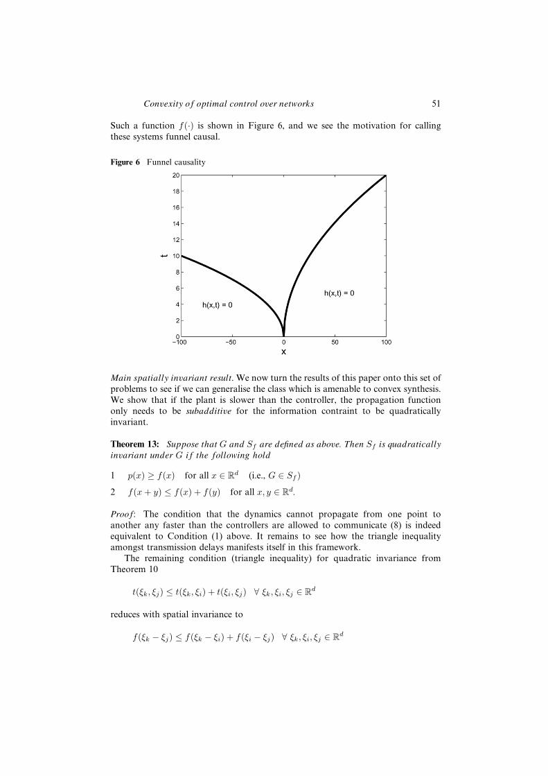
Convexity of optimal control over networks 51
Such a function f(·) is shown in Figure 6, and we see the motivation for callingthese systems funnel causal.
Figure 6 Funnel causality
Main spatially invariant result. We now turn the results of this paper onto this set ofproblems to see if we can generalise the class which is amenable to convex synthesis.We show that if the plant is slower than the controller, the propagation functiononly needs to be subadditive for the information contraint to be quadraticallyinvariant.
Theorem 13: Suppose that G and Sf are defined as above. Then Sf is quadraticallyinvariant under G if the following hold
1 p(x) ≥ f(x) for all x ∈ Rd (i.e., G ∈ Sf )
2 f(x + y) ≤ f(x) + f(y) for all x, y ∈ Rd.
Proof: The condition that the dynamics cannot propagate from one point toanother any faster than the controllers are allowed to communicate (8) is indeedequivalent to Condition (1) above. It remains to see how the triangle inequalityamongst transmission delays manifests itself in this framework.
The remaining condition (triangle inequality) for quadratic invariance fromTheorem 10
t(ξk, ξj) ≤ t(ξk, ξi) + t(ξi, ξj) ∀ ξk, ξi, ξj ∈ Rd
reduces with spatial invariance to
f(ξk − ξj) ≤ f(ξk − ξi) + f(ξi − ξj) ∀ ξk, ξi, ξj ∈ Rd

52 M. Rotkowitz et al.
which, since we can choose x = ξk − ξi, y = ξi − ξj , or conversely, ξj = 0, ξi = y,ξk = x + y, is equivalent to
f(x + y) ≤ f(x) + f(y) ∀ x, y ∈ Rd. �
When d = 1, this includes, but is not limited to, functions which satisfyConditions (2)–(4).
4.3.1 Spatially invariant examples
We now consider the case of one spatial dimension to explore some constraintsets which are not funnel causal but which we now know to also yield convexoptimisation problems.
One type of function which is subadditive but not concave is the step function,f(x) = �x�
B . This is shown is Figure 7, with different values of B for positive andnegative x.
Figure 7 Subadditive step function
Note that it is important that the ceiling function be used rather than the floor, bothto ensure that the function is subadditive (and thus, that the associated informationconstraint is quadratically invariant) as well as to ensure that the function is lowersemicontinuous (and thus, that the epigraph and associated information constraintare closed).
While not explicitly stated, an implicit constraint in Conditions (2)–(4), whencombined with the nonnegativity of f , is that f has to be nonincreasing in R− andnondecreasing in R+. This would typically be desired, as it corresponds to sayingthat information can be transmitted at least as fast over a shorter distance as itcan over a longer distance. However, it is interesting to note that this is no longerrequired either. An example of a subadditive function which violates this assumptionis shown in Figure 8.

Convexity of optimal control over networks 53
Figure 8 Subadditive non-monotonic function
We mostly focused on continuous spatial domains in this paper, but noted that allof the results hold for discrete spatial domains as well. The propagation functionshown in Figure 9,
f(x) =
{0 if x even
1 if x odd
is an example of a propagation function on Z which is indeed subadditive, but whichis not at all concave or monotonic.
Figure 9 Subadditive discrete function
Two other generalisations have been achieved which are more subtle but likelymore important. The first is that Condition (2) is no longer required, and we canhave any f(0) ≥ 0, which could be essential for incorporating computational delay.The second is that, in this framework, it was seamless to consider multiple spatialdimensions d.
5 Conclusions
We have studied the problem of finding optimal controllers subject to delaysbetween different parts of the controller.
We first studied this in the context of control over networks, where multiplesubsystems are subject to constraints on how quickly they can share information.
54 M. Rotkowitz et al.
In Theorem 3 we showed that, presuming the transmission delays satisfy the triangleinequality, if the transmission delay between any pair of subsystems is less than thecorresponding propagation delay, then the information constraint is quadraticallyinvariant. This allows for convex synthesis of the optimal decentralised controllers.
We then studied this problem in the context of spatio-temporal systems, subjectto constraints on how quickly information can be shared between given points.We showed in Theorem 10 that a result analogous to that for networks existsin this context, and that the optimal distributed control problem is convex whenthe transmission delay between any pair of points is less than the correspondingpropagation delay, provided that a similar triangle inequality holds.
We further showed in Theorem 13 that if we apply this result to the specialcase of spatial invariance, it allows us to broadly extend the class of such systemsamenable to convex controller synthesis, to systems in an arbitrary number ofdimensions supported by any subadditive propagation function.
Delay constraints which allow for convex controller synthesis have thus beensimply characterised, unified, and broadly generalised.
Acknowledgements
The authors would like to thank Michael Cantoni for several helpful discussions.
References
Bamieh, B. and Voulgaris, P.G. (2005) ‘A convex characterization of distributed controlproblems in spatially invariant systems with communications constraints’, Systems andControl Letters, Vol. 54, No. 6, pp.575–583.
Papadimitriou, C.H. and Steiglitz, K. (1982) Combinatorial Optimization, Prentice-Hall,Englewood Cliffs, NJ.
Qi, X., Salapaka, M., Voulgaris, P. and Khammash, M. (2004) ‘Structured optimaland robust control with multiple criteria: a convex solution’, IEEE Transactions onAutomatic Control, Vol. 49, No. 10, pp.1623–1640.
Rotkowitz, M. (2006) ‘Parameterization of causal stabilizing controllers over networks withdelays’, Proc. IEEE Global Telecommunications Conference, San Francisco, California,USA, pp.1–5.
Rotkowitz, M. and Lall, S. (2002) ‘Decentralized control information structures preservedunder feedback’, Proc. IEEE Conference on Decision and Control, Las Vegas, Nevada,USA, pp.569–575.
Rotkowitz, M., Cogill, R. and Lall, S. (2005) ‘A simple condition for the convexity of optimalcontrol over networks with delays’, Proc. IEEE Conference on Decision and Control,Seville, Spain, pp.6686–6691.
Rotkowitz, M. and Lall, S. (2006) ‘A characterization of convex problems in decentralizedcontrol’, IEEE Transactions on Automatic Control, Vol. 51, No. 2, pp.274–286.
Voulgaris, P.G. (1999) ‘Control under structural constraints: an input-output approach’,Lecture Notes in Control and Information Sciences, Volume 245, Springer-Verlag,pp.287–305.
Witsenhausen, H.S. (1971) ‘Separation of estimation and control for discrete time systems’,Proceedings of the IEEE, Vol. 59, No. 11, pp.1557–1566.