Embed Size (px)
Citation preview

Cone convexity Convex analysis of convex convex-composite functions Applications References
Convex Convex-Composite FunctionsTim Hoheisel (McGill University, Montreal)
joint work with
James V. Burke (UW, Seattle)
Quang V. Nguyen (McGill, Montreal)
West Coast Optimization Meeting
Vancovuer, September 28, 2019

Cone convexity Convex analysis of convex convex-composite functions Applications References
1. Cone convexity

Cone convexity Convex analysis of convex convex-composite functions Applications References
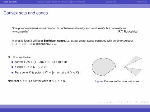
Convex sets and cones
”The great watershed in optimization is not between linearity and nonlinearity, but convexity andnonconvexity.” (R.T. Rockafellar)
In what follows E will be a Euclidean space, i.e. a real-vector space equipped with an inner product〈·, ·〉 : E × E→ R of dimension κ < ∞.
S ⊂ E is said to be
convex if λS + (1 − λ)S ⊂ S (λ ∈ (0, 1));
a cone if λS ⊂ S (λ ≥ 0).
For a cone K its polar is K =v
∣∣∣ 〈v , x〉 ≤ 0 (x ∈ K)
Note that K ⊂ E is a convex cone iff K + K ⊂ K .
0
Figure: Convex set/non-convex cone

Cone convexity Convex analysis of convex convex-composite functions Applications References
Convex sets and cones
”The great watershed in optimization is not between linearity and nonlinearity, but convexity andnonconvexity.” (R.T. Rockafellar)
In what follows E will be a Euclidean space, i.e. a real-vector space equipped with an inner product〈·, ·〉 : E × E→ R of dimension κ < ∞.
S ⊂ E is said to be
convex if λS + (1 − λ)S ⊂ S (λ ∈ (0, 1));
a cone if λS ⊂ S (λ ≥ 0).
For a cone K its polar is K =v
∣∣∣ 〈v , x〉 ≤ 0 (x ∈ K)
Note that K ⊂ E is a convex cone iff K + K ⊂ K .
0
Figure: Convex set/non-convex cone

Cone convexity Convex analysis of convex convex-composite functions Applications References
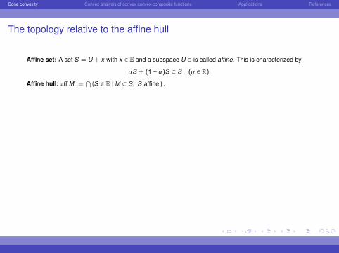
The topology relative to the affine hull
Affine set: A set S = U + x with x ∈ E and a subspace U ⊂ is called affine. This is characterized by
αS + (1 − α)S ⊂ S (α ∈ R).
Affine hull: affM :=⋂S ∈ E | M ⊂ S, S affine .
Relative interior/boundary: C ⊂ E convex.
ri C :=x ∈ C
∣∣∣ ∃ε > 0 : Bε(x) ∩ aff C ⊂ C
(relative interior)x ∈ ri C ⇔ R+(C − x) is a subspace
aff Cri C
C
C aff C ri C
x x x[x, x′] λx + (1 − λ)x′ | λ ∈ R (x, x′)Bε(x) E Bε(x)
Table: Examples for relative interiors
Cone convexity Convex analysis of convex convex-composite functions Applications References
The topology relative to the affine hull
Affine set: A set S = U + x with x ∈ E and a subspace U ⊂ is called affine. This is characterized by
αS + (1 − α)S ⊂ S (α ∈ R).
Affine hull: affM :=⋂S ∈ E | M ⊂ S, S affine .
Relative interior/boundary: C ⊂ E convex.
ri C :=x ∈ C
∣∣∣ ∃ε > 0 : Bε(x) ∩ aff C ⊂ C
(relative interior)x ∈ ri C ⇔ R+(C − x) is a subspace
aff Cri C
C
C aff C ri C
x x x[x, x′] λx + (1 − λ)x′ | λ ∈ R (x, x′)Bε(x) E Bε(x)
Table: Examples for relative interiors

Cone convexity Convex analysis of convex convex-composite functions Applications References
The topology relative to the affine hull
Affine set: A set S = U + x with x ∈ E and a subspace U ⊂ is called affine. This is characterized by
αS + (1 − α)S ⊂ S (α ∈ R).
Affine hull: affM :=⋂S ∈ E | M ⊂ S, S affine .
Relative interior/boundary: C ⊂ E convex.
ri C :=x ∈ C
∣∣∣ ∃ε > 0 : Bε(x) ∩ aff C ⊂ C
(relative interior)
x ∈ ri C ⇔ R+(C − x) is a subspace
aff Cri C
C
C aff C ri C
x x x[x, x′] λx + (1 − λ)x′ | λ ∈ R (x, x′)Bε(x) E Bε(x)
Table: Examples for relative interiors
Cone convexity Convex analysis of convex convex-composite functions Applications References
The topology relative to the affine hull
Affine set: A set S = U + x with x ∈ E and a subspace U ⊂ is called affine. This is characterized by
αS + (1 − α)S ⊂ S (α ∈ R).
Affine hull: affM :=⋂S ∈ E | M ⊂ S, S affine .
Relative interior/boundary: C ⊂ E convex.
ri C :=x ∈ C
∣∣∣ ∃ε > 0 : Bε(x) ∩ aff C ⊂ C
(relative interior)x ∈ ri C ⇔ R+(C − x) is a subspace
aff Cri C
C
C aff C ri C
x x x[x, x′] λx + (1 − λ)x′ | λ ∈ R (x, x′)Bε(x) E Bε(x)
Table: Examples for relative interiors

Cone convexity Convex analysis of convex convex-composite functions Applications References
The topology relative to the affine hull
Affine set: A set S = U + x with x ∈ E and a subspace U ⊂ is called affine. This is characterized by
αS + (1 − α)S ⊂ S (α ∈ R).
Affine hull: affM :=⋂S ∈ E | M ⊂ S, S affine .
Relative interior/boundary: C ⊂ E convex.
ri C :=x ∈ C
∣∣∣ ∃ε > 0 : Bε(x) ∩ aff C ⊂ C
(relative interior)x ∈ ri C ⇔ R+(C − x) is a subspace
aff Cri C
C
C aff C ri C
x x x[x, x′] λx + (1 − λ)x′ | λ ∈ R (x, x′)Bε(x) E Bε(x)
Table: Examples for relative interiors

Cone convexity Convex analysis of convex convex-composite functions Applications References
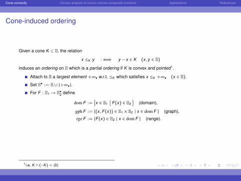
Cone-induced ordering
Given a cone K ⊂ E, the relation
x ≤K y :⇐⇒ y − x ∈ K (x, y ∈ E)
induces an ordering on E which is a partial ordering if K is convex and pointed1.
Attach to E a largest element +∞• w.r.t. ≤K which satisfies x ≤K +∞• (x ∈ E).
Set E• := E ∪ +∞•.
For F : E1 → E•2 define
dom F :=x ∈ E1
∣∣∣ F(x) ∈ E2
(domain),
gph F :=(x,F(x)) ∈ E1 × E2 | x ∈ dom F
(graph),
rge F :=F(x) ∈ E2 | x ∈ dom F
(range).
1 i.e. K ∩ (−K) = 0

Cone convexity Convex analysis of convex convex-composite functions Applications References
Cone-induced ordering
Given a cone K ⊂ E, the relation
x ≤K y :⇐⇒ y − x ∈ K (x, y ∈ E)
induces an ordering on E which is a partial ordering if K is convex and pointed1.
Attach to E a largest element +∞• w.r.t. ≤K which satisfies x ≤K +∞• (x ∈ E).
Set E• := E ∪ +∞•.
For F : E1 → E•2 define
dom F :=x ∈ E1
∣∣∣ F(x) ∈ E2
(domain),
gph F :=(x,F(x)) ∈ E1 × E2 | x ∈ dom F
(graph),
rge F :=F(x) ∈ E2 | x ∈ dom F
(range).
1 i.e. K ∩ (−K) = 0
Cone convexity Convex analysis of convex convex-composite functions Applications References
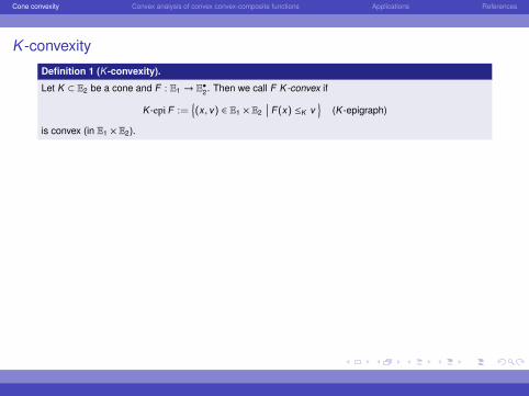
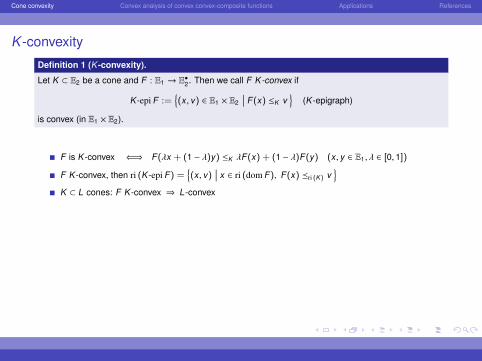
K -convexity
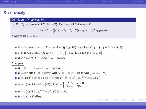
Definition 1 (K -convexity).
Let K ⊂ E2 be a cone and F : E1 → E•2. Then we call F K-convex if
K -epi F :=(x, v) ∈ E1 × E2
∣∣∣ F(x) ≤K v
(K -epigraph)
is convex (in E1 × E2).
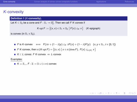
F is K -convex ⇐⇒ F(λx + (1 − λ)y) ≤K λF(x) + (1 − λ)F(y) (x, y ∈ E1, λ ∈ [0, 1])
F K -convex, then ri (K -epi F) =(x, v)
∣∣∣ x ∈ ri (dom F), F(x) ri (K) v
K ⊂ L cones: F K -convex ⇒ L -convex
Examples:
K = R+, F : E→ R ∪ +∞ convex
K = Rm+ and F : E→ (Rm)• with Fi : E→ R ∪ +∞ convex (i = 1, . . . ,m)
K =(x, t) ∈ Rn × R | ‖x‖ ≤ t
and F : Rn → Rn × R, F(x) = (x, ‖x‖)
K = Sn+ and F : Sn → (Sn)•,F(X) =
X−1, X 0,
+∞•, else
K = Sn+ and F : Rm×n → Sn , F(X) = XXT
K arbitrary, F affine.

Cone convexity Convex analysis of convex convex-composite functions Applications References
K -convexity
Definition 1 (K -convexity).
Let K ⊂ E2 be a cone and F : E1 → E•2. Then we call F K-convex if
K -epi F :=(x, v) ∈ E1 × E2
∣∣∣ F(x) ≤K v
(K -epigraph)
is convex (in E1 × E2).
F is K -convex ⇐⇒ F(λx + (1 − λ)y) ≤K λF(x) + (1 − λ)F(y) (x, y ∈ E1, λ ∈ [0, 1])
F K -convex, then ri (K -epi F) =(x, v)
∣∣∣ x ∈ ri (dom F), F(x) ri (K) v
K ⊂ L cones: F K -convex ⇒ L -convex
Examples:
K = R+, F : E→ R ∪ +∞ convex
K = Rm+ and F : E→ (Rm)• with Fi : E→ R ∪ +∞ convex (i = 1, . . . ,m)
K =(x, t) ∈ Rn × R | ‖x‖ ≤ t
and F : Rn → Rn × R, F(x) = (x, ‖x‖)
K = Sn+ and F : Sn → (Sn)•,F(X) =
X−1, X 0,
+∞•, else
K = Sn+ and F : Rm×n → Sn , F(X) = XXT
K arbitrary, F affine.

Cone convexity Convex analysis of convex convex-composite functions Applications References
2. Convex analysis of convexconvex-composite functions
Cone convexity Convex analysis of convex convex-composite functions Applications References
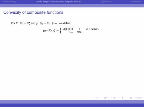
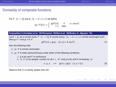
Convexity of composite functions
For F : E1 → E•2 and g : E2 → R ∪ +∞ we define
(g F)(x) :=
g(F(x)) if x ∈ dom F ,
+∞ else.
Proposition 2 (Combari et al. ’95/Pennanen ’99/Bot et al. ’08/Burke, H., Nguyen ’19).
Let K ⊂ E2 be a convex cone, F : E1 → E•2 K-convex and g : E2 → R ∪ +∞ convex and proper such
that rge F ∩ dom g , ∅. Ifg(F(x)) ≤ g(y) ((x, y) ∈ K-epi F) (1)
then the following hold:
a) g F is convex and proper.
b) g F is lower semicontinuous under either of the following conditions:
i) g is lsc and F is continuous;ii) 〈v , F〉 is lsc (proper, convex) for all v ∈ −K and g is lsc and K-increasing, i.e.
x ≤K y =⇒ g(x) ≤ g(y) (x, y ∈ E2). (2)
Observe that (1) is strictly weaker than (2)!

Cone convexity Convex analysis of convex convex-composite functions Applications References
Convexity of composite functions
For F : E1 → E•2 and g : E2 → R ∪ +∞ we define
(g F)(x) :=
g(F(x)) if x ∈ dom F ,
+∞ else.
Proposition 2 (Combari et al. ’95/Pennanen ’99/Bot et al. ’08/Burke, H., Nguyen ’19).
Let K ⊂ E2 be a convex cone, F : E1 → E•2 K-convex and g : E2 → R ∪ +∞ convex and proper such
that rge F ∩ dom g , ∅. Ifg(F(x)) ≤ g(y) ((x, y) ∈ K-epi F) (1)
then the following hold:
a) g F is convex and proper.
b) g F is lower semicontinuous under either of the following conditions:
i) g is lsc and F is continuous;
ii) 〈v , F〉 is lsc (proper, convex) for all v ∈ −K and g is lsc and K-increasing, i.e.
x ≤K y =⇒ g(x) ≤ g(y) (x, y ∈ E2). (2)
Observe that (1) is strictly weaker than (2)!

Cone convexity Convex analysis of convex convex-composite functions Applications References
Convexity of composite functions
For F : E1 → E•2 and g : E2 → R ∪ +∞ we define
(g F)(x) :=
g(F(x)) if x ∈ dom F ,
+∞ else.
Proposition 2 (Combari et al. ’95/Pennanen ’99/Bot et al. ’08/Burke, H., Nguyen ’19).
Let K ⊂ E2 be a convex cone, F : E1 → E•2 K-convex and g : E2 → R ∪ +∞ convex and proper such
that rge F ∩ dom g , ∅. Ifg(F(x)) ≤ g(y) ((x, y) ∈ K-epi F) (1)
then the following hold:
a) g F is convex and proper.
b) g F is lower semicontinuous under either of the following conditions:
i) g is lsc and F is continuous;ii) 〈v , F〉 is lsc (proper, convex) for all v ∈ −K and g is lsc and K-increasing, i.e.
x ≤K y =⇒ g(x) ≤ g(y) (x, y ∈ E2). (2)
Observe that (1) is strictly weaker than (2)!
Cone convexity Convex analysis of convex convex-composite functions Applications References
The main result
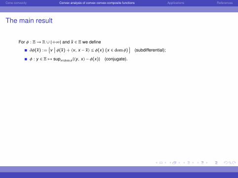
For φ : E→ R ∪ +∞ and x ∈ E we define
∂φ(x) :=v
∣∣∣ φ(x) + 〈v , x − x〉 ≤ φ(x) (x ∈ dom φ)
(subdifferential);
φ : y ∈ E 7→ supx∈dom φ〈y, x〉 − φ(x) (conjugate).
Theorem 3 (Burke,H., Nguyen ’19).
Let K ⊂ E2 be a closed, convex cone, F : E1 → E•2 K-convex and f : E1 → R ∪ +∞, g : E2 → R ∪ +∞
proper, convex such thatg(F(x)) ≤ g(y) ((x, y) ∈ K-epi F).
andF(ri (dom f) ∩ ri (dom F)) ∩ ri (dom g − K) , ∅. (3)
Then (f + g F is convex and) the following hold:
a) (f + g F)∗(p) = minv∈−K ,y∈E1
g∗(v) + f∗(y) + 〈v , F〉∗ (p − y);
b) ∂(f + g F)(x) = ∂f(x) +⋃
v∈∂g(F(x)) ∂ 〈v , F〉 (x) (x ∈ dom f ∩ dom g F).

Cone convexity Convex analysis of convex convex-composite functions Applications References
The main result
For φ : E→ R ∪ +∞ and x ∈ E we define
∂φ(x) :=v
∣∣∣ φ(x) + 〈v , x − x〉 ≤ φ(x) (x ∈ dom φ)
(subdifferential);
φ : y ∈ E 7→ supx∈dom φ〈y, x〉 − φ(x) (conjugate).
Theorem 3 (Burke,H., Nguyen ’19).
Let K ⊂ E2 be a closed, convex cone, F : E1 → E•2 K-convex and f : E1 → R ∪ +∞, g : E2 → R ∪ +∞
proper, convex such thatg(F(x)) ≤ g(y) ((x, y) ∈ K-epi F).
andF(ri (dom f) ∩ ri (dom F)) ∩ ri (dom g − K) , ∅. (3)
Then (f + g F is convex and) the following hold:
a) (f + g F)∗(p) = minv∈−K ,y∈E1
g∗(v) + f∗(y) + 〈v , F〉∗ (p − y);
b) ∂(f + g F)(x) = ∂f(x) +⋃
v∈∂g(F(x)) ∂ 〈v , F〉 (x) (x ∈ dom f ∩ dom g F).

Cone convexity Convex analysis of convex convex-composite functions Applications References
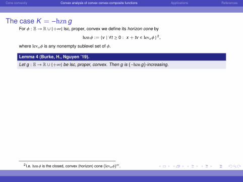
The case K = −hzn gFor φ : E→ R ∪ +∞ lsc, proper, convex we define its horizon cone by
hzn φ := v | ∀t ≥ 0 : x + tv ∈ levαφ 2,
where levαφ is any nonempty sublevel set of φ.
Lemma 4 (Burke, H., Nguyen ’19).
Let g : E→ R ∪ +∞ be lsc, proper, convex. Then g is (−hzn g)-increasing.
Corollary 5 (Burke, H., Nguyen ’19).
g : E→ R ∪ +∞ be lsc, proper, convex and let F : E1 → E•2 be (−hzn g)-convex such that
F(ri (dom F)) ∩ ri (dom g) , ∅.
Then(g F)∗(p) = min
v∈E2g∗(v) + 〈v , F〉∗ (p)
and∂(g F)(x) =
⋃v∈∂g(F(x))
∂ 〈v , F〉 (x) (x ∈ dom g F).
Proof.K = −hzn g.
2 I.e. hzn φ is the closed, convex (horizon) cone (levαφ)∞ .
Cone convexity Convex analysis of convex convex-composite functions Applications References
The case K = −hzn gFor φ : E→ R ∪ +∞ lsc, proper, convex we define its horizon cone by
hzn φ := v | ∀t ≥ 0 : x + tv ∈ levαφ 2,
where levαφ is any nonempty sublevel set of φ.
Lemma 4 (Burke, H., Nguyen ’19).
Let g : E→ R ∪ +∞ be lsc, proper, convex. Then g is (−hzn g)-increasing.
Corollary 5 (Burke, H., Nguyen ’19).
g : E→ R ∪ +∞ be lsc, proper, convex and let F : E1 → E•2 be (−hzn g)-convex such that
F(ri (dom F)) ∩ ri (dom g) , ∅.
Then(g F)∗(p) = min
v∈E2g∗(v) + 〈v , F〉∗ (p)
and∂(g F)(x) =
⋃v∈∂g(F(x))
∂ 〈v , F〉 (x) (x ∈ dom g F).
Proof.K = −hzn g.
2 I.e. hzn φ is the closed, convex (horizon) cone (levαφ)∞ .

Cone convexity Convex analysis of convex convex-composite functions Applications References
Component-wise convex functions
Corollary 6.
Let g : Rm → R ∪ +∞ be proper, convex and Rm+-increasing, F : E→ (Rm)• with Fi (i = 1, . . . ,m)
proper, convex such that
F
m⋂i
ri (dom Fi)
∩ ri (dom g) , ∅.
Then
(g F)∗(p) = minv≥0
g∗(v) +
m∑i=1
viFi
∗ (p)
and
∂(g F)(x) =⋃
v∈∂g(F(x))
m∑i=1
vi∂Fi(x) (x ∈ dom g F).
Proof.Use K = Rm
+ and observe that F is K -convex.
Cone convexity Convex analysis of convex convex-composite functions Applications References
3. Applications

Cone convexity Convex analysis of convex convex-composite functions Applications References
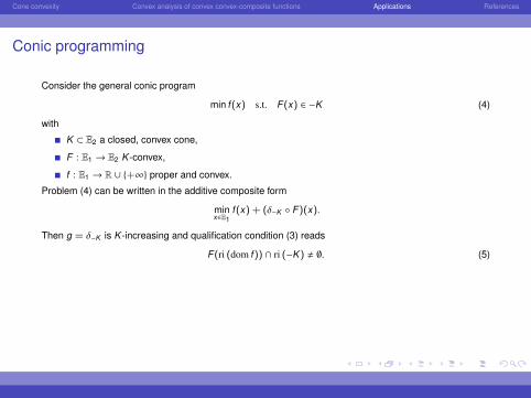
Conic programming
Consider the general conic program
min f(x) s.t. F(x) ∈ −K (4)
with
K ⊂ E2 a closed, convex cone,
F : E1 → E2 K -convex,
f : E1 → R ∪ +∞ proper and convex.
Problem (4) can be written in the additive composite form
minx∈E1
f(x) + (δ−K F)(x).
Then g = δ−K is K -increasing and qualification condition (3) reads
F(ri (dom f)) ∩ ri (−K) , ∅. (5)
Under (5) we haveinf
x∈E1f(x) + (δ−K F)(x) = max
v∈−K−f∗(y) − (δ−K F)∗(−y)
= maxv∈−K
infx∈E1
f(x) +⟨v , F(x)
⟩.

Cone convexity Convex analysis of convex convex-composite functions Applications References
Conic programming
Consider the general conic program
min f(x) s.t. F(x) ∈ −K (4)
with
K ⊂ E2 a closed, convex cone,
F : E1 → E2 K -convex,
f : E1 → R ∪ +∞ proper and convex.
Problem (4) can be written in the additive composite form
minx∈E1
f(x) + (δ−K F)(x).
Then g = δ−K is K -increasing and qualification condition (3) reads
F(ri (dom f)) ∩ ri (−K) , ∅. (5)
Under (5) we haveinf
x∈E1f(x) + (δ−K F)(x) = max
v∈−K−f∗(y) − (δ−K F)∗(−y)
= maxv∈−K
infx∈E1
f(x) +⟨v , F(x)
⟩.

Cone convexity Convex analysis of convex convex-composite functions Applications References
Conic programming II
Consider againmin f(x) s.t. F(x) ∈ −K . (6)
Observe that∂δ−K (y) =
v
∣∣∣ 〈v , y − y〉 ≥ 0 (y ∈ K)
=: N−K (y) (y ∈ −K).
Theorem 7 (Pennanen ’99/Burke, H.,Nguyen ’19).
Let f ∈ Γ(E1), K ⊂ E2 a closed, convex cone, and let F : E1 → E2 be K-convex. Then the condition
0 ∈ ∂f(x) +⋃
v∈N−K (F(x))
∂ 〈v , F〉 (x) (7)
is sufficient for x to be a minimizer of (6). Under the condition F(ri (dom f)) ∩ ri (−K) , ∅ it is alsonecessary.
Corollary 8.
Let f : E1 → R be differentiable and convex, K ⊂ E2 a closed, convex cone, and let F : E1 → E2 bedifferentiable and K-convex. Then the condition
− ∇f(x) ∈ F ′(x)∗N−K (F(x)) (8)
is sufficient for x to be a minimizer of (6). Under the condition rge F ∩ ri (−K) , ∅ it is also necessary.

Cone convexity Convex analysis of convex convex-composite functions Applications References
Variational Gram functionsGiven M ⊂ Sn
+ closed and convex, the associated variational Gram function (VGF) is given by
ΩM : Rn×m → R ∪ +∞, ΩM(X) =12σM(XXT ) := sup
V∈Mtr (VXXT ).
Then
F : X ∈ Rn×m 7→ XXT is Sn+-convex;
σK-epi F (X ,−V) =
12 tr
(XT V†X
), if rge X ⊂ rge V , V 0,
+∞, else(matrix-fractional function);
σM is Sn+-increasing;
M is bounded if and only if rge F ∩ ri (domσM) , ∅.
Proposition 9 (Jalali et al. ’17/Burke, Gao, H.’ 18/Burke, H.,Nguyen ’19).
Let M ⊂ Sn+ be nonempty, convex and compact. Then Ω∗M is finite-valued and given by
Ω∗M(X) =12
minV∈M
tr (XT V†X)
∣∣∣ rge X ⊂ rge V.
and
∂ΩM(X) =
VX
∣∣∣∣∣∣ V ∈ arg maxM
⟨XXT , ·
⟩ is compact for all X.

Cone convexity Convex analysis of convex convex-composite functions Applications References
Extending the matrix-fractional function
Consider the Euclidean space G := Cn×m × Hn equipped with the inner product
〈·, ·〉 : ((X ,U), (Y ,V)) ∈ G × G 7→ Re tr (Y∗X) + Re tr (VU).
Define the mapping F : G→ (Hn)• by
F(X ,V) :=
X∗V†X if rge X ⊂ rge V ,
+∞•, else, (9)
where X∗ is the adjoint of X and V† is the Moore-Penrose pseudoinverse of V .
Proposition 10 (Burke, H., Nguyen, ’11).
Let F : G→ (Hn)• be given by (9) and define γ : G→ R ∪ +∞ by
γ(X ,V) :=
12 tr (F(X ,V)) , if rge X ⊂ rge V , V 0
+∞, else.
Then γ is lsc, proper, and convex, hence a support function.

Cone convexity Convex analysis of convex convex-composite functions Applications References
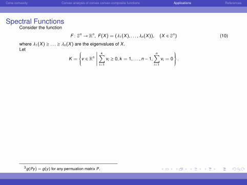
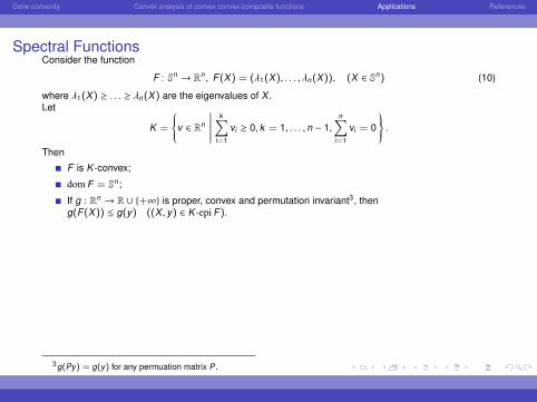
Spectral FunctionsConsider the function
F : Sn → Rn , F(X) = (λ1(X), . . . , λn(X)), (X ∈ Sn) (10)
where λ1(X) ≥ . . . ≥ λn(X) are the eigenvalues of X .
Let
K =
v ∈ Rn
∣∣∣∣∣∣∣k∑
i=1
vi ≥ 0, k = 1, . . . , n − 1,n∑
i=1
vi = 0
.Then
F is K -convex;
dom F = Sn ;
If g : Rn → R ∪ +∞ is proper, convex and permutation invariant3, theng(F(X)) ≤ g(y) ((X , y) ∈ K -epi F).
Proposition 11 (Lewis ’95/Burke, H., Nguyen ’19).
Let g be proper, convex and permutation invariant and let F : Sn → Rn be given by (10). Then thefollowing hold:
a) g F is convex and (g F)∗ = g∗ F .
b) For all X ∈ F−1(dom g) we have that
∂(g F)(X) =⋃
v∈∂g(λ(X))
convU∗diag(v)U
∣∣∣ U∗XU = diag(F(X)), U∗U = In.
3g(Py) = g(y) for any permuation matrix P.
Cone convexity Convex analysis of convex convex-composite functions Applications References
Spectral FunctionsConsider the function
F : Sn → Rn , F(X) = (λ1(X), . . . , λn(X)), (X ∈ Sn) (10)
where λ1(X) ≥ . . . ≥ λn(X) are the eigenvalues of X .Let
K =
v ∈ Rn
∣∣∣∣∣∣∣k∑
i=1
vi ≥ 0, k = 1, . . . , n − 1,n∑
i=1
vi = 0
.
Then
F is K -convex;
dom F = Sn ;
If g : Rn → R ∪ +∞ is proper, convex and permutation invariant3, theng(F(X)) ≤ g(y) ((X , y) ∈ K -epi F).
Proposition 11 (Lewis ’95/Burke, H., Nguyen ’19).
Let g be proper, convex and permutation invariant and let F : Sn → Rn be given by (10). Then thefollowing hold:
a) g F is convex and (g F)∗ = g∗ F .
b) For all X ∈ F−1(dom g) we have that
∂(g F)(X) =⋃
v∈∂g(λ(X))
convU∗diag(v)U
∣∣∣ U∗XU = diag(F(X)), U∗U = In.
3g(Py) = g(y) for any permuation matrix P.

Cone convexity Convex analysis of convex convex-composite functions Applications References
Spectral FunctionsConsider the function
F : Sn → Rn , F(X) = (λ1(X), . . . , λn(X)), (X ∈ Sn) (10)
where λ1(X) ≥ . . . ≥ λn(X) are the eigenvalues of X .Let
K =
v ∈ Rn
∣∣∣∣∣∣∣k∑
i=1
vi ≥ 0, k = 1, . . . , n − 1,n∑
i=1
vi = 0
.Then
F is K -convex;
dom F = Sn ;
If g : Rn → R ∪ +∞ is proper, convex and permutation invariant3, theng(F(X)) ≤ g(y) ((X , y) ∈ K -epi F).
Proposition 11 (Lewis ’95/Burke, H., Nguyen ’19).
Let g be proper, convex and permutation invariant and let F : Sn → Rn be given by (10). Then thefollowing hold:
a) g F is convex and (g F)∗ = g∗ F .
b) For all X ∈ F−1(dom g) we have that
∂(g F)(X) =⋃
v∈∂g(λ(X))
convU∗diag(v)U
∣∣∣ U∗XU = diag(F(X)), U∗U = In.
3g(Py) = g(y) for any permuation matrix P.

Cone convexity Convex analysis of convex convex-composite functions Applications References
4. References

Cone convexity Convex analysis of convex convex-composite functions Applications References
J. M. Borwein: Optimization with respect to Partial Orderings. Ph.D. Thesis, University of Oxford,1974.
R.I. Bot, S.-M. Grad, and G. Wanka: A new constraint qualification for the formula of thesubdifferential of composed convex functions in infinite dimensional spaces. MathematischeNachrichten 281, 2008, pp. 1088–1107.
R.I. Bot, S.-M. Grad, and G. Wanka: Generalized Moreau-Rockafellar results for composed convexfunctions. Optimization 58(7), 2009, pp. 917–933.
J. V. Burke and T. Hoheisel: Matrix support functionals for inverse problems, regularization, andlearning. SIAM Journal on Optimization 25, 2015, pp. 1135–1159.
J. V. Burke, Y. Gao and T. Hoheisel: Convex Geometry of the Generalized Matrix-FractionalFunction. SIAM Journal on Optimization 28, 2018, pp. 2189–2200.
J. V. Burke, Y. Gao, and T. Hoheisel: Variational properties of matrix functions via the generalizedmatrix-fractional function. SIAM Journal on Optimization, to appear.
J. V. Burke, T. Hoheisel, and Q.V. Nguyen:A study of convex convex-composite functions via infimalconvolution with applications. arXiv:1907.08318.
A. Jalali, M. Fazel, and L. Xiao: Variational Gram Functions: Convex Analysis and Optimization.SIAM Journal on Optimization 27(4), 2017, pp. 2634–2661.
J.-B. Hiriart-Urruty: A Note on the Legendre-Fenchel Transform of Convex Composite Functions.in Nonsmooth Mechanics and Analysis. Eds. P. Alart, O. Maisonneuve, and R. T. Rockafellar,Springer, 2006, pp. 35–46.
Cone convexity Convex analysis of convex convex-composite functions Applications References
A.G. Kusraev and S.S. Kutateladze: Subdifferentials: theory and applications. Mathematics and itsApplications, 323. Kluwer Academic Publishers Group, Dordrecht, 1995.
A.S. Lewis: The convex analysis of unitarily invariant matrix functions. Journal of Convex Analysis2(1–2), 1995, pp. 173–183.
A.S. Lewis:Convex analysis on the hermitian Matrices SIAM Journal on Optimimization 6(1), 1996,pp. 164–177.
T. Pennanen: Graph-Convex Mappings and K-Convex Functions. Journal of Convex Analysis 6(2),1999, pp. 235–266.
R.T. Rockafellar: Convex Analysis. Princeton Mathematical Series, No. 28. Princeton UniversityPress, Princeton, N.J. 1970.
R.T. Rockafellar and R.J.-B. Wets: Variational Analysis. Grundlehren der MathematischenWissenschaften, Vol. 317, Springer-Verlag, Berlin, 1998.


![The Cyclic Block Conditional Gradient Method for Convex ...[22] provides an asymptotic analysis of exact coordinate minimization for composite strongly convex problems. In [6], a global](https://img.dokumen.tips/doc/110x75/5eb4b293d461183e56529aba/the-cyclic-block-conditional-gradient-method-for-convex-22-provides-an-asymptotic.jpg)