1

Converting Washington Lignocellulosic Rich Urban Waste to Ethanol1,2

Rick Gustafson (

pulp@u.washington.edu), College of Forest Resources3

Renata Bura (

renatab@u.washington.edu), College of Forest Resources Joyce Cooper (cooperjs@u.washington.edu), Department of Mechanical Engineering Ryan McMahon (mcmahr@u.washington.edu ) College of Forest Resources Elliott Schmitt (schmie11@u.washington.edu), Department of Mechanical Engineering Azra Vajzovic (azra@u.washington.edu) College of Forest Resources

University of Washington, Seattle, WA 98195

1 The Washington State Department of Ecology provided funding for this project through the Beyond Waste Organics Waste to Resources (OWR) project. These funds were provided in the 2007-2009 Washington State budget from the Waste Reduction Recycling and Litter Control Account. OWR project goals and objectives were developed by the Beyond Waste Organics team, and were approved by the Solid Waste and Financial Assistance Program. Funding was from the Waste Reduction Recycling and Litter Control Account. OWR project goals and objectives were developed by the Beyond Waste Organics team, and were approved by the Solid Waste and Financial Assistance Program. 2 This report is available on the Department of Ecology’s website at www.ecy.wa.gov/beyondwaste/organics. The reader may be interested in the other project reports supported by Organic Waste to Resources and Waste to Fuel Technology funding sponsored by Ecology. These are also available on the “organics” link. The Washington State University Extension Energy Program will make this report accessible in its broader library of bioenergy information on www.pacificbiomass.org. The online Denman Forestry Issues series http://www.uwtv.org/programs/displayseries.aspx?fID=558 is an excellent source of forest ecology, assessment, and climate information. 3 Please send inquiries to Rick Gustafson, School of Forest Resources, Box 352100, Seattle, WA 98195

Converting Washington Lignocellulosic Rich Urban Waste to Ethanol

Ecology Publication Number 09-07-060

To ask about the availability of this document in a format for the visually impaired, call the Solid Waste and Financial Assistance Program at 360-407-6900. Persons with hearing loss can call 711 for Washington Relay Service. Persons with a speech disability can call 877-833-6341.

2

Table of Contents

EXECUTIVE SUMMARY ................................................................................................ 4

CONVERTING WASHINGTON LIGNOCELLULOSIC RICH URBAN WASTE TO ETHANOL: PART 1, PROCESS DEVELOPMENT ............................................................. 6

Introduction ................................................................................................................................................................ 6

Background and methods ...................................................................................................................................... 6 Pretreatment-background ......................................................................................................................... 6 Pretreatment-Methods ............................................................................................................................... 7 Enzymatic hydrolysis-Background ........................................................................................................ 8 Enzymatic hydrolysis-Methods ............................................................................................................... 9 Fermentation-Background ....................................................................................................................... 9 Fermentation-Methods ............................................................................................................................ 10 Methods for analytic procedures .......................................................................................................... 11

Results and Discussion ........................................................................................................................................ 12 Lignocellulosic rich urban waste composition ................................................................................. 12 Monomeric and oligomeric sugars ...................................................................................................... 12 Recovery of sugars after pretreatment ............................................................................................... 13 Enzymatic hydrolysis............................................................................................................................... 13 Fermentation .............................................................................................................................................. 14

Conclusion ............................................................................................................................................................... 15

Tables and Figures ................................................................................................................................................. 16

References ................................................................................................................................................................ 18

CONVERTING WASHINGTON LIGNOCELLULOSIC RICH URBAN WASTE TO ETHANOL: PART 2, PROCESS MODELING AND LIFE CYCLE ASSESSMENT ............... 22

Introduction .............................................................................................................................................................. 22 ISO Standards ............................................................................................................................................ 22

Goal & Scope ........................................................................................................................................................... 22 Functional Unit .......................................................................................................................................... 24 System Boundaries .................................................................................................................................. 24

Life Cycle Inventory ............................................................................................................................................... 25 Collection Module ..................................................................................................................................... 25

Commercial Collection ................................................................................................................................ 26 Self-haul ........................................................................................................................................................... 29

Intermediate Waste Processing ............................................................................................................ 30 Transfer Stations ........................................................................................................................................... 30 Intermodal rail-yard ...................................................................................................................................... 31 Material Recovery Facility ........................................................................................................................... 32

Landfill ......................................................................................................................................................... 34 Daily Operations at Landfill ........................................................................................................................ 34

3

Landfill Gas Collection and Electricity Production .............................................................................. 35 Leachate Generation and Waste Water Treatment ............................................................................... 37

Recycling Mixed Waste Paper ............................................................................................................... 38 Recycled Pulp Operations .......................................................................................................................... 38 Virgin Pulp Production ................................................................................................................................ 39

Composting ................................................................................................................................................ 39 Windrow Turning Facility ............................................................................................................................ 39 Commercial Fertilizer Production ............................................................................................................. 41

Biorefinery .................................................................................................................................................. 41 Feedstock Handling & Pretreatment ........................................................................................................ 43 ASPEN Model Development ....................................................................................................................... 45 U.S. Corn Ethanol Production .................................................................................................................... 47

Chemicals Production ............................................................................................................................. 47 Sulfuric Acid Production ............................................................................................................................. 47 Lime Production ............................................................................................................................................ 47 Ammonia Phosphate Production .............................................................................................................. 48 Enzyme Production ...................................................................................................................................... 48 Corn Steep Liquor Production ................................................................................................................... 48

Energy & Fuel Production ...................................................................................................................... 48 GREET Data .................................................................................................................................................... 48

Life Cycle Impact Assessment ............................................................................................................................ 48

Process Economics ............................................................................................................................................... 57 Methods ....................................................................................................................................................... 57

Total Project Investment ............................................................................................................................. 57 Variable Operating Costs ............................................................................................................................ 57 Fixed Operating Costs ................................................................................................................................. 57 Discounted Cash Flow Analysis ............................................................................................................... 57

Results ......................................................................................................................................................... 58 Discussion .................................................................................................................................................. 60

Recommendations & Conclusion ....................................................................................................................... 60

References ................................................................................................................................................................ 62

Appendix A: LCI data results ............................................................................................................................... 65

Appendix B: GREET LCI Data .............................................................................................................................. 68

Appendix C: Equipment Emission Factors ...................................................................................................... 73

4

Executive Summary

The objective of this research was to investigate the potential of producing ethanol from municipal waste in Washington State. The approach to the research was to divide the municipal waste into three primary streams and then investigate the potential of converting each into ethanol. This division was made to provide a more fundamental understanding of the issues associated with conversion for each of the major streams. The three primary streams were mixed waste paper, yard waste, and municipal solid waste4

Process Development:

. For each stream, an experimental study was done to investigate conversion of the biomass into ethanol using bioconversion processes. This experimental work was then accompanied by a Life Cycle Assessment (LCA) to determine the overall environmental impact of the proposed processes. ASPEN models of biorefineries were developed to provide process data for the LCA. An assessment of economic viability was also performed based on the ASPEN models. Following are the main conclusions of the study.

· The paper, yard and municipal solid waste are sugar rich lignocellulosic feedstocks.

· Dilute acid hydrolysis is an effective pretreatment method for paper and municipal solid waste. Steam pretreatment (210°C, 10 min and 3% SO2) is a good pretreatment method for fractionation of yard waste into hemicellulose, cellulose and lignin rich fractions.

· The water insoluble fractions of municipal solid and paper waste are easily hydrolysable by enzymes. Almost theoretical cellulose to glucose conversion was achieved.

· The water insoluble fraction of yard waste is difficult to hydrolyze by enzymes (41% cellulose to glucose conversion). However, the low cellulose to glucose conversion yields were expected since the biomass was composed of mixture of branches, wood chips, bark, and needles.

· The results obtained during this study demonstrate that the UW developed PTD3 yeast was able to very efficiently convert yard waste hydrolysate to ethanol with a yield 100% of theoretical during the fermentation process. Pretreated and hydrolyzed sugars of municipal solid, paper and yard waste are readily fermentable by yeast. High ethanol yields were obtained (100% of theoretical). Overall ethanol yields of 105 gallons/ton, 90 gallons/ton, and 55 gallons/ton are estimated for municipal solid waste, paper waste, and yard waste respectively. Typical yields for cellulosic ethanol produced using hydrolysis and fermentation are on the order of 80 gallons per ton but can vary widely depending on biomass feedstock. (See the Theoretical Ethanol Yield Calculator for details - http://www1.eere.energy.gov/biomass/ethanol_yield_calculator.html )

4 For this research municipal solid waste (MSW) refers to the organic fraction of residential garbage found in King County. It is similar in composition to garbage where the metal, textiles, and plastics have been removed. The composition of the material is provided in the main body the report.

5

Life Cycle Assessment: · Municipal solid waste seems to offer the greatest potential as both a waste

management strategy and for bio-fuel production. With over 4 million metric tons of MSW generated in 2007, there is enough lignocellulosic material available to meet the demands of a large capacity biorefinery within the State.

· The greatest contributor to ethanol production environmental flows is chemicals production, specifically lime production. On the other hand, avoidance of dry-mill corn ethanol greatly reduces the environmental flows for ethanol production.

· Landfilled waste offers the least benefit overall, even with production of electricity and avoidance of Washington electric grid. This is related to the fact that the Washington electric grid is largely dominated by clean hydropower and offers little benefit from avoidance.

The process economic analysis suggests that the conversion of MSW to ethanol is economically viable. The ease of conversion and good process yields for this raw material results in reasonable minimum ethanol selling prices even when using conventional Brewer’s yeast as a fermentation organism. It should be noted that we did not evaluate the potential for production of high value co-products in this investigation. The process economics could be considerably more favorable with the addition of these product streams.

In general it appears that conversion of material currently sent to landfills would be an excellent feedstock for ethanol production. This material is rich in carbohydrates, can be readily converted to ethanol, and the life cycle impact is reduced by avoiding land filling.

The results of this research are preliminary, however. More work is required to optimize the conversions of each primary stream, especially the recalcitrant yard waste, and conversion research on actual municipal solid waste streams needs to be carried out. The LCA work needs to be expanded to consider all environmental impacts, especially those associated with water usage and aqueous effluents. A more detailed economic analysis is needed to thoroughly assess economic viability. The excellent results obtained from this preliminary study suggest that these more in-depth investigations would be successful and would provide data required to construct a commercial facility.

6

Converting Washington Lignocellulosic Rich Urban Waste to Ethanol: Part 1, Process Development

Introduction During the past few decades, global warming has emerged as a major political and scientific issue. This is due primarily to increased emissions of greenhouse gases formed by burning fossil fuels, concurrent with increased energy consumption (Dickerson and Johnson, 2004; Sun and Cheng, 2002). Various studies have shown that ethanol or ethanol-blended transportation fuels produce less harmful emissions, while the production of ethanol from biomass has the advantage of displacing transportation fuels derived from oil with a fuel obtained from a renewable resource (Bergeron, 1996; Galbe and Zacchi, 2002; Tyson, 1993; von Sivers and Zacchi, 1995). In addition to environmental reasons, other motivations, such as fossil fuel exhaustion, geopolitical concerns about reliance on foreign fuel supplies, and the ease of adaptation to a carbon-based fuel are some of the factors influencing the emergence of ethanol as a viable fuel supplement and/or alternative to gasoline. Although the major ethanol producers currently use either sugar cane (Brazil) or corn (North America) as the substrate for the “sugar to ethanol process”, various lignocellulosic biomass feedstocks, including: agricultural residues, wood residues, food-processing waste, municipal solid wastes, herbaceous energy crops and pulp and paper industry wastes have the potential to serve as low-cost, abundant feedstocks for the production of fuel ethanol (Wiselogel, et al., 1996). Approximately four million tons of municipal solid waste is available in Washington State for use a biofuel feedstock (Frear, et al., 2005). Since much of this material is currently sent to landfills, composted, or is recycled, the research proposed here will develop and assess an alternative management system. Specifically, the objective of the proposed research is to evaluate the potential for using urban lignocellulosic waste to produce bioethanol on the basis of potential economic, environmental, and economic development benefits for Washington State. Municipal solid waste, due to its chemical and structural properties, was evaluated as a potential technically viable feedstock that might be used to demonstrate the effectiveness of a biomass to ethanol bioconversion process. For the past year, the Bioenergy group at the College of Forest Resources at the University of Washington has focused on studying the bioconversion process of lignocellulosic rich urban waste to ethanol. The proposed research had one main task: to develop an optimized process for converting lignocellulosic rich urban waste to ethanol. In this study the lignocellulosic rich urban waste was divided into three streams: municipal solid waste, paper waste and yard waste.

Background and methods Pretreatment-background Various pretreatment options have been used to fractionate, solubilise, hydrolyse, and separate cellulose, hemicellulose and lignin moieties. These different processes usually

7

exploit a combination of chemical, physical and mechanical treatments that serve to render the lignocellulosics more receptive to subsequent enzymatic hydrolysis. The physical pretreatment techniques do not involve chemical application, and typical examples are milling, irradiation, steam explosion, and hydrothermolysis (high-temperature cooking) (Hsu, 1996). Chemical pretreatment techniques have received the most attention by far among all the categories of pretreatment methods and typical examples include dilute acid, alkali, solvent, ammonia, SO2, CO2, other chemicals, steam explosion and pH-controlled hydrothermolysis (McMillan, 1993). Steam pretreatment is the treatment of biomass with stream at high temperature and pressure for the certain period of time followed by sudden decompression. Previous work has shown that SO2-catalysed steam explosion can successfully pretreat softwood (Boussaid, et al., 2000; Carrasco, 1992; Clark, et al., 1989; Clark and Mackie, 1987; Schwald, et al., 1989b; Söderström, et al., 2002; Stenberg, et al., 1998; Tengborg, et al., 1998) and hardwood residues (Eklund, et al., 1995; Mackie, et al., 1985; Schwald, et al., 1989a) as part of the overall bioconversion process. In addition, steam explosion is recognized as one the most cost effective pretreatments for lignocellulosic residues prior to enzymatic saccharification (Clark and Mackie, 1987). The impregnation of SO2 allows lower temperatures and shorter reaction times, and thereby reduces the formation of degradation products (Excoffier, et al., 1991). The use of SO2 as a catalyst results in improved enzymatic accessibility to cellulose and enhanced recovery of the hemicellulose-derived sugars (Boussaid, et al., 1999; Boussaid, et al., 2000). It was reported that more than 75% of the original hemicellulose-derived sugars can be recovered in the water soluble fraction after steam explosion of Douglas-fir (Pseudotsuga menziesii) wood chips at relatively mild conditions (Boussaid, et al., 2000). It has been shown previously that adding SO2 prior to steam explosion enhanced the carbohydrate hydrolysis rate, while reducing the degree of polymerization of the oligomers and increasing the proportion of monomers in the water soluble stream (Clark, et al., 1989). In addition, a combination of steam explosion with acid hydrolysis increases pore volume and enzyme accessibility, reduces particle size (Boussaid, et al., 2000) and increases the available surface area (Michalowicz, et al., 1991). In this study steam explosion was employed to pretreate the yard waste and diluted acid pretreatment was employed to pretreat municipal solid and paper waste.

Pretreatment-Methods The yard waste, mixture of hardwood and softwood with branches, bark, needles (60.0 % moisture content) was obtained from the University of Washington waste facility and stored at 4°C until use. Yard waste was composed of shrubbery cuttings, leaves, needles, tree limbs, and other materials was pretreated by soaking in water overnight prior to SO2-catalysed steam explosion. Prior to SO2-catalysed steam explosion, the biomass was kept a sealed plastic container to ensure uniform moisture content. Samples of 300g oven-dried weight (ODW) were impregnated overnight with anhydrous SO2 in plastic bags. The samples were then loaded, in 50g batches, into a preheated 2L steam gun in Gresham, Oregon and exploded at temperature of 210°C; time 10 minutes and 3% (w/w) SO2 concentration The recovered slurries were separated by filtration and kept at 4°C until use.

8

The paper waste was obtained from the Tacoma recycling facility owned by Weyerhaeuser and consisted of the lowest grade paper waste. The municipal solid waste was prepared in the lab due to the safety issues. It’s composition was based on the organic fraction of residential waste in King County and is similar to that refuse stream where the metal, textiles, and plastics have been removed. Specifically the composition was 50% food waste and 50% of mixed waste papers including clean hygiene products which also contained incidental plastics. The food waste included banana peels, cereal, coffee grinds, canned corn, and tomato juice. The paper waste and municipal solid waste were pretreated by diluted sulfuric acid at 60°C for 6 hours. Then the slurry was recovered, separated by filtration and kept at 4°C until use.

Enzymatic hydrolysis-Background The pretreatment processes are designed only to initiate the breakdown of the biomass structure and partially hydrolyze the carbohydrate polymers, making them accessible to enzymatic attack. Hydrolysis of cellulose to glucose can be achieved using either inorganic acids or cellulolytic enzymes. Chemical hydrolysis of biomass is relatively efficient and inexpensive, however, it generates fermentation inhibitors (Leathers, 2003). On the other hand, enzymatic hydrolysis, despite its relatively slow rate, is a biocompatible and environmentally friendly option (as it avoids the use of corrosive chemicals). Cellulases, perform a crucial task during saccharification by catalyzing the hydrolysis of cellulose to soluble and fermentable carbohydrates. They are synthesized mainly by fungi and bacteria and are produced both aerobically and anaerobically. The aerobic mesophilic fungus Trichoderma reesei and its mutants have been the most intensively studied source of cellulases (Philippidis, 1996). The enzyme system for the conversion of cellulose to glucose generally comprises three distinct classes of enzyme (Lynd, et al., 2002):

· endoglucanases or 1,4-β-D-glucan-4-glucanohydrolases (EC 3.2.1.4), · exoglucanases, including 1,4-β-D-glucan glucanohydrolases (also known as

cellodextrinases) (EC 3.2.1.74) and 1,4-β-D-glucan cellobiohydrolases (also known as cellobiohydrolases) (EC 3.2.1.91), and

· β-glucosidases or β-glucoside glucohydrolases (EC 3.2.1.21). Endoglucanases cut at random, at internal amorphous sites in the cellulose polysaccharide chain, and generate oligosaccharides of varying lengths and consequently new chain ends (Mansfield, et al., 1999). Exoglucanases act on the reducing and nonreducing ends of cellulose polysaccharide chains, liberating either glucose (glucanohydrolases) or cellobiose (cellobiohydrolase) as major products (Mansfield, et al., 1999). Exoglucanases can also act on microcrystalline cellulose, presumably peeling cellulose chains from the microcrystalline structure (Lynd, et al., 2002). β-Glucosidases hydrolyse soluble cellodextrins and cellobiose to glucose (Bothast and Saha, 1997). Cellulase systems exhibit higher collective activity than the sum of the activities of the individual enzymes, a phenomenon known as synergism. Five forms of synergism have been reported:

9

· endo-exo synergy between endoglucanases and exoglucanases (Lynd, et al., 2002),

· exo-exo synergy between exoglucanases processing from the reducing and non-reducing ends of cellulose chains (Fägerstam and Pettersson, 1980),

· synergy between exoglucanases and β-glucosidases that remove cellobiose (and cellodextrins) as end products of the first two enzymes (Lynd, et al., 2002),

· intramolecular synergy between catalytic domains (CDs) and carbohydrate-binding modules (CDMs) (Lynd, et al., 2002; Teeri, 1997), and

· endo-endo synergy between endoglucanases (Mansfield, et al., 1998).

Enzymatic hydrolysis-Methods After the pretreatment the steam or acid pretreated solids were enzymatically hydrolyzed at 2 % consistency (w/v) solid concentration. The hydrolysis took place at 50°C with continuous agitation (150 rpm) for a period of up to 72 hours. During hydrolysis, a complete cellulase preparation (Celluclast 1.5L) obtained from the fungi, Trichoderma reesei, supplied commercially by Novozymes North America Incorporated (Franklinton, NC, U.S.) was used. Each 125 mL Erlenmeyer flask containing 50 mL of total liquid was also supplemented with additional b-glucosidase enzyme (Novozym-188®) originating from Aspergillus niger. The hydrolytic reaction mixtures were inoculated with enzymes based on the amount of filter paper units (FPU) g cellulose-1of cellulase. Novozym-188® was loaded to achieve an IU (international units) to FPU ratio of 2:1. Aliquots of 1 mL were aseptically removed at different reaction intervals, boiled for 5 minutes to inactivate the enzymes, and then centrifuged for 5 min at 15000 ´ g and 4°C. The supernatant was filtered using a syringe filter 0.45 mm syringe filter (Restek Corp., Bellefonte, PA, U.S.) and then stored at -20°C until further analysis by HPLC. All hydrolysis experiments were performed in triplicates. In addition, during each experiment, controls were run in parallel (enzymes plus buffer, feedstock hydrolysate plus buffer). The extent or yield of hydrolysis was expressed as the percentage of the theoretical glucose content in the feedstock at the start of hydrolysis that was recovered as monomeric glucose (i.e., the glucose yield). The determination of the theoretical glucose content of the feedstock was based on Klason analysis of the feedstock solids, and assumed all available glucose was present as cellulose. A conversion factor was applied in the calculation of the carbohydrate content to account for the hydration of the cellulose during cleavage (Allen, et al., 2001).

Fermentation-Background Mixed sugars derived from mixture of hardwoods and softwoods are potential substrates for fermentation to a variety of valuable products, including ethanol, vitamins, amino acids and many others. The microorganism most widely used in the fermentation to ethanol process is Saccharomyces cerevisiae. However, this yeast is unable to ferment pentose sugars, which can comprise an appreciable fraction of mixture of hardwoods and softwoods hydrolysates. There are essentially no commercially suitable wild types or naturally occurring bacteria or yeast for fermenting xylose and arabinose to

10

coproducts. For example, naturally occurring yeast that do ferment xylose require aeration for growth, have low productivity, are very sensitive to inhibitors, especially acetate, and have a low ethanol tolerance (Bothast, et al., 1999; Dien, et al., 2002). It is important that microorganisms selected for the conversion of hemicellulose hydrolysates have the ability to ferment the sugars rapidly in order to maximize conversion performance and to have an economically feasible process. In addition, the selected microorganisms should be robust growers, which would require an inexpensive medium formulation, and very resistant to inhibitors (generated in the pretreatment step) (Dien, et al., 2003). Both yeast (such as Saccharomyces and Pichia species) and bacteria (such as Escherichia coli, Klebsiella, and Zymonomas) have been genetically engineered to ferment glucose and xylose (Bothast, et al., 1999; Dien, et al., 2003; McMillan, 1996). Xylose-fermenting yeast such as P. stipitis has shown a great potential for achieving high conversion yields on detoxified hydrolysates. However, aeration is required and there is a significant performance tradeoff between yield and productivity (often 0.3-0.4 g L-1 h-1) Nevertheless, inhibitor tolerance remains a concern for all of these strains. For example, Z. mobilis is extremely sensitive to acetic acid (Dien, et al., 2003). So far, there is no reported naturally occurring microorganism that is capable of utilizing concurrently, hexose and pentose sugars, without being genetically modified. Only recently, Dr. S. L. Doty at the University of Washington discovered a strain from hybrid poplar trees and was given name PTD3. The yeast strain selected from the tissue of poplar trees has the ability to grow on five carbon sugars, including xylose and arabinose and ferment hexoses to ethanol, xylose to xylitol and arabinose to arabitol.

Fermentation-Methods The PTD3 strain was maintained on YPG solid medium (10 g L−1 yeast extract, 20 g L−1 peptone, 20 g L−1 glucose, and 18gL−1 agar, Difco, Becton Dickinson, MD) at 4°C and transferred to fresh plates on a bimonthly basis. Cells were grown to high cell density (culminating in average 600 nm absorbance values of approximately 10) in foam-plugged 1L Erlenmeyer flasks containing 500ml YP-sugar liquid media (10 g L−1 yeast extract and 10 g L−1 peptone, supplemented with 10 g L−1 glucose) in an orbital shaker for 2 days at 30°C and 150 rpm, with concurrent transfer to fresh medium performed every 24 h. During the SO2-catalysed steam explosion of yard waste and acid hydrolysis of paper and municipal solids waste, the water soluble fractions obtained from each of the pretreatment and enzymatic hydrolysis steps were assessed for their efficiency during fermentation to ethanol, without employing any detoxification steps. Fermentation of the liquid sugar fractions (water soluble) was conducted in 125 mL flasks containing 50 mL medium pre-adjusted to pH 6.0 with 0.5 M sodium hydroxide. Control fermentations were run in parallel using glucose-based media. The fermentation vessels were maintained at 30°C with continuous agitation (150 rpm). Samples (0.5 mL) were withdrawn aseptically by syringe, centrifuged for 5 min at 15000 ´ g and 4°C and the supernatant was filtered by using a 0.45 mm syringe filter (Restek Corp., Bellefonte, PA, U.S.) and then stored at -20°C until analysis. Sugars, ethanol, 5-

11

HMF and furfurals were determined periodically from the aliquot culture samples during the course of the fermentation. The relative ethanol yield, YEtOH (Yref

EtOH)-1 was defined

as the ratio of the ethanol yield of the filtrate and the theoretical fermentation. The theoretical yield for ethanol production from glucose is 0.51 g ethanol g-1 glucose (Olsson and Hahn-Hägerdal, 1996). Each experiment was run in duplicate and the range value reported.

Methods for analytic procedures Analysis of solids The chemical composition of the original starting material and pretreated solids were determined using a modified Klason lignin method derived from the TAPPI Standard method T222 om-88 (TAPPI, 1998a). Briefly, 0.2 g of sample (ground to pass through a 40-mesh screen) was incubated at 20°C with 3 mL of 72% H2SO4 for 2 hours with mixing every 10 minutes. The reaction was then diluted with 112 mL of deionized water (final acid concentration 4% H2SO4) and then transferred to a serum bottle. The solution was then subject to autoclaving at 121°C for 1 hour and, when cold, filtered through a medium coarseness sintered glass filter for the gravimetric determination of the acid insoluble lignin content. Klason lignin (acid insoluble lignin) was determined gravimetrically after rinsing the solids in the crucibles with 200 mL nanopure water, and overnight drying at 105°C. The concentration of sugars in the filtrate was measured by HPLC and the acid soluble lignin was quantified by measuring the absorbance at 205 nm according to the TAPPI Useful Method UM250 (TAPPI, 1998b). Each experiment was run in triplicate. Post-hydrolysis Post-hydrolysis experiments were performed according to (Shevchenko, et al., 2000). Duplicate samples containing 27 mL of the water soluble fraction were post-hydrolysed after adding concentrated sulphuric acid to achieve a final concentration of 3% acid. The post-hydrolysis was performed by heating the solution at 121°C for 1 hour in an autoclave. A batch of sugar standards was also autoclaved under the same conditions, to estimate any hydrolysis loss. The sugar concentrations were quantified by HPLC. Analysis of the water soluble fraction - Monomeric sugars The concentration of monomeric sugars (arabinose, galactose, glucose, xylose and mannose) was measured on a Dionex (Sunnyvale, CA) HPLC (ICS-3000) system equipped with an AS autosampler, ED electrochemical detector, dual pumps, and anion exchange column (Dionex, CarboPac PA1) across a gold electrode. Deionized water at 1 ml min-1 was used as an eluent, and postcolumn addition of 0.2 M NaOH at a flow rate of 0.5 ml/min ensured optimization of baseline stability and detector sensitivity. After each analysis, the column was reconditioned with 0.25 M NaOH. Twenty microliters of each sample were injected after filtration through a 0.45 mm syringe filter (Restek Corp., Bellefonte, PA, U.S.). Standards were prepared containing sufficient arabinose, galactose, glucose, xylose, and mannose to encompass the same range of concentrations as the samples. Fucose (0.2 g L-1) was added to all samples and standards as an internal standard. Analysis of the water soluble fraction - Ethanol, Furfurals and HMFs

12

Ethanol, glucose and xylose concentrations, and concentrations of sugar degradation products such as 5-hydroxymethylfurfural (5-HMF) and furfural were determined using Shimadzu Prominence HPLC chromatograph (Shimadzu Corporation, Columbia, MD). Separation of ethanol, xylitol, glucose, and xylose was achieved by an anion exchange column (REZEX RHM-Mono saccharide H+(8%), Phenomenex, Inc., and Torrance, CA, U.S.) with isocratic mobile phase that consisted of 5µM H2SO4 at a flow rate of 0.6ml min-1. The column oven temperature was maintained at 63°C constantly. Twenty microliters of each sample were injected after being appropriately diluted in deionized water and filtered through a 0.45 mm syringe filter (Restek Corp., Bellefonte, PA, U.S.). Standards were prepared containing sufficient concentration of a desired compound to encompass the same range of concentrations as the samples. Each experiment was run in duplicate and the range value reported. The relative ethanol yield, YEtOH (Yref EtOH)-1 was defined as the ratio of the ethanol yield of the filtrate and the theoretical fermentation. The theoretical yield for ethanol production from glucose is 0.51 g ethanol g-1 glucose (Olsson and Hahn-Hägerdal, 1996). Ethanol yields and percent theoretical yields were calculated using the following equations, respectively: YP/S = [EtOH]max [Sugar]ini

Y%T = YP/S × 100 0.51

where YP/S = ethanol yield (g g−1), [EtOH]max = maximum ethanol concentration achieved during fermentation (g L−1), [Sugar]ini = total initial sugar concentration at onset of fermentation (g L−1), Y%T = percent theoretical yield (%), and 0.51 = theoretical maximum ethanol yield per unit of hexose sugar from glycolytic fermentation (g/g).

Results and Discussion Lignocellulosic rich urban waste composition We initially determined the carbohydrates and Klason lignin of the original untreated yard, municipal solid and paper waste (Table 1-1). The total polysaccharides content for yard, municipal and paper waste proved to be very high 66, 88 and 79% respectively, making this lignocellulosic rich urban waste an attractive material for saccharification and fermentation processes. Glucose, followed by mannose and xylose were shown to be the most abundant components of yard, municipal and paper waste as determined by secondary acid hydrolysis of constituent polysaccharides. The total lignin (Klason lignin) content was determined to be highest for yard waste, 39% and the lowest for municipal solid waste 7.5% (Table 1-1). The total lignin content of paper waste was 21% (Table 1-1). The yard waste contained high lignin content since lots of branches and bark (both of which are lignin rich) were visually present in the samples. Monomeric and oligomeric sugars One of the requirements for an economical viable biomass to ethanol process is maximum hemicellulose recovery in monomeric form for ethanol production. Therefore, the concentration of water soluble monomeric and oligomeric sugars was measured for

13

all streams tested by using dilute acid hydrolysis previously described by Bura et al. (2003). The concentration of monomeric sugars was determined by high pressure liquid chromatography (HPLC-Dionex 3000) analysis previously described by Bura et al. (2003). The concentration of monomeric and oligomeric sugars in the liquid fraction after acid hydrolysis of pretreated yard, municipal solid and paper waste is shown in Table 1-2. The total amount of sugars released during acid hydrolysis of municipal solid waste and yard waste were very high 25.4 g/L and 18.2 g/L respectively which makes these fractions very attractive for fermentation processes. The low sugar content in the water soluble stream of paper waste (3.5 g/L) is a result of some of these sugars being removed in the pulping process and the difficulty to fractionate the main polymers in the lowest grade paper waste due to the physio-chemical modification of pulp for paper production (ink, coating, drying etc.) . Recovery of sugars after pretreatment The production cost for biomass-to-ethanol must be competitive with that of fossil fuels such as oil and gasoline. As previously shown, the highest costs in the bioconversion of biomass to ethanol are those of raw material and enzymes (Boussaid, et al., 1999; Galbe and Zacchi, 2002; Gregg, et al., 1998). Consequently, it is important to ensure a high degree of utilization of all carbohydrate components in the feedstock (Wu, et al., 1999). In addition, overall yield has been found to be the most important parameter when evaluating the production cost of bioethanol (von Sivers and Zacchi, 1995). During pretreatment of yard, municipal solid and paper waste we recovered majority of glucose and xylose 99-100% (Table 1-3). Not surprisingly, the greatest losses were of arabinose, followed by galactose, which concurs with previous findings (Grohmann and Bothast, 1997). It has been suggested that the high susceptibility of arabinosyl linkages to hydrolysis may be in part responsible for fragmentation and solubilisation of cell wall components in the lignocellulosic biomass, and thus formation of degradation products at elevated temperatures (BeMilller, 1967). However, arabionse and galactose were minor sugars in original lignocellulosic rich urban biomass, thus the incomplete recovery does not greatly influence overall biomass to ethanol yield. In addition, based on the almost complete glucose and xylose recoveries it can be concluded that the conditions for pretreatment of yard, municipal solid and paper waste were not too severe. Enzymatic hydrolysis Next we assessed whether the resulting water insoluble, cellulosic fractions of acid pretreated municipal solid waste and paper waste and steam pretreated yard waste were readily hydrolysable. The recovered, pretreated and water-washed solids (2% consistency) were subjected to enzymatic hydrolysis for 72 hours with cellulases supplemented with an excess of b-glucosidase in the hydrolysis buffer (50mM, pH 5) (Figure 1-1 and Table 1-4). The cellulose to glucose and xylan to xylose conversions of municipal solid waste and paper waste were very high of 89 and 87%, respectively making this material excellent source for bioethanol production. We have shown that dilute acid pretreatment is an excellent fractionation method for paper waste compared to previously tested methods in our lab (deinking). Therefore, we could obtain very high cellulose to glucose

14

conversion of 86% and moderate xylan to xylose conversion of 62% proving that the lowest grade paper waste could be utilized for bioethanol production. The sequential steam explosion pretreatment of SO2 soaked yard waste followed by enzymatic hydrolysis in the current study showed a 41% conversion of all original cellulose to monomeric glucose and 33% of xylan to xylose. The low conversions of sugars during enzymatic hydrolysis were not surprising since the original yard waste contained ~40% of lignin and the heterogeneous material contained softwood branches with bark and needles. Previous work has shown that SO2-catalysed steam explosion can successfully pretreat softwood (Boussaid, et al., 2000; Clark, et al., 1989; Clark and Mackie, 1987); and hardwood residues (Mackie, et al., 1985; Schwald, 1988) during the bioconversion process. However, due to their chemical characteristics (high guaiacyl lignin content), softwood residues have proven to be more recalcitrant toward enzymatic hydrolysis when using the optimum pretreatment conditions, allowing for maximum hemicellulose and cellulose recovery in a fermentable form (Boussaid, et al., 2000; Robinson, 2003; Yang, et al., 2002). Therefore, an additional delignification process is required in the bioconversion of softwood to ethanol prior to enzymatic hydrolysis, and consequently increasing the overall cost of the process. It has been suggested that during hydrolysis of steam-treated substrates, lignin acts as a physical barrier that hinders contact between the substrate and enzymes. The need for lignin removal during the bioconversion of softwood to ethanol makes this process economically challenging, by increasing process complexity, decreasing overall hemicellulose recovery (as it requires a water-wash step after delignification) and increasing the problems associated with dilute sugar stream. It has been reported that the recalcitrant lignin remaining after Douglas-fir wood had been steam exploded at medium severity was significantly reduced by post-treatment with 1% hydrogen peroxide at pH 11 and 80°C for 45 minutes. Eighty-two percent cellulose conversion at 10 FPU g-1 cellulose was achieved after 48 hours of reaction (Yang, et al., 2002) compared to 40% cellulose to glucose conversion for not delignified biomass. Additional delignification of pretreated yard waste might be required to improve the hydrolyzablity of solids. Fermentation The water-soluble fractions obtained after pretreatment of municipal solid, yard and paper waste and after hydrolysis of municipal solid, yard and paper waste were assessed for its feasibility as a medium for effective fermentation to ethanol (Figure 1-2 and Table 1-5). As expected, all the hexose sugars glucose, galactose and mannose, liberated in the yard waste hydrolyzate were effectively used by PTD3 during the fermentation process. The yeast grew well in the presence of a low concentration of mixed inhibitors (data not shown) and showed similarity in growth and fermentative pattern with controls Figure 1-2. Ethanol yields from hexoses (glucose, mannose and galactose) for all the sugar streams tested were close to 100% of theoretical ethanol (Table 1-5). Low concentration of inhibitors produced during the pretreatment, and very high conversion rates of sugars to ethanol suggest that conditions of 210°C, 10 minutes and 3% SO2 and 60°C, 2.5% H2SO4 treatment for municipal solid and paper waste were optimal pretreatment condition for fermentation process.

15

Conclusion · The paper, yard and municipal solid waste are sugar rich lignocellulosic

feedstocks. · Dilute acid hydrolysis is an effective pretreatment method for paper and

municipal solid waste. Steam pretreatment (210°C, 10 min and 3% SO2) is a good pretreatment method for fractionation of yard waste into hemicellulose, cellulose and lignin rich fractions.

· The water insoluble fractions of municipal solid and paper waste are easily hydrolysable by enzymes. Almost theoretical cellulose to glucose conversion was achieved.

· The water insoluble fraction of yard waste is difficult to hydrolyze by enzymes (41% cellulose to glucose conversion). However, the low cellulose to glucose conversion yields were expected since the biomass was composed of mixture of branches, wood chips, bark, and needles.

· The results obtained during this study also demonstrate that PTD3 was able to very efficiently convert yard waste hydrolysate to ethanol with a yield 100% of theoretical during the fermentation process. Pretreated and hydrolyzed sugars of municipal solid, paper and yard waste are readily fermentable by yeast. High ethanol yields were obtained (100% of theoretical). Overall ethanol yields of 110 gallons/ton, 90 gallons/ton, and 40 gallons/ton are estimated for municipal solid waste, paper waste, and yard waste respectively.

16

Tables and Figures Table 1-1. Chemical composition of lignocellulosic feedstock (paper waste, municipal solid

waste and yard waste) (carbohydrates and lignin) (% weight). Paper waste (%) Municipal solid

waste (%) Yard waste (%)

Arabinose 0.9 0.8 3.8 Galactose 0.3 0.5 5.2 Glucose 65.1 72.1 39.6 Xylose 7.9 7.1 6.7

Mannose 4.5 7.0 7.1 Total Lignin 21.4 7.5 39.1

Table 1-2. Concentration of total, monomeric and oligomeric sugars in the liquid streams after

dilute acid pretreatment of: municipal solid waste and paper waste and steam explosion of yard waste.

Total sugar conc (g/l) Mono sugar conc (g/l) Oligomer sugar conc (g/l) Ara Gal Glu Xyl Man Ara Gal Glu Xyl Man Ara Gal Glu Xyl Man

MSW 0.76 0.91 22.27 1.08 0.44 0.74 0.17 5.92 0.60 0.07 0.02 0.74 16.35 0.48 0.37 Paper waste 0.30 0.22 1.48 1.12 0.38 0.26 0.10 0.50 0.95 0.12 0.04 0.12 0.99 0.17 0.27 Yard waste 1.76 3.48 4.41 3.23 5.37 1.37 2.38 2.76 2.36 2.68 0.39 1.10 1.65 0.87 2.69

Table 1-3. Recovery of sugars after pretreatment for paper waste, municipal solid waste and

yard waste expressed as g per 100g of sugars in the biomass. Paper waste (%) Municipal solid

waste (%) Yard waste (%)

Arabinose 83.6 61.1 73.4 Galactose 72.0 62.3 57.7 Glucose 100.0 100.0 99.6 Xylose 99.3 98.1 97.9

Mannose 81.7 83.2 66.8 Table 1-4. Hydrolysability of pretreated, water-washed municipal solid waste, paper waste and

yard waste solids with 2% w/v at 20 FPU g cellulose-1 loadings and IU:FPU ratio 2:1. Cellulose to glucose

conversion (%) Xylan to xylose conversion (%)

Municipal solid waste 89 87 Paper waste 86 62 Yard waste 41 33

17

Figure 1-1. Hydrolysability of pretreated paper, municipal solid and yard waste over the course of 72 hours of enzymatic hydrolysis.

0 10 20 30 40 50 60 700

10

20

30

40

50

60

70

80

90

100

Cellu

lose

to g

luco

se c

onve

rsio

n (%

)

Time (hours)

Yard waste (SO2) Yard waste (NaOH) Municipal solid waste Paper waste

Figure 1-2. Hexose consumption, ethanol production and yeast growth during fermentation of

steam pretreated yard waste by yeast with MS and yeast extract.

0 2 4 6 8 10 12 14 16 18 20 22 240

1

2

3

4

5

6

7

8

9

10

Conc

entra

tion

(g/L

)

Time (hours)

Hexoses Ethanol Yeast

18

Table 1-5. Relative ethanol yield for the liquid fractions obtained after pretreatment (water

soluble fraction) and enzymatic hydrolysis (water insoluble fraction) YEtOH (YrefEtOH)-1

(%) for paper waste, municipal solid waste and yard waste.

Hexosoe to ethanol conversion after

pretreatment (%)

Hexosoe to ethanol

conversion after hydrolysis (%)

Municipal solid waste 100 100 Paper waste 99 100 Yard waste 99 100

References Allen, S. G., Schulman, D., Lichwa, J., Antal, M. J. J., Laser, M. and Lynd, L. R. (2001). A

comparison between hot liquid water and steam fractionation of corn fibre. Industrial and Engineering Chemistry Research 40, 2934-2941.

BeMilller, J. N. (1967). Acid-catalysed hydrolysis of glycosides. Advances in Carbohydrate Chemistry (Book) 22, 25-108.

Bergeron, P. (1996). Environmental impacts of bioethanol in Wyman, C. E. (Ed), Handbook on ethanol, production and utilization, Taylor&Francis, pp. 90-93.

Bothast, R., Nichols, N. N. and Dien, B. S. (1999). Fermentations with new recombinant organisms. Biotechnology Progress 15, 867-875.

Bothast, R. J. and Saha, B. (1997). Ethanol production from agricultural biomass substrates. Advances in Applied Microbiology 44, 261-286.

Boussaid, A., Robinson, J., Cai, Y., Gregg, D. J. and Saddler, J. N. (1999). Fermentability of the hemicellulose-derived sugars from steam-exploded softwood (Douglas-fir). Biotechnology and Bioengineering 64, 284-289.

Boussaid, A. L., Esteghlalian, A. R., Gregg, D. J., Lee, K. H. and Saddler, J. N. (2000). Steam pretreatment of Douglas-fir wood chips. Can conditions for optimum hemicellulose recovery still provide adequate access for efficient enzymatic hydrolysis. Applied Biochemistry and Biotechnology 84-86, 693-705.

Bura, R., Bothast, R. J., Mansfield, S. D. and Saddler, J. N. (2003). Optimization of SO2-catalysed steam pretreatment of corn fibre for ethanol production. Applied Biochemistry and Biotechnology 105, 319-335.

Carrasco, F. (1992). Aqueous thermomechanical pretreatment of aspen on a batch reactor system. Journal of Wood Chemistry and Technology 12, 213-230.

Clark, T. A., Mackie, K. L., Dare, P. H. and McDonals, A. G. (1989). Steam explosion of the softwood Pinus radiata with sulphur dioxide addition. Journal of Wood Chemistry and Technology 9, 135-166.

Clark, T. A. and Mackie, P. H. (1987). Steam explosion of the softwood Pinus radiata with sulphur dioxide addition.I. Process optimization. Journal of Wood Chemistry and Technology 7, 373-403.

Dickerson, P. and Johnson, P. (2004). World population information.

19

Dien, B. S., Bothast, R. J., Nichols, N. N. and Cotta, M. A. (2002). The U.S. corn ethanol industry: an overview of current technology and future prospects. International Sugar Journal 104, 1241-1250.

Dien, B. S., Cotta, M. A. and Jeffries, T. W. (2003). Bacteria engineered for fuel ethanol production: current status. Applied Microbiology and Biotechnology 63, 258-266.

Eklund, R., Galbe, M. and Zacchi, G. (1995). The influence of SO2 and H2SO4 impregnation of willow to steam pretreatment. Bioresource Engineering 52, 225-229.

Excoffier, G., Toussaint, B. and Vignon, M. R. (1991). Saccharification of steam-exploded poplar wood. Biotechnology and Bioengineering 38, 1308-1317.

Fägerstam, L. G. and Pettersson, L. G. (1980). The 1,4-ß-glucan cellobiohydrolases of Trichoderma reesei QM91414. FEBS Letters 119, 97-100.

Frear, C.; Zhao, B.; Fu, G.; Richardson, M.; Chen, S.; Fuchs, M; (2005) “Biomass Inventory and Bioenergy Assessment”, Washington State Dept. of Ecology Report, Publication Number 05-07-047, December 2005

Galbe, M. and Zacchi, G. (2002). A review of the production of ethanol from softwood. Apply Microbiology and Biotechnology 59, 618-628.

Gregg, D. J., Boussaid, A. and Saddler, J. N. (1998). Techno-economic evaluations of a generic wood-to-ethanol process: effect of increased cellulose yields and enzyme recycle. Bioresource Technology 63, 7-12.

Grohmann, K. and Bothast, R. J. (1997). Saccharification of corn fibre by combined treatment with dilute sulphuric acid and enzymes. Process Biochemistry 32, 405-415.

Hsu, T.-H. (1996). Pretreatment of biomass in Wyman, C. E. (Ed), Handbook on bioethanol: production and utilization, Taylor&Francis, pp. 180-212.

Leathers, T. D. (2003). Bioconversion of maize residues to value-added coproducts using yeast-like fungi. FEMS Yeast Research 3, 133-140.

Lynd, L. R., Weimer, P. J., van Zyl, W. H. and Pretorius, I. S. (2002). Microbial cellulose utilization: fundamentals and biotechnology. Microbiology and Molecular Biology Reviews 66, 506-577.

Mackie, K. L., Brownell, H. H., West, K. L. and Saddler, J. N. (1985). Effect of sulphur dioxide and sulphuric acid on steam explosion of aspenwood. Journal of Wood Chemistry and Technology 5, 405-425.

Mansfield, M. D., Saddler, J. N. and Gübitz, G. M. (1998). Characterization of endoglucanases from the brown rot fungi Gloeophyllum sepiarium and Gloeophyllum trabeum. Enzyme and Microbial Technology 23, 133-140.

Mansfield, S. D., Mooney, C. and Saddler, J. N. (1999). Substrate and enzyme characteristics that limit cellulose hydrolysis. Biotechnology Progress 15, 804-816.

McMillan, J. D. (1993). Pretreatment of lignocellulosic biomass in Himmel, M., Baker, J.O., and Overend, R. P (Ed), Enzymatic conversion of biomass for fuels production, American chemical Society, pp. 294-297.

McMillan, J. D. (1996). Hemicellulose conversion to ethanol in Wyman, C. E. (Ed), Handbook of Bioethanol: Production and Utilization, Taylor&Francis.

Michalowicz, G., Toussaint, B. and Vignon, M. R. (1991). Ultrastructural changes in poplar cell wall during steam explosion. Holzforschung 45, 175-179.

Olsson, L. and Hahn-Hägerdal, B. (1996). Fermentation of lignocellulosic hydrolysates for ethanol production. Enzyme and Microbial Technology 18, 312-331.

20

Philippidis, G. P. (1996). Cellulose bioconversion technology in Wyman, C. E. (Ed), Handbook on bioethanol: production and utilization, Taylor&Francis, pp. 253-285.

Robinson, J. (2003). Pretreatment and fermentation of Douglas-fir whitewood and bark feedstocks for ethanol production, Wood Science, University of British Columbia, pp. 200.

Schwald, W., Breuil, C., Brownell, H. H., Chan, M. and Saddler, J. N. (1989a). Assessment of pretreatment conditions to obtain fast complete hydrolysis on high substrate concentrations. Applied Biochemistry and Biotechnology 20/21, 29-44.

Schwald, W., Brownell, H.H., and Saddler, J.N., (1988). Enzymatic hydrolysis of steam treated aspen wood: influence of partial hemicellulose and lignin removal prior to pretreatment. Journal of Wood Chemistry and Technology 8, 543-560.

Schwald, W., Samaridge, T., Chan, M., Breuil, C. and Saddler, J. N. (1989b). The influence of SO2 impregnation and fractionation on product recovery and enzymatic hydrolysis of steam-treated sprucewood. in Coughlan, M. P. (Ed), Enzyme Systems for Lignocellulose Degradation, Elsevier Science Publishers Ltd., pp. 231-242.

Shevchenko, S. M., Chang, K., Robinson, J. and Saddler, J. N. (2000). Optimization of monosaccharide recovery by-post-hydrolysis of the water-soluble hemicellulose component after steam explosion of softwood chips. Bioresource Technology 72, 207-211.

Söderström, J., Pilcher, L., Galbe, M. and Zacchi, G. (2002). Two-step steam pretreatment of softwood with SO2 impregnation for ethanol production. Applied Biochemistry and Biotechnology 98-100, 5-21.

Stenberg, K., Tengborg, C., Galbe, M. and Zacchi, G. (1998). Optimization of steam pretreatment of SO2-impregnated mixed softwoods for ethanol production. Journal of Chemical Technology and Biotechnology 71, 299-308.

Sun, R. C. and Cheng, J. (2002). Hydrolysis of lignocellulosic materials for ethanol production: a review. Bioresource Technology 83, 1-11.

TAPPI (1998a). TAPPI Standard Methods, T-222 om-98, Technical Association of the Pulp and Paper Industry, TAPPI Press.

TAPPI (1998b). TAPPI Standard Methods, UM 250, Technical Association of the Pulp and Paper Industry, TAPPI Press.

Teeri, T. T. (1997). Crystaline cellulose degradation: new insight into the function of cellobiohydrolases. Trends in Biotechnology 15, 160-167.

Tengborg, C., Stenberg, K., Galbe, M., Zacchi, G., Larsson, S., Palmquist, E. and Hahn-Hägerdal, B. (1998). Comparison of SO2 and H2SO4 impregnation of softwood prior to steam pretreatment on ethanol production. Applied Biochemistry and Biotechnology 70-72, 3-15.

Tyson, K. S. (1993). Fuel cycle evaluation of biomass-ethanol and reformulated gasoline, National Renewable Energy Laboratory.

von Sivers, M. and Zacchi, G. (1995). A techno-economical comparison of three processes for the production of ethanol from wood. Bioresource Technology 51, 43-52.

Wiselogel, A., Tyson, S. and Johnson, D. K. (1996). Biomass feedstock resource and composition in Wyman, C. E. (Ed), Handbook on bioethanol: production and utilization, Taylor&Francis, pp. 106-117.

21

Wu, M. M., Chang, K., Gregg, D. J., Boussaid, A., L, Beatson, R. P. and Saddler, J. N. (1999). Optimization of steam explosion to enhance hemicellulose recovery and enzymatic hydrolysis of softwoods. Applied Biochemistry and Biotechnology 77-79, 47-54.

Yang, B., Boussaid, A., Mansfield, S. D. and Saddler, J. N. (2002). A fast and effective alkaline peroxide treatment to enhance the enzymatic digestibility of steam exploded softwood substrates. Biotechnology and Bioengineering 77, 678-684.

22

Converting Washington Lignocellulosic Rich Urban Waste to Ethanol: Part 2, Process modeling and life cycle assessment Introduction ISO Standards LCA is a protocol standardized by the International Standards Organization (ISO) [ (ISO, 2006), (Organization, 2006)] to quantify the life cycle impacts of energy and materials use and waste by an industrial system. The life cycle extends from materials and energy acquisition and processing, through system manufacturing/ construction, use/maintenance, and the ultimate retirement of materials and equipment (reuse, remanufacturing, recycling, disposal). LCA can be used to quantify not only environmental impacts (e.g., life cycle energy consumption, contribution to climate change, acidification, toxic impacts, land use, etc.), but also the economic and social impacts of emerging technology/product development, selection and implementation (during R&D), design and other decisions [ (Fava & Smith, 1998), (Cooper J. , 2003)]. When used during technology research and development, LCA can be a powerful tool to ensure technology development for systems-level improvement (Klöpffer & Hutzinger, 1997). As defined by the ISO, LCA is a 4 phase process. The first phase of the process is the goal and scope definition, which outlines the objectives of the study, the intended audience, the systems and subsystems boundaries, a data collection and quality plan, and critical review. The second phase is the life cycle inventory (LCI) analysis, where a system model is built according to the goal and scope definition. The inventory analysis includes: the construction of a flow model, data collection, and calculations of resource use and pollutant emissions. The next phase is the life cycle impact assessment (LCIA), which is used to characterize the impacts of the environmental loads quantified in the inventory analysis. Finally, the interpretation phase assesses the overall context of the LCA and is used to provide recommendations.

Goal & Scope The goal of the LCA is to identify potential environmental consequences associated with the conversion of three lignocellulosic rich solid waste streams to ethanol for the State of Washington. Additionally, it seeks to identify major contributing processes that may significantly influence results. The three waste streams considered are Municipal Solid Waste (MSW), Mixed Waste Paper (MWP), and urban Yard Waste (YW). The intended audience for this study is State officials at the Washington Department of Ecology, and associates of the Washington Beyond Waste Initiative. It is our hope that the results from this study will provide decision makers and scientist additional information towards developing future policy and implementation strategies for environmentally preferable waste management options. The LCIA includes global warming potential (greenhouse gases), acidification, photochemical smog formation, total particulate matter emissions, and total energy

23

consumption. The environmental flows tracked within the LCI include greenhouse gases (CO2, CH4, N2O), criteria pollutants (CO, NOx, PM10, PM2.5, and SOx), non-methane volatile organic carbons (NMVOC), and total energy consumption (fossil and renewable). All LCI data used were gathered from public sources allowing for complete transparency in the results. The computational structure for LCI calculations follows the framework developed by Heijungs and Suh (Heijungs & Suh, 2002). Results from the LCI were used to calculate the LCIA parameters as described in Table 2- 1. Global warming potential characterization factors are estimates from IPCC (Intergovernmental Panel on Climate Change, 2001), while acidification, and eutrophication characterization factors are from U.S. EPA TRACI (Bare, Norris, Pennington, & McKone, 2003). Total energy consumption and total particulate matter (PM10 and PM2.5) are not impact categories, rather summations of inventory flows.

Decision Category Impacts Category Impact Category Description Infrastructure and human use impacts

Total energy consumption

Sum of total energy consumption for the life cycle (BTU)

Air emission impacts

Contribution to climate change

Total carbon dioxide equivalents from life cycle air emissions of CO2, N2O, & CH4 (as g CO2 equiv.)

Contribution to acidification

Total hydrogen ion equivalents from life cycle air emissions of SOx & NOx (as g H+ equiv)

Contribution to photochemical smog

Total nitrogen oxides equivalents from life cycle air emissions of CH4, NOx, CO, & NMVOCs (as g NOx equiv)

PM emissions Sum of particulate matter emissions (as g PM)

Table 2- 1: Decision and impact categories for LCA.

The LCIA results are normalized by total impacts for the State of Washington per capita. Normalized impact categories are reported as person equivalents. Total energy consumption for the State of Washington was reported by the EIA based on 2006 data5. Climate change data are given by the Washington State Greenhouse Gas Inventory released in 2007, based off data reported for 2005 (WA-DOE, 2007). Values for acidification, photochemical smog, and particulate matter are from air emissions data reported by the Washington Department of Ecology from a three year study of 2005 data6

Table 2- 1, and then applying TRACI characterization factors for acidification and

photochemical smog as described in above. The normalization values for the LCIA are all assumed to be valid estimates for 2007 and are given below in Table 2- 2.

Table 2- 2: Normalization factors for Washington State.

5 See US EIA, 2006 State Data, accessed at: http://tonto.eia.doe.gov/state/state_energy_profiles.cfm?sid=WA 6 See WA State air emissions inventory summary, accessed at: http://www.ecy.wa.gov/programs/air/EmissionInventory/AirEmissionInventory.htm

Impact Category

Energy Consumption 328 MMBTU/capita

Global Warming 15.2 MT-CO2e/capita

Acidification 2.3 MT-H+ equiv/capita

Photochemical Smog 0.2 MT-NOx-e/capita

Particulate Matter 0.0 MT-PM/capita

Value

24

Functional Unit The functional unit as defined by ISO14040 (ISO, 2006), is a measure of the performance of the functional outputs of a product system. For our analysis we compare different strategies for managing three solid waste streams and the consequences of implementing those strategies. The functional unit for this study is the combined total of waste generated for the three waste streams of interest; 5,763,904 metric tons of lignocellulosic rich solid waste generated within Washington State in 2007, which is 84% MSW, 6% MWP, and 10% YW. This follows from previous work performed that recommends using a functional unit that reflects the total quantity of waste generated within a given year for a region to better understand the difference between waste management strategies (Ekvall, Assefa, Bjorklund, Eriksson, & Finnveden, 2007).

System Boundaries The system boundaries for the LCA includes unit processes for waste collection, intermediate waste processing, recycling, composting, landfill, ethanol production, chemicals/materials production, and energy/fuel production. Selected unit processes are assumed to be an approximated representation of solid waste management practices within the State of Washington. System level unit processes were broken up into modules and LCIs were calculated for each module. A diagram of the system level modules is shown in Figure 2- 1 below.

Figure 2- 1: Conceptual system level flow diagram

25

The LCA does not include the production and use of materials before they are considered “waste.” This is often the case in waste management LCAs to begin with the collection of the material, often regarded as the “zero-burden” assumption (Ekvall, Assefa, Bjorklund, Eriksson, & Finnveden, 2007). The three solid waste streams investigated are assumed to be collected separately. Recyclables are collected commingled and sent to a Material Recovery Facility (MRF), where product MWP is separated from the rest of the recyclables, bailed, and transported to recyclers. It is assumed that MWP is converted into a specific pulp grade for paper production, and replaces virgin pulp of the same grade. Yard waste is collected and sent to the transfer station, where it is compacted and transported to a commercial compost facility. The yard waste is then converted into commercial grade compost and assumed to replace commercial fertilizer production based on average nutrient equivalency. Solid waste in the form of MSW is collected and sent to a transfer station, where it is compacted and transported either by heavy-duty vehicles or train, to a landfill site. As the MSW decomposes, landfill gas is collected and combusted in an IC-engine to produce electricity. The electricity produced by landfill gas is assumed to offset electricity produced by the utility grid. A base case system was assumed and several scenario alternatives were projected to compare the gross LCA results. The base case and five scenarios are shown in Table 2- 3 below. The first scenario looks at a base case, where all MSW is sent to a landfill, all MWP is sent to a recycler, and all collected yard waste is sent to a compost facility. Scenario 2, we consider sending all lignocellulosic rich waste to a biorefinery for ethanol production, avoiding corn ethanol production. While in Scenario 3, we consider sending all MSW to a biorefinery for ethanol production, eliminating the need for a landfill. Similarly, for scenarios 4 and 5, recycling and composting are replaced with ethanol production. Finally in scenario 6, we consider the unlikely situation of sending all waste to a landfill.

Table 2- 3: LCA scenarios

Life Cycle Inventory The following section gives a brief explanation of how the LCI data modules were formulated. For more information the authors refer to the associated document. Calculated LCI data for major unit process modules is given in appendix A.

Collection Module Waste generation and collection is dependent upon a number of regional variables. Solid waste can either be collected commercially or self-hauled to an intermediate processing facility. A number of transfer stations or drop-boxes, are setup throughout the State for generators to deposit their waste, whereas in some regions self-haul is the

Scenario Functional Unit Landfill Recycle Compost EthanolBase Case 5,763,904 MT 84% 6% 11% 0%Scenario 1; All waste to ethanol 5,763,904 MT 0% 0% 0% 100%Scenario 2; All MSW to ethanol 5,763,904 MT 0% 6% 11% 84%Scenario 3; All MWP to ethanol 5,763,904 MT 84% 0% 11% 6%Scenario 4; All YW to ethanol 5,763,904 MT 84% 6% 0% 11%Scenario 5; All waste to landfil l 5,763,904 MT 100% 0% 0% 0%

26

only option for recyclables and yard waste. The LCI module includes both commercial collection from a solid waste truck and self-hauling by a passenger vehicle.

Commercial Collection Commercial waste collection varies from region to region and even from route to route. This is a result of customer behavior, waste demand, policy, and availability of final processing facilities. The collection model developed includes several important parameters, such as distance between collection stops, amount of waste generated at each stop, set-out rate, loading time per stop, travel distance to intermediate facility, unloading time, and physical characteristics of collection vehicles.

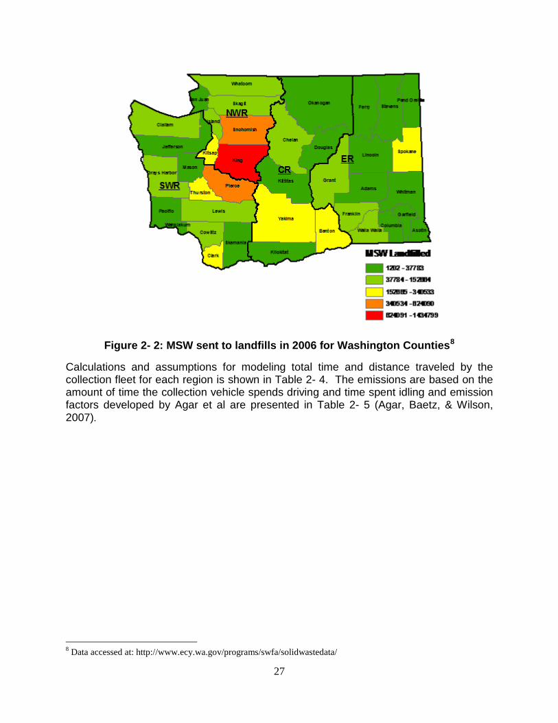
The diversity in collection methods throughout the State makes system level modeling extremely complex. Figure 2- 2 shows the amount of MSW landfilled in 2005 for each county. The majority of the waste generated in Washington is from the western portion of the State, where majority of the population is located in dense urban areas. In order to simplify the model, average regional classifications were developed for the State. The first step was to separate each county into one of three regional classifications based on waste generation. The counties having an annual MSW generation rate of 100,000 MT or more, 10,000 to 100,000 MT, and less than 10,000 MT, were classified as a high, medium, or low generation area, respectively. Annual MSW, MWP, and yard waste generated for each county were calculated based on annual data for MSW sent to landfills7

7 Data accessed at: http://www.ecy.wa.gov/programs/swfa/solidwastedata/

and biomass inventory data for the State (Frear, Zhao, Fu, Richardson, & Fuchs, 2005). Assuming weekly collection, the average amount of waste collected per single-family household per week is calculated. A linear probability model developed by Wilson and Baetz (Wilson & Baetz, 2001), is used to determine the total fleet route size when it is limited by collection volume constraints. The model calculates the size of the route, the number of vehicles required per fleet, the total time and distance traveled by the entire fleet, and the emissions for the entire fleet per metric ton of waste collected.

27

Figure 2- 2: MSW sent to landfills in 2006 for Washington Counties8

Calculations and assumptions for modeling total time and distance traveled by the collection fleet for each region is shown in

Table 2- 4. The emissions are based on the amount of time the collection vehicle spends driving and time spent idling and emission factors developed by Agar et al are presented in Table 2- 5 (Agar, Baetz, & Wilson, 2007).

8 Data accessed at: http://www.ecy.wa.gov/programs/swfa/solidwastedata/

28

Table 2- 4: Collection LCI inputs (Environmental flows are all based on 1 MT of waste hauled)

MSW Recycle YW MSW Recycle YW MSW Recycle YW

Calculations Unit High High High Medium Medium Medium Low Low Low

Avg. Waste Collected annually MT/year 400,000 90,000 120,000 45,000 10,000 15,000 3,000 750 1,000

Avg. Housing households 200,000 200,000 200,000 25,000 25,000 25,000 4,000 4,000 4,000

Vehicle Capacity, (k) m3 32.7 19.6 6.54 32.7 19.6 6.54 32.7 19.6 6.54

Compaction ratio, (p) 3 3 3 3 3 3 3 3 3

Set out rate, (ϕ) 0.9 0.4 0.3 0.9 0.4 0.2 0.9 0.4 0.1

Stops made, (Xf) stops/route 757 2,270 582 454 1,816 454 908 3,632 908

No. of residences past, (Nf) house/route 841 5,674 1,940 504 4,539 2,270 1,009 9,079 9,079

Distance btwn houses, (S) m 5 5 5 15 15 15 30 30 30

Maximum Velocity, (V) m/s 4 4 4 4 4 4 4 4 4

Acceleration, (a) m/s2 1 1 1 1 1 1 1 1 1

Stop spacing Condition 4 4 4 2 2 2 1 1 1

Mean stop-to-stop travel time sec 5 7 7 8 9 8 12 23 79

Avg. Loading time per stop, lt sec. 20 20 20 20 20 20 20 20 20

Total Route time hrs/route 5.2 16.7 4.4 3.5 14.4 3.6 8.2 43.1 25.0

Vehicles required per route Veh./route 1 3 1 1 3 1 2 8 5

Number of routes per week Routes/week 297 44 129 59 7 13 6 1 1

Total Route time for fleet hrs/week 1,541 2,212 572 211 286 47 97 228 83

Total Distance traveled for fleet km/week 22,190 31,849 8,235 3,033 4,125 680 1,397 3,283 1,188

Diesel Fuel Consumption BTU 54,043 387,842 77,142 36,935 334,913 41,427 170,096 2,665,425 723,347

CO2 g 4,065 29,175 5,803 2,778 25,193 3,116 12,795 200,502 54,413

CH4 g 0.19 1.39 0.28 0.13 1.20 0.15 0.61 9.55 2.59

N20 g 0.12 0.85 0.17 0.08 0.74 0.09 0.37 5.88 1.59

NMVOC g 0 0 0 0 0 0 0 0 0

CO g 202 1,451 289 138 1,253 155 637 9,975 2,707

NOX g 230 1,650 328 157 1,424 176 723 11,336 3,076

PM10 g 4.2 30.3 6.0 2.9 26.1 3.2 13.3 208.1 56.5

PM2.5 g 0 0 0 0 0 0 0 0 0

SOx g 0 0 0 0 0 0 0 0 0

Environmental Flows

29

Table 2- 5: Commercial waste vehicle collection emission factors.

Self-haul Self-haul is based on the assumption that passenger or light-duty vehicles are used to transport waste to an intermediate processing facility. It is assumed that the maximum waste that can be hauled per trip is roughly 400 lbs [king county]. The average distance a self-haul vehicle travels is assumed to vary by the regional population density. The distance generators are willing to travel, for high, medium, and low generation regions, is assumed to be 5, 7.5, and 10 miles, respectively. The average fuel efficiency is 24.8 miles per gallon based on the GREET model (USDOE, 2006). Emissions for passenger vehicles are based upon a GM study released in 2005 (Brinkman, Wang, Weber, & Darlington, 2005). Table 2- 6 summarizes the major LCI inputs for self-haul.

Table 2- 6: Summary of LCI inputs for Self-haul

Activity Unit Idling Driving

Percent of time spent per activity 52% 48%

Proportion of fuel consumed 16% 84%

Avg. Rate of Fuel Consumption L/hr & km/L 3.1 0.9

CO2 g/L 2,730 2,730

CH4 g/L 0.13 0.13

N20 g/L 0.08 0.08

CO g/L & g/km 94.6 26.6

NOX g/L & g/km 144 6.68

PM10 g/L & g/km 2.57 0.17

Emission Factors

Units High Medium Low

Vehicle Type Passenger Passenger Passenger

Maximum Waste hauled per trip kg/trip 175.5 175.5 175.5

Distance traveled to facil ity km/MT 45.8 68.7 91.7

Average Fuel efficiency mpg 24.8 24.8 24.8

Fuel TypeConventional

RFGConventional

RFGConventional

RFG

RFG Fuel Lower Heating Value BTU/gal 115,500 115,500 115,500

Environmental Flows

CO2 kg/km 19.56 19.56 19.56

CH4 kg/km 0.108 0.108 0.108

N2O kg/km 0.00033 0.00033 0.00033

NMVOC kg/km 0.0235 0.0235 0.0235

CO kg/km 0.0117 0.0117 0.0117

NOx kg/km 0.0441 0.0441 0.0441

PM10 kg/km 0.00934 0.00934 0.00934

PM2.5 kg/km 0 0 0

SOx kg/km 0.0270 0.0270 0.0270

30

Intermediate Waste Processing Intermediate waste processing includes the handling of waste received at transfer stations, material recovery facilities (MRF), and intermodal rail-yard. An LCI model was created for these three facilities operations, including energy, fuel consumption and emissions from equipment. The module does not include facility construction or building operations, such as, lighting or heating/cooling loads.

Transfer Stations Three designs were used for the transfer station, depending on the regional classification, as with the collection model. For larger areas, additional processing equipment is required for handling approximately 350 metric tons of waste per hour. For our model we assume that transfer stations are only used for MSW and yard waste. The general design for transfer stations is based on EPA recommendations (USEPA, 2002). The design for large transfer stations includes a tipping floor, where vehicles dump incoming waste, front-end loaders, to move waste from the tipping floor into compactors, and finally compacted waste is transferred to long-haul vehicles were it is sent to a final processing facility. The flow diagram for a large transfer station is shown in Figure 2- 3. Medium and small transfer stations are assumed to be designed so that waste collection vehicles can off-load incoming waste directly into compactors, so no front-end loader is required. The LCI module for transfer stations includes the equipment operations on-site and the production of fuel and energy. Operational emissions for diesel equipment were based on calculations from EPA emission factors for non-road CI spark ignition engines and the equations below (USEPA, Exhaust and crankcase emission factors for nonroad engine modeling - compression ignition, 2004). Fuel and electricity pre-combustion emissions are from GREET 1.7.

Figure 2- 3: Process flow diagram for large capacity transfer station.

The equation used to calculate fuel consumption in BTU per metric ton is,

31

where: EF = the emission factor in (lb/hp-hr) 453.6 = the conversion from lb to grams LHV = lower heating value of fuel (BTU/gal) ρ = the density of fuel (grams/gal) HP = horsepower of the engine CF = capacity factor for equipment (MT/hr)

Similar, for the calculation for tailpipe emissions in grams per metric ton is,

where: EF = the emission factor in (g/hp-hr) HP = horsepower of the engine CF = capacity factor for equipment (MT/hr)

Sulfur dioxide emissions are used for SOx emissions.

Table 2- 7: LCI inputs for transfer station equipment.

Intermodal rail-yard A significant amount of waste is exported from Washington into neighboring States. This waste is commonly transported long distances by train. In order to transfer waste on and off a train, a staging area is required. The intermodal rail-yard serves as a staging point connecting the transfer station to the train. The LCI module is based off of the Seattle Rail-yard system, as described in an online article (Harder, 1994). The rail-yard LCI includes trucks dumping waste from transfer station to loading area, lift trucks than move waste containers on and off the train. At the landfill site yard-goats transport the containers from the receiving area to the landfill loading area. Two tippers are used to dump the waste onto the landfill site. Emissions include equipment use, fuel and

unitFront-End

LoaderCompactor

(Small)Compactor (Medium)

Compactor (Large)

Number of Units 7 4 2 1

Capacity MT/hr 50 10 50 100

Engine/Motor Size HP 250 82 140 213

Fuel Type Diesel Electricity Electricity Electricity

Environmental Flows

Total Energy BTU 36,106 23,188 15,836 24,093

CO2 g 2,653

CO g 0.40

NOx g 12.5

PM10 g 0.36

PM2.5 g 0.35

SOx g 0.003

32

energy production, and transportation emissions. Equipment inventory data is shown in Table 2- 8, while the process is shown in Figure 2- 4.

Table 2- 8: LCI input data for intermodal rail-yard equipment.

Figure 2- 4: Process flow diagram for intermodal rail-yard.

Material Recovery Facility The model for a MRF was developed based upon the work of Tchobanoglous et al (Tchobanoglous, Theisen, & Vigil, 1993). The model includes typical unit processes of

unit Yard Goat Lift Truck Tippers

Number of Units 2 2 2

Capacity MT/hr 257 257 257

Engine/Motor Size HP 220 250 210

Fuel Type Diesel Diesel Diesel

Environmental Flows

Fuel Consumption BTU 6,182 7,025 5,901

CO2 g 454 516 434

CO g 0.068 0.077 0.065

NOx g 2.15 2.44 2.05

PM10 g 0.062 0.071 0.059

PM2.5 g 0.060 0.069 0.058

SOx g 0.00045 0.00052 0.00043

33

a MRF for the separation of recycled paper, plastic, glass, and metals. Figure 2- 5 shows a process diagram for the MRF, with processes shaded in gray specific to mixed waste paper operations. Recyclables are received in the tipping area, where front-end loaders move material onto the first picking conveyer. Bags are assumed to be opened automatically by a bag opener (modeled as a trommel screen). Large items and old corrugated cardboard (OCC) are first removed manually from the stream. The remaining waste passes through a trommel screen, where it is assumed that paper, plastics and metals, and glass are separated. The paper then goes through another round of manual picking to separate the paper by grade (Paperboard, High grade, newsprint, and mixed waste). The picking rate is 2.5 tons per person per hour and is assumed to have 80 percent recovery efficiency. Each product is then baled and sold off to final processors. Data from a King County2005 survey of MRFs (Cascadia Consulting Group, inc., 2006) was used to estimate the characteristics of recovered mixed waste paper. The survey estimated that 29 percent of the mass coming out of an MRF is attributed to mixed waste paper product. LCI data for the MRF was allocated for MWP based on the product output.

Figure 2- 5: Process flow diagram for Material Recovery Facility (MRF).

34

Table 2- 9: LCI input for select MRF equipment and operations for MWP

processing.

Landfill This section describes the module for waste sent to a landfill. The unit processes include: landfill daily operations, landfill gas generation/collection, leachate generation, and waste water treatment.

Daily Operations at Landfill The daily operations of the landfill consist of receiving waste from long-haul vehicles, placement of waste in landfill cell, and applying a daily cover to the compacted waste. The model assumes a landfill capacity of 1800 metric tons of MSW per day. In comparison, the three largest landfills, Cedar Hills, Columbia Ridge, and Roosevelt, receive an estimated 2800, 2300, and 3300 tons of waste per day, respectively9

Table 2- 10

. This corresponds to approximately 400 square meters per day or a tenth of an acre per day. The waste is received at the cell location, spread out, compacted, and covered in soil and a High Density Polyethylene (HDPE) liner. It was determined that each cell requires 328 grams of HDPE per metric ton of waste. Equipment operations include: scraper, compactor, motor grader, track loader, track tractor, articulated truck, rubber tire loader, and a water truck. The emissions from vehicle operations were based on EPA Tier-4 emissions data for crank-shaft engines used in the EPA NONROAD (data presented in Appendix C) and equations presented earlier. gives the LCI inputs and emissions associated with landfill equipment. LCI data for HDPE and non-road diesel consumption is from GREET 1.7.

9 Data accessed at: http://www.ecy.wa.gov/programs/swfa/solidwastedata/

unitFront-End

Loader ForkliftBag

BreakerConveyor

Belt Picking BeltTrommel

Screen Baler

Number of Units 4 2 1 1 2 1 1

Capacity MT/hr 36.302121 108.7785 36.302121 36.302121 36.302121 37.4 108.7785

Engine/Motor Size HP 95 50 0.03 0.03 0.03 30 55

Fuel Type Diesel Diesel Electricity Electricity Electricity Electricity Electricity

Environmental Flows

Fuel Consumption BTU 21,009 3,690 2.34 2.34 2.34 2,268 1,429

CO2 g 1,544 271

CO g 0.66 0.75

NOx g 7.88 2.18

PM10 g 0.22 0.091

PM2.5 g 0.21 0.089

SOx g 0.00154 0.00027

35

Table 2- 10: LCI inputs for Landfill equipment (all fuel consumption and emissions per

unit).

Landfill Gas Collection and Electricity Production According to the U.S. EPA all landfills constructed in after 1991 with total capacities greater than 2.5 million cubic meters are required to install landfill gas collection systems (USEPA, 1999). Therefore, landfill gas generation and collection was included, and modeled based on work developed for the MSW-DST model [ (Sich & Barlaz, 2000), (Thorneloe, Weitz, & Jambeck, 2007)]. The general equation for landfill gas generation per metric ton of waste placed is given as,

Where: k = first order decay rate, t2 = time when model stops, t1 = time when model begins, s = first order phase constant, Lo = the landfill gas potential.

A first order decay rate of 0.04/yr was assumed based on EPA AP-42 recommendation for areas with rainfall greater than 25 inches per year (USEPA, 1995). The first order phase constant of 1, with landfill gas collection occurring in three periods is assumed. Period 1 is the first five years from the initial placement of waste, the second from 5 – 40 years, and the third collection from 40 – 80 years. The overall modeling period for landfill gas generation is 100 years. The landfill gas potential is calculated based on decomposition factors published (Barlaz, 2006) and an MSW composition from a King County characterization study (Cascadia Consulting Group, Inc., 2004). Material decomposition factors and MSW composition for degradable components are shown in Table 2- 11. Total landfill gas potential is estimated as 83.1 cubic meters per metric ton.

unit Scraper CompactorMotor grader

Track Loader

Track Tractor

Articulated Truck

Rubber Tire

LoaderWater Truck

Number of Units 1 1 1 1 1 1 1 1

Capacity MT/hr 200 200 200 200 200 200 200 200

Engine/Motor Size HP 462 354 297 239 310 317 180 180

Fuel Type Diesel Diesel Diesel Diesel Diesel Diesel Diesel Diesel

Fuel Consumption: BTU 16,681 12,782 10,724 8,629 11,193 11,446 6,499 6,499

CO2 g 1,226 939 788 634 822 841 478 478

CO g 0.206 0.158 0.118 0.095 0.138 0.141 0.072 0.072

NOx g 5.79 4.44 3.72 3.00 3.89 3.98 2.26 2.26

PM10 g 0.168 0.129 0.108 0.087 0.113 0.115 0.066 0.066

PM2.5 g 0.163 0.163 0.105 0.084 0.109 0.112 0.064 0.064

SOx g 0.00122 0.00122 0.00079 0.00063 0.00082 0.00084 0.00048 0.00048

Environmental Flows

36

EPA estimates average landfill gas potential is approximately 100 cubic meters per metric ton (USEPA, 1999). Furthermore it was assumed that landfill gas is 55% methane, and 45% carbon dioxide.

Table 2- 11: Decomposition factors, MSW composition, and decomposition emissions for Washington MSW components.

Based on an estimated efficiency of landfill gas collection (assumed 75% for all periods), the total landfill gas collected is calculated. It is assumed that during the first and last period the gas was collected and flared, while in the second period the gas is combusted for electricity production. This is in line with work presented by Obersteiner et al, that assumes the second period of landfill gas generation is the most useful for electricity production (Obersteiner, Binner, Mostbauer, & Salhofer, 2007). Total emissions from the landfill for all three periods including losses from inefficiencies were calculated and electricity generation was estimated based on an assumed ICE efficiency of 33%. Total electricity production from landfill gas is estimated as 251,800 BTU per metric ton of MSW. The amount of landfill gas generated and collected is shown below in Figure 2- 6.

Figure 2- 6: Model for landfill gas generation and collection.

Decomp. Factor

MSW Composition WA-MSW

g-CH4/Kg % g-CH4/Kg

Grass 96 2.5% 2.4

Leaves 45 2.5% 1.1

Branches 40 1.8% 0.7

Food Waste 197 20.0% 39.4

Coated Paper 56 14.1% 7.9

Newsprint 50 2.7% 1.4

OCC 100 4.6% 4.6

Office Paper 142 1.6% 2.3

MSW Components

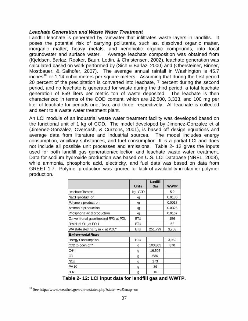
37

Leachate Generation and Waste Water Treatment Landfill leachate is generated by rainwater that infiltrates waste layers in landfills. It poses the potential risk of carrying pollutants, such as, dissolved organic matter, inorganic matter, heavy metals, and xenobiotic organic compounds, into local groundwater and surface water. Average leachate composition was obtained from (Kjeldsen, Barlaz, Rooker, Baun, Ledin, & Christensen, 2002), leachate generation was calculated based on work performed by (Sich & Barlaz, 2000) and (Obersteiner, Binner, Mostbauer, & Salhofer, 2007). The average annual rainfall in Washington is 45.7 inches10

An LCI module of an industrial waste water treatment facility was developed based on the functional unit of 1 kg of COD. The model developed by Jimenez-Gonzalez et al (Jimenez-Gonzalez, Overcash, & Curzons, 2001), is based off design equations and average data from literature and industrial sources. The model includes energy consumption, ancillary substances, and fuel consumption. It is a partial LCI and does not include all possible unit processes and emissions.

or 1.14 cubic meters per square meters. Assuming that during the first period 20 percent of the precipitation is converted into leachate, 7 percent during the second period, and no leachate is generated for waste during the third period, a total leachate generation of 859 liters per metric ton of waste deposited. The leachate is then characterized in terms of the COD content, which are 12,500, 3,333, and 100 mg per liter of leachate for periods one, two, and three, respectively. All leachate is collected and sent to a waste water treatment plant.

Table 2- 12 gives the inputs used for both landfill gas generation/collection and leachate waste water treatment. Data for sodium hydroxide production was based on U.S. LCI Database (NREL, 2008), while ammonia, phosphoric acid, electricity, and fuel data was based on data from GREET 1.7. Polymer production was ignored for lack of availability in clarifier polymer production.

Table 2- 12: LCI input data for landfill gas and WWTP.

10 See http://www.weather.gov/view/states.php?state=wa&map=on

UnitsLandfill

Gas WWTP

Leachate Treated kg - COD 5.2

NaOH production kg 0.0136

Polymers production kg 0.0013

Ammonia production kg 0.0326

Phosphoric acid production kg 0.0167

Conventional gasoline and RFG, at POU BTU 156

Residual Oil, at POU BTU 52

WA state electricity mix, at POU* BTU 251,799 3,753

Energy Consumption BTU 3,962

CO2 (biogenic)** g 103,805 870

CH4 g 16,505

CO g 536

NOx g 173

PM10 g 36

SOx g 10

Environmental Flows

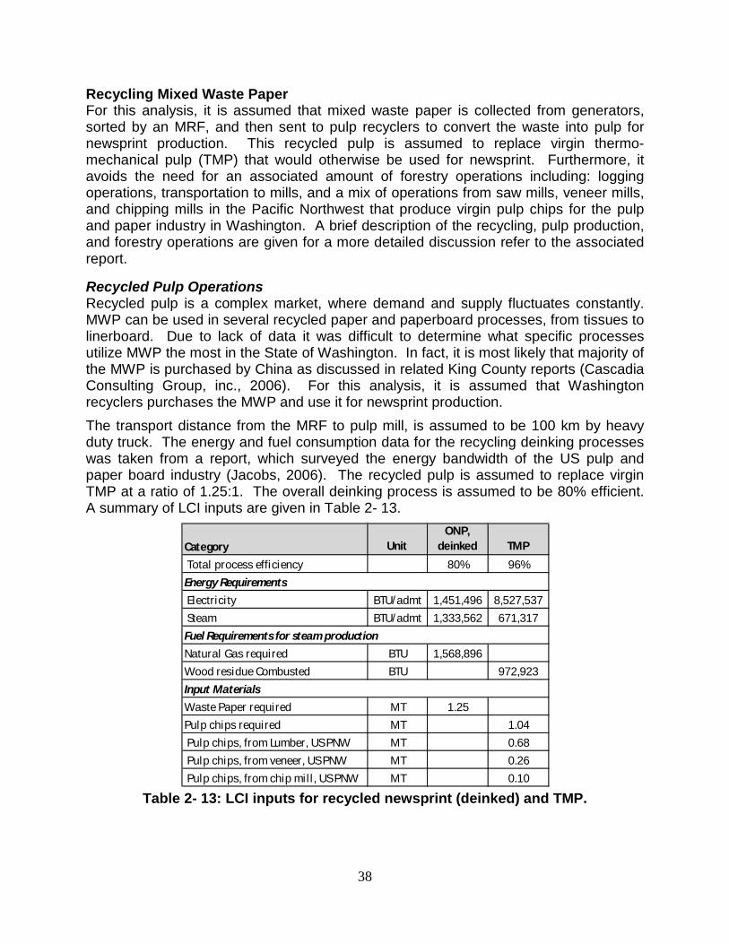
38

Recycling Mixed Waste Paper For this analysis, it is assumed that mixed waste paper is collected from generators, sorted by an MRF, and then sent to pulp recyclers to convert the waste into pulp for newsprint production. This recycled pulp is assumed to replace virgin thermo-mechanical pulp (TMP) that would otherwise be used for newsprint. Furthermore, it avoids the need for an associated amount of forestry operations including: logging operations, transportation to mills, and a mix of operations from saw mills, veneer mills, and chipping mills in the Pacific Northwest that produce virgin pulp chips for the pulp and paper industry in Washington. A brief description of the recycling, pulp production, and forestry operations are given for a more detailed discussion refer to the associated report.

Recycled Pulp Operations Recycled pulp is a complex market, where demand and supply fluctuates constantly. MWP can be used in several recycled paper and paperboard processes, from tissues to linerboard. Due to lack of data it was difficult to determine what specific processes utilize MWP the most in the State of Washington. In fact, it is most likely that majority of the MWP is purchased by China as discussed in related King County reports (Cascadia Consulting Group, inc., 2006). For this analysis, it is assumed that Washington recyclers purchases the MWP and use it for newsprint production. The transport distance from the MRF to pulp mill, is assumed to be 100 km by heavy duty truck. The energy and fuel consumption data for the recycling deinking processes was taken from a report, which surveyed the energy bandwidth of the US pulp and paper board industry (Jacobs, 2006). The recycled pulp is assumed to replace virgin TMP at a ratio of 1.25:1. The overall deinking process is assumed to be 80% efficient. A summary of LCI inputs are given in Table 2- 13.

Table 2- 13: LCI inputs for recycled newsprint (deinked) and TMP.

Category UnitONP,

deinked TMP

Total process efficiency 80% 96%

Electricity BTU/admt 1,451,496 8,527,537

Steam BTU/admt 1,333,562 671,317

Natural Gas required BTU 1,568,896

Wood residue Combusted BTU 972,923

Waste Paper required MT 1.25

Pulp chips required MT 1.04

Pulp chips, from Lumber, US PNW MT 0.68

Pulp chips, from veneer, US PNW MT 0.26

Pulp chips, from chip mill , US PNW MT 0.10

Fuel Requirements for steam production

Energy Requirements

Input Materials

39

Virgin Pulp Production Virgin paper production begins with forestry operations. In the United States, majority of the virgin pulp fibers come from the Pacific Northwest or the Southeastern region of the country. In the Pacific Northwest, majority of the wood is used for forestry products, such as, lumber, plywood, chips, etc. Pulp mills purchase pulp chips from saw and chip mills. The LCI data presented includes forestry operations, sawmill, chip mills, and pulp mills.

Thermo-mechanical Pulping TMP is the most common mechanical pulping process used to produce virgin newsprint. It produces the highest grade of pulp from mechanical pulping without additional bleaching. The TMP process uses steam to soften wood chips before using a mechanical pulper. The process is the most energy intensive of the mechanical pulps, requiring intensive electricity consumption. LCI data for thermo-mechanical pulping comes from the industrial survey (Jacobs, 2006).

Forestry Operations Forestry LCI data was from US LCI database for average intensity softwood logging in the Pacific Northwest. US LCI database inventory data was also used for saw mill operations for lumber production, veneer production, and chipping and debarking.

Composting Commercial compost facilities in Washington, such as Cedar Groves, process collected yard waste. In our assessment we assume that a compost facility creates commercial compost from yard waste that competes with commercial fertilizer production as a soil amendment.

Windrow Turning Facility Composting is the biological decomposition of organic matter into nutrients, which can be used as a soil nutrient or amendment. An LCI model for a yard waste compost

UnitsLumber

OperationsPlywood

OperationsChipping

Operatons

Product Outputs

Pulp chips, from rough green Lumber, US PNW kg 384

Pulp chips, at plywood plant, US PNW kg 0.34

Pulp chips, from Chipping Mill , US PNW kg 1

Inputs

Softwood logs m3 0.81 0.0025 0.0025

Conditioned log, at plywood plant, US PNW kg 6

WA state electricity mix, at POU BTU 79,101 933 176

US non-road diesel, at POU BTU 16,657 206 62.6

LPG, at POU BTU 3.07 85.5

Gasoline (combusted in equipment) BTU 1,564

Air Emissions

PM10 (Dust) g 0.56 0.044

VOC g 1.55

40

facility was developed for the US EPA (Komilis & Ham, 2000), and adapted for our purposes. The model includes equipment operations for a commercial windrow facility and decomposition emissions from converting yard waste into commercial compost. The facility modeled in this study is assumed to operate at a capacity of 130,000 MT per year. Yard waste is transported from a transfer station to the compost facility. It is assumed that on average a compost facility will accept materials within 50 kilometers from its facility in order for it to operate cost efficiently. The yard waste is moved from the tipping floor into a tub grinder where oversized material is shredded. It is then placed in windrow piles where it has a residence time of 16 weeks. No water or nutrients are added to the compost piles, since the yard waste is assumed to have a moisture content of 60 percent. The piles are turned monthly with a front-end loader. Finally the compost is passed through a trommel screen to capture the fine fraction product compost. It is estimated that 46 percent of incoming yard waste is converted into compost, while 4 percent is sent to landfill as waste. Emissions from the biological decomposition of waste material into product compost, and equipment energy consumption and emissions were included in the assessment.

Figure 2- 7: Process flow diagram for windrow compost facility

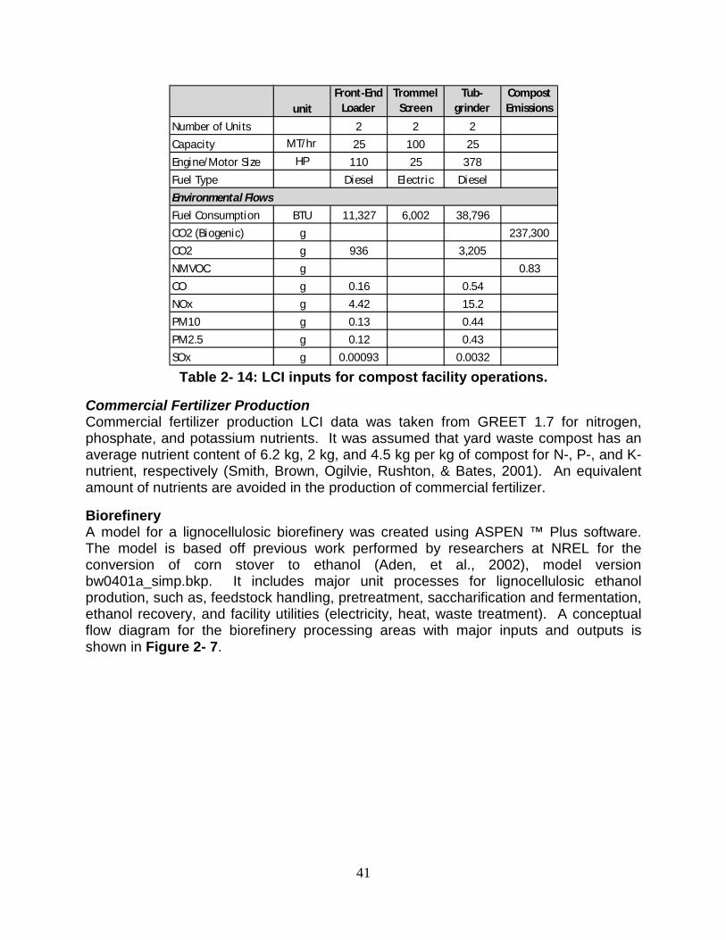
41

Table 2- 14: LCI inputs for compost facility operations.

Commercial Fertilizer Production Commercial fertilizer production LCI data was taken from GREET 1.7 for nitrogen, phosphate, and potassium nutrients. It was assumed that yard waste compost has an average nutrient content of 6.2 kg, 2 kg, and 4.5 kg per kg of compost for N-, P-, and K-nutrient, respectively (Smith, Brown, Ogilvie, Rushton, & Bates, 2001). An equivalent amount of nutrients are avoided in the production of commercial fertilizer.

Biorefinery A model for a lignocellulosic biorefinery was created using ASPEN ™ Plus software. The model is based off previous work performed by researchers at NREL for the conversion of corn stover to ethanol (Aden, et al., 2002), model version bw0401a_simp.bkp. It includes major unit processes for lignocellulosic ethanol prodution, such as, feedstock handling, pretreatment, saccharification and fermentation, ethanol recovery, and facility utilities (electricity, heat, waste treatment). A conceptual flow diagram for the biorefinery processing areas with major inputs and outputs is shown in Figure 2- 7.

unitFront-End

LoaderTrommel

ScreenTub-

grinderCompost Emissions

Number of Units 2 2 2

Capacity MT/hr 25 100 25

Engine/Motor Size HP 110 25 378

Fuel Type Diesel Electric Diesel

Fuel Consumption BTU 11,327 6,002 38,796

CO2 (Biogenic) g 237,300

CO2 g 936 3,205

NMVOC g 0.83

CO g 0.16 0.54

NOx g 4.42 15.2

PM10 g 0.13 0.44

PM2.5 g 0.12 0.43

SOx g 0.00093 0.0032

Environmental Flows

42

Figure 2- 8: Major process flow diagram for biorefinery model.

Lignocellulosic composition for the three feedstock materials is shown in Table 2- 15. The composition for MSW, and MWP were determined experimentally by researchers at the University of Washington College of Forest Resources, while the composition for yard waste is based off of literature values. The theoretical yields for MSW, MWP, and YW are calculated as 151, 118, and 70 gals per ton, respectively. It is assumed that the farthest distance feedstock can be transported and still remain economical is 50 miles this is assumed to be the same here. The capacity for lignocellulosic ethanol production is 98,040 kg/hr, however, the capacity for the feedstock handling area is actually larger to include removal of contaminants from the feed stream.

Table 2- 15: Lignocellulosic composition and theoretical yield for ethanol feedstocks.

Lignocellulosic Components MSW Waste Paper

Cellulose 74.0% 64.3% 44.7% Xylan 7.3% 7.8% 14.6% Arabinan 0.8% 0.9% 0.8% Mannan 7.9% 4.4% 2.2% Galactan 0.5% 0.3% 1.0% Lignin 7.7% 21.1% 26.4% Ash 1.8% 1.1% 1.7% Moisture 0.0% 5.0% 0.0% Other 0.0% 0.0% 8.6% Theoretical Yield (gal/ton) 156.7 134.6 110

43

Feedstock Handling & Pretreatment Each solid waste stream requires different feedstock handling to remove various contaminants (metals, plastics, oversized waste) before it can continue through the ethanol conversion process.

MSW MSW from transfer stations is transported to the biorefinery by heavy-duty trucks. Lignocellulosic portions of incoming MSW material makes up approximately 53 percent of total waste (Cascadia Consulting Group, Inc., 2004). To achieve 98,040 kg/hr of lignocellulosic feedstock approximately 184,286 kg/hr of MSW must be received. This is equivalent to approximately 2,200 MT per day of MSW. Trucks unload waste onto the tipping floor where front-end loaders then transfer the feedstock from the tipping floor to feed conveyors. The waste is conveyed through a bag breaker (modeled as a trommel screen), which tears open plastic bags containing waste and separates the oversized waste from the feedstock. Unprocessed waste is sent to solid waste processing (B100), where it is baled and sent to a landfill. Usable feedstock is dumped onto a drag conveyor belt and passed through a ferrous magnet and eddy current separator to remove ferrous and nonferrous metals. It then passes through a second trommel screen to remove plastics and glass contaminants. The remaining feedstock is sent through the wash table to remove excess dirt and grit. Finally it is passed into two shredders to reduce waste to under 1.5 inches. Shredded feedstock is then sent to pretreatment.

Figure 2- 9: Process diagram for MSW feedstock handling.

44

Paper Paper processing is similar to MSW processing. Baled mixed waste paper is delivered in heavy duty trucks transporting mixed waste paper from an MRF to the biorefinery. Forklifts unload bales from the trucks and transfer to the storage area. Another set of forklifts move the baled mixed paper waste from storage area to the bale unwrapper (modeled as conveyor belt). The loose paper is passed onto a second conveyor which travels through a ferrous magnet. The remaining material is passed into a shredder to reduce size of feedstock. The shredded material is sent to the hydrapulper for pretreatment. Waste water from pretreatment is sent to A600 waste water treatment, while solid wastes are processed in a separate area.

Figure 2- 10: Process flow diagram for MWP feedstock handling.

Yard Waste Yard waste is shipped from transfer station to biorefinery in heavy duty truck and dumped onto the tipping floor. A front-end loader is used to move the organics from the tipping floor to feed conveyor. The organics are conveyed through a bag breaker to free up any bagged yard waste. The loose feedstock passes through magnetic separation to remove any metals and then goes through a wash table. The washed feedstock passes through primary and secondary shredders to reduce the size to less than 1.5 inches. The shredded feed is sent to steam explosion pretreatment.

45

ASPEN Model Development Feedstock handling was modeled outside the ASPEN model in an associated spreadsheet; this section describes the inputs for the NREL model bw0401a_simp.bkp11

The models for MSW and MWP are essentially the same, in terms of physical treatments. The reactor for pretreatment was modeled as a hydrapulper, instead of a screw press reactor. Sulfuric acid is added to the hydrapulper at a concentration of 3 percent to induce acid hydrolysis and separation of lignin at a temperature of 60oC. The pretreated slurry is sent to saccharification and fermentation. The adjustment to a low pressure hot water system eliminated the use of a distillation economizer, and this process and associated equipment were removed from the analysis. While for yard waste, a steam explosion pretreatment process was modeled and temperatures in the pretreatment reactor were changed to 215oC and 13 atm. In addition, SO2 at a 3 percent concentration was used instead of H2SO4. The remainder of the physical processing is outlined in the NREL model description and is essentially unchanged (Aden, et al., 2002). Changes in conversion rates and chemical loadings are described in Tables 2-14 and 2-15, while model outputs are given in Table 2- 16.

.

11 Accessed at: http://devafdc.nrel.gov/biogeneral/Aspen_Models/

46

Table 2- 16: ASPEN model inputs.

Table 2- 17: Conversion rates for different stages of processing.

Feedstock Type MSW Waste Paper Yard Waste

Moisture Content 20% 5% 60%

Pretreatment Conditions

TypeAcid Hydrolysis in Hydrapulper

Acid Hydrolysis in Hydrapulper

Steam Explosion

Catalyst H2SO4 H2SO4 SO2

Concentration 4% 4% 3%

Residence Time 6 hrs 6 hrs 5 mins

Temperature (deg C) 60 60 215

Pressure (atm) 1 1 12.1

SSF Conditions

Saccharification Type Enzymatic Enzymatic Enzymatic

Enyzme Organism T. Reesei T. Reesei T. Reesei

Enzyme Loading (FPU/g) 20 20 20

Fermentation Bacteria Z. Mobilis Z. Mobilis Z. Mobilis

Residence Time (days) 1 1.5 1.5

Temperature (deg C)

Hydrolysis 65 65 65

Fermentation 41 41 41

Pressure (atm) 1 1 1

Pretreatment Conversions MSW Waste Paper Yard Waste

Cellulose -> C6 sugars 0% 0% 0%

Cellulose -> glucose 0% 0% 0%

xylan -> xylose 84% 62% 75%

C5solid -> C5sugar 59% 72% 75%

C6solid -> C6sugar 12% 27% 0%

SSF Conversions

Cellulose --> Glucose 89% 86% 75%

Hexose --> EtOH 95% 95% 95%

Pentose --> EtOH 85% 85% 85%

Seed Train

Hexose --> EtOH 90% 90% 90%

Pentose --> EtOH 80% 80% 80%

Final Yields

Model yield (gal/ton) 115.8 98.2 72.4

Theoretical Yield (gal/ton) 156.7 134.6 110

Percent of theoretical 74% 73% 66%

47

Table 2- 18: LCI inputs for lignocellulosic ethanol production

U.S. Corn Ethanol Production It is assumed that for every liter of cellulosic ethanol produced, and equal amount of corn ethanol is displaced. For the analysis dry-mill ethanol LCI data from GREET 1.7 is used to represent ethanol. Since majority of the ethanol produced in the U.S. is from this process.

Chemicals Production The life cycle of cellulosic ethanol production requires the use of several chemical inputs. This includes the production of sulfuric acid, lime production, enzyme production, corn steep liquor production, ammonium phosphate, and ethanol denaturant. All chemical LCI input data are given in the associated report.

Sulfuric Acid Production Sulfuric acid is used during the pretreatment of MSW and MWP to weaken the bond between cellulosic material and the lignin structure. It is also used in the overliming process of the biorefinery to remove lime from the product stream and convert it into gypsum. LCI data for sulfuric acid production was taken from GREET 1.7 based on US average electricity grid.

Lime Production Hydrated lime [Ca(OH)2] is used to neutralize the acidity of the liquid waste coming out of the pretreatment process. Residual lime is separated from the solid stream by mixing with sulfuric acid to form gypsum. The co-product gypsum is ignored from the analysis

units MSW Waste Paper Yard Waste

Ethanol Produced kg/hr 29,987 30,218 9,375

Incoming Feedstock kg/hr 184,286 120,590 98,040

Cellulosic Feedstock kg/hr 98,040 98,040 98,040

Transportation Distance km 80 80 80

Chemicals/Fuel Consumption

Sulfuric Acid kg/hr 8,444 10,090 3,325

Hydrated Lime kg/hr 6,095 7,283 358

Corn Steep Liquor kg/hr 1,216 1,445 564

Enzyme kg/hr 23,113 14,108 6,886

Ammonium Phosphate kg/hr 151 180 70

Denaturant kg/hr 1,237 1,247 387

Solid waste kg/hr 86,246 22,550 0

Electricity Consumption/Production

Electricity Produced kW 11,934 34,323 19,731

Electricity Consumed kW 14,656 16,914 9,905

Net Electricity kW -2,722 17,409 9,827

Emissions

CO2 kg/hr 103,514 74,704 48,017

N2 kg/hr 261,249 113,050 118,351

CH4 kg/hr 0.64 0.42 0.17

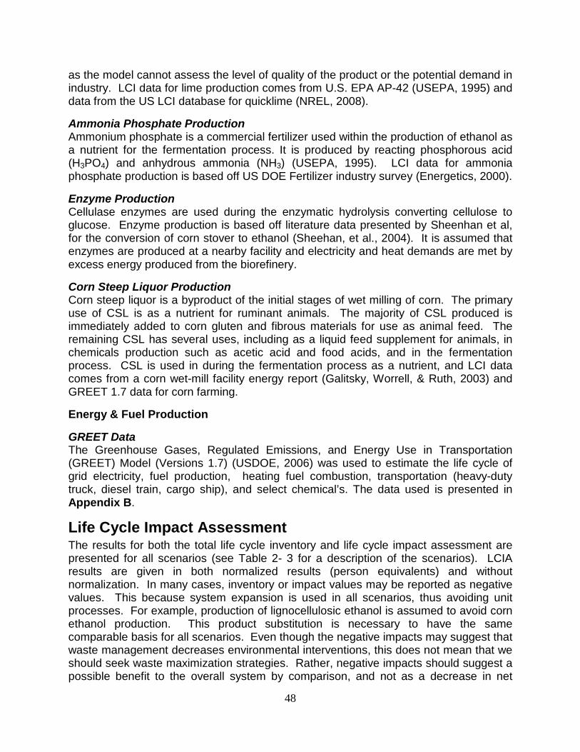
48

as the model cannot assess the level of quality of the product or the potential demand in industry. LCI data for lime production comes from U.S. EPA AP-42 (USEPA, 1995) and data from the US LCI database for quicklime (NREL, 2008).

Ammonia Phosphate Production Ammonium phosphate is a commercial fertilizer used within the production of ethanol as a nutrient for the fermentation process. It is produced by reacting phosphorous acid (H3PO4) and anhydrous ammonia (NH3) (USEPA, 1995). LCI data for ammonia phosphate production is based off US DOE Fertilizer industry survey (Energetics, 2000).

Enzyme Production Cellulase enzymes are used during the enzymatic hydrolysis converting cellulose to glucose. Enzyme production is based off literature data presented by Sheenhan et al, for the conversion of corn stover to ethanol (Sheehan, et al., 2004). It is assumed that enzymes are produced at a nearby facility and electricity and heat demands are met by excess energy produced from the biorefinery.

Corn Steep Liquor Production Corn steep liquor is a byproduct of the initial stages of wet milling of corn. The primary use of CSL is as a nutrient for ruminant animals. The majority of CSL produced is immediately added to corn gluten and fibrous materials for use as animal feed. The remaining CSL has several uses, including as a liquid feed supplement for animals, in chemicals production such as acetic acid and food acids, and in the fermentation process. CSL is used in during the fermentation process as a nutrient, and LCI data comes from a corn wet-mill facility energy report (Galitsky, Worrell, & Ruth, 2003) and GREET 1.7 data for corn farming.

Energy & Fuel Production

GREET Data The Greenhouse Gases, Regulated Emissions, and Energy Use in Transportation (GREET) Model (Versions 1.7) (USDOE, 2006) was used to estimate the life cycle of grid electricity, fuel production, heating fuel combustion, transportation (heavy-duty truck, diesel train, cargo ship), and select chemical’s. The data used is presented in Appendix B.

Life Cycle Impact Assessment The results for both the total life cycle inventory and life cycle impact assessment are presented for all scenarios (see Table 2- 3 for a description of the scenarios). LCIA results are given in both normalized results (person equivalents) and without normalization. In many cases, inventory or impact values may be reported as negative values. This because system expansion is used in all scenarios, thus avoiding unit processes. For example, production of lignocellulosic ethanol is assumed to avoid corn ethanol production. This product substitution is necessary to have the same comparable basis for all scenarios. Even though the negative impacts may suggest that waste management decreases environmental interventions, this does not mean that we should seek waste maximization strategies. Rather, negative impacts should suggest a possible benefit to the overall system by comparison, and not as a decrease in net

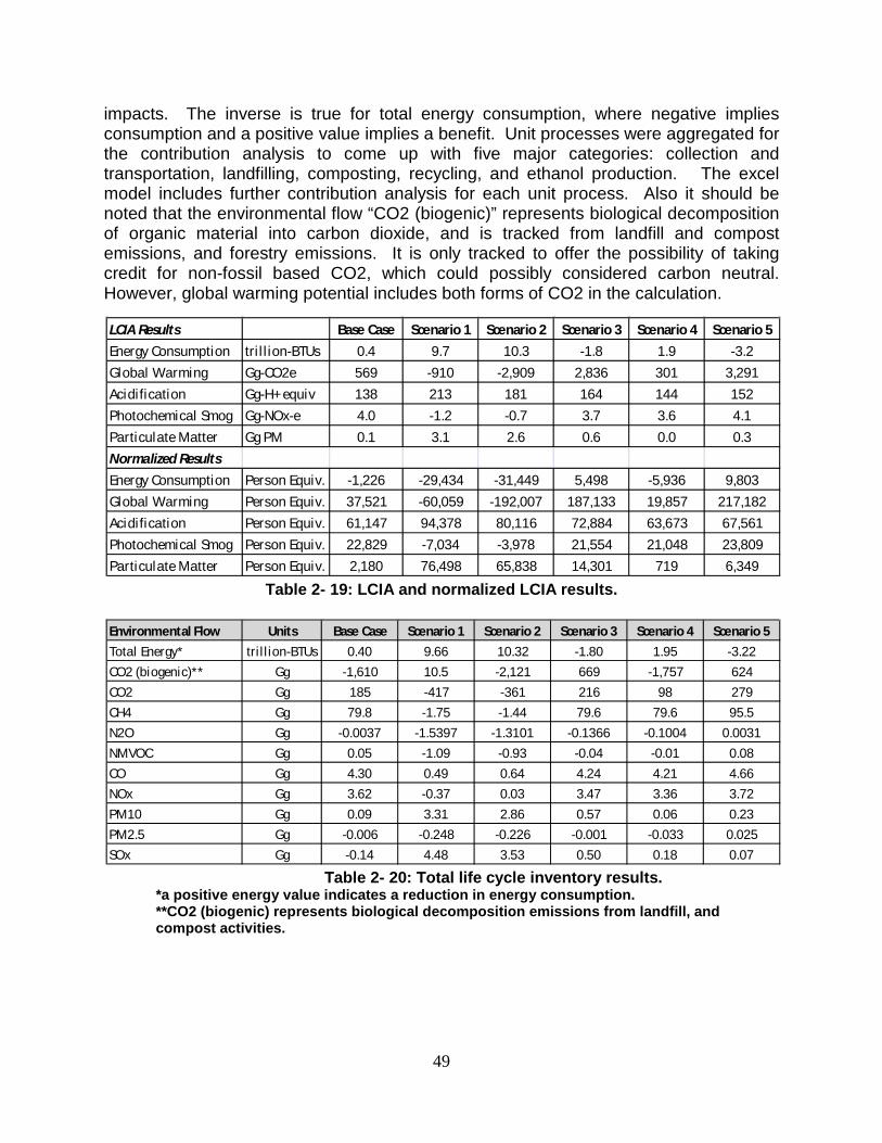
49

impacts. The inverse is true for total energy consumption, where negative implies consumption and a positive value implies a benefit. Unit processes were aggregated for the contribution analysis to come up with five major categories: collection and transportation, landfilling, composting, recycling, and ethanol production. The excel model includes further contribution analysis for each unit process. Also it should be noted that the environmental flow “CO2 (biogenic)” represents biological decomposition of organic material into carbon dioxide, and is tracked from landfill and compost emissions, and forestry emissions. It is only tracked to offer the possibility of taking credit for non-fossil based CO2, which could possibly considered carbon neutral. However, global warming potential includes both forms of CO2 in the calculation.

Table 2- 19: LCIA and normalized LCIA results.

Table 2- 20: Total life cycle inventory results.

*a positive energy value indicates a reduction in energy consumption. **CO2 (biogenic) represents biological decomposition emissions from landfill, and compost activities.

LCIA Results Base Case Scenario 1 Scenario 2 Scenario 3 Scenario 4 Scenario 5

Energy Consumption tril l ion-BTUs 0.4 9.7 10.3 -1.8 1.9 -3.2

Global Warming Gg-CO2e 569 -910 -2,909 2,836 301 3,291

Acidification Gg-H+ equiv 138 213 181 164 144 152

Photochemical Smog Gg-NOx-e 4.0 -1.2 -0.7 3.7 3.6 4.1

Particulate Matter Gg PM 0.1 3.1 2.6 0.6 0.0 0.3

Normalized Results

Energy Consumption Person Equiv. -1,226 -29,434 -31,449 5,498 -5,936 9,803

Global Warming Person Equiv. 37,521 -60,059 -192,007 187,133 19,857 217,182

Acidification Person Equiv. 61,147 94,378 80,116 72,884 63,673 67,561

Photochemical Smog Person Equiv. 22,829 -7,034 -3,978 21,554 21,048 23,809

Particulate Matter Person Equiv. 2,180 76,498 65,838 14,301 719 6,349

Environmental Flow Units Base Case Scenario 1 Scenario 2 Scenario 3 Scenario 4 Scenario 5

Total Energy* tril l ion-BTUs 0.40 9.66 10.32 -1.80 1.95 -3.22

CO2 (biogenic)** Gg -1,610 10.5 -2,121 669 -1,757 624

CO2 Gg 185 -417 -361 216 98 279

CH4 Gg 79.8 -1.75 -1.44 79.6 79.6 95.5

N2O Gg -0.0037 -1.5397 -1.3101 -0.1366 -0.1004 0.0031

NMVOC Gg 0.05 -1.09 -0.93 -0.04 -0.01 0.08

CO Gg 4.30 0.49 0.64 4.24 4.21 4.66

NOx Gg 3.62 -0.37 0.03 3.47 3.36 3.72

PM10 Gg 0.09 3.31 2.86 0.57 0.06 0.23

PM2.5 Gg -0.006 -0.248 -0.226 -0.001 -0.033 0.025

SOx Gg -0.14 4.48 3.53 0.50 0.18 0.07

50

Figure 2- 11: Normalized LCIA results for all impact categories, showing how impacts deviate for each

scenario

Figure 2- 12: Normalized LCIA results, showing how scenarios compare in each impact category.

51

Figure 2- 13: LCIA contribution analysis for Total Energy Consumption

Figure 2- 14: LCIA contribution analysis for Global Warming Potential.

52

Figure 2- 15: LCIA contribution analysis for acidification potential.

Figure 2- 16: LCIA contribution analysis for Photochemical Smog formation.

53

Figure 2- 17: LCIA contribution analysis for total life cycle PM emissions

Figure 2- 18: LCI contribution analysis for total CO2 emissions.

54

Figure 2- 19: LCI contribution analysis for total CH4 emissions.

Figure 2- 20: LCI contribution analysis for total N2O emissions.

55

Figure 2- 21: LCI contribution analysis for total SOx emissions.

Figure 2- 22: LCI contribution analysis for total NOx emissions.

56

Figure 2- 23: LCI contribution analysis for total NMVOC emissions.

Figure 2- 24: LCI contribution analysis for total CO emissions.

57

Process Economics The process modeling that was done for the LCA research was also used to make estimates of the economic viability of converting the three waste streams to ethanol. In this economic analysis we assumed construction of biorefineries that consume about 800,000 tons per year of biomass (either municipal solid waste, paper waste, or yard waste). The cost analysis includes a total project investment based on installed capital cost, variable operating costs, and fixed operating costs for each plant design. From these three factors, a discounted cash flow analysis is performed and the breakeven selling price of ethanol determined.

Methods Total Project Investment The capital cost was determined by estimating the individual equipment costs associated with ethanol production. The cost estimate is classified as class 30 (roughly 30% accuracy) and is to be used for feasibility purposes. Installation factors are used to determine installed costs from purchased equipment costs. The majority of the installation factors were obtained from CHEMSYSTEMS12

Once capital costs were determined for the base year, they were indexed to 2009 using the Chemical Engineering Plant Cost Index. Additional costs are included as fractions of the total capital cost. These costs include warehouse costs, site development, prorateable costs, field expenses, construction, contingency, and a few others. A detailed list of these costs and methods for calculating them can be found in NREL report (Aden, et al., 2002) assessing a biorefinery using cornstover feedstock.

or from equipment vendors.

Variable Operating Costs The variable operating costs are calculated based on the material and energy balance provided by the Aspen models. The costs include raw materials, waste handling charges, and by-product credits as provided by the corn in the ethanol NREL report.

Fixed Operating Costs Fixed operating costs include labor and overhead. Fixed operating costs came from Aden (Aden, et al., 2002) or from Peters (Peters, Timmerhaus, & West, 2003). General overhead is estimated as 60% of the total salaries and covers items such as safety, general engineering, general plant maintenance, payroll overhead (including benefits), plant security, janitorial and similar services, phone, light, heat, and plant communications. Additional maintenance materials were estimated at 2% of total installed cost. Insurance and taxes were estimated at 1.5% of total installed cost.

Discounted Cash Flow Analysis The discounted cash flow analysis is used to find the price of ethanol required for a net present value of $0 after a 20 year plant life and at a discounted cash flow rate of return of 15%. The analysis assumes a federal tax rate of 39%. .

12 http://www.chemsystems.com/

58

Results For each feedstock option, an economic analysis was performed for processes using one of two fermentation organisms; conventional Brewer’s yeast (Saccharomyces cerevisiae) and Zymomonas mobilis. The Brewer’s yeast was assumed to ferment only hexose sugars while Zymomonas was assumed to ferment hexose and pentose sugars according to the yields given by Aden (Aden, et al., 2002). The discounted cash flow analysis for the Brewer’s case resulted in a minimum selling price for ethanol of approximately $1.49 per gallon in the municipal solids waste case. For the case of waste paper and Brewer’s yeast, the minimum selling price is slightly higher at $2.34 per gallon. Lastly, the yard waste feedstock analysis yielded a selling price of $2.92 per gallon. The considerably lower minimum selling price for the municipal solid waste reflects this raw materials ease of conversion and relatively low pentose sugar content. In the Zymomonas case, the minimum selling prices are $1.36, $2.15, and $2.25 for solids waste, waste paper, and yard waste respectively. The lower minimum selling prices for Zymomonas reflect its ability to convert both hexose and pentose sugars. The results for the municipal solids waste process economic analysis in the Brewer’s yeast case are shown in Table 2-21. The feedstock rates for each of the three processes are equal. However, the different yields and compositions will change the economics from case to case. Table 2-21. Summary of Production Rates, Yields, and Converting Costs forMSW Process using Brewer’s Yeast Feedstock Rate (metric ton/day) 2256 Ethanol Production (MM Gal. / Year) 76.8 Ethanol Yield (Gal / Dry US Ton Feedstock) 105.6 Total Equipment Cost (2009 $) $97,000,000 Total Project Investment (2009 $) $168,800,000 Waste Disposal ($/yr) $3,600,000 Fixed Costs ($/yr) $7,600,000 Minimum Ethanol Selling Price ($/gal) $1.49

Similarly, the results for the waste paper process design using Brewer’s yeast are below in Table 2-22.

Table 2-22. Summary of Production Rates, Yields, and Converting Costs for Waste Paper Process using Brewer’s Yeast Feedstock Rate (metric ton/day) 2256 Ethanol Production (MM Gal. / Year) 77.4 Ethanol Yield (Gal / Dry US Ton Feedstock) 89.7 Total Equipment Cost (2009 $) $124,500,000 Total Project Investment (2009 $) $215,200,000 Waste Disposal ($/yr) $4,200,000 Fixed Costs ($/yr) $8,700,000 Minimum Ethanol Selling Price ($/gal) $2.34

59

Lastly, the economic results for the yard waste process design are listed in Table 2-23. The total equipment cost and total project investment for yard waste are somewhat higher due to the addition of a steam gun.

Table 2-23. Summary of Production Rates, Yields, and Converting Costs for Yard waste Process using Brewer’s Yeast Feedstock Rate (metric ton/day) 2256 Ethanol Production (MM Gal. / Year) 20.0 Ethanol Yield (Gal / Dry US Ton Feedstock) 55.0 Total Equipment Cost (2009 $) $123,500,000 Total Project Investment (2009 $) $217,000,000 Waste Disposal ($/yr) $400,000 Fixed Costs ($/yr) $8,000,000 Minimum Ethanol Selling Price ($/gal) $2.92

The three results summary tables for the Zymomonas case are shown in Table 2-24 through Table 2-26 . The yields tend to be slightly higher than in Tables 2-21 – 2-23 due to higher conversions in the fermentation process.

Table 2-24. Summary of Production Rates, Yields, and Converting Costs for MSW Process using Zymomonas Feedstock Rate (metric ton/day) 2256 Ethanol Production (MM Gal. / Year) 84.1 Ethanol Yield (Gal / Dry US Ton Feedstock) 115.8 Total Equipment Cost (2009 $) $93,700,000 Total Project Investment (2009 $) $163,300,000 Waste Disposal ($/yr) $3,600,000 Fixed Costs ($/yr) $7,500,000 Minimum Ethanol Selling Price ($/gal) $1.36

Table 2-25. Summary of Production Rates, Yields, and Converting Costs for Waste Paper Process using Zymomonas Feedstock Rate (metric ton/day) 2256 Ethanol Production (MM Gal. / Year) 84.8 Ethanol Yield (Gal / Dry US Ton Feedstock) 98.2 Total Equipment Cost (2009 $) $121,100,000 Total Project Investment (2009 $) $209,700,000 Waste Disposal ($/yr) $4,200,000 Fixed Costs ($/yr) $8,600,000 Minimum Ethanol Selling Price ($/gal) $2.15

60

Table 2-26. Summary of Production Rates, Yields, and Converting Costs for Yard waste Process using Zymomonas Feedstock Rate (metric ton/day) 2256 Ethanol Production (MM Gal. / Year) 26.3 Ethanol Yield (Gal / Dry US Ton Feedstock) 72.4 Total Equipment Cost (2009 $) $120,600,000 Total Project Investment (2009 $) $212,200,000 Waste Disposal ($/yr) $400,000 Fixed Costs ($/yr) $7,900,000 Minimum Ethanol Selling Price ($/gal) $2.25

Discussion The lowest yield and highest minimum selling price in both the Brewer’s yeast and Zymomonas cases are for the yard waste case. This is largely due to the low 41% conversion of glucose to ethanol in the fermentation step. The high lignin content and relatively low cellulose content make the sugars less accessible for fermentation and therefore the process has lower yields. It is possible that once the process is optimized that these yields may be improved drastically. In contrast, the highest yields and lowest minimum selling price is associated with the solids waste in each case. The sugars in this case are easily accessible and lignin content is low resulting in higher overall yields. Overall, the use of Zymomonas bacteria will result in slightly higher yields and lower prices. This is due to the fermentation of sugars otherwise inaccessible by Brewer’s yeast. It is unclear if Zymomonas would perform as well as the time tested Brewer’s yeast in a commercial operation. Overall the economic analysis suggests that conversion of municipal waste is economically viable. Further economic analysis would be required, however, for a more definitive conclusion. For example, more accurate capital cost estimates can be made especially in the case of the steam gun in the yard waste case. Also, the cost of raw materials could be more accurately estimated by factoring in transportation costs. It is recommended that these details be well established to improve the accuracy of the economic results.

Recommendations & Conclusion The LCA modeled is presented as a “what-if” scenario. It looks retrospectively at Washington’s waste management strategies and analyses what would happen if the waste was treated by sending it to a lignocellulosic biorefinery. Each waste management strategy, including landfill, has the potential to create a product that could avoid the production of another similar product. Compost can replace fertilizer, recycle waste paper can replace virgin pulp and forestry operations, landfilled waste can generate landfill gas, which can be combusted for electricity production. The question is whether, avoiding corn ethanol production with lignocellulosic ethanol has a greater benefit than the others. From our analysis we can make several conclusions and recommendations:

61

1. Municipal solid waste seems to offer the greatest potential as both a waste management strategy and for bio-fuel production. With over 4 million metric tons of MSW generated in 2007, there is enough lignocellulosic material available to meet the demands of a large capacity biorefinery within the State.

2. The greatest contributor to ethanol production environmental flows is chemicals production, specifically lime production. On the other hand, avoidance of dry-mill corn ethanol greatly reduces the environmental flows for ethanol production.

3. Landfilled waste offers the least benefit overall, even with production of electricity and avoidance of Washington electric grid. This is related to the fact that the Washington electric grid is largely dominated by clean hydropower and offers little benefit from avoidance.

Based on these conclusions and the findings from the LCA it is recommended that bio-fuel production from lignocellulosic rich MSW should be pursued over the other waste streams. Mixed waste paper, although has benefits for ethanol production, seems to have greater benefits for replacing virgin pulp. Likewise yard waste seems to offer greatest benefits as a compost than as solely as an ethanol fuel source. It is also possible that some combination of the waste streams be used.

The LCA is incomplete as it does not include all possible environmental flows and is only restricted to nine air emissions and total energy. Furthermore, it does not include all possible technology for ethanol production, composting, and especially for recycling.

The process economic analysis suggests that the conversion of MSW to ethanol is economically viable. The ease of conversion and good process yields for this raw material results in reasonable minimum ethanol selling prices even when using conventional Brewer’s yeast as a fermentation organism.

62

References Aden, A., Ruth, M., Ibsen, K., Jechura, J., Neeves, K., Sheehan, J., et al. (2002). Lingocellulosic biomass to ethanol process design and economics utilizing co-current dilute acid prehydrolysis and enzymatic hydrolysis for corn stover. Golden: National Renewable Energy Laboratory.

Agar, B., Baetz, B., & Wilson, B. (2007). Fuel consumption, emissions estimations, and emissions cost estimates using global positioning data. Journal of the Air & Waste Management Association , 57, 348 - 354.

Bare, J., Norris, G., Pennington, D., & McKone, T. (2003). TRACI: The tool for the reduction and assessment of chemical and other environmental impacts. Journal of Industrial Ecology , 6, 49 - 78.

Barlaz, M. (2006). Forest products decomposition in municipal solid waste landfills. Waste Management , 26, 321 - 333.

Brinkman, N., Wang, M., Weber, T., & Darlington, T. (2005). Well-to-wheels analysis of advanced fuel/vehicle systems - a North American study of energy use, greenhouse gas emissions, and criteria pollutant emissions.

Cascadia Consulting Group, Inc. (2004). 2002/2003 Comprehensive waste stream characterization and transfer station customer surveys - final report. King County - Solid Waste Division.

Cascadia Consulting Group, inc. (2006). Waste Monitoring Program: 2006 Material Recovery Facility (MRF) Assessment. King County: Solid Waste Division.

Cooper, J. (2003). Specifying functional units and reference flows for comparable alternatives. International Journal of Life Cycle Assessment , 1 - 13.

Cooper, J., Woods, L., & Lee, S. (2008). Distance and backhaul in commodity transport modeling. Accepted to the International Journal of Life Cycle Assessment .

Ekvall, T., Assefa, G., Bjorklund, A., Eriksson, O., & Finnveden, G. (2007). What life-cycle asessment does and does not do in assessment of waste management. Waste Management , 27, 989 - 996.

Energetics. (2000). Energy and Environmental Profile of the U.S. Chemical Industry: Chapter 5 - The agricultural chemicals chain. USDOE.

Fava, J., & Smith, J. (1998). Integrating financial and environmental information for better decision making. Journal of Industrial Ecology , 2, 9 - 11.

Frear, C., Zhao, B., Fu, G., Richardson, M. C., & Fuchs, M. (2005). Biomass inventory and bioenergy assessment: an evaluation of organic material resources for bioenergy production in Washington State. Washington State, Department of Ecology.

Galitsky, C., Worrell, E., & Ruth, M. (2003). Energy efficiency improvement and cost saving opportunities for the corn wet milling industry. LBNL-52307.

63

Harder, P. (1994, September 1). Night And Day, Large-Scale System Keeps On Truckin' Trash. Retrieved from Waste Age: http://wasteage.com/mag/waste_night_day_largescale/

Heijungs, R., & Suh, S. (2002). The computational structure of life cycle assessment. Dordrecht, The Netherlands: Kluwer Academic Publishers.

Intergovernmental Panel on Climate Change. (2001). Climate Change 2001: The Scientific Basis, chapter 3. Retrieved from http://www.ipcc.ch/ipccreports/tar/wg1/index.htm

ISO. (2006). ISO 14040:2006 Environmental management -- Life cycle assessment -- Principles and framework. International Standards Organization.

Jacobs. (2006). Pulp and Paper industry: Energy bandwidth study. American Institute of Chemical Engineers.

Jimenez-Gonzalez, C., Overcash, M., & Curzons, A. (2001). Waste treatment modules - a partial life cycle inventory. Journal of Chemical Technology and Biotechnology , 76, 707 - 716.

Kjeldsen, P., Barlaz, M., Rooker, A., Baun, A., Ledin, A., & Christensen, T. (2002). Present and long-term composition of MSW landfill leachate: A review. Critical Reviews in Environmental Science and Technology , 32, 297 - 336.

Klöpffer, W., & Hutzinger, O. (1997). LCA Documents: life cycle assessment state-of-the-art and research priorities. Eco-informa Press .

Komilis, D., & Ham, R. (2000). Life cycle inventory and cost model for mixed municipal and yard waste composting. Washington, DC: U.S. EPA.

NREL. (2008). U.S. Life-cycle inventory database. Retrieved from http://www.nrel.gov/lci/database/

Obersteiner, G., Binner, E., Mostbauer, P., & Salhofer, S. (2007). Landfill modelling in LCA - a contribution based on empirical data. Waste Management , 27, S58 - S74.

Organization, I. S. (2006). ISO 14044:2006 Environmental management -- life cycle assessment -- Requirements and guidelines.

Sheehan, J., Aden, A., Paustian, K., Killian, K., Brenner, J., Walsh, M., et al. (2004). Energy and Environmental Aspects of Using Corn Stover for Fuel Ethanol. Journal of Industrial Ecology , 117 - 146.

Sich, B., & Barlaz, M. (2000). Process model documentation: Calculation of the cost and life-cycle inventory for waste disposal in traditional, bioreactor, and ash landfills. Raleigh, North Carolina: North Carolina State University.

Smith, A., Brown, K., Ogilvie, S., Rushton, K., & Bates, J. (2001). Waste management options and climate change; Final report to the European Commission. Available at http://ec.europa.eu/environment/waste/studies/climate_change.htm (verified 6 Jun. 2009): DG Environment.

64

Tchobanoglous, G., Theisen, H., & Vigil, S. (1993). Integrated solid waste management: engineering principles and management issues. McGraw-Hill Publishing Co.

Thorneloe, S., Weitz, K., & Jambeck, J. (2007). Application of the US decision support tool for materials and waste management. Waste Management , 27, 1006 - 1020.

USDOE. (2006). The Greenhouse Gases, Regulated Emissions, and Energy Use in Transportation (GREET) Model: Version 1.7. Retrieved from http://www.transportation.anl.gov/software/GREET/

USEPA. (1995). AP 42, Volume I, 5th Edition:. Retrieved from http://www.epa.gov/ttnchie1/ap42

USEPA. (2004). Exhaust and crankcase emission factors for nonroad engine modeling - compression ignition. EPA420-P-04-009, NR-009c.

USEPA. (1999). Municipal solid waste landfills, Volume 1: Summary of requirements for the new source performance standards and emission guidelines for municipal solid waste landfills. EPA-453-R/96-004.

USEPA. (2002). Waste transfer stations: a manual for decision-making. EPA 530-R-02-002.

WA-DOE. (2007). Washington State: Greenhouse gas inventory and reference case projections, 1990 - 2020. Washington State Department of Ecology - Center for Climate Strategies.

Wilson, B., & Baetz, B. (2001). Modeling municipal solid waste collection systems using derived probability distributions. I: Model development. Journal of Environmental Engineering , 127, 1031 - 1038.

65

Appendix A: LCI data results

UnitsMSW

CollectionRecycle

CollectionYard Waste Collection

MSW Collection

Recycle Collection

Yard Waste Collection

MSW Collection

Recycle Collection

Yard Waste Collection

Total Energy BTU -95,235 -354,220 -156,402 -190,082 -568,617 -228,035 -739,526 -4,115,966 -436,730

CO2 g 4,171 24,329 2,701 9,839 39,323 3,554 49,999 307,191 14,805

CH4 g 8.47 31.8 13.8 17.0 51.1 20.0 66.4 370.4 38.7

N2O g 0.15 0.68 0.17 0.32 1.10 0.25 1.42 8.34 0.60

NMVOC g 1.37 2.93 3.28 2.37 4.63 4.88 6.31 27.9 7.37

CO g 143 972 27 361 1,573 20 1,989 12,515 438

NOx g 165 1,113 35 415 1,802 29 2,279 14,325 509

PM10 g 3.8 23.2 2.0 9.1 37.5 2.6 47.6 294 13.1

PM2.5 g 0.33 1.16 0.57 0.65 1.87 0.84 2.44 13.3 1.55

SOx g 1.86 6.67 3.17 3.67 10.7 4.63 14.0 76.9 8.64

High Generation Region Medium Generation Region Low Generation Region

66

UnitsLarge Transfer

Station

Medium Transfer Station

Small Transfer Station

Large Trasnfer Station w/

Rail-yard

Material Recovery

Facility

Total Energy BTU -358,267 -39,140 -57,312 -403,432 -31,388

CO2 g 23,426 778 1,139 26,788 913

CH4 g 27.8 1.15 1.68 31.7 2.74

N2O g 0.094 0.021 0.031 0.103 0.006

NMVOC g 2.06 0.08 0.12 2.35 0.20

CO g 6.43 0.29 0.43 7.33 0.74

NOx g 100 0.89 1.30 115 4.06

PM10 g 6.27 1.01 1.47 6.99 0.32

PM2.5 g 3.75 0.27 0.39 4.25 0.18

SOx g 7.88 1.68 2.46 8.68 0.56

Composting

UnitsLandfill Daily Operatons

Landfill Gas Generation/

CollectionWaste Water

TreatmentCompost

Operations

MSW Conversion to Ethanol

MWP Conversion to Ethanol

Yard Waste Conversion to Ethanol

Total Energy* BTU -116,443 251,799 -10,981 -495,512 -1,427,126 -802,027 369,128

CO2 (Bio)** g 0 103,805 870 237,483 2,117 847 2.0

CO2 g 8,711 0 280 29,634 157,386 231,308 19,454

CH4 g 10.8 16,505 0.41 42.5 165 226 24.5

N2O g 0.036 0 0.01 0.43 1.91 2.28 0.31

NMVOC g 0.83 0 0.17 9.40 26.0 34.7 11.8

CO g 2.45 536 0.23 35.6 87.6 124 30.6

NOx g 34.7 173 0.40 125 254 361 77.8

PM10 g 2.53 36 0.29 5.96 817 1,448 73.4

PM2.5 g 1.50 0 0.089 3.27 28.1 38.5 -0.25

SOx g 4.14 9.9 1.43 11.3 1,174 2,067 685

Landfilling Ethanol Production

67

UnitsONP Recycling,

in WA

Softwood Logs Production, in

PNW

Pulp Chips from Green Lumber, in

PNW

Pulp Chips from dry

veneer, in PNW

Pulp chips from chip mill,

in PNW

TMP Production, in

WA

Total Energy BTU -5,393,538 -18,021 -603,542 -12,303,319 -554,993 -25,906,215

CO2 (Bio)* g 0 829,263 1,758,745 36,347,306 2,056,240 10,870,453

CO2 g 182,389 1,318 13,615 406,510 17,838 676,759

CH4 g 426 8.71 38.3 840 40.9 886

N2O g 4.06 0.084 0.47 11.1 0.49 25.9

NMVOC g 23.0 0.89 7.39 74.0 3.65 79.1

CO g 84.8 1.28 7.16 179 8.34 315

NOx g 249 3.76 21.6 598 27.2 822

PM10 g 100 0.78 16.6 488 16.4 697

PM2.5 g 31.6 0.31 4.34 143 6.39 194

SOx g 176 2.26 27.7 540 25.7 1,077

Units

Soda Ash Production, US average

NaOH production,

US Average*

Peroxide production, US average

Lime production, US average

CSL production, US average*

Ammonia Phosphate

production, US average

Enzyme production,

in WA

Total Energy BTU -8,092,566 -15,418,359 -13,273,126 -19,531,601 -1,972,770 -1,498,244 -175,153

CO2 g 796,561 1,140,530 845,454 3,607,881 168,879 79,485 88,044

CH4 g 1,362 1,914 1,684 3,028 286 180 13.0

N2O g 13.4 16.8 5.14 28.4 18.9 1.39 0.35

NMVOC g 154 103 90.3 223 107 18.4 21.6

CO g 594 390 229 1,483 265 69.6 22.3

NOx g 1,587 1,289 698 4,179 563 179 15.9

PM10 g 802 1,013 307 24,273 142 74.8 4.01

PM2.5 g 226 290 153 675 55.0 21.0 1.46

SOx g 1,479 2,008 507 6,675 447 137 11.5

68

Appendix B: GREET LCI Data

Figure 2- 25: GREET LCI data for electricity production.

WA state electricity mix,

at POU

US average Electricity Mix,

at POU

China electricity

mix, at POU

Residual oil 0% 3% 2%

Natural gas 7% 19% 0%

Coal 11% 51% 79%

Nuclear 9% 19% 2%

Biomass 2% 1% 0%

Others* 72% 8% 16%

NGCC 70% 44% 44%

NGST 30% 36% 36%

Product 1.00E+06 1.00E+06 1.00E+06

Product unit BTU BTU BTU

Environmental Flows Unit

Total Energy BTU -1.47E+06 -2.63E+06 -2.87E+06

CO2 (biogenic) g 0.00E+00 0.00E+00 0.00E+00

CO2 g 4.91E+04 2.20E+05 2.86E+05

CH4 g 7.24E+01 2.96E+02 3.13E+02

N2O g 1.36E+00 3.12E+00 2.85E+00

NMVOC g 5.02E+00 1.97E+01 2.26E+01

CO g 1.86E+01 5.85E+01 5.81E+01

NOx g 5.61E+01 2.40E+02 3.09E+02

PM10 g 6.36E+01 2.90E+02 4.47E+02

PM2.5 g 1.70E+01 7.63E+01 1.16E+02

SOx g 1.06E+02 5.27E+02 7.75E+02

Electricity mix for GREET Model:

Natural Gas technology Inputs:

69

Figure 2- 26: GREET LCI data for fuel production.

Figure 2- 27: GREET LCI data for fuel Production.

Unit

US conventional

diesel, at POUUS non-road

diesel, at POU

Conventional gasoline and

RFG, at fueling station

Natural Gas as a Stationary Fuel, at POU

Central Plants: NG or FG to

Gaseous Hydrogen, at

POU

Product 1.00E+06 1.00E+06 1.00E+06 1.00E+06 1.00E+06

Product unit BTU BTU BTU BTU BTU

Total Energy BTU -2.11E+05 -1.82E+05 -2.42E+05 -7.19E+04 -7.46E+05

CO2 g 1.66E+04 1.45E+04 1.75E+04 5.24E+03 1.11E+05

CH4 g 1.05E+02 1.03E+02 1.09E+02 1.96E+02 2.22E+02

N2O g 2.74E-01 2.41E-01 1.31E+00 8.55E-02 6.71E-01

NMVOC g 7.85E+00 7.66E+00 2.71E+01 5.76E+00 1.19E+01

CO g 1.35E+01 1.26E+01 1.50E+01 7.86E+00 3.01E+01

NOx g 4.55E+01 4.29E+01 5.00E+01 2.24E+01 9.16E+01

PM10 g 1.00E+01 8.67E+00 1.20E+01 8.61E-01 4.00E+01

PM2.5 g 3.91E+00 3.43E+00 4.60E+00 5.11E-01 2.01E+01

SOx g 2.26E+01 2.10E+01 2.53E+01 1.16E+01 6.59E+01

Environmental Flows

Units

Natural Gas for electricity

generation, at POU

Coal, at POU

LPG, at POU

Residual Oil, at POU

Forest Residue, at

POU

Product 1.00E+06 1.00E+06 1.00E+06 1.00E+06 1.00E+06

Product unit BTU BTU BTU BTU BTU

Total Energy BTU -6.97E+04 -1.17E+04 -1.23E+05 -9.81E+04 -8.38E+04

CO2 g 5.16E+03 2.20E+05 1.02E+04 8.36E+03 6.60E+03

CH4 g 1.75E+02 2.96E+02 9.83E+01 9.62E+01 7.54E+00

N2O g 8.32E-02 3.12E+00 1.76E-01 1.48E-01 1.07E-01

NMVOC g 5.66E+00 1.97E+01 7.60E+00 6.16E+00 4.21E+00

CO g 7.63E+00 5.85E+01 1.11E+01 1.06E+01 2.01E+01

NOx g 2.18E+01 2.40E+02 3.94E+01 3.95E+01 4.30E+01

PM10 g 8.29E-01 2.90E+02 5.95E+00 4.87E+00 4.23E+00

PM2.5 g 4.93E-01 7.63E+01 2.45E+00 2.06E+00 3.02E+00

SOx g 1.15E+01 5.27E+02 1.70E+01 1.85E+01 2.96E+00

Environmental Flows

70

Uni

ts

Life

Cyc

le o

f H

DPE

Pr

oduc

tion

Life

Cyc

le o

f Ca

CO3

Prod

ucti

on

Life

Cyc

le o

f Su

lfuri

c A

cid

Prod

ucti

on

Life

Cyc

le o

f A

mm

onia

Pr

oduc

tion

Life

Cyc

le o

f U

rea

Life

Cyc

le o

f A

mm

oniu

m

Nit

rate

Life

Cyc

le o

f Ph

osph

oric

A

cid

Prod

ucti

on

Life

Cyc

le o

f Po

tash

Pr

oduc

tion

Life

Cyc

le o

f Ca

CO3

Life

Cyc

le o

f H

erbi

cide

fo

r co

rn

Life

Cyc

le o

f In

sect

icid

e fo

r co

rn

Prod

uct

11

11

11

11

11

1

Prod

uct u

nit

ton

ton

ton

ton

ton

ton

ton

ton

gg

g

Elec

tric

ity

Mix

US

Aver

age

US

Aver

age

US

Aver

age

US

Aver

age

US

Aver

age

US

Aver

age

US

Aver

age

US

Aver

age

US

Aver

age

US

Aver

age

US

Aver

age

Envi

ronm

enta

l Flo

ws

Tota

l Ene

rgy

BTU

-4.6

0E+0

7-7

.00E

+06

-5.5

7E+0

5-3

.19E

+07

-2.1

4E+0

7-1

.96E

+07

-1.2

1E+0

7-7

.65E

+06

-7.7

1E+0

0-2

.64E

+02

-3.1

4E+0

2

CO2

g3.

54E+

065.

50E+

054.

47E+

041.

91E+

066.

40E+

051.

21E+

068.

94E+

056.

02E+

056.

06E-

012.

07E+

012.

42E+

01

CH4

g5.

87E+

038.

31E+

025.

86E+

011.

87E+

031.

58E+

031.

33E+

031.

61E+

038.

89E+

029.

15E-

043.

00E-

023.

55E-

02

N2O

g4.

29E+

017.

76E+

009.

10E-

011.

38E+

011.

22E+

016.

25E+

031.

67E+

019.

12E+

008.

55E-

062.

39E-

043.

10E-

04

NM

VOC

g5.

01E+

026.

80E+

012.

47E+

014.

41E+

032.

57E+

032.

43E+

033.

36E+

021.

10E+

027.

48E-

052.

54E-

033.

75E-

03

COg

1.05

E+03

2.44

E+02

8.16

E+01

4.04

E+03

2.54

E+03

2.47

E+03

1.15

E+03

3.95

E+02

2.69

E-04

9.56

E-03

1.46

E-02

NO

xg

4.81

E+03

7.82

E+02

5.28

E+02

1.60

E+03

2.15

E+03

3.24

E+03

6.54

E+03

1.68

E+03

8.61

E-04

3.37

E-02

4.25

E-02

PM10

g2.

63E+

035.

44E+

023.

36E+

013.

80E+

023.

94E+

021.

39E+

031.

56E+

035.

72E+

026.

00E-

041.

64E-

021.

87E-

02

PM2.

5g

9.66

E+02

1.82

E+02

1.58

E+01

1.31

E+02

1.95

E+02

9.75

E+02

9.57

E+02

2.02

E+02

2.00

E-04

7.47

E-03

8.86

E-03

SOx

g6.

55E+

039.

05E+

021.

83E+

049.

85E+

021.

11E+

031.

36E+

035.

79E+

041.

26E+

039.

96E-

043.

19E-

022.

46E-

02

71

Uni

ts

Die

sel F

uel

burn

ed in

a

Indu

stri

al B

oile

r:

urba

n fa

cilit

y, a

t PO

U

Nat

ural

Gas

bu

rned

in a

U

tilit

y/In

dust

rial

Bo

iler

(>10

0 m

mBt

u/hr

in

put)

: urb

an

faci

lity

Nat

ural

Gas

bu

rned

in a

CC

Gas

Tur

bine

: ur

ban

faci

lity,

at

POU

Coal

bur

ned

in a

U

tilit

y Bo

iler:

ur

ban

faci

lity,

at

POU

LPG

bur

ned

in a

In

dust

rial

Boi

ler:

ur

ban

faci

lity

Resi

dual

Oil

burn

ed in

a

Indu

stri

al B

oile

r:

urba

n fa

cilit

y, a

t PO

U

Fore

st R

esid

ue

burn

ed in

a L

arge

In

dust

rial

Boi

ler:

ur

ban

faci

lity,

at

POU

Prod

uct

1.00

E+06

1.00

E+06

1.00

E+06

1.00

E+06

1.00

E+06

1.00

E+06

-1.0

0E+0

6

Prod

uct u

nit

BTU

BTU

BTU

BTU

BTU

BTU

BTU

US

conv

enti

onal

die

sel,

at P

OU

BTU

-1.0

0E+0

6

Nat

ural

Gas

as

a St

atio

nary

Fue

l, at

PO

UBT

U-1

.00E

+06

-1.0

0E+0

6

Coal

, at P

OU

BTU

-1.0

0E+0

6

LPG

, at P

OU

BTU

-1.0

0E+0

6

Resi

dual

Oil

, at P

OU

BTU

-1.0

0E+0

6

Fore

st R

esid

ue, a

t PO

UBT

U-1

.00E

+06

Envi

ronm

enta

l Flo

ws

Tota

l Ene

rgy

BTU

0.00

E+00

0.00

E+00

0.00

E+00

0.00

E+00

0.00

E+00

0.00

E+00

0.00

E+00

CO2

g7.

82E+

045.

94E+

045.

94E+

041.

08E+

056.

80E+

048.

50E+

041.

30E+

05

CH4

g1.

80E-

011.

10E+

004.

26E+

001.

20E+

001.

08E+

003.

24E+

003.

83E+

00

N2O

g3.

90E-

011.

10E+

001.

50E+

001.

06E+

004.

86E+

003.

60E-

011.

10E+

01

NM

VOC

g1.

17E+

001.

56E+

003.

43E+

001.

14E+

001.

89E+

009.

07E-

015.

34E+

00

COg

1.67

E+01

1.64

E+01

2.40

E+01

1.00

E+02

1.84

E+01

1.58

E+01

7.68

E+01

NO

xg

8.22

E+01

5.76

E+01

1.60

E+01

1.06

E+02

7.16

E+01

1.25

E+02

1.10

E+02

PM10

g4.

25E+

013.

21E+

002.

00E+

001.

00E+

013.

24E+

004.

44E+

011.

27E+

01

PM2.

5g

3.80

E+01

3.21

E+00

2.00

E+00

5.00

E+00

3.24

E+00

2.89

E+01

6.33

E+00

SOx

g0.

00E+

000.

00E+

000.

00E+

002.

29E+

020.

00E+

002.

03E+

024.

10E+

00

72

Tran

spor

t by

Die

sel

Frei

ght

Trai

n (U

S)

Carg

o Sh

ips,

45

,000

dw

t- 8

0%

load

Tran

spor

t by

M

ediu

m-H

eavy

Tr

uck-

cla

ss 6

or

7 (8

ton

car

go),

7.3m

pg, 1

00%

lo

ad, F

ront

haul

Tran

spor

t by

Hea

vy-

Hea

vy T

ruck

- cla

ss

8a o

r 8b

(20

ton

carg

o), 5

.0m

pg,

100%

load

, Fr

onth

aul

Tran

spor

t by

M

ediu

m-H

eavy

Tr

uck-

cla

ss 6

or

7 (8

ton

car

go),

7.3m

pg, 0

% lo

ad,

Back

hual

Tran

spor

t by

Hea

vy-

Hea

vy T

ruck

- cla

ss

8a o

r 8b

(20

ton

carg

o), 5

.0m

pg, 0

%

load

, Bac

khau

l

Prod

uct

11

11

11

Prod

uct u

nit

kg-k

mkg

-km

kg-k

mkg

-km

kg-k

mkg

-km

US

conv

enti

onal

die

sel,

at P

OU

-1.5

1E+0

0-8

.80E

-01

-1.0

2E+0

0-5

.98E

-01

US

non-

road

die

sel,

at P

OU

-2.5

3E-0

1

Resi

dual

Oil

, at P

OU

-8.5

1E-0

2

Tota

l Ene

rgy

BTU

-2.5

3E-0

1-8

.51E

-02

-1.5

1E+0

0-8

.80E

-01

-1.0

2E+0

0-5

.98E

-01

CO2

g1.

97E-

027.

22E-

031.

17E-

016.

85E-

027.

98E-

024.

66E-

02

CH4

g9.

99E-

074.

88E-

082.

31E-

061.

37E-

061.

57E-

069.

32E-

07

N2O

g5.

07E-

071.

70E-

074.

37E-

061.

76E-

062.

97E-

061.

20E-

06

NM

VOC

g1.

87E-

059.

97E-

074.

84E-

052.

96E-

053.

29E-

052.

01E-

05

COg

5.41

E-05

1.07

E-05

1.75

E-04

1.57

E-04

1.19

E-04

1.07

E-04

NO

xg

3.84

E-04

1.08

E-04

4.47

E-04

3.23

E-04

3.04

E-04

2.20

E-04

PM10

g9.

11E-

062.

68E-

061.

19E-

056.

63E-

068.

12E-

064.

51E-

06

PM2.

5g

8.20

E-06

1.34

E-06

1.10

E-05

6.10

E-06

7.47

E-06

4.15

E-06

SOx

g2.

04E-

061.

27E-

041.

49E-

058.

68E-

061.

01E-

055.

90E-

06

Envi

ronm

enta

l Flo

ws

73

Appendix C: Equipment Emission Factors

Engine Power (hp)

Technology Type

BSFC (lb/hp-hr) HC CO NOX PM10 PM2.5 SO2 CO2

>0 to 11 Tier 4A 0.408 0.557 4.367 4.314 0.316 0.307 0.000588 588.6

Tier 4B 0.408 0.557 4.367 4.314 0.316 0.307 0.000588 588.6

>11 to 16 Tier 4A 0.408 0.443 2.295 4.454 0.316 0.307 0.000588 589.0

Tier 4B 0.408 0.443 2.295 4.454 0.316 0.307 0.000588 589.0

>16 to 25 Tier 4A 0.408 0.443 2.295 4.454 0.316 0.307 0.000588 589.0

Tier 4B 0.408 0.443 2.295 4.454 0.316 0.307 0.000588 589.0

>25 to 50 Tier 4A 0.408 0.282 1.627 4.743 0.199 0.193 0.000589 589.5

Tier 4 0.408 0.133 0.162 3.010 0.069 0.067 0.000589 589.9

>25 to 75 Tier 4A 0.408 0.186 2.512 3.010 0.199 0.193 0.000589 589.8

Tier 4 0.408 0.133 0.252 3.010 0.069 0.067 0.000589 589.9

>75 to 100 Tier 4 0.408 0.133 0.252 3.010 0.082 0.080 0.000589 589.9

Tier 4N 0.408 0.133 0.252 0.277 0.082 0.080 0.000589 589.9

>100 to 175 Tier 4 0.367 0.133 0.092 2.508 0.073 0.071 0.00053 530.6

Tier 4N 0.367 0.133 0.092 0.277 0.073 0.071 0.00053 530.6

>175 to 300 Tier 4 0.367 0.133 0.080 2.508 0.073 0.071 0.00053 530.6

Tier 4N 0.367 0.133 0.080 0.277 0.073 0.071 0.00053 530.6

>300 to 600 Tier 4 0.367 0.133 0.089 2.508 0.073 0.071 0.00053 530.6

Tier 4N 0.367 0.133 0.089 0.277 0.073 0.071 0.00053 530.6

>600 to 750 Tier 4 0.367 0.133 0.141 2.508 0.073 0.071 0.00053 530.6

Tier 4N 0.367 0.133 0.141 0.277 0.073 0.071 0.00053 530.6

>750 Tier 4 0.367 0.285 0.081 2.400 0.015 0.015 0.00053 530.1

except gen sets Tier 4N 0.367 0.133 0.081 2.400 0.046 0.044 0.00053 530.6

>750 to 1200 Tier 4 0.367 0.285 0.081 2.400 0.015 0.015 0.00053 530.1

gen sets Tier 4N 0.367 0.133 0.081 0.462 0.059 0.057 0.00053 530.6

>1200 Tier 4 0.367 0.285 0.081 0.462 0.015 0.015 0.00053 530.1

gen sets Tier 4N 0.367 0.133 0.081 0.462 0.059 0.057 0.00053 530.6

Emissions (g/hp-hr)