Embed Size (px)
Citation preview

HAL Id: hal-00956938https://hal.archives-ouvertes.fr/hal-00956938
Submitted on 29 Apr 2015
HAL is a multi-disciplinary open accessarchive for the deposit and dissemination of sci-entific research documents, whether they are pub-lished or not. The documents may come fromteaching and research institutions in France orabroad, or from public or private research centers.
L’archive ouverte pluridisciplinaire HAL, estdestinée au dépôt et à la diffusion de documentsscientifiques de niveau recherche, publiés ou non,émanant des établissements d’enseignement et derecherche français ou étrangers, des laboratoirespublics ou privés.
Convergence of real per capita GDP within COMESAcountries: A panel unit root evidence
Amélie Charles, Olivier Darné, Jean-François Hoarau
To cite this version:Amélie Charles, Olivier Darné, Jean-François Hoarau. Convergence of real per capita GDP withinCOMESA countries: A panel unit root evidence. Annals of Regional Science, Springer Verlag (Ger-many), 2012, 49 (1), pp.53-71. �10.1007/s00168-010-0427-z�. �hal-00956938�

Convergence of real per capita GDP within
COMESA countries: A panel unit root evidence
Amélie CHARLESAudencia Nantes, School of Management
Olivier DARNÉLEMNA, University of Nantes
Jean-François HOARAU∗
CERESUR, University of La Réunion
March 10, 2010
Abstract
This article examines the absolute and conditional convergence of real GDP
per capita in the Common Market for Eastern and Southern Africa (COMESA)
during the period 1950-2003. Income departures across countries were evaluated
from several panel data unit root tests. We find no evidence supporting the ex-
istence of convergence process for the income in the COMESA. Nevertheless,
applying economic development criterion allows to identity two absolute con-
vergence clubs into the COMESA, one for the most four developed countries
(Egypt, Libya, Mauritius, Seychelles), and one other for the fourteen less devel-
oped ones. Thus, we show that most economies of COMESA are locked into a
sustained poverty trap process.
Keywords: Regional integration; convergence; Eastern and Southern Africa;
panel unit root tests.
JEL Classification: F15; O40; C12; C23.
∗Corresponding author: [email protected]. Address: Université de La Réunion, Faculté de
Droit et d’Économie, 15 Avenue René Cassin, BP 7151, 97715 Saint Denis Mess cedex 9.
1

1 Introduction
Testing real income convergence, i.e. convergence in per capita output across different
economies, remains one of the most challenges in the contemporaneous international
economic literature (Islam, 2003). On the whole, there are at least three main
reasons that justify the interest of study this subject. Firstly, this exercise can help
to discriminate between economic growth models. On the one hand, the neoclassical
model predicts that per capita output will converge to each country’s steady-state
or to a common steady-state, regardless of its initial per capita output level (Solow,
1956). On the other hand, endogenous growth models, by underlining the importance
of initial conditions and the possibility of multiple equilibriums, show that there is
no tendency for income levels to converge in the long-run (Romer, 1986, 1990).
Secondly, as a consequence of the above remark, whether or not the exogenous or
the endogenous version is validated induces a potential for state intervention in the
growth process. Thirdly, on the empirical side, strong differences have been observed
in per capita output and in growth rates across countries during the last three decades,
and especially between many African economies and emerging Asian and developed
economies (Maddison, 2001).
Moreover, the wave of regionalism in the 1990s has spurred academic and
professional interest towards the economic effects of regional integration agreements
(hereafter, RIAs). Among these effects, a RIA is expected to strengthen trade links and
hence to facilitate technological spillovers across borders. Then, income levels should
converge and the initially poorer member states will catch up with the richer ones.
However, in a recent theoretical article, Venables (2003) states that income dispersion
across countries in a RIA will decrease only in the case of North-North integration (or
at most North-South). On the contrary, South-South integration could easily lead to
income divergence and unequal distribution of welfare gains.
Since the pioneer work of Baumol (1986) and Barro and Sala-i-Martin (1991,
1992), the test of the convergence hypothesis has consisted of fitting cross-country
regressions. Convergence is said to occur if a negative correlation is found between
the average growth rate and the initial income. However, Quah (1993, 1996) criticizes
cross-country growth regression and shows that in order to evaluate the convergence
hypothesis one must exploit the time series properties of the cross-country variances.
Moreover, Bernard and Durlauf (1996) demonstrate that the cross-section growth re-
gressions cannot discriminate between the hypotheses of global or local convergence.
Then, Bernard and Durlauf (1995, 1996) propose to considering convergence as a
2

stochastic process, using the properties of time series, and test the convergence hy-
pothesis from unit root tests. However, time-series unit root testing has been often
criticized for its limited power and poor size properties (Haldrup and Jansson, 2006).
The small number of observations available on the time-series dimension would then
make the country-by-country analysis of income convergence in RIAs of recent for-
mation particularly problematic. Therefore, Evans (1996) suggests exploiting both the
time-series and the cross-section information included in the data of the per capita
income in order to evaluate the convergence hypothesis. With this approach, the cross-
sectional and time-series information are combined, thus inducing a significant im-
provement in terms of power of the test.
Only few studies (McCoskey, 2002; Paap et al., 2005; Carmignani, 2006; Cuñado
and Pérez de Gracia, 2006; Guetat and Serranito, 2007; Carmignani, 2007) have been
conducted to examine convergence in African countries and, in particular, in Eastern
and Southern African economies. Therefore, this paper aims at pursuing investigations
about economic growth convergence for the main RIA of Eastern and Southern Africa,
namely the COmmon Market of Eastern and Southern Africa (hereafter, COMESA)
but in an original way. We apply various panel unit root tests to real GDP per capita
data for 20 Eastern and Southern African countries: first generation tests based on the
assumption of independent cross-section units (Levin et al., 2002; Im et al., 2003); and
second generation tests allowing for cross-section dependence (Bai and Ng, 2004).
More precisely, two main issues are investigated: (1) is there an intra-regional
convergence process, i.e. relative to the average income level of the area, among
COMESA’s members?; (2) if not, are there any convergence clubs within the
COMESA? Note that the idea of testing for convergence clubs is fundamentally linked
to the concept of multiple equilibria, and so to the hypothesis of poverty trap (Kraay
and Radatz, 2005). To this end two main criteria were used to test for convergence
clubs: (i) the degree of human and economic development, and (ii) the nature of the
export base (oil producers versus non-oil producers).
Note that empirical testing of the convergence hypothesis provides several
definitions of convergence, and thus different methodologies to test it.1 In the
convergence debate, two definitions have emerged: the absolute convergence and the
conditional convergence. The former occurs when the level of per capita income of
the poor countries catch-up with the one of the rich ones. This can be achieved if the
1See Islam (2003) for a survey on the different definitions and methodologies relative to the concept
of convergence.
3

growth rates of developing countries are significantly higher than those of developed
countries. The latter implies that each country is converging to its own steady state and
that in the long run all the growth rates will be equalized.
The remainder of the paper is organized as follows. Section 2 proposes a survey
of the recent empirical works dealing with real income convergence in Eastern and
Southern African countries. Section 3 briefly displays the econometric strategy
retained and the convergence hypothesis considered, and describes the panel unit root
tests. Section 4 presents the data and the main findings. Finally, Section 5 concludes.
2 Brief literature survey
The COMESA is a regional integration grouping of African states (Angola, Burundi,
Comoros, Democratic Republic of Congo, Djibouti, Egypt, Eritrea, Ethiopia, Kenya,
Libya, Madagascar, Malawi, Mauritius, Rwanda, Seychelles, Sudan, Swaziland,
Tanzania, Uganda, Zambia and Zimbabwe) which have agreed to promote regional
integration through trade development and to develop their natural and human
resources for the mutual benefit of all their peoples. One of the six objectives
of COMESA as enshrined in the COMESA Treaty is to contribute towards the
establishment of the African Economic Treaty.2
COMESA was initially established in 1981 as the Preferential Trade Area (here-
after, PTA) for Eastern and Southern Africa, within the framework of the Organisation
of African Unity’s Lagos Plan of Action and the Final Act of Lagos. The PTA was
transformed into COMESA in 1994. It was established to take advantage of a larger
market size, to share the region’s common heritage and destiny and to allow greater
social and economic cooperation, with the ultimate objective being to create an eco-
nomic community.
The empirical literature highlights many works which focus on the problem of
2The five others objectives is to to create and maintain: (i) a full free trade area guaranteeing the
free movement of goods and services produced within COMESA and the removal of all tariffs and
non-tariff barriers; (ii) a customs union under which goods and services imported from non-COMESA
countries will attract an agreed single tariff in all COMESA states; (iii) free movement of capital and
investment supported by the adoption of a common investment area so as to create a more favorable
investment climate for the COMESA region; (iv) a gradual establishment of a payment union based on the
COMESA Clearing House and the eventual establishment of a common monetary union with a common
currency; and (v) the adoption of common visa arrangements, including the right of establishment leading
eventually to the free movement of bona fide persons.
4

the economic growth process in Africa (e.g., Easterly and Levine, 1997; Bloom and
Sachs, 1998; Collier and Gunning, 1999; Block, 2001; Bertocchi and Canova, 2002).
However, little attention has been paid to the real convergence process both among the
countries within the African continent and with respect to developed countries. On this
subject, five papers (McCoskey, 2002; Paap et al., 2005; Carmignani, 2006; Cuñado
and Pérez de Gracia, 2006; Carmignani, 2007) must be presented.
Firstly, McCoskey (2002) investigates the convergence properties of six indicators
of well being for 37 Sub-Saharan African countries.3 Using of both the panel unit
root test of Im et al. (2003) and the panel cointegration test of McCoskey and Kao
(1998), applied to pair-wise income differentials, McCoskey finds no evidence of
time series convergence across the whole sample for the real GDP-based variables.
Moreover, this finding still holds even for more homogeneous groups of economies
sharing some institutional arrangements such as the Southern African Development
Community (SADC) and the Southern African Customs Union (SACU).4
Paap et al. (2005) address the question whether or not Sub-Saharan African
countries have lower average growth rates in real per capita GDP than countries
in Asia, Latin America and the Middle East over the period 1960-2000. To this
regard, they propose a latent-class panel time series model, which allows a data-based
classification of countries into clusters such that, within a cluster, countries have the
same average growth rate. Then, three clusters or three convergence clubs can be put
forward, and many Eastern and Southern African countries belong to the low growth
cluster. Only Egypt, Mauritius, Malawi, Seychelles and Zimbabwe can be assigned to
the middle growth class and none belong to the high growth cluster.
Carmignani (2006) focuses on the problem of macroeconomic convergence for the
COMESA. The author analyzes the hypothesis of real income convergence, among
others5, using data covering the period 1960-2002. Two measures of convergence
based on cross-country regression are computed. The first one, called σ-convergence,
corresponds to the standard deviation of per capita real GDP across member states. The
3These indicators are (i) the government share of GDP measured in 1985 international prices, (ii)
the capital stock per worker, (iii) a measurement of exports added to imports as a fraction of GDP (all
measured in current prices) (iv) a measure of real GDP per capita at 1985 international prices, (v) a
measurement of consumption added to government expenditure as a % of GDP and (vi) a measure of real
GDP per worker at 1985 international prices.4The SADC was established in 1992 and consists of ten countries (Angola, Botswana, Lesotho,
Malawi, Mozambique, South Africa, Swaziland, Tanzania, Zambia, Zimbabwe). The SACU was created
in 1910 and consists of five countries (Bostwana, Lesotho, Namibia, South Africa, Swaziland).5The author studies the degree of convergence of macroeconomic policy across members and the issue
of whether COMESA is an optimal currency area.
5

second one, called β-convergence, is the estimated coefficient on initial (or lagged)
per capita GDP in a regression of the rate of per capita GDP growth. Carmignani
concludes that income does not appear to converge across COMESA member states.
On the contrary, the gap between poorer and richer countries in the region is widening
and overall distribution is probably evolving towards a bi-modal configuration.
In a more general article, Cuñado and Pérez de Gracia (2006) apply time series
tests to analyze both the stochastic and β-convergence conditions of per capita output
of 43 African countries to an average of the African countries and with respect to
the US economy using data for the period 1950-1999. If we just consider the results
for Eastern and Southern African area, this work finds the evidence of conditional
convergence only for the case of Seychelles towards the US economy. When the
catch-up hypothesis is retained, i.e. by taking into account a time trend when testing
the unit root hypothesis, more evidence of convergence towards the African average
(Djibouti, Egypt, Kenya, Uganda and Zimbabwe) and towards the US economy
(Egypt, Mauritius, and Seychelles) is found.
Finally, Carmignani (2007) investigates the extent of per capita income conver-
gence in regional integration initiatives. To this end, panel unit root testing, developed
by Im et al. (2003), is performed on 28 regional groupings among which several
agreements of Eastern and Southern Africa (CBI6, COMESA, SACU, SADC). On the
whole, it appears that per capita income convergence is not necessarily a prerogative
of North-North integration. This hypothesis holds also for several South-South initia-
tives. However, this optimistic remark on the convergence properties of South-South
integration needs to be qualified. In some cases, cross-country convergence appears to
be taking place around a relatively flat regional growth trend. That is, while countries
in some South-South RIAs do converge towards the regional average, this regional av-
erage fails to catch-up with industrial countries’ income. Conversely, there are RIAs
whose average income is catching-up with industrial economies, but member states
fail to converge to the regional mean. Moreover, the author shows that South-South
integration does not necessarily imply widening intra-regional disparities. However, it
might lead to a form of convergence to the bottom.
6The CBI was established in 1992 and consists of fourteen countries (Burundi, Comoros, Kenya,
Madagascar, Malawi, Mauritius, Namibia, Rwanda, Seychelles, Swaziland, Tanzania, Uganda, Zambia,
Zimbabwe).
6

3 The panel data framework
Nowadays, the increasing application of the panel data techniques to the determina-
tion of time-series stochastic properties has led to the development of a wide range
of new proposals in the econometric literature. The combination of the information
in the time and cross-section dimensions to compose a panel data set of individuals,
i.e. countries or regions, onto which performs the analysis of the stochastic properties
has revealed as a promising way to increase the power of these tests. The emergence
of new econometric methods has led economists to focus on the convergence debate
(Gaulier, Hurlin and Jean-Pierre, 1999; Carmignani, 2007; Guetat and Serranito, 2007;
Lima and Resende, 2007).
3.1 The income convergence hypothesis: absolute versus conditionalconvergence
Several researchers have focused on the definition of the convergence concept in a
stochastic framework (e.g., Carlino and Mills, 1993; Bernard and Durlauf, 1996;
Evans, 1996; Evans and Karras, 1996; Guetat and Serranito, 2007). Islam (2003)
showed that this definition is relatively unambiguous for a two-economy situation.
However, things are different when convergence is considered in a sample of more
than two economies. Then, some authors based their analysis of convergence on de-
viations from a reference economy although others authors opted for deviations from
the sample average. Following the work of Evans and Karras (1996) and Guetat and
Serranito (2007), we choose the second viewpoint.
Consider a sample of economies 1,2, . . . ,N that have access to the same body of
technological knowledge. For each economy, the convergence hypothesis implies that
a unique steady state exists, that any deviation of the state variables from their long run
values is temporary, and hence that initial values of the state variables have no effects
on their long run levels. The common technical knowledge assumption further implies
that the balanced growth paths of the N economies are parallel: the state variables can
differ only by constant amounts. Conversely, the N economies diverge if the deviations
from the steady state are permanent, and hence the initial values impact in the long run
their levels.
Then, in a stochastic framework, economies 1,2, . . . ,N are said to converge if, and
7

only if, a common trend at7 and finite parameters µ1,µ2, . . . ,µN exist such that:
limi→∞
Et(yn,t+i−at+i) = µn (1)
for n = 1,2, . . . ,N, and ynt is the logarithm of per capita output for economy n dur-
ing period t. The parameter µn determines the level of economy n’s parallel balanced
growth path. Unless all economies have identical structures, the µ’s should typically
be nonzero.
Unfortunately, the common trend is unobservable. However, under the conver-
gence hypothesis, an estimator of its value can be obtained. Indeed, if the deviations
from the steady state are not permanent, then the cross-economy average of the per
capita income must converge to the level of the common trend:
limi→∞
Et(yt+i−at+i) = 0 (2)
where yt = ∑Nn=1 yn,t/N. Finally, Evans and Karras (1996) obtained the following
condition:
limi→∞
Et(yn,t+i− yt+i) = µn (3)
According to this assumption, the deviations of y1,t+i, y2,t+i, . . ., yN,t+i from their
cross-economy average yt can be expected, conditional on current information to ap-
proach constant values as i approaches infinity. Note that this condition holds if, and
only if, (yn,t − y) have exhibited a much higher growth rate than the richer ones, and
hence that a catching-up is occurring. On the other hand, the convergence will be said
conditional if µn 6= 0 for some n. So, each economy has converged to its own steady
state, and only the growth rates will be equalized in the long run. Operationally, these
income convergence hypotheses require testing for the presence of a unit root in panel
data. The absolute convergence is tested by panel unit root tests with no fixed individ-
ual effects, whereas the conditional convergence is tested by implementing panel unit
root tests with fixed individual effects.
7The series at can be thought of as the logarithm of an index of Harrod-neutral technology available
to economies 1,2, . . . ,N.
8

3.2 Panel unit root tests
In this study, we apply two first generation tests proposed by Levin et al. (2002)
and Im et al. (2003) which are homogeneous and heterogeneous panel unit root
tests, respectively, based on the assumption of independent cross-section units. In
Levin et al. (2002), the alternative hypothesis is that no series contains a unit root
(all are stationary) while in Im et al. (2003) the alternative allows unit roots for
some (but not all) of the series.8 However, the cross-unit independence assumption
of the first generation tests is quite restrictive in many empirical applications and
can lead to severe size distortions (Banerjee et al., 2005; Breitung and Das, 2008).
Therefore, we also consider a second generation unit root tests that allow cross-unit
dependencies with the tests developed by Bai and Ng (2004). The simplest way
consists in using a factor structure model. The idea is to shift data into two unobserved
components: one with the characteristic that is cross-sectionally correlated and one
with the characteristic that is largely unit specific. Thus, the testing procedure consists
in two steps: in a first one, data are de-factored, and in a second step, panel unit root
test statistics based on de-factored data and/or common factors are then proposed. The
issue is to know if this factor structure allows obtaining clear cut conclusions about
stationarity of macroeconomic variables.9
3.2.1 Levin, Lin and Chu (2002) test
One of the most popular first generation unit root test is undoubtedly the test proposed
by Levin, Lin and Chu (2002) (hereafter, LLC). The model with individual effects and
no time trends, in which the coefficient of the lagged dependent variable is restricted
to be homogenous across all units of the panel, is defined as
∆yit = αi +ρiyi,t−1 +pi
∑z=1
βi,z∆yi,t−1 + εit (4)
for i = 1, . . . ,N and t = 1, . . . ,T . The errors εit ∼ i.i.d. (0;σ2εi) are assumed to be
independent across the units of the sample. In this model, LLC are interested in testing
the null hypothesis H0: ρ = 0 against the alternative hypothesis H1: ρ = ρi = ρi < 0
for all i = 1, . . . ,N, with auxiliary assumptions about the individual effects (αi = 0
8See Hlouskova and Wagner (2006) for a discussion on the performance of first generation panel unit
root tests.9See Banerjee (1999), Baltagi and Kao (2000), Choi (2006), Breitung and Pesaran (2008) and Hurlin
(2010) for a survey on panel unit root tests. See also Gengenbach et al. (2010) and de Silva et al. (2009)
for an investigation on the properties of the second generation panel unit root tests.
9

for all i = 1, . . . ,N under H0). This restrictive alternative hypothesis implies that the
autoregressive parameters are identical across the panel.
The LLC test is based on the following adjusted t-statistic
t∗ρ =tρσ∗T−NT SN
(σρ
σ2ε
)(µ∗Tσ∗T
)(5)
where tρ is the standard t-statistic based on the pooled estimator ρ, where the mean
adjustment µ∗T and standard deviation adjustment σ∗T are simulated by LLC for various
sample sizes T . The adjustment term is also function of the average of individual
ratios of long-run to short-run variances, SN = (1/N)∑Ni=1(σyi/σεi), where σyi denotes
a kernel estimator of the long-run variance for the country i. LLC suggest using a
Bartlett kernel function and a homogeneous truncation lag parameter given by the
simple formula K = 3.21T 1/3. They demonstrate that, under the non stationary null
hypothesis, the adjusted t-statistic t∗ρ converges to a standard normal distribution.
3.2.2 Im, Pesaran and Shin (2003) test
Im, Pesaran and Shin (2003) (hereafter, IPS) propose heterogeneous panel unit
root tests based on the cross-sectional independence assumption. The model with
individual effects and no time trend is given as
∆yit = αi +ρiyi,t−1 +pi
∑z=1
βi,z∆yi,t−1 + εit (6)
The null hypothesis is defined as H0: ρi = 0 for all i = 1, . . . ,N and the alternative is
H1: ρi < 0 for i = 1, . . . ,N1 and ρi = 0 for all i = N1 +1, . . . ,N, with 0 < N1 ≤ N. The
alternative allows unit roots for some (but not all) of the individuals. In this context, the
IPS test is based on the (augmented) Dickey-Fuller statistics averaged across groups.
Let tiT (ρi,βi) with βi = (βi,1, . . . ,βi,ρi) denote the t-statistics for testing unit root in the
i-th country. The IPS statistic is then defined as
tbarNT =1N
N
∑i=1
tiT (ρi,βi) (7)
Under the assumption of cross-sectional independence, this statistic is shown to
sequentially converge to a normal distribution. IPS propose two corresponding
standardized tbar statistics. The first one, denoted Ztbar, is based on the asymptotic
10

moments of the Dickey Fuller distribution. The second standardized statistic, denoted
Wtbar, is based on the means and variances of tiT (ρi,0) evaluated by simulations under
the null ρi = 0. Although the tests Ztbar and Wtbar are asymptotically equivalent,
simulations show that the Wtbar statistic, which explicitly takes into account the
underlying ADF orders in computing the mean and the variance adjustment factors,
performs much better in small samples. For each country, the values of the mean and
variance used in the standardization of Wtbar are taken from the IPS simulations (Im,
Pesaran and Shin, 2003) for the time length T and the corresponding individual lag
order pi. Individual ADF lag orders are optimally chosen according to the general-to-
specific (GS) procedure of Hall (1994) with a maximum lag length set to 4.10
3.2.3 Bai and Ng (2004) test
The unit root tests developed by Bai and Ng (2004) (hereafter, BN) provide a complete
procedure to test the degree of integration of series. They decompose a series yit as
a sum of three components: a deterministic one, a common component expressed
as a factor structure and an error that is largely idiosyncratic. The process yit is non-
stationary if one or more of the common factors are non-stationary, or the idiosyncratic
error is non-stationary, or both. Instead of testing for the presence of a unit root
directly in yit , BN propose to test the common factors and the idiosyncratic components
separately. Let us consider a model with individual effects and no time trend
yit = αi +λ′iFt + εit (8)
where Ft is a r× 1 vector of common factors and λi is a vector of factor loadings.
Among the r common factors, we allow r0 stationary factors and r1 stochastic common
trends with r0 + r1 = r. The corresponding model in first differences is
∆yit = λ′i ft + zit (9)
where zit = ∆εit and ft = ∆Ft with E( ft) = 0. The common factors in ∆yit are
estimated by the principal component method. Let us denote ft these estimates,
λi the corresponding loading factors and zit the estimated residuals. BN propose a
differencing and re-cumulating estimation procedure which is based on the cumulated
variables10Similar results have been obtained when individual lag lengths are chosen by information criteria
(AIC or BIC).
11

Fmt =t
∑s=2
fms εit =t
∑s=2
zms (10)
for m = 1, . . . ,r and i = 1, . . . ,N. Then, they test the unit root hypothesis in the
idiosyncratic component εit and in the common factors Ft with the estimated variables
Fmt and εit .
To test the non-stationarity of idiosyncratic components εit (the de-factored
estimated components), BN suggest pooled individual ADF t-statistics from a Fisher’s
type statistic, denoted Pcε , rather than individual ADF t-statistics ADFc
ε(i) in order to
improve the power of the test (BN, 2004).
To test the non-stationarity of the common factors Fmt , BN consider a ADF t-statistic,
denoted ADFcF(i), when there is only one common factor among the N variables
(r = 1). The number of common factors is estimated according to IC2 or BIC3 criteria
(see Bai and Ng, 2002) with a maximum number of factor equal to 5.11
4 Empirical analysis
4.1 The data
The data of the study consists of annual real per capita GDP data from Maddison
(2007) database for 20 COMESA economies in common 1990 Geary-Khamis PPP-
adjusted dollars, and spans from 1960 to 2003. Note that these data are expressed in
common 1990 Geary-Khamis PPP-adjusted dollars, which correct for the differences
in prices of commodities across countries.12 The countries represented are Angola, Bu-
rundi, Comoros, Democratic Republic of Congo, Djibouti, Egypt, Eritrea, Ethiopia13,
Kenya, Libya, Madagascar, Malawi, Mauritius, Rwanda, Seychelles, Sudan, Swazi-
land, Tanzania, Uganda, Zambia, Zimbabwe. Note that all variables are expressed in
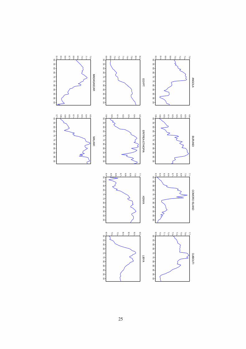
logs (see figures 2 and 3). Moreover, output differentials are defined with respect to
the corresponding panel average.
Before implementing the unit root tests, we first look at the shape of the regional
distribution of outcomes within the COMESA. This exercise must gives us an idea
11BN (2004) also consider the case when there are more than one common factors (r > 1) from a
sequential procedure. In our study, we find only one common factor.12See Maddison (2003) for a discussion on the Geary-Khamis approach.13Ethiopia and Eritrea are added into one item Eritrea–Ethiopia.
12

on the potential presence of a multiple equilibria configuration. So, we report in Fig-
ure (1) the distribution of real per capita GDP (in logs) across the set of Eastern and
Southern African countries in 1960, 1980 and 2003. The plotted distributions are ker-
nel density estimates based on a Epanechnikov kernel.14 Then, a number of features
can be put forward. Firstly, the distribution did not change obviously during the last
five decades. Interestingly, this latter corresponds to the so-called "twin peaks" phe-
nomenon highlighted by Quah (1993), Jones (1997) and Beaudry et al. (2005). This
result seems to indicate that there is a bimodal distribution of output per capita leading
to two different modes of convergence into the COMESA. Secondly, we observe that
the first hump has shifted toward the left, indicating that a large part of countries are
converging to a deteriorating average outcome per capita. Moreover, the distribution
around the second hump is wider, suggesting a more and more ambiguous evidence
about convergence between the richest economies of the sample.
However, one drawback in Figure (1) is that individual countries can not be
isolated. So, in addition, we check if there are some exogenous15 convergent clubs
in the COMESA by analyzing some groups of COMESA countries. Note that the
notions of “convergence clubs” and “poverty or underdevelopment trap” are closely
linked. The first one relies on the idea that, although no absolute or conditional
convergence16 of economies toward a similar path of development is observable (there
is no global convergence), one still might observe some local convergence properties.
Similarly, there are convergence clubs if countries have globally heterogeneous growth
dynamics, but can be grouped in subsets that show homogeneous growth patterns.
Then, all countries belonging to one specific club are characterized by the same kind
of equilibrium within a multiple equilibrium setting (Berthélemy, 2005). Finally,
economies concerned by the lower equilibrium are in a long-lasting situation of
poverty trap. Evidence on poverty traps has been extensively discussed in the empirical
14All distributions are expressed as deviations from the given year’s mean. Moreover, we use
a bandwidth parameter given by h = 0.9kN−(1/5)min(s,(IQR)/1.34) where N is the number of
observations, s is the standard deviation, IQR is the interquartile range of the series, and k is a canonical
bandwidth-transformation.15See Beine and Jean-Pierre (2000) for an endogenous determination of the convergence clubs.16Precise that one must not make the confusion between the notions of "conditional convergence"
and "convergence clubs". Indeed, although the former one implies that economies converge to different
steady states, their growth processes can be represented using the same model contrary to the latter
concept. Then, following the words of Berthélemy (2005), "instead of proper multiple equilibria, one
would observe multiple variants of the same equilibrium, parameterized by the conditioning variables"
(Berthélemy, 2005, p.6).
13

Figure 1: Cross-country real per capita GDP distribution: 1950, 1980 and 2003
literature (Abramovitz, 1986; Baumol, 1986; Quah, 1997; Hausmann et al., 2004;
among others), and several sources of multiple equilibria have been put forward
(Berthélemy, 2005).17
In this article, we focused on the two following criteria (Table 1):
(i) the degree of economic development: The importance of economic development
(human capital, health, infrastructure, . . . ) have been demonstrated since a long
time ago (Gillis et al., 1987). Recently, the New Growth Theory insisted on
the crucial impact of the initial development conditions for economic growth
and convergence. For that purpose, we first focused on the classification of
the United Nations Development Program based on the Human Development
Indicator (hereafter, HDI). This indicator has the decisive advantage of including
two main sources of poverty trap, namely education and income per capita
levels (Durlauf and Johnson, 1995). Otherwise, we fixed a threshold value
of 0.6 so that we have two homogeneous groups: the High/Moderate Human
Development Indicator (hereafter, HMHDI) group and the relatively Low
17The author gives a good survey on the different theoretical insights about the generating factors
of multiple equilibria. Globally, one can mention (i) the process of capital accumulation, (ii) the
role of human capital, and particularly of education, (iii) productivity gains related to research and
development activities, (iv) the financial deepening process, (v) the output diversification process, and
(vi) the institutional framework (corruption and civil strife).
14

Human Development Indicator (hereafter, LHDI). We also retained the concept
of Less Developed Countries (hereafter, LDC) established by the United Nation
Conference on Trade and Development.18
(ii) the economic diversification (Feenstra et al., 1999), and more precisely here the
importance of oil in the production and the export structures: Most countries
belonging to COMESA have a poor diversified export base. Some of them
strongly depend on oil resources. One more time, we can build two groups
from this criterion: the oil countries group, that is to say those which belong to
the African Petroleum Producers Association (hereafter, APPA) and the non-oil
countries group (hereafter, Non-APPA).
Table 1: COMESA’s countries shaped following three criteria.
Regional integration agreement Country
COMESA Angola, Burundi, Comoros, Democratic Republic of Congo, Djibouti, Egypt,
Eritrea–Ethiopia, Kenya, Libya, Madagascar, Malawi, Mauritius, Rwanda,
Seychelles, Sudan, Swaziland, Tanzania, Uganda, Zambia, Zimbabwe
Economic development criterion Country
HMIDH Egypt, Libya, Mauritius, Seychelles
LHDI Angola, Burundi, D.R. Congo, Comoros, Djibouti, Eritrea–Ethiopia, Kenya,
Madagascar, Malawi, Rwanda, Sudan, Swaziland, Tanzania, Uganda,
Zambia, Zimbabwe
LDC Angola, Burundi, D.R. Congo, Comoros, Djibouti, Eritrea–Ethiopia,
Madagascar, Malawi, Rwanda, Sudan, Tanzania, Uganda, Zambia
Economic structure criterion Country
APPA Angola, D.R. Congo, Egypt, Libya, Sudan
Non-APPA Burundi, Comoros, Djibouti, Eritrea–Ethiopia, Kenya, Madagascar, Malawi,
Mauritius, Rwanda, Seychelles, Swaziland, Tanzania, Uganda, Zambia, Zimbabwe
18Note that a country is classified as a LDC if it meets three criteria based on: (i) low-income (three-
year average GNI per capita of less than US $750, which must exceed $900 to leave the list), (ii)
human resource weakness (based on indicators of nutrition, health, education and adult literacy) and (iii)
economic vulnerability (based on instability of agricultural production, instability of exports of goods
and services, economic importance of non-traditional activities, merchandise export concentration, and
handicap of economic smallness, and the percentage of population displaced by natural disasters).
15

4.2 Panel unit root tests
The adopted strategy to test for income convergence is straightforward. Firstly, for
each group, we apply panel unit root tests with no fixed individual effects in order
to check if an absolute convergence process is present in the sample considered.
Secondly, for the groups where the null of unit root can not be rejected, the same
panel unit root tests but with fixed individual effects are implemented to pin downs a
possible conditional convergence dynamics. Finally, if the unit root hypothesis always
holds, then we consider that the group is characterized by stochastic divergence. We
apply the following panel unit root tests: (i) with no individual effects suggested by
Levin et al. (2002) [LLC1, t∗ρ], and (ii) with individual effects by Levin et al. (2002)
[LLC2, t∗ρ], Im et al. (2003) [IPS, tbarNT ] and Bai and Ng (2004) [BNc and BNi for
common factors (ADFcF
) and idiosyncratic shocks (Pcε ), respectively.].
Table 2 reports the panel unit root tests for the COMESA as well as from other
income references (an African average and a World average). The results shows no
evidence of absolute and conditional convergence. However, note that this finding of
no convergence process for the trade arrangement criterion does not reveal that regional
integration is not an efficient strategy to make developing countries to converge. In
our point of view, this result just tells us that the ongoing process of integration is
not adapted in this part of Africa. In accordance with the so-called Spaghetti Bowl
effect of Bhagwati et al. (1998), the high number of trade agreements in Eastern and
Southern Africa contributes to this bad performance in terms of income convergence.19
Moreover, although this agreement was officially created since 1981, the economic
cooperation process within COMESA is relatively recent in the extent that the free
trade area and the customs union were established in 2000 and 2009, respectively. In
addition, at date just a small number of countries does participate to these latter.
Table 3 displays the outcomes resulting from the panel unit root tests for the
different convergence clubs presented in Table 1. If we use the economic structure
criterion, there is no clubs convergence. The null of a unit root is not rejected by all
the tests both for the absolute and conditional convergence hypothesis whatever the
group considered (APPA, Non-APPA). Moreover, taking into account the presence of
cross-sectional dependence does not change the results. The reject of the convergence
19All COMESA countries belong to at least another African trade arrangement. More precisely, five
RIAs are concerned, namely the Indian Ocean Commission (IOC), the East African Community (EAC),
the Southern African Development Community (SADC), the Economic Community of Central African
States (ECCAS), the Arab Maghreb Union (AMU), Intergovernmental Authority for Development
(IGAD) and the Cross-Border Initiative (CBI).
16

Table 2: Panel unit root tests – COMESA – 1950–2003.
References LLC1 LLC2 IPS BNc BNi
COMESA average 3.82(0.99)
1.43(0.92)
3.04(0.99)
−1.55(0.50)
32.48(0.80)
African average 3.38(0.99)
2.31(0.99)
2.62(0.99)
−0.34(0.92)
30.90(0.85)
World average 8.88(1.00)
3.46(0.99)
6.22(1.00)
1.20(0.99)
41.13(0.42)
∗ and ∗∗ Significant at the 5% and 10% level, respectively. The p-values are given in parentheses. LLC1 and LLC2
denote the Levin, Liu and Chin (2002) panel unit root test with no individual effects and with individual effects
respectively. IPS denotes the Im, Pesaran and Shin (2003) unit root test with individual unit root processes. BNc
and BNi denote the Bai and Ng (2004) second-generation unit root test for common factors (ADFcF
) and idiosyncratic
shocks (Pcε ), respectively. Note that all these three last tests are done with individual effects.
for these two groups is not very surprising. The discrimination by the oil criterion
is not sufficient to constitute homogeneous groups in the case of the COMESA.
Several members reveal a production structure more diversified as for instance Egypt,
Mauritius or Seychelles.
The grouping by the economic development criterion provides the more interesting
findings. Two out of three groups are associated with an absolute income convergence
trend. In effect, the null hypothesis of a unit root can be rejected at the 5% and
10% level for the LDC and HMHDI groups, respectively, from the panel unit root
test with no individual effects LLC1. This result implies that the level of per capita
income of the poor countries in these groups catch-up with the one of the rich ones.
Concerning the last one, the LHDI group, a divergent process seems to characterize
the data, i.e. this group do not converge. That is not very surprising because of the
strong economic development disparities which are still present in this group. Indeed,
some countries as Zimbabwe, Kenya or Swaziland reveal HDI performances close to
the upper limit of 0.6. Although their economic development levels stay relatively low,
they do undoubtedly better than the fourteen other countries.
Thus, our work allows us to strongly support the theoretical insight. Economic
development is crucial for improving the growth performances of an economy.
This conjecture is more evident for the COMESA. Countries with good economic
development conditions (Mauritius, Seychelles, Libya, Egypt) show a catching
up process towards a high income average. But, countries with bad economic
development conditions, i.e. sixteen out of twenty economies, converge towards a
low income average. Thus, we can conclude from this study that there is an income
17

convergence process towards the bottom within the COMESA. Indeed, except for four
countries, all the members of this regional agreement are locked into the poverty trap.
Note that our results are conformed to the insights of the well-known “twin peaks”
literature (Jones, 1997; Beaudry et al., 2005). This latter revealed that the shape of
distribution of output per capita across countries has changed considerably over time.
Particularly, since the beginning of the eighties, a clear twin-peaked shape had emerged
with a cluster of rich countries and a cluster of poor countries. This structure seems to
also characterize the COMESA area.20
Table 3: Panel unit root tests – Convergence clubs – 1950–2003.
Groups LLC1 LLC2 IPS BNc BNi
Economic structure criterion
APPA −0.15(0.44)
−0.61(0.27)
0.29(0.61)
−1.29(0.63)
2.56(0.98)
NON-APPA 4.34(1.00)
3.49(0.99)
5.83(1.00)
0.37(0.98)
37.45(0.16)
Economic development criterion
LHDI −0.32(0.38)
1.42(0.92)
2.70(0.99)
−1.67(0.45)
27.83(0.68)
HMHDI −1.42∗∗(0.08)
– – – –
LDC −2.45∗(0.01)
– – – –
∗ and ∗∗ Significant at the 5% and 10% level, respectively. The p-values are given in parentheses. LLC1 and LLC2
denote the Levin, Liu and Chin (2002) panel unit root test with no individual effects and with individual effects,
respectively. IPS denotes the Im, Pesaran and Shin (2003) unit root test with individual unit root processes. BNc
and BNi denote the Bai and Ng (2004) second-generation unit root test for common factors (ADFcF
) and idiosyncratic
shocks (Pcε ), respectively. Note that all these three last tests are done with individual effects.
5 Conclusion
In this paper, we proposed to detect the possibility of stochastic convergence of real
per capita GDP for a set of Eastern and Southern African countries, all members of the
COMESA’s trade agreement. Using the panel unit-root tests developed by Levin et al.
(2002), Im et al. (2003) and Bai and Ng (2004), our results rejected the presence of
stochastic convergence for the whole COMESA. Contrary to the conceptual conclusion
20We have obtained the same results by using panel unit root tests that allow for structural breaks
(Carrion-i-Silvestre et al., 2005) and panel unit root tests that allow changes in persistence (Costantini and
Gutierrez, 2007). Note that the detected breaks are not associated with the establishment of COMESA.
18

of Venables (2003) about South-South integration, the lack of convergence in our case
does not imply that regional integration does not stimulate the setting up of a catching
up process. Actually, in our point of view, this bad performance results from the so-
called “Spaghetti Bowl” effect of Bhagwati et al. (1998). Thus, this region needs a
strategy based on a rationalization of the number of trade agreements before deepening
the trade and financial relations between the different economies.
However, in the extent that most COMESA countries are largely heterogeneous,
we tried to put forward the potential existence of convergence clubs within the trade
agreement by two criteria, namely (i) the economic structure (dependence from oil
production) and (ii) the degree of global economic development. Two main findings
emerged from the results. Firstly, no evidence of stochastic absolute and conditional
income convergence holds for the economic structure criteria. Secondly, the testing
procedures highlighted strong support for absolute income convergence for two groups
(HMHDI, LDC) belonging to the economic development criterion. This result led us
to conclude that a convergence process towards the bottom is at work for the COMESA
members, except for the most four developed countries, that is Mauritius, Seychelles,
Libya and Egypt. This result corroborates the findings of the New Growth Theories
in the extent that initial economic development conditions determine the long-run
economic growth processes. A related outcome is the necessary intervention of both
local governments and international institutions to create a climate of sustainable
development and get these under-development economies out of the poverty trap.
Indeed, a poor country can not escape from poverty without the implementation of
policy initiatives to change initial conditions in such a way that this country could jump
from its low level but stable initial equilibrium to another stable one but characterized
by a higher level of income.21
21A review for the political strategies available to lift a poor economy out of its poverty trap is given
by Berthélemy (2005).
19

References
[1] Bai J., Ng S. (2002), "Determining the number of factors in approximate factor
models", Econometrica, 70, 191-221.
[2] Bai J., Ng S. (2004), "A PANIC attack on unit roots and cointegration",
Econometrica, 72, 1127-1178.
[3] Baltagi B.H., Kao C. (2000), "Nonstationary panels, cointegration in panels
and dynamic panels: A survey", in Advances in Econometrics, Elsevier, North
Holland.
[4] Banerjee A. (1999), "Panel data unit root and cointegration: An Overview",
Oxford Bulletin of Economics and Statistics, Special Issue, 607-629.
[5] Banerjee A., Marcellino M., Osbat C. (2005), "Testing for PPP: Should we use
panel methods?", Empirical Economics, 30, 77-91.
[6] Banerjee A., Lumsdaine R.L., Stock J.H. (1992), "Recursive and sequential test
of the unit-root and trend-break hypothesis: Theory and international evidence",
Journal of Business and Economics Statistics, 10, 271-287.
[7] Barro R.J., Sala-i-Martin X. (1991), "Convergence across states and regions",
Brookings Papers on Economic Activity, 1, 107-158.
[8] Barro R.J., Sala-i-Martin X. (1992), "Convergence", Journal of Political
Economy, 100, 223-251.
[9] Baumol W. J. (1986), "Productivity growth, convergence and welfare: What the
long run data show", American Economic Review, 76, 1072-1085.
[10] Beaudry P., Collard F., Green D.A. (2005), "Changes in the world distribution of
output per worker, 1960-1998: how a standard decomposition tells an unorthodox
story", The review of Economics and Statistics, 87, 741-753.
[11] Beine M., Jean-Pierre Ph. (2000), "L’apport des tests de racine unitaire en
panel à l’identification des clubs de convergence", in Beine M., Docquier F.
(eds), Croissance et convergence économiques des régions, De Boeck University,
Bruxelles, 235-260.
[12] Bernard A., Durlauf S. (1995) "Convergence in international output", Journal of
Applied Econometrics, 10, 97-108.
20

[13] Bernard A., Durlauf S. (1996) "Interpreting tests of the convergence hypothesis",
Journal of Econometrics, 71, 161-173.
[14] Berthélemy J.-C. (2005) "Convergence clubs and multiple equilibria: how did
emerging economies manage to escape the under-development trap?", Review of
Economics and Development, 20(1), 5-44.
[15] Bertocchi G., Canova F. (2002), "Did colonization matter for growth? An
empirical exploration into the historical causes of Africa’s underdevelopment",
European Economic Review, 46, 1851-1873.
[16] Bhagwati J., Greenaway D., Panagariya A. (1998), "Trading preferentially:
Theory and policy", The Economic Journal, 108, 1128-1148, July.
[17] Block S.A. (2001), "Does Africa grow differently?", Journal of Development
Economics, 65, 443-467.
[18] Bloom D.E., Sachs J.D. (1998), "Geography, demography, and economic growth
in Africa", Brookings Papers on Economics, 207-295.
[19] Breitung J., Das S. (2008), "Testing for unit roots in panels with a factor
structure", Econometric Theory, 24, 88-108.
[20] Breitung J., Pesaran M. (2008), "Unit roots and cointegration in panels", in
Matyas L. and Sevestre P. (eds.), The Econometrics of Panel Data, New Jersey:
Springer-Verlag.
[21] Carmignani F. (2006), "The road to regional integration in Africa:
Macroeconomic convergence and performance in COMESA", Journal of African
Economies, 15, 212-250.
[22] Carmignani F. (2007), "A note on income converge effects in regional integration
agreements", Economics Letters, 94, 361-366.
[23] Carrion-i-Silvestre J-L., del Barrio-Castro T., Lopez-Bazo E. (2005), "Breaking
the panels: An application to the GDP per capita", Econometrics Journal, 8,
159-175.
[24] Choi I. (2001), "Unit root tests for panel data", Journal of International Money
and Finance, 20, 249-272.
[25] Choi I. (2006), "Nonstationary panels", in Mills T.C., Patterson K. (eds.),
Palgrave Handbook of Econometrics: Econometric Theory, Palgrave Macmillan.
21
[26] Collier P., Gunning J.W. (1999), "Why has Africa grown slowly?", Journal of
Economic Perspectives, 13, 3-22.
[27] Costantini M., Gutierrez L. (2007), "Simple panel unit root tests to detect changes
in persistence", Economics Letters, 96, 363-368.
[28] Cuñado J., Pérez de Gracia F. (2006), "Real convergence in Africa in the second-
half of the 20th century", Journal of Economics and Business, 58, 153-167.
[29] de Silva S., Hadri K., Tremayne A.R. (2009), "Panel unit root tests in the presence
of cross-sectional dependence: finite sample performance and an application",
Econometrics Journal, 12, 340-366.
[30] Easterly W., Levine R. (1997), "Africa’s growth tragedy: Policies and ethnic
divisions", Quarterly Journal of Economics, 112, 1203-1250.
[31] Evans P. (1996), "Using cross-country variances to evaluate growth theories",
Journal of Economic Dynamics and Control, 20, 1027-1049.
[32] Evans P., Karras, G. (1996), "Convergence revisited", Journal of Monetary
Economics, 37, 249-265.
[33] Feenstra R.C., Dorsati M., Yang T.-H., Liang C.-L. (1999), "Testing endogeneous
growth in South Korea and Taiwan", Journal of Development Economics, 60,
317-341.
[34] Gengenbach C., Palm F.C., Urbain J-P. (2010), "Panel unit root tests in the
presence of cross-sectional dependencies: Comparison and implications for
modelling", Econometric Reviews, forthcoming.
[35] Guetat I., Serranito F.. (2007), "Income convergence within the MENA countries:
A panel unit root approach", The Quaterly Review of Economics and Finance, 46,
685-706.
[36] Haldrup N., Jansson M. (2006), "Improving size and power in unit root
testing", in Mills T.C., Patterson K. (eds.), Palgrave Handbook of Econometrics:
Econometric Theory, Palgrave Macmillan.
[37] Hall A., (1994), "Testing for a unit root in time series with pretest data-based
model selection", Journal of Business and Economic Statistics, 12, 461-70.
22

[38] Hlouskova J., Wagner, M. (2006), "The performance of panel unit root and
stationarity tests: Results from a large scale simulation study", Econometric
Reviews, 25, 85-116.
[39] Hurlin C. (2010), "What would Nelson and Plosser find had they used panel unit
root tests?", Applied Economics, forthcoming.
[40] Im K.S., Pesaran M.H., Shin Y. (2003), "Testing for unit roots in heterogeneous
panels", Journal of Econometrics, 115, 53-74.
[41] Islam N. (2003), "What have we learnt from the convergence debate?", Journal
of Economic Survey, 17, 309-362.
[42] Jones C.I. (1997), "On the evolution of the world income distribution", Journal
of Economic Perspectives, 11, 19-36.
[43] Kraay A., Raddatz C. (2005), "Poverty traps, aid and growth", World Bank
background paper for the 2005 Global Monitoring Report.
[44] Levin A., Lin C.F., Chu. C.S.J. (2002), "Unit root test in panel data: Asymptotic
and finite sample properties", Journal of Econometrics, 108, 1-24.
[45] Lima Marcos A.M., Resende M. (2007), "Convergence of per capita GDP in
Brazil: An empirical note", Applied Economics Letters, 14, 333-335.
[46] MacKinnon J.G. (1991), Critical values for cointegration tests. In: Engle,
R.F., Granger, C.W. (Eds.), Long-Run Economic Relationship: Readings in
Cointegration. Oxford Press, Oxford.
[47] MacKinnon J.G. (1994), "Approximate asymptotic distribution functions for
unit-root and cointegration", Journal of Business and Economic Statistics, 12,
167-176.
[48] Maddala G.S., Wu S. (1999), "A comparative study of unit root tests with panel
data and a new simple test", Oxford Bulletin of Economics and Statistics, 61,
631-652.
[49] Maddison A. (2003), The World Economy: A Millennial Perspective, Develop-
ment Center for the OECD, Paris.
[50] McCoskey S.K. (2002), "Convergence in Sub-Saharan Africa: A nonstationary
panel data approach", Applied Economics, 34, 819-829.
23

[51] McCoskey S.K., Kao C. (1998), "A residual-based test of the null of cointegration
in panel data", Econometric Reviews, 17, 57-84.
[52] Paap R., Franses P.H., van Dijk D. (2005), "Does Africa grow slower than
Asia, Latin America and the Middle East? Evidence from a new data-based
classification method", Journal of Development Economics, 77, 553-570.
[53] Quah D. (1993), "Galton’s fallacy and tests of the convergence hypothesis",
Scandinavian Journal of Economics, 95, 427-443.
[54] Quah D. (1996), "Empirics for economic growth and convergence", European
Economic Review, 40, 1353-1375.
[55] Quah D. (1997), "Empirics for growth and distribution: stratification, polariza-
tion, and convergence clubs", Journal of Economic Growth, 2, 27-59.
[56] Romer P. (1986), "Increasing returns and long-run growth", Journal of Political
Economy, 94, 1002-1037.
[57] Romer P. (1990), "Endogenous technical change", Journal of Political Economy,
98, 71-102.
[58] Solow R. (1956), "A contribution to the theory of economic growth", Quarterly
Journal of Economics, 70, 65-94.
[59] Strauss J., Yigit T. (2003), "Shortfalls of panel unit root testing", Economics
Letters, 81, 309-313.
[60] Venables J. (2003), "Winners and losers from regional integration agreements",
Economic Journal, 113, 747-761.
24
6.2
6.4
6.6
6.8
7.0
7.2
7.4
7.6
50
55
60
65
70
75
80
85
90
95
00
AN
GO
LA
5.8
5.9
6.0
6.1
6.2
6.3
6.4
6.5
6.6
50
55
60
65
70
75
80
85
90
95
00
BU
RU
ND
I
6.3
6.4
6.5
6.6
6.7
6.8
6.9
7.0
7.1
50
55
60
65
70
75
80
85
90
95
00
CO
MO
RO
ISLA
ND
6.9
7.0
7.1
7.2
7.3
7.4
7.5
7.6
7.7
50
55
60
65
70
75
80
85
90
95
00
DJIB
OU
TI
6.6
6.8
7.0
7.2
7.4
7.6
7.8
8.0
8.2
50
55
60
65
70
75
80
85
90
95
00
EG
YP
T
5.9
6.0
6.1
6.2
6.3
6.4
6.5
50
55
60
65
70
75
80
85
90
95
00
ER
ITR
EA
-ET
HIO
PIA
6.4
6.5
6.6
6.7
6.8
6.9
7.0
7.1
50
55
60
65
70
75
80
85
90
95
00
KE
NY
A
6.5
7.0
7.5
8.0
8.5
9.0
9.5
50
55
60
65
70
75
80
85
90
95
00
LIB
YA
6.4
6.5
6.6
6.7
6.8
6.9
7.0
7.1
7.2
50
55
60
65
70
75
80
85
90
95
00
MA
DA
GA
SC
AR
5.7
5.8
5.9
6.0
6.1
6.2
6.3
6.4
6.5
50
55
60
65
70
75
80
85
90
95
00
MA
LA
WI
25

7.6
8.0
8.4
8.8
9.2
9.6
50
55
60
65
70
75
80
85
90
95
00
MA
UR
ITIU
S
6.0
6.2
6.4
6.6
6.8
7.0
50
55
60
65
70
75
80
85
90
95
00
RW
AN
DA
7.4
7.6
7.8
8.0
8.2
8.4
8.6
8.8
9.0
50
55
60
65
70
75
80
85
90
95
00
SE
YC
HE
LLE
S
6.6
6.7
6.8
6.9
7.0
7.1
50
55
60
65
70
75
80
85
90
95
00
SU
DA
N
6.4
6.6
6.8
7.0
7.2
7.4
7.6
7.8
8.0
50
55
60
65
70
75
80
85
90
95
00
SW
AZ
ILA
ND
6.0
6.1
6.2
6.3
6.4
6.5
50
55
60
65
70
75
80
85
90
95
00
TA
NZ
AN
IA
6.2
6.3
6.4
6.5
6.6
6.7
6.8
50
55
60
65
70
75
80
85
90
95
00
UG
AN
DA
5.2
5.4
5.6
5.8
6.0
6.2
6.4
6.6
6.8
50
55
60
65
70
75
80
85
90
95
00
ZA
IRE
6.4
6.5
6.6
6.7
6.8
6.9
7.0
7.1
50
55
60
65
70
75
80
85
90
95
00
ZA
MB
IA
6.5
6.6
6.7
6.8
6.9
7.0
7.1
7.2
7.3
50
55
60
65
70
75
80
85
90
95
00
ZIM
BA
BW
E
26

27