Convergence of a mountain pass type algorithm for strongly ... · Convergence of a mountain pass type algorithm for strongly indeﬁnite ... from the National Bank of Belgium and

Convergence of a mountain pass type algorithmfor strongly indefinite problems and systems

Grumiau Christopher, Troestler Christophe

Abstract. For a functional E and a peak selection that picks up a global maximum ofE on varying cones, we study the convergence up to a subsequence to a critical pointof the sequence generated by a mountain pass type algorithm. Moreover, by carefullychoosing stepsizes, we establish the convergence of the whole sequence under a “local-ization” assumption on the critical point. We illustrate our results with two problems:an indefinite Schrödinger equation and a superlinear Schrödinger system.

Mathematics Subject Classification (2000). Primary: 35J20, Secondary: 58E05,58E30, 35B38.Keywords. Mountain pass algorithm, minimax, steepest descent method, Schrödingerequation, spectral gap, strongly indefinite functional, ground state solutions, Neharimanifold, systems.

1. IntroductionLet us consider H a Hilbert space with inner product 〈·|·〉 and norm ‖·‖, and a functionalE ∈ C 1(H ;R). In this work, we develop a provably convergent “general” mountain passtype algorithm to approximate saddle points of E , with a Morse index possibly larger thanone. The pioneer work in this direction is due to Y. S. Choi and P. J. McKenna [4] whoproposed a constrained steepest descent method to compute saddle points with one “de-scent direction” (such as a Mountain Pass solution). A proof of convergence of a variantof that algorithm was later given by Y. Li and J. Zhou in [10, 11]. To briefly describe it,let us fix a closed subspace E of H and ϕ a continuous E⊥-peak selection, i.e. ϕ(u) isthe location of a maximum of E on E⊕R+u := e+ ty | e ∈ E, t > 0 for any u ∈H \Eand ϕ is constant on E⊕R+u. As it will be convenient in the rest of the paper that ϕ isnot solely defined on a unit sphere, we present here a slightly different version [21].

The authors are partially supported by a grant from the National Bank of Belgium and by the program “Qualita-tive study of solutions of variational elliptic partial differerential equations. Symmetries, bifurcations, singular-ities, multiplicity and numerics” of the FNRS, project 2.4.550.10.F of the Fonds de la Recherche FondamentaleCollective.

arX

iv:1

301.

1456

v1 [

mat

h.A

P] 8

Jan

201

3

2 Ch. Grumiau, Ch. Troestler

Algorithm 1.1 (Mountain Pass Algorithm). (i) Choose u0 ∈ Ranϕ , ε > 0 and n←0;

(ii) if ‖∇E (un)‖6 ε then stop;else compute

un+1 = ϕ

(un− sn

∇E (un)

‖∇E (un)‖

),

for some sn ∈ S(un)⊆ (0,+∞) where S(un) is a set of “admissible stepsizes” chosenso that at least the following inequality holds:

E (un+1)−E (un)<− 12 sn‖∇E (un)‖;

(iii) let n← n+1 and go to step 2.

Y. Li and J. Zhou proved that (un) converges to a nontrivial critical point of Eup to a subsequence. The proof of convergence is performed in the space H to ensurethat the rate of convergence for the discretized problem does not deteriorate when theapproximating subspace becomes finer. The original goal of the authors for introducing Ewas to try to obtain multiple critical points by taking E as the linear subspace generated bypreviously found solutions which the algorithm must try to avoid. The proof is performedin two steps. First, they show that sn exists and that E decreases along (un)n∈N. This steprelies on the following deformation lemma.

Lemma 1.2. If ϕ is continuous, u0 ∈ Ranϕ , u0 /∈ E, ∇E (u0) 6= 0, then there exists s0 > 0such that

∀s ∈ (0,s0], E(ϕ(us)

)−E (u0)<− 1

2 s‖∇E (u0)‖,where

us := u0− s∇E (u0)

‖∇E (u0)‖.

The second step consists in proving, under some traditional assumptions on ϕ , thata subsequence of (un) converges. For this, it is essential to show that the stepsize sn con-trols the distance between un and un+1 and that sn is chosen in such a way that it is closeto 0 only when “mandated” by the functional. Let us remark that the choice of ϕ is verysensitive. Indeed, to seek sign-changing critical points, the modified mountain pass algo-rithm was introduced by J. M. Neuberger [14] (see also [7]). He considers algorithm 1.1above and only modifies the projection ϕ into a “sign-changing peak selection” ϕN whichis a map defined from the set of sign-changing functions of H \ 0 to H \ 0 suchthat, for any u, E

(ϕN(u)

)> 0 and ϕN(u) is a maximum of E on R+u+⊕R+u− where

u+(x) := max0,u(x) and u−(x) := min0,u(x). Although in practice it appears to con-verge to a nontrivial sign-changing critical point, its convergence has yet to be formallyproved.

In this paper, ϕ(u) is allowed to pick up a maximum point of E in an abstract coneCu and we are interested in giving assumptions on Cu which imply the convergence ofthe mountain pass algorithm. This work is partly motivated by the article [17] wherethe authors define the notion of “natural constraints” to seek nontrivial critical points offunctionals. Let us first make precise the peak selection ϕ that we use. We write intC

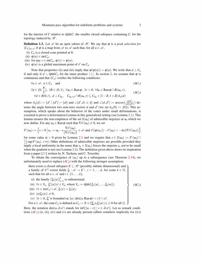
Mountain pass algorithm for indefinite problems and systems 3

for the interior of C relative to spanC, the smaller closed subspace containing C, for thetopology induced by H .

Definition 1.3. Let A be an open subset of H . We say that ϕ is a peak selection for(Cu)u∈A if ϕ is a map from A to A such that, for all u ∈A ,

(i) Cu is a closed cone pointed at 0;(ii) ϕ(u) ∈ intCu;

(iii) for any v ∈ intCu, ϕ(v) = ϕ(u);(iv) ϕ(u) is a global maximum point of E on Cu.

Note that properties (ii) and (iii) imply that ϕ(ϕ(u)) = ϕ(u). We write that d ⊥Cuif and only if d ⊥ spanCu for the inner product 〈·|·〉. In section 2, we assume that ϕ iscontinuous and that (Cu) verifies the following conditions:

∀u ∈A , u ∈Cu and (AC1)

∃γ ∈(0,

π

2), ∃δ ∈ (0,1), ∀u0 ∈ Ranϕ, ∃r > 0, ∀u0 ∈ Ranϕ ∩B(u0,r),

∀d ∈ B(0,r), d ⊥Cu0 , Cu0+d ∩B(u0,r)⊆Cu0 +[1−δ ,1+δ ]Aγ(d)(AC2)

where Aγ(d) := d′ | ‖d′‖ = ‖d‖ and ∠(d′,d) 6 γ and ∠(d,d′) := arccos( 〈d|d′〉‖d‖‖d′‖

)de-

notes the angle between two non-zero vectors d and d′ (we set Aγ(0) := 0). This as-sumption, which speaks about the behavior of the cones under small deformations, isessential to prove a deformation Lemma in this generalized setting (see Lemma 2.1). Thislemma ensures the non-emptiness of the set S(u0) of admissible stepsizes at u0 which wenow define. For any u0 ∈ Ranϕ such that ∇E (u0) 6= 0, we set

S∗(u0) :=

s> 0∣∣∣ us := u0−s

∇E (u0)

‖∇E (u0)‖∈A and E

(ϕ(us)

)−E (u0)<−αs‖∇E (u0)‖

for some value α > 0 given by Lemma 2.1 and we require that s ∈ S(u0) := S∗(u0)∩[ 1

2 supS∗(u0),+∞). Other definitions of admissible stepsizes are possible provided they

imply a local uniformity in the sense that sn ∈ S(un) forces the stepsize sn not to be smallwhen the gradient is not (see Lemma 2.4). The definition given above draws its inspirationfrom a paper [21] written by N. Tacheny and C. Troestler.

To obtain the convergence of (un) up to a subsequence (see Theorem 2.14), weunfortunately need to replace (AC2) with the following stronger assumption:

there exists a closed subspace E ⊆H (possibly infinite dimensional) anda family of C 1-vector fields ξi : A → E⊥, i = 1, . . . ,k, for some k ∈ N,such that for all u ∈A and i ∈ 1, . . . ,k,

(i) the family(ξi(u)

)ki=1 is orthonormal;

(ii) ∀v ∈Vu, ξ ′i (u)[v] ∈Vu, where Vu := spanξ1(u), . . . ,ξk(u);(iii) ∀v ∈ intCu∩A , ξi(v) = ξi(u);(iv) 〈u|ξi(u)〉 6= 0;(v) ∃r > 0, ξ ′i is bounded on u | dist(u,Ranϕ)< r∩A .

For u∈A , the cone Cu is defined as Cu := E⊕∑i tiξi(u) | ti > 0 for all i.

(AC3)

Here, the notation dist(u,∂A ) stands for inf‖u− v‖ | v ∈ ∂A . Let us remark condi-tions (AC3) (i), (ii), (iv) and (v) are already present (albeit somehow implicitly for (iv))


in [17] in the context of trivial C 1-subbundles intead of cones. The additional condi-tion (iii) is equivalent to ∀v ∈ intCu ∩A , Cv = Cu. This condition is rather natural torequire in view of property (iii) of the definition of peak selection. This “finite presenta-tion” of the cones is used in Lemma 2.8 to ensure that the stepsize sn controls the distancebetween un+1 and un.

As a particular case of (AC3), let us mention that we can work with a family ofcontinuous linear projectors (see Proposition 2.12). This case is an abstract formulationof the setting of [2, 3] where the convergence (up to a subsequence) of a mountain passtype algorithm for systems has been announced.

In Section 2.3, we are interested in the convergence of the whole sequence generatedby the Mountain Pass Algorithm. To that aim, we need to refine the definition of S∗ inorder to control E

(ϕ(un− s ∇un

‖∇un‖ ))

for any 0 < s < sn.In Section 3, we illustrate our method with two semi-linear problems. The first ap-

plication takes its inspiration from a paper due to A. Szulkin and T. Weth [20] in whichthe authors study the following Schrödinger problem

−∆u(x)+V (x)u(x) = |u(x)|p−2u(x), x ∈Ω,

u(x) = 0, x ∈ ∂Ω,(1)

where V : Ω→ R is such that 0 is in a spectral gap of −∆+V and 2 < p < 2∗ := 2NN−2

(+∞ when N = 2). They are interested in the existence of non-zero solutions on an openbounded domain Ω⊆ RN or on Ω = RN (in the latter case, V is assumed to be 1-periodicin each xi, i = 1, . . . ,N). Solutions to this equation are critical points of the indefinitefunctional

E : H → R : u 7→ 12

∫Ω

(|∇u(x)|2 +V (x)u(x)2) dx− 1

p

∫Ω

|u(x)|p dx, (2)

where H = H10 (Ω). The first proof of the existence of non-zero critical points for E

when −∆+V is not positive definite and Ω is an open bounded domain is due to P. H.Rabinowitz [18]. Recently, A. Szulkin and T. Weth proposed an alternative method [20]that also makes easier to deal with the lack of compactness that occurs when Ω = RN .Denoting E the negative eigenspace of −∆+V , they introduce the following nonlinearmap

ϕ : H \E→H : u 7→ ϕ(u)

where ϕ(u) is the point at which E reaches its maximum value on E⊕R+u. They provethat minimizing E on Ranϕ =

u ∈H \E

∣∣ ∂E (u)[v] = 0 for v = u and any v ∈ E

yields a non-zero solution with least energy. Notice that, here, E is used to deal with theindefiniteness of the problem and not to compute multiple critical points as in the papersof J. Zhou & al. [10, 11]. We will prove that our algorithm converges for this problem.The numerical solutions that we obtain lead to some conjectures on the symmetries ofground state solutions.


The second application is based on a paper by B. Noris and G. Verzini [17]. Theauthors study the superlinear Schrödinger system

−∆ui(x) = ∂iF(u1(x), . . . ,uk(x)

), x ∈Ω,

ui(x) = 0, x ∈ ∂Ω,i = 1, . . . ,k, (3)

where k ∈N. They require that Ω⊆RN is a bounded smooth domain and F ∈ C 2(Rk;R).Note that the system −∆ui = µiu3

i +ui ∑ j 6=i βi, ju2j where µi > 0 and βi, j = β j,i is a partic-

ular case of (3). Such type of nonlinearities have been studied due to their applications tononlinear optics and to Bose-Einstein condensation (see [6, 5, 8, 22]). Solutions to (3) arecritical points of the functional

E : H → R : u = (u1, . . . ,uk) 7→12

∫Ω

|∇u(x)|2 dx−∫

Ω

F(u)dx, (4)

where H = H10 (Ω;Rk). As already mentioned, B. Noris and G. Verzini [17] propose a

general method of “natural constraints”. Applied to the above problem, it goes as follows.Denote A := u ∈ H | ui 6= 0 for every i. To find a solution u = (u1, . . . ,uk) of (3)with ui 6= 0 for all i = 1, . . . ,k, they minimize E on the constraint N :=

u ∈ A

∣∣ ∀i =1, . . . ,k,

∫Ω|∇ui|2 dx=

∫Ω

∂iF(u)ui dx

. We will show that, under their assumptions, N =Ranϕ with ϕ being the peak selection

ϕ : A →A : u 7→ argmaxE (t1u1, . . . , tkuk)

∣∣ t1 > 0, . . . , tk > 0.

Again, we prove that our algorithm converges for this problem and some numerical ex-periments are performed.

2. Steepest descent method on varying cones2.1. Uniform deformation lemmaLet E : H → R be a C 1-functional defined on a Hilbert space H and A an open subsetof H . The following lemma is instrumental in proving the convergence of the algorithm.

Lemma 2.1 (Uniform deformation lemma). Let ϕ : A → A be a peak selection for(Cu)u∈A and u0 ∈ Ranϕ be such that ∇E (u0) 6= 0. Assume that ϕ is continuous at u0 andthat (AC1)–(AC2) hold. Then there exist s0 > 0 and r0 > 0 such that, for any s∈ (0,s0] andu0 ∈ B(u0,r0)∩Ranϕ , one has

• ∇E (u0) 6= 0,• us ∈A where us := u0− s ∇E (u0)

‖∇E (u0)‖and

• there exists some α > 0 solely depending on γ and δ given in assumption (AC2) suchthat

E(ϕ(us)

)−E (u0)<−αs‖∇E (u0)‖. (5)

Proof. Let u0 ∈ Ranϕ ⊆A and let us consider γ , δ and r given by the assumption (AC2)for u0. Since A is open, there exists ε1 > 0 such that for any u∈B(u0,ε1) and v∈B(u,ε1),one has u,v ∈A , ∇E (u) 6= 0, ∇E (v) 6= 0 and u,v ∈ B(u0,r).


For any u ∈ B(u0,ε1), let du :=−∇E (u)/‖∇E (u)‖. Then

∀u ∈ B(u0,ε1), ∀d ∈ Aγ(du), 〈∇E (u)|d〉6−cosγ ‖∇E (u)‖.

Let γ := 12 cosγ > 0. Taking ε1 smaller if necessary, we may assume that

∀u,v ∈ B(u0,ε1), ∀d ∈ Aγ(du), 〈∇E (v)|d〉<−γ‖∇E (u)‖.

Thus, on one hand, there exists ε2 > 0 such that, for any u ∈ B(u0,ε2), v ∈ B(u,ε2),d ∈ Aγ(du) and σ ∈ (0,ε2),

〈∇E (v+σd)|d〉<−γ‖∇E (u)‖.

For any u0 ∈ B(u0,ε2)∩Ranϕ , v ∈ Cu0 ∩B(u0,ε2), d ∈ Aγ(du0) and σ < ε2, the meanvalue theorem implies there exists a σ ∈ (0,σ) such that

E (v+σd)−E (u0)6 E (v+σd)−E (v) (6)

=⟨∇E (v+ σd)

∣∣σd⟩

<−γσ‖∇E (u0)‖, (7)

where the first inequality results from v ∈Cu0 and u0 = ϕ(u0) is a global maximum of Eon Cu0 .

On the other hand, by the continuity of ϕ at u0, there exist s0 ∈ (0,r) and ε3 ∈(0,minr, 1

3 ε2)

such that, for any u0 ∈ B(u0,ε3) and s ∈ [0,s0], one has ϕ(u0 + sdu0) ∈B(u0,minr, 1

3 ε2). Let us := u0 + sdu0 . If in addition u0 ∈ Ranϕ , one has du0 ⊥ spanCu0

(because u0 = ϕ(u0) ∈ intCu0 is a local maximum) and therefore one deduces from as-sumption (AC2) that

ϕ(us) ∈Cus ∩B(u0,r)⊆Cu0 +[1−δ ,1+δ ]Aγ(sdu0).

Thus, ϕ(us) = vs +Kssd∗s for some vs ∈ Cu0 , Ks ∈ [1− δ ,1+ δ ] and d∗s ∈ Aγ(du0). So,possibly taking s0 smaller, we get that Kss < 1

3 ε2 and vs = ϕ(us)−Kssd∗s ∈ B(u0,ε2).Using equation (7), we conclude that

E(ϕ(us)

)−E (u0) = E (vs +Kssd∗s )−E (u0)6−γ (1−δ )s‖∇E (u0)‖

for any u0 ∈ B(u0,ε3)∩Ranϕ and s ∈ (0,s0].

Remark 2.2. • Equation (6) is the unique place we use that ϕ(u) is a global maximumof E on Cu. This assumption can be weakened by only requiring that the neighbor-hood on which ϕ(u) achieves the maximum of E is locally uniform w.r.t. u:

∀u0 ∈ Ranϕ, ∃ρ > 0, ∀u ∈ Ranϕ ∩B(u0,ρ), E(ϕ(u)

)= max

v∈Cu∩B(u,ρ)E (v). (8)

This assumption allows the existence of multiple maximums points in Cu. It was notused in definition 1.3 for simplicity but also because, in the examples of section 3,ϕ(u) is a maximum on the whole Cu.• Let us also note that, if we are just interested in the inequality (5) at u0 (and not

for all u0 in a neighborhood of u0), we only need to require that ϕ(u) is a localmaximum of E on Cu.


• A careful reader may notice that we did not really use the fact that Cu is a conepointed at 0. However, if (Cu) was just a family of sets satisfying (AC1), (AC2), (8)and the fact that ϕ(u) ∈ intCu in a locally uniform way:

∀u0 ∈ Ranϕ, ∃ρ > 0, ∀u ∈ Ranϕ ∩B(u0,ρ), B(u,ρ)∩ spanCu ⊆Cu, (9)

then the cone Cu, defined as the closure of tv | t > 0 and v∈Cu, also satisfies (AC1),(AC2), (8) and ϕ(u) ∈ intCu. So very little is gained by not using cones, especiallybecause they are the natural structures encountered in our examples.

• As a consequence of the above deformation lemma, one can interpret Ranϕ assomewhat a natural constraint for E in the sense of [17]. More precisely, it im-plies that if u0 ∈ Ranϕ is a local minimum of E on Ranϕ then u0 is a critical pointof E on the whole space H .

2.2. Convergence up to a subsequenceIn this section, we first remark that it is possible to construct a sequence of stepsizes snsuch that the energy E decreases along the sequence (un)n∈N generated by algorithm 1.1.In the following, without loss of generality, we can assume that ∇E (un) 6= 0 for any n∈N(otherwise the algorithm finds a critical point in a finite number of steps).

Proposition 2.3. If sn > 0 verifies inequality (5) given in Lemma 2.1 for any n ∈ N, thenthe functional E decreases along the sequence (un)n∈N.

Proof. As ∇E (un) 6= 0, sn is well-defined by Lemma 2.1. By construction, we have

E (un+1)−E (un) = E

(ϕ(un− sn

∇E (un)

‖∇E (un)‖))−E (un)<−αsn‖∇E (un)‖< 0.

So, E (un+1)< E (un).

As explained in the introduction, we now consider the sets S∗(u0) and S(u0). Theset S∗(u0) is not empty as soon as u0 is not a critical point of E (thanks to the deformationlemma). Concerning the set S(u0), it is not-empty once E is bounded from below onRanϕ , an assumption that we will later make (see Theorem 2.10).

Lemma 2.4. If u0 ∈ Ranϕ , ∇E (u0) 6= 0 and ϕ is continuous at u0, then there exists anopen neighborhood V of u0 and s∗ > 0 such that S(u)⊆ [s∗,+∞) for any u ∈V ∩Ranϕ .

Proof. By the uniform deformation Lemma 2.1, there exists s0 > 0 and r0 > 0 such that,for any 0 < s6 s0 and u ∈ B(u0,r0)∩Ranϕ , we have us := u− s ∇E (u)

‖∇E (u)‖ ∈A , ∇E (u) 6= 0and

E(ϕ(us)

)−E (u)<−αs‖∇E (u)‖. (10)

In particular, for any u ∈ B(u0,r0)∩Ranϕ , s0 ∈ S∗(u). It follows that S(u)⊆ [ s02 ,+∞). It

suffices to take s∗ 6 s0/2.

Remark 2.5. To prove Lemma 2.4, let us remark that we could only use inequality (10) atu = u0 for s = s0 fixed. Indeed, by continuity, it directly implies that s0 ∈ S(u) for u closeto u0. However, to obtain Lemma 2.4 for S(u) (see section 2.3) instead of S(u), the fullstrength of the deformation lemma is needed.


From now on, we have to require condition (AC3). Let us first show it subsumes (AC2).

Lemma 2.6. Let (ξi)ki=1 be the family of vector fields given by (AC3) and assume (AC1)

holds. Then

∀u ∈A , ∀d ⊥Cu,k

∑i=1

⟨u∣∣ξi(u)

⟩·ξ ′i (u)[d] = d−

k

∑i=1

⟨u∣∣ξ ′i (u)[d]⟩ξi(u).

Proof. For any u ∈A , the fact that u ∈Cu ⊆ Vu and that (ξi)ki=1 is an orthonormal basis

of Vu imply u = ∑〈u|ξi(u)〉ξi(u). Differentiating in a direction d ∈H , yields

d =k

∑i=1〈d|ξi(u)〉 ξi(u)+

k

∑i=1〈u|ξ ′i (u)[d]〉ξi(u)+

k

∑i=1〈u|ξi(u)〉 ·ξ ′i (u)[d].

If d ⊥ spanCu, the first term vanishes. This completes the proof.

Proposition 2.7. Properties (AC1) and (AC3) imply (AC2).

Proof. Let δ ∈ (0,1) (property (AC2) will be satisfied whatever value is chosen). Simplegeometrical considerations show that there exists a γ ∈ (0,π/2) such that

B(d,δ‖d‖)⊆ [1−δ ,1+δ ]Aγ(d).

Let u0 ∈ Ranϕ . As u0 ∈ intCu0 , there exist α > 0 such that 〈u0|ξi(u0)〉 > α for all i.Using the continuity of ξi and ξ ′i at u0, we can choose r sufficiently small and a M > 0(depending only on u0) so that, for all u ∈ B(u0,r) and all i = 1, . . . ,k,

〈u|ξi(u)〉> α, ‖ξi(u)−ξi(u0)‖6 ε, ‖ξ ′i (u)‖6M, and ‖ξ ′i (u)−ξ′i (u0)‖6 ε,

where ε > 0 is a constant depending only on δ and u0 (to be chosen later).Let u0 ∈ B(u0,r) and d ∈ B(0,r) such that d ⊥Cu0 . Let w ∈Cu0+d ∩B(u0,r). One

can write w = e+∑ tiξi(u0 + d) for some e ∈ E and ti > 0. Let us start by noticing thatti = 〈w|ξi(u0 +d)〉. Therefore, recalling that ‖ξi‖= 1, one deduces∣∣ti−〈u0|ξi(u0)〉

∣∣6 ∣∣⟨w− u0∣∣ξi(u0 +d)

⟩∣∣+ ∣∣⟨u0∣∣ξi(u0 +d)−ξi(u0)

⟩∣∣6 ‖w− u0‖+‖u0‖‖ξi(u0 +d)−ξi(u0)‖6 2r+(‖u0‖+ r)ε. (11)

Provided that ε and r are chosen small enough, one can assume that 2r+(‖u0‖+ r)ε 6α/3. In particular, this implies ti > 2α/3 > 0.

Using the integral form of the mean value theorem, we get

w = e+k

∑i=1

tiξi(u0 +d) = e+k

∑i=1

tiξi(u0)+∫ 1

0

k

∑i=1

ti ξ′i (u0 + sd)[d]ds. (12)

The third term can be rewritten as follows:k

∑i=1〈u0|ξi(u0)〉ξ ′i (u0)[d]+

k

∑i=1

(ti−〈u0|ξi(u0)〉

)ξ′i (u0)[d]

+∫ 1

0

k

∑i=1

ti(ξ′i (u0 + sd)[d]−ξ

′i (u0)[d]

)ds =: d1 +d2 +d3.


Using Lemma 2.6 on d1, one can write equation (12) as

w = e+k

∑i=1

(ti−〈u0|ξ ′i (u0)[d]〉

)ξi(u0)+d +d2 +d3.

Since∣∣〈u0|ξ ′i (u0)[d]〉

∣∣6 ‖u0‖‖ξ ′i (u0)‖‖d‖6 (‖u0‖+ r)Mr, we can assume r was chosensmall enough so that this is smaller that α/3. Recalling that ti > 2α/3, one sees that thecoefficients of ξi(u0) are positive and therefore e+∑

(ti−〈u0|ξ ′i (u0)[d]〉

)ξi(u0) ∈Cu0 .

The proof is complete if we show that d + d2 + d3 ∈ B(d,δ‖d‖). Using (11), wededuce |ti| 6

∣∣ti−〈u0|ξi(u0)〉∣∣+‖u0‖ 6 2r+(‖u0‖+ r)(ε +1). Thus the following esti-

mates

‖d2‖6k

∑i=1

∣∣ti−〈u0|ξi(u0)〉∣∣‖ξ ′i (u0)‖‖d‖6 k

(2r+(‖u0‖+ r)ε

)M ‖d‖,

‖d3‖6k

∑i=1|ti| sup

s∈[0,1]‖ξ ′i (u0 + sd)−ξ

′i (u0)‖‖d‖6 k

(2r+(‖u0‖+ r)(ε +1)

)ε‖d‖,

show that ‖di‖ 6 12 δ‖d‖, i = 2,3, provided that the constants ε and r were chosen small

enough.

Lemma 2.8 is the second key element to prove the convergence up to a subsequence.

Lemma 2.8. Let ϕ be a peak selection for (Cu)u∈A which verifies conditions (AC1) and(AC3). Let (un)n∈N and (sn)n∈N be given by the generalized MPA (algorithm 1.1) withsn ∈ S(un) for all n. Let us assume that ϕ is continuous, Ranϕ ⊆A , and either

∃τ1, . . . ,τk ∈ (0,+∞), dist( k

∑i=1

τiξi(u)∣∣∣ u ∈ Ranϕ

,∂A

)> 0, (13a)

or

∀(vn)⊆ Ranϕ,

(E (vn)

)is bounded from above⇒ (vn) is bounded

and dimE < ∞.(13b)

If ∑+∞

n=0 sn <+∞ then (un)n∈N converges in A .

Proof. Let k be given by the assumption (AC3). For i = 1, . . . ,k, set vi,n := ξi(un), anddn :=− ∇E (un)

‖∇E (un)‖ . Let r be given by assumption (AC3) (v) and Ki be a bound for ξ ′i . DenoteK := maxi=1,...,k Ki.

By assumption (AC3) and as ϕ(un + sndn) ∈ intCun+sndn , we have

vi,n+1 = ξi(ϕ(un + sndn)

)= ξi(un + sndn)

for any n ∈ N. Let n∗ be large enough so that sn < r. Thus, for all n> n∗,

‖vi,n+1− vi,n‖6 K‖sndn‖= Ksn. (14)

Since ∑sn < +∞, it follows that for any i = 1, . . . ,k, (vi,n)n∈N is a Cauchy sequence andtherefore converges to, say, vi,∞.

Let us assume (13a) holds. Consider vn := ∑ki=1 τivi,n = ∑

ki=1 τiξi(un). It converges

and its limits belongs to A . Since ϕ(vn) = ϕ(un) = un and ϕ is continuous, the sequence(un)n∈N converges. Its limit lies in Ranϕ and thus in A .


If on the other hand (13b) holds, the fact that the sequence (E (un)) is decreasingimplies that (un) is bounded. Let (u′n) be a subsequence of (un). Since u′n ∈Cu′n , one canwrite u′n = e′n +∑

ki=1 t ′i,nξi(u′n) for some e′n ∈ E and t ′i,n ∈ (0,+∞). As (u′n) is bounded, so

are (e′n) and |t ′i,n| = |〈u′n|ξi(u′n)〉| 6 ‖u′n‖. So, up to subsequences, (e′n)n∈N and (t ′i,n)n∈Nconverge to, say, e′∞ and t ′i,∞. Thus u′n → u′∞ := e′∞ +∑ t ′i,∞vi,∞. Thanks to Ranϕ ⊆ A ,u′∞ ∈A . But then the continuity of ξi and ϕ imply

vi,∞ = ξi(u′∞) and u′n = ϕ(u′n)→ ϕ(u′∞). (15)

If the same reasoning is performed with another subsequence (u′′n), (15) implies thatξi(u′∞) = ξi(u′′∞) and therefore, in view of definition 1.3 (iii), ϕ(u′∞) = ϕ(u′′∞). As thelimit does not depend on the subsequence, the whole sequence (un) converges in A .

Remark 2.9. If we wanted to seek sign-changing solutions using the cones Cu :=R+u+⊕R+u− (as explained in the Introduction), then we would not be able to remove the projec-tion factors in the above computation of vi,n+1. This sheds some light on the difficulty ofproving the convergence of the Modified Mountain Pass Algorithm [14].

Theorem 2.10. Assume ϕ : A → A is a continuous peak selection s.t. Ranϕ ⊆ Aand the cones (Cu)u∈A verify the conditions (AC1), (AC3) and (13a) or (13b). Supposemoreover that E ∈ C 1(H ;R) satisfies the Palais-Smale condition in Ranϕ and thatinfu∈Ranϕ E (u)>−∞. Then the sequence (un)n∈N given by the generalized mountain passalgorithm 1.1 possesses a subsequence converging to a critical point of E in Ranϕ . Inaddition, all limit points of (un)n∈N are critical points of E .

Proof. Let us start by showing that(∇E (un)

)n∈N converges to zero up to a subsequence.

If not, we could assume there exist δ > 0 and n0 ∈N such that, for any n> n0, ‖∇E (un)‖>δ . Then, for any n> n0, the deformation lemma 2.1 implies

E (un+1)−E (un)6−αsnδ .

Thus, summing up,

limn→+∞

E (un)−E (un0) =+∞

∑n=n0

E (un+1)−E (un)6−δα

+∞

∑n=n0

sn.

As the left-hand side is a real number (E is bounded from below on Ranϕ and de-creasing along (un)n∈N), we have ∑

+∞

n=0 sn < +∞. So, by Lemma 2.8, un → u∗ ∈ A and‖∇E (u∗)‖> δ . By continuity of ϕ at u∗ ∈A , we obtain ϕ(u∗) = u∗ and, so, u∗ ∈ Ranϕ .By Lemma 2.4, there exists a neighborhood V of u∗ and s∗ > 0 such that S(u)⊆ [s∗,+∞)for any u ∈ V . Consequently, there exists n0 such that, for any n > n0, sn > s∗ whence∑+∞

n=0 sn does not converge, which is a contradiction.In conclusion, there exists a subsequence (unk)k∈N of (un)n∈N s.t. ‖∇E (unk)‖ → 0

when k→ +∞. As E satisfies the Palais-Smale condition, (unk)k∈N possesses a subse-quence converging to a critical point of E .

Concerning the second statement of the theorem, the argument is very similar. Let(unk)k∈N be a convergent subsequence and assume on the contrary that u := limk→∞ unk


is not a critical point of E . In that case, on one hand, there exists δ > 0 and k1 ∈ N suchthat, for any k > k1, ‖∇E (unk)‖> δ . By Lemma 2.1, we have

∀k > k1, E (unk+1)−E (unk)6−αδ snk .

On the other hand, as u ∈ Ranϕ , we have by Lemma 2.4 that

∃ s∗ > 0, ∃k2 ∈ N, ∀k > k2, sn > s∗.

So, for large k, E (unk+1)−E (unk)6−α

2 δ s∗, which is a contradiction because(E (un)

)n∈N

is a convergent sequence.

Remark 2.11. By previous remarks 2.2 and 2.5, we conclude that we could get the con-vergence up to a subsequence using the equation (5) only at u0. Thus, the uniform form ofLemma 2.1 is not required (and we could consider that ϕ(u) is a local maximum of ϕ onCu instead of a global maximum). Nevertheless, we have kept the uniform setting alongthe paper as it will be required in Section 2.3.

The following special case of (AC3) is important for the applications.

There exist a closed subspace E ⊆H (possibly infinite dimensional) andlinear continuous projectors Pi : H → E⊥, i = 1, . . . ,k, for some k ∈ N,such that• ∀ u ∈H , Pi(u)⊥ Pj(u) whenever i 6= j;• E⊕∑

ki=1 RanPi = H .

For all u ∈H , set Cu := E⊕

∑ tiPi(u)∣∣ ti > 0 for all i

.

(AC4)

Let us now sketch the proof that (AC4) implies both (AC1) and (AC3). ConsiderA := u∈H |Pi(u) 6= 0 for all i and ξi(u) := Pi(u)

‖Pi(u)‖ . Clearly ξ1, . . . ,ξk are C 1 functions

on A . Moreover e+∑ tiPi(u)∈ intCu if and only if all ti > 0. Since u= PE(u)+∑ki=1 Pi(u)

where PE denotes the orthogonal projection on E, one has u∈ intCu. Given the definitionsof A and ξi, points (i), (iii) and (iv) of (AC3) are straightforward. A simple computa-tion shows that ξ ′i (u)

[∑ t jPj(u)

]is a multiple of Pi(u) whence (ii) follows. Finally, as

‖ξ ′i (u)‖ = O(1/‖Pi(u)‖), (v) will hold provided ‖Pi(u)‖ is bounded away from 0 whenu ∈ Ranϕ . Note that this latter condition also ensures that Ranϕ ⊆ A . Remark thatthese cones satisfy property (13a) with τ1 = · · · = τk = 1 because dist(∑ξi(u),∂A ) =min j‖Pj(∑ξi(u))‖= 1.

Thus, as a corollary of Theorem 2.10, we get the following proposition. It can bethought as an abstract version of the convergence results in [3, 10, 11].

Proposition 2.12. Let us consider ϕ : A → A a continuous peak selection with thecones (Cu)u∈A being given by condition (AC4) and A := u ∈H | Pi(u) 6= 0 for all i =1, . . . ,k. Assume that infu∈Ranϕ‖Pi(u)‖ > 0 for all i = 1, . . . ,k, that E ∈ C 1(H ;R) sat-isfies the Palais-Smale condition in Ranϕ and that infu∈Ranϕ E (u) > −∞. Then the se-quence (un)n∈N given by the generalized mountain pass algorithm 1.1 possesses a subse-quence converging to a critical point of E in Ranϕ . In addition, all limit points of (un)n∈Nare critical points of E .


In Theorem 2.10, the Palais-Smale condition is required. For the particular case ofH = H1(RN), this condition does not generally hold as mass may be lost at infinity.Fortunately, H1(RN) respects the following compactness condition (see for example thepaper [12] for a proof): for any bounded sequence (un)n∈N ⊆ H1(RN) staying away fromzero, there exists (xn)n∈N ⊆ ZN such that

(un(·+ xn)

)weakly converges up to a subse-

quence to a non-zero function. This is enough to get the convergence up to a subsequence.

Proposition 2.13. Assume the hypotheses of Theorem 2.10 hold, except for the Palais-Smale condition. Let H := H1(RN) and (un)n∈N be the sequence given by the Moun-tain Pass Algorithm 1.1. If, for any u ∈ H and x ∈ ZN , E

(u(·+ x)

)= E (u) and if

H →H : u 7→ ∇E (u) is continuous for the weak topology on H , then there exists asequence (xn)n∈N ⊆ ZN such that

(un(·+ xn)

)n∈N weakly converges up to a subsequence

to a nontrivial critical point of E .

Proof. We will only briefly sketch the proof. As (un)n∈N is bounded in H1(RN) and staysaway from 0, the compactness condition recalled above implies that there exists a se-quence (xn)n∈N⊆ZN such that u(·+xn) weakly converges, up to a subsequence, to u∗ 6= 0.Intuitively, the translations “bring back” some mass that un may loose at infinity.

Using the translation invariance of E , the corresponding equivariance of ∇E and theweak continuity of ∇E , we conclude that u∗ is a critical point of E .

2.3. Convergence of the whole sequenceIn this section, we refine the stepsize used previously to get the convergence of the wholesequence generated by algorithm 1.1. We require that the stepsize sn ∈ S(u0) := S∗(u0)∩( 1

2 sup S∗(u0),+∞)

where

S∗(u0) :=

s0 > 0∣∣∣ ∀ s ∈ (0,s0], us := u0− s

∇E (u0)

‖∇E (u0)‖∈A and

E(ϕ(us)

)−E (u0)<−αs‖∇E (u0)‖

.

Using the deformation lemma 2.1, we get that S(un) 6= ∅ as long as un is not a criticalpoint. Moreover, working as previously, we get results 2.4, 2.8 and 2.10 for this newchoice of stepsizes. Let us remark that, this time, we really need that inequality (5) is validin a neighborhood of u0 to get Lemma 2.4. This new stepsize will allow us to controlthe energy for any 0 < s 6 s0. Under a “localization” assumption, we now prove thatthe whole sequence (un)n∈N given by the mountain pass algorithm 1.1 converges to anontrivial critical point of E .

Theorem 2.14. Assume that u is the unique critical point of E in the ball B(u,δ ) for someδ > 0. Under the same assumptions as those of Theorem 2.10, if there exists n∗ ∈ N suchthat E (un∗) < a := infv∈∂B(u,δ )∩Ranϕ E (v) and un∗ ∈ B(u,δ ) then the sequence (un)n∈Nproduced by algorithm 1.1 with stepsizes sn ∈ S(un) converges to u.

Proof. For any m > n∗, we claim that um ∈ B(u,δ ). If not, as un∗ ∈ B(u,δ ), there existsm > n∗ such that um ∈ B(u,δ ) and um+1 = ϕ

(um − sm

∇E (um)‖∇E (um)‖

)/∈ B(u,δ ), with sm ∈

S(um). By continuity, there exists 0 < s 6 sm such that ϕ(um− s ∇E (um)

‖∇E (um)‖)∈ ∂B(u,δ )∩


Ranϕ . This is a contradiction because, by the definition of sm and as E is decreasing along(un)n∈N, we have a6 E

(ϕ(um− s ∇E (um)

‖∇E (um)‖ ))6 E (um)6 E (un∗)< a.

As u is the unique critical point in B(u,δ ), by Theorem 2.10, u is the unique accu-mulation point of (un)n∈N. So, un converges to u.

3. Applications3.1. Application to Indefinite ProblemsFor problem (1), the energy functional E given by (2) is defined on H := H1

0 (Ω). Let usdenote the decomposition H =H (−)⊕H (+) corresponding to the spectral decomposi-tion of−∆+V with respect to the positive and negative part of the spectrum. For any u, welet u(−) ∈H (−) and u(+) ∈H (+) be the unique elements such that u = u(−)+u(+). Letus remark that the case H (−) = 0 corresponds the traditional mountain pass algorithmwith a positive definite linear operator.

We choose the following peak selection. Let A := H \H − and, for any u ∈ A ,let Cu be the cone Cu := H (−)⊕R+u = H (−)⊕R+u(+). The peak selection ϕ for (Cu)is the map

ϕ : A →A : u 7→ ϕ(u)such that, for all u ∈ A , ϕ(u) maximizes E on Cu. To prove that ϕ is continuous, werefer to the original paper [20]. Is is easy to check that these cones verify (AC4). Indeed itsuffices to consider E =H (−), k = 1 and P1 : H → E⊥, the orthogonal projection on E⊥.

To apply Proposition 2.12, we need to verify the following assumptions on E : on abounded domain Ω,

(i) it is standard to show that E ∈ C 1;(ii) E verifies the Palais-Smale condition on Ranϕ (see [20]);

(iii) infu∈Ranϕ E (u)>−∞: actually E is bounded from below by 0 on Ranϕ , see [20];(iv) 0 does not belong to RanP1 ϕ: it comes from the fact that 0 is a strict local mini-

mum of E on E⊥ = H (+) (see [20]).In conclusion, Proposition 2.12 applies and gives the convergence up to a subsequence ofthe sequence (un) generated by generalized mountain pass algorithm 1.1 for this indefiniteproblem provided that the domain Ω is bounded.

Let us now sketch what happens about the convergence up to a subsequence whenΩ = RN . As (E (un))n∈N is decreasing (see 2.3) and is bounded away from zero, we havethat (un)n∈N is bounded and stays away from zero in H1(RN) (see [20]). On the otherhand, V is assumed to be 1-periodic, thus E

(u(·+x)

)= E (u) for any u ∈H and x ∈ ZN .

It is not difficult to check that ∇E is weakly continuous. Thus, Theorem 2.13 assertsthat, if (un) is the sequence generated by the MPA, there exists a sequence of translations(xn)⊆ZN such that (un(·+xn))n∈N weakly converges, up to a subsequence, to a nontrivialcritical point u∗ of E . Moreover, if E (un)→ infu∈Ranϕ E (u), then it can be proved that theabove convergence is strong. The idea is that, if it does not converge strongly, some massis lost at infinity. At the limit, this mass will take away a quantity of energy greater orequal to infu∈Ranϕ E (u)> 0, a contradiction.


Numerical experiments. Let us start by giving some details on the computation of vari-ous objects intervening in the MPA. Functions in H will be approximated using P1-finiteelements on a Delaunay triangulation of Ω generated by Triangle [19]. The matrix of thequadratic form (u1,u2) 7→

∫Ω

∇u1∇u2 is readily evaluated on the finite elements basis. For(u1,u2) 7→

∫Ω

V (x)u1u2 dx and the various integrals involving u to a power, a quadratic in-tegration formula on each triangle is used. The gradient g := ∇E (v) is computed in theusual way: the function g ∈H is the solution of the linear system of equations ∀ϕ ∈H ,(g|ϕ)H = dE (v)[ϕ]. In practice, the peak selection ϕ must be evaluated with great accu-racy to obtain satisfying results. For this, we use a limited-memory quasi-Newton code forbound-constrained optimization [13]. The program stops when the gradient of the energyfunctional at the approximation has a norm less than 10−4.

As an illustration, we consider Ω = (0,1)2, V ∈R constant and p = 4. Let us remarkthat H (−) is then formed by eigenfunctions of −∆+V with negative eigenvalues. Indimension 2, the eigenvalues λi of −∆ on the square (0,1)2 with zero Dirichlet boundaryconditions are given by π2(n2 +m2) with n,m = 1,2, . . . The related eigenfunctions aregiven by sin(nπx)sin(mπy). We get λ1 = 2π2 ≈ 19.76, λ2 = λ3 = 5π2 ≈ 49.48 (a doubleeigenvalue), λ4 = 8π2 ≈ 78.95, λ5 = λ6 = 10π2 ≈ 98.69,...

Figure 1 depicts four non-zero solutions approximated by the algorithm 1.1 for fourdifferent values of V . The algorithm was always started from u0(x,y) := xy(x−1)(y−1).The graphs on the left-hand side are given for the values V = 0 (dimH (−) = 0) and−λ2 <V =−21 <−λ1 (dimH (−) = 1). The graphs on the right-hand side are given for−λ4 < V = −50 < −λ3 (dimH (−) = 3) and −λ5 < V = −80 < −λ4 (dimH (−) = 4).In Table 1, we present some characteristics of the solutions.

V ‖∇E ‖ # of steps E (u)0 6.0 ·10−5 7 37.89

−21 6.4 ·10−5 48 70.43−50 5.3 ·10−5 113 91.42−80 6.5 ·10−5 44 35.06

TABLE 1. Characteristics of approximate solutions to an indefinite problem.

For V = 0, we remark that the approximation is even w.r.t. any symmetry of thesquare and is positive. It was expected and it is actually already known in this case (i.e.for the problem −∆u = |u|p−2u) that ground state solutions have the same symmetries asthe first eigenfunctions of −∆ (see [9, 1]).

For V = −21, the approximation has two nodal domains and a diagonal as nodalline. It seems to respect the symmetries of a second eigenfunction of −∆. It can be ex-plained as follows. When V = 0, it is proved [1] that, for p close to 2, least energy nodalsolutions have the same symmetries as their projections on the second eigenspace of −∆.On the square, it is even conjectured that the projection must be a function odd w.r.t.a diagonal. In view of the bifurcation diagrams computed by J. M. Neuberger [15, 16],the least energy nodal solution for V ∈ (−λ1,0] becomes the solution with lowest energy


00.2

0.40.6

0.81

0

0.5

10

2

4

6

8

V = 0

00.2

0.40.6

0.81

0

0.2

0.4

0.6

0.8

1−8

−6

−4

−2

0

2

4

6

8

V =−50

0

0.5

100.20.40.60.81−8

−6

−4

−2

0

2

4

6

V =−21

00.2

0.40.6

0.81

00.2

0.40.6

0.81

−10

−5

0

5

V =−80

FIGURE 1. MPA solutions for an indefinite problem on a square

when V ∈ (−λ2,−λ1] and no bifurcation happens along the way. So it is reasonable (andthis is supported by the bifurcation diagrams) that they keep the same symmetries alongthe whole branch.

We also observe that, for V =−50 (resp. −80), the approximation seems to respectthe symmetries of (and has the “same form” as) a fourth (resp. fifth) eigenfunction of−∆.Their number of bumps corresponds to their Morse index (dimH (−)+1).

All those considerations support the conjecture that if −λn < V < −λn−1 then, atleast for p small enough, ground state solutions respect the symmetries of a nth eigenfunc-tion of −∆.

3.2. Application to SystemsIn this section we will perform numerical experiments for the system (3). The corre-sponding energy functional (4) is defined on H = H1

0 (Ω,Rk) endowed with the norm‖u‖2 =

∫Ω|∇u|2 = ∑i

∫Ω|∇ui|2 dx. In [17], B. Noris and G. Verzini prove that the min-

imization of E on N :=

u ∈ A∣∣ ∀i = 1, . . . ,k,

∫Ω|∇ui|2 dx =

∫Ω

∂iF(u)ui dx

, whereA := u ∈H | ui 6= 0 for every i, yields a solution u = (u1, . . . ,uk) = ∑uiei with ui 6= 0


for all i = 1, . . . ,k provided that the following assumptions are satisfied: there exist p ∈(2,2∗), CF > 0 and δ > 0 such that, for any u,λ ∈ Rk, one has

(i) ∑i, j|∂ 2i, jF(u)|6CF |u|p−2, ∑i|∂iF(u)|6CF |u|p−1 and |F(u)|6CF |u|p;

(ii) ∑i, j ∂ 2i, jF(u)λiuiλ ju j− (1+δ )∑i ∂iF(u)λ 2

i ui > 0;(iii) for every i there exists ui > 0 such that ∂iF(uiei)> 0;(iv) ∂iF(u)ui 6 ∂iF(uiei)ui for every i.

The first three assumptions are traditional in the framework of variational methods. Thelast one insures ui 6= 0 for all i. In this section, we will use the Mountain Pass Algo-rithm 1.1 with the following peak selection. For any u= (u1, . . . ,uk)∈A , we consider thecone Cu := (t1u1, . . . , tkuk) | ti > 0 for all i = 1, . . . ,k. The peak selection ϕ for (Cu)u∈Ais the map

ϕ : A →A : u 7→ ϕ(u)

such that ϕ(u) maximizes E on Cu. Under the additional hypothesis that ∑i ∂iF(u)ui > 0,the second assumption plays the role of the traditional super-quadraticity and implies thatϕ is well-defined as a peak selection. In fact, if u∈A verifies dE (u)[(λ1u1, . . . ,λkuk)] = 0for any (λ1, . . . ,λk) ∈ Rk then u is a strict local maximum of E on Cu. It implies theuniqueness of the global maximum of E on Cu. Moreover, ϕ is continuous.

To see that assumption (AC4) is satisfied, it suffices to take E = 0 and, for i =1, . . . ,k, Pi(u) = Pi

((u1, . . . ,uk)

):= uiei i.e., Pi is the projection on the ith component of u.

Finally, let us quickly run through the assumptions of Proposition 2.12:(i) it is standard to show that E ∈ C 1;

(ii) E verifies the Palais-Smale condition on Ranϕ (see [17]);(iii) infu∈Ranϕ E (u)>−∞: actually E is bounded from below by 0 on Ranϕ (see [17]);(iv) dist(Ranϕ,∂A )> 0 (see [17]);

In conclusion, Proposition 2.12 applies and gives the convergence, up to a subsequence,of the sequence (un) generated by the Mountain Pass Algorithm 1.1.

Numerical experiments. For the numerical experiments, we will consider the followingparticular case of equation (3):

−∆ui(x) = µiu3i +ui ∑

j 6=iβi, ju2

j , x ∈Ω,

ui(x) = 0, x ∈ ∂Ω,i = 1, . . . ,k, (16)

where βi, j = β j,i and Ω is a bounded domain of R2. This system is modeling a competitionbetween k populations. We will focus on the case Ω = (0,1)2 and k = 2. In this setting,the assumptions (i)–(iv) stated above boild down to

µ1 > 0, µ2 > 0, and −√

µ1µ2 6 β1,2 6 0. (17)

Let us remark that the condition ∑i ∂iF(u)ui > 0 discussed in the previous section is alsoverified in this range.

Let us now give the outcome of the algorithm for various choices of (µ1,µ2,β1,2).The MPA will always start with the function u0 = (u0,1,u0,2) ∈ A where u0,1(x,y) =u0,2(x,y) = xy(1− x)(1− y) and stops when the norm of the gradient is less than 10−4.


First we choose (µ1,µ2,β1,2) = (1,4,−1). The numerical solution (u1,u2) is de-picted on Figure 2 and some characteristics are given in Table 2. In this case, the assump-tions (17) are satisfied so the fact that the algorithm converges to a solution (u1,u2) withu1 > 0 and u2 > 0 is expected. Notice also that the solutions u1 and u2 are even w.r.t. axesof symmetry of the square.

As second choice, we consider (µ1,µ2,β1,2)= (1,4,0.5). The MPA solution (u1,u2)is depicted on Figure 3 and some characteristics are given in the second row of Table 2.Despite the fact that the assumptions (17) are not satisfied anymore, the solution is sim-ilar to the found in the first case. If we enlarge β1,2 further and choose (µ1,µ2,β1,2) =(1,4,1.2), the algorithm still converges (see the third row of Table 2) but this time, thesecond component vanishes (see Figure 4). What happens is that, at the very first step,u2 = 0 and then the MPA essentially proceeds as if the system was only consisting in thefirst equation.

00.2

0.40.6

0.81

0

0.2

0.4

0.6

0.8

10

1

2

3

4

5

6

7

8

9

00.2

0.40.6

0.81

0

0.2

0.4

0.6

0.8

10

1

2

3

4

5

6

FIGURE 2. MPA solution for the system with (µ1,µ2,β1,2) = (1,4,−1).

00.2

0.40.6

0.81

0

0.2

0.4

0.6

0.8

10

1

2

3

4

5

6

7

00.2

0.40.6

0.81

0

0.2

0.4

0.6

0.8

10

0.5

1

1.5

2

2.5

FIGURE 3. MPA solution for the system with (µ1,µ2,β1,2) = (1,4,0.5).

References[1] Denis Bonheure, Vincent Bouchez, Christopher Grumiau, and Jean Van Schaftingen. Asymp-

totics and symmetries of least energy nodal solutions of Lane-Emden problems with slowgrowth. Commun. Contemp. Math., 10(4):609–631, 2008.

[2] Xianjin Chen and Jianxin Zhou. A local min-max-orthogonal method for finding multiplesolutions to noncooperative elliptic systems. Math. Comp., 79(272):2213–2236, 2010.


00.2

0.40.6

0.81

0

0.2

0.4

0.6

0.8

10

1

2

3

4

5

6

7

00.2

0.40.6

0.81

0

0.2

0.4

0.6

0.8

1−1

−0.5

0

0.5

1

FIGURE 4. MPA solution for the system with (µ1,µ2,β1,2) = (1,4,1.2).

(µ1,µ2,β1,2) ‖∇E (u)‖ # steps E (u) maxu1 maxu2

(1,4,−1) 7.9 ·10−5 11 88.4 8.6 5.4(1,4,0.5) 5.4 ·10−5 11 40.4 6.4 2.4(1,4,1.2) 5.2 ·10−5 11 39.9 6.6 0.0TABLE 2. Characteristics of the solution to system (16).

[3] Xianjin Chen, Jianxin Zhou, and Xudong Yao. A numerical method for finding multiple co-existing solutions to nonlinear cooperative systems. Appl. Numer. Math., 58(11):1614–1627,2008.

[4] Yung Sze Choi and P. Joseph McKenna. A mountain pass method for the numerical solutionof semilinear elliptic problems. Nonlinear Anal., 20(4):417–437, 1993.

[5] M. Conti, S. Terracini, and G. Verzini. Nehari’s problem and competing species systems. Ann.Inst. H. Poincaré Anal. Non Linéaire, 19(6):871–888, 2002.

[6] M. Conti, S. Terracini, and G. Verzini. An optimal partition problem related to nonlinear eigen-values. J. Funct. Anal., 198(1):160–196, 2003.

[7] David G. Costa, Zhonghai Ding, and John M. Neuberger. A numerical investigation of sign-changing solutions to superlinear elliptic equations on symmetric domains. J. Comput. Appl.Math., 131(1-2):299–319, 2001.

[8] E. N. Dancer, Juncheng Wei, and Tobias Weth. A priori bounds versus multiple existenceof positive solutions for a nonlinear Schrödinger system. Ann. Inst. H. Poincaré Anal. NonLinéaire, 27(3):953–969, 2010.

[9] Basilis Gidas, Wei Ming Ni, and Louis Nirenberg. Symmetry and related properties via themaximum principle. Comm. Math. Phys., 68(3):209–243, 1979.

[10] Youngxin Li and Jianxin Zhou. A minimax method for finding multiple critical points and itsapplications to semilinear elliptic PDE’s. SIAM Sci.Comp., 23:840–865, 2001.

[11] Youngxin Li and Jianxin Zhou. Convergence results of a local minimax method for findingmultiple critical points. SIAM Sci. Comp., 24:865–885, 2002.

[12] Elliott H. Lieb. On the lowest eigenvalue of the Laplacian for the intersection of two domains.Invent. Math., 74(3):441–448, 1983.


[13] J.L. Morales and J. Nocedal. Remark on algorithm 778: L-bfgs-b, fortran subroutines for large-scale bound constrained optimization. ACM Transactions on Mathematical Software (TOMS),38(1), November 2011.

[14] John M. Neuberger. A numerical method for finding sign-changing solutions of superlineardirichlet problems. Nonlinear World, 4(1):73–83, 1997.

[15] John M. Neuberger. GNGA: recent progress and open problems for semilinear elliptic pde.Contemp. Math., 357:201–237, 2004. Amer. Math. Soc., Providence, RI.

[16] John M. Neuberger and James W. Swift. Newton’s method and morse index for semilinearelliptic pdes. Internat. J. Bifur. Chaos Appl. Sci. Engrg., 11(3):801–820, 2001.

[17] Benedetta Noris and Gianmaria Verzini. A remark on natural constraints in variational methodsand an application to superlinear schrödinger systems. preprint, page 21, 2011.

[18] Paul H. Rabinowitz. Minimax methods in critical point theory with applications to differentialequations, volume 65 of CBMS Regional Conference Series in Mathematics. Published for theConference Board of the Mathematical Sciences, Washington, DC, 1986.

[19] Jonathan Richard Shewchuk. Delaunay refinement algorithms for triangular mesh generation.Comput. Geom., 22(1-3):21–74, 2002. 16th ACM Symposium on Computational Geometry(Hong Kong, 2000).

[20] Andrzej Szulkin and Tobias Weth. Ground state solutions for some indefinite variational prob-lems. J. Funct. Anal., 257(12):3802–3822, 2009.

[21] N. Tacheny and C. Troestler. A mountain pass algorithm with projector. J. Comput. Appl.Math., 236(7):2025–2036, 2012.

[22] Hugo Tavares, Susanna Terracini, Gianmaria Verzini, and Tobias Weth. Existence and nonexis-tence of entire solutions for non-cooperative cubic elliptic systems. Comm. Partial DifferentialEquations, 36(11):1988–2010, 2011.

Grumiau Christopher, Troestler ChristopheInstitut ComplexysDépartement de MathématiqueUniversité de Mons,20, Place du ParcB-7000 MonsBelgiume-mail: [email protected]: [email protected]

Documents

Convergence of a mountain pass type algorithm for strongly ... · Convergence of a mountain pass type algorithm for strongly indeﬁnite ... from the National Bank of Belgium and