Convective Schemes for Capturing Interfaces of …Convective Schemes for Capturing Interfaces of Free-Surface Flows on Unstructured Grids M. Darwish and F. Moukalled American University

Convective Schemes for Capturing Interfaces of Free-Surface Flows on Unstructured Grids

M. Darwish and F. Moukalled American University of Beirut,

Faculty of Engineering & Architecture, Mechanical Engineering Dept.,

P.O. Box 11-0236, Riad El Solh Street, Beirut 1107 2020, Lebanon Email: [email protected]

Abstract

In this paper, the general methodology used in constructing interface capturing

schemes is clarified and concisely described. Moreover, a new interface capturing

scheme, denoted by STACS, based on a switching strategy is developed. The

accuracy of the new scheme is compared to the well known CICSAM and HRIC

schemes by solving the following test problems: advection of (i) a hollow square, (ii)

a rotated hollow square, (iii) and a hollow circle in an oblique velocity field, and (iv) a

slotted circle in a rotating flow field. Results, displayed in the form of interface

contours for the various schemes, reveal deterioration in the accuracy of CICSAM

and HRIC schemes with their performance approaching that of the UPWIND scheme

as the Courant number increases. On the other hand, predictions obtained with the

new STACS scheme are by far more accurate and less diffusive preserving interface

sharpness and Boundedness at all Courant number values considered.

Keywords: Free-Surface, Advection Schemes, Finite Volume, Volume of Fluid,

Multiphase Flow.

Interface Capturing Schemes 2

Nomenclature

B body force per unit volume.

Co Courant number.

PFd distance vector between points P and F.

( )!f blending function that varies between 0 and 1.

n total number of fluids.

P pressure or main grid point.

)k(r volume fraction of kth fluid.

( )kr~ normalized value of )k(r .

fS surface vector.

t time.

fU interface velocity flux ( )ff Sv . .

u velocity vector shared by all fluids.

u, v velocity components in x and y direction.

V cell volume.

Greek Symbols

)k(, !! average and kth fluid density.

! diffusion coefficient.

)k(, µµ average and kth fluid dynamic viscosity.

! shear stress tensor.

θ angle between interface and cell face.


t! time step.

y,x !! mesh size in x and y directions for Cartesian grid.

Subscripts

C refers to upwind grid point or convection differencing.

D refers to downwind grid point.

f refers to control volume face.

P refers to main grid point.

T refers to temporal discretization.

U refers to grid point upwind of C grid point.


Introduction

The last two decades have witnessed a sustained research effort in the area of

Computational Fluid Dynamics (CFD) that have led, among other developments, to:

(i) increased numerical accuracy through the development of High Resolution

Schemes [1,2,3,4,5], (ii) improved numerical robustness through the development of

general velocity-pressure coupling algorithms for the simulation of incompressible

and compressible flows in the subsonic, transonic, supersonic, and hypersonic

regimes [6,7], (iii) greater model complexity through the development of multi-fluid

flow algorithms [8,9], (iv) and higher efficiency through the development of more

efficient solvers and robust multigrid acceleration techniques [10,11,12,13,14]. A

major driver behind these developments have been the growing need in a number of

industries (e.g. automotive, chemical processing, aeronautic, etc.) for a numerical

simulation tool to help engineers and developers tackle problems of continuously

increasing complexity. In specific, the expanding role of CFD as an engineering tool

in ship design and metal casting [15,16] has put a renewed focus on the development

of numerical techniques for the simulation of free-surface flows. The proper

simulation of these types of flows requires a special set of numerical techniques to

effectively handle a number of special flow features such as high density ratios (air,

water), essential role of body-type forces (gravity, surface tension, etc. ), large

pressure differences at fluid-fluid interfaces, and finally and as critically the advection

of sharp fluid-fluid interfaces.

One convenient and powerful method for the simulation of such flows on fixed grids

(i.e. Eulerian framework) is the volume of fluid (VOF) method [17], originally

developed by Nichols and Hirt [18,19]. In this method a scalar field (volume of fluid


field, designated in this work by the r field) is introduced in the discretized governing

equations to describe the volume fraction of a fluid filling a cell. The value of this r

field is zero when the cell does not contain the r field associated fluid, and one when

the cell is totally filled with that fluid. Cells located at the interface are filled with

several fluids, thus the r fields at these locations have values between zero and one.

The VOF method is capable of modeling flows with complex free surface geometries,

including flows where fluid volumes separate and reattach; yet it is remarkably

economical in computational terms, requiring only a mesh-sized array for storing the r

field for a two-fluid model (or n-1 mesh-sized arrays for an n-fluid model) and an

algorithm to advect the r field(s) during each transient time step.

Because the r fields represent averaged volume fractions of fluids within each cell of

the computational domain, information about interfaces is not readily available and as

the fluids flow through the fixed grid, the fluid-fluid interfaces may cut through

computational cells. In this case extreme care should to be taken in advecting the r

fields so as to preserve the interface sharpness. For this to be realized, the

discretization of the r equations in both the transient and spatial domains has to be

accurate enough to prevent the smearing associated with numerical diffusion. The

standard convective schemes are not suitable for advecting the r fields as they do not

preserve the sharpness of the fluid-fluid interfaces.

For the spatial discretization, which is the focus of this paper, both High Resolution

(HR) schemes and compressive schemes have been used to advect r fields, but these

methods were found to be either too diffusive, not guaranteeing the sharp resolution

of the multi-fluid interfaces essential in free surface flows, or overly compressive

yielding a sharp but stepped and distorted interface [20]. Over the years, a number of

advection schemes have been developed, which, for Eulerian meshes, can be


classified under two categories denoted in the literature by Interface Tracking

methods and Interface Capturing methods. In Interface Tracking methods the

interface is explicitly reconstructed and used in the evaluation of the advection

scheme, i.e. the advected r fluxes depend explicitly on the position of the interface

within the individual computational cell. Hence the accuracy of the reconstructed

interface plays a critical role in the performance of the advection scheme. Examples

of Interface tracking methods [21,22] include the well-known SLIC [23,24,25] and

PLIC algorithms and their many variations (e.g. PROST [26], DDR [27], etc.). The

main drawback of these methods is the algorithmic complexity involved in

reconstructing the interface in a continuous manner across the computational domain,

with this difficulty compounded in three-dimensional problems.

In Interface Capturing methods, the r-value at a control volume face can be

formulated algebraically without reconstructing the interface [17,28,29,30,

31,32,33,34]. Generally in Interface Capturing methods a compressive scheme is used

to avoid smearing of the interface. However, this has been found to lead to stepping

of the interface (i.e. the loss of curvature), whenever the flow is not aligned with the

computational grid. Workers have remedied this problem by adopting a switching

strategy that toggles between a compressive and a non-compressive scheme

depending on some criterion related to the r field. Many of these schemes base the

switching criterion on a function of the angle formed between the interface normal

direction, readily obtained using the gradient of the r field, and the grid orientation.

Generally the base scheme is the upwind scheme but other higher order schemes

could also be used.

For the discretization of the transient terms, which will be the focus of a future article,

it suffices here to mention that the first order implicit Euler scheme, while


computationally robust and efficient, suffers from substantial numerical diffusion

[35]. The second order Crank-Nicholson and the second order Euler schemes are

better behaved in that respect but can still lead to over/under shoots with large time

steps as they are not bounded. The standard second order Crank-Nicholson scheme is

used in this work.

In this paper, the general methodology used in constructing interface capturing

schemes is clarified and concisely described. Moreover, a new interface capturing

scheme, denoted by STACS, based on a switching strategy is developed. The new

scheme is compared, in terms of accuracy to the well known CICSAM [34] and HRIC

[36] schemes by solving several test problems.

In the remainder of this article, after a brief description of the VOF method, the basic

features of standard Interface Capturing schemes are introduced. This is followed by

a discussion of the general strategy used for switching between compressive and HR

schemes. Then, the HRIC and CICSAM schemes are reviewed and the new STACS

scheme is presented. Finally, results related to the advection of three hollow shapes in

an oblique velocity field [21,34,37], and a slotted circle in a rotational flow field [38]

obtained using several schemes in addition to the newly developed STACS scheme at

different Courant number values are presented and discussed.

The VOF method

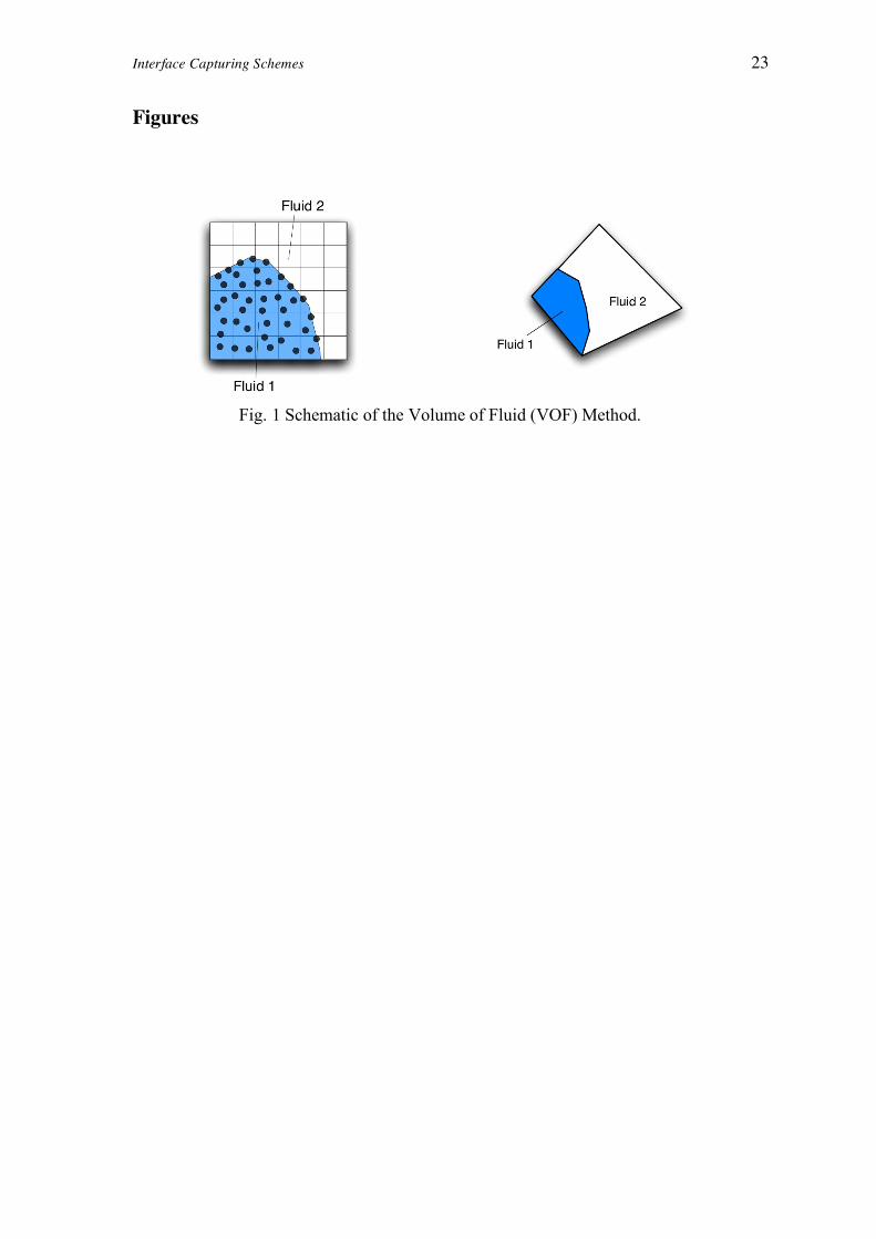
The VOF method, schematically depicted in Fig. 1, is a surface-capturing method for

predicting flows composed of multiple immiscible fluids. The various fluids are

assumed to share a common velocity field and solutions are obtained by solving the

following averaged set of Navier-Stokes equations:


�

! "( )

!t+ # $ "v( ) = 0

! "v( )

!t+ # $ "vv( ) = # $ % &#P + B

(1)

with density and viscosity evaluated using the following relations

fluidsofnumbernwhere

r

r

n

k

)k()k(

n

k

)k()k(

=

=

=

!

!

=

=

1

1

µµ

""

(2)

where r(k) represents the volume fraction of the kth fluid. These r(k) fields are computed

by solving scalar convection equations defined as

( ) fluidsofnumbernn,....,kforrt

r )k()k(

=!=="#+$

$1210v (3)

and constrained by a conservation of volume equation given by

fluidsofnumbernn,....,kforrn

k

)k(===!

=

211

1

(4)

For the case of incompressible fluids the continuity equation can be simplified to

0=!" v (5)

It is this form of the continuity equation (Eq. (5)) that is used in the derivation of the

pressure correction equation in order to avoid numerical difficulties that arise when

large disparities in fluid densities exist.

Interface Capturing Schemes

From the previous section, it is obvious that the success of the VOF method depends

heavily on the interface capturing scheme used in advecting the r field at a control

volume face. The main difficulty associated with the development of such an

advection scheme stems from the need to treat the discrete interface as an averaged

scalar value over a computational cell. This weakness is illustrated, for example, by

considering the advection of a rectangular fluid region over a time interval ∆t with a


courant number of 0.5. The UPWIND scheme gives the solution shown in Fig. 2(a)

while the exact solution is depicted in Fig. 2(b). The smearing of the profile is an

outcome of treating the volume fraction as a standard scalar field rather than a

representation of a fluid-fluid interface. A more appropriate treatment would be to use

an interpolation profile for the r field that lumps the fluid near the interface in the

manner shown in Fig. 2(b). This can be readily done with a downwind interpolation

profile at the highlighted cell face.

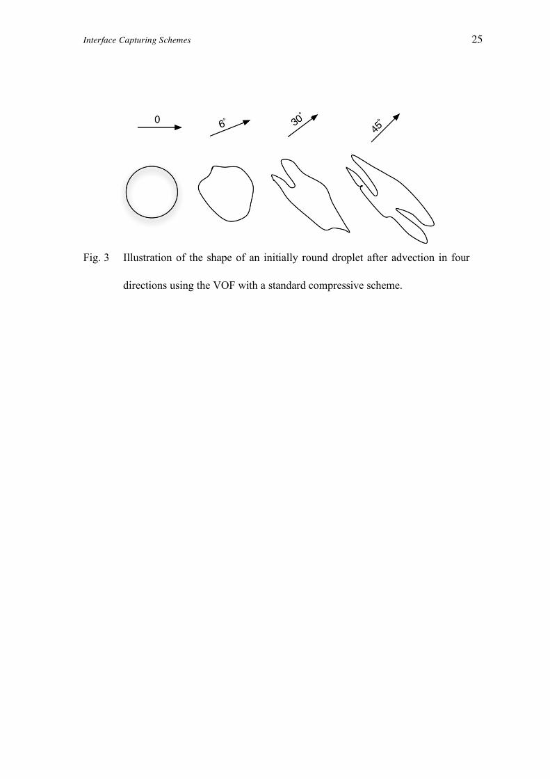
Another difficulty is the well-known false diffusion problem of first order schemes,

which deteriorate in accuracy when the flow is not oriented along a grid line (see Fig.

3). This drawback should preclude using the UPWIND scheme for capturing

interfaces. Moreover, the DOWNWIND scheme being first order accurate, its

performance is also highly dependent on the orientation of the flow relative to the

grid. The effect in this case would be an over-compressed interface with no curvature

(stepping effect). This artificial steepening of the r field was demonstrated by Leonard

[39] through the advection of a one-dimensional semi-elliptic profile that was

transformed into a step profile because of the use of a downwind-like advection

scheme.

Blending Strategy for Interface-Capturing Schemes

One way to address these two shortcomings is through a switching strategy that

depends on the angle between the flow direction and the grid lines [29,40]. The best

approach is to have a continuous switching function whereby the values of a

Compressive and a High-Resolution advection scheme are blended together, with the

blending factor depending on the angle between the flow direction and the grid lines.

The angle can be determined using the grid orientation at the integration face and the

gradient of the r field, whose unit vector represents the direction normal to the


interface (see Fig. 4). This general approach has been followed in the derivation of the

new STACS scheme and is also utilized in the CICSAM [34] and the HRIC [36]

schemes, even though different blending functions are used in these schemes, as will

be described later.

From the above it is clear that an “interface Capturing” scheme based on the

switching strategy should possess the following attributes:

a. It should be based on a combination of Compressive and High-Resolution

schemes.

b. Its blending function should be based on the angle between the interface direction

and the grid orientation, preferably in a continuous fashion.

The Blending Function

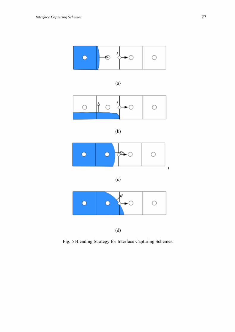
The reasoning followed in defining the blending function is illustrated in Fig. 5. If the

cell has started to be filled with fluid from the upwind side of the interface and the

interface is parallel to the cell face (Fig. 5(a)) then only fluid present at the

downstream cell should be convected through the cell face. In this case a compressive

scheme should be used. However if the interface is perpendicular to the cell face

(Figure 5(b)) then the convected fluid is expected to be of the same composition as

the upwind cell, in this case a HR scheme would be appropriate. When the fluid-fluid

interface is parallel to the cell face but most of the cell is filled with fluid from the

upwind side of the interface (Figure 5(c)), then either scheme could be used. The

above mentioned situations represent extreme cases in which the fluid-fluid interface

is either parallel or perpendicular to the control volume face. In general, the angle

between the interface and cell face is between these two extremes (i.e. the angle θ

usually varies between 0 and 90, Figure 5(d)) and the value of r at the interface should


be obtained by blending the advection schemes of the extreme cases, with the

blending function given as

( ) ( ) ( )[ ]fHRff)eCompressiv(f)(ff fr~fr~r~r~ !!!

"+== 1 (6)

where

�

f ! f( ) is a function that varies between 0 and 1 and r~ is the normalized value

of r defined as

UD

U

rr

rrr~

!

!= (7)

with the subscripts U and D referring to values at the upstream and downstream

locations as shown in Fig. 2.

HRIC Scheme

The High Resolution Interface Capturing scheme (HRIC) of Muzaferija [36,41] is

based on a blending of the Bounded Downwind (BD) and Upwind Differencing

schemes (UD), with the aim of combining the compressive property of the BD

scheme, which can be viewed as a steady-state version of the Hyper-C scheme [39],

with the stability of the UD scheme. The normalized functional relationship of the BD

scheme, whose Normalized Variable Diagram is displayed in Fig. 6, is given by

!"

!#

$

%<

%<

=

otherwiser~r~.

.r~r~

r~

C

C

CC

)BD(f 1501

5002

(8)

The functional relationship of the HRIC scheme is also function of the angle θ

between the normal to the interface (defined by the gradient of the r field) and the

normal to the cell face [41]. For an interface aligned with the cell face (θ=0) the

bounded downwind scheme is used, while for an interface perpendicular to the cell

face the upwind scheme is used. For an interface with θ between these two limits,

�

f ! f( ) is chosen to be

�

cos ! f( ) and the blending formula is given by


( ) ( ) ( )( )fUPWINDff)BD(f)(f cosr~cosr~r~ !!!

"+= 1 (9)

With this formulation (Eq. (9)), the blending of the UPWIND and DOWNWIND

schemes is dynamic and accounts for the local distribution of the r field. Muzaferija

further modifies the value of fr~ to account for the local Courant number (Co) defined

by

�

Cof =v f !S f"t

Vf

(10)

For Courant number below 0.3 the scheme is not modified( ))(ff r~r~.e.i!

= , while for a

courant number above 0.7 the upwind scheme is used. For Co values between 0.3 and

0.7, the interface value computed from Eq. (9) is blended with the upwind scheme to

yield the final r value at the fluid-fluid interface, which in normalized form is written

as

( )3070

70

..

Co.r~r~r~r~

f

)UPWIND(f)(f)(ff!

!!+=

"" (11)

The Normalized Variable Diagrams of the HRIC scheme for Co values in the various

regimes are depicted in Fig. 7. It is clear from the NVD diagram that for courant

number values above 0.7 the HRIC scheme basically reverts to the very diffusive

UPWIND scheme, and even for moderate values of the Courant number, the scheme

would still be very diffusive.

CICSAM Scheme

The CISCAM scheme of Ubbink [34] is also an interface capturing scheme based on

the blending strategy. However rather than choosing the DOWNWIND and UPWIND

schemes as base schemes, it uses, respectively, the HYPER-C scheme [42] and the

ULTIMATE-QUICKEST scheme of Leonard [43], with HYPER-C being utilized

when the cell face is perpendicular to the interface normal vector and the


ULTIMATE-QUICKEST (UQ) employed when the normal vector to the face is

aligned with the normal to the interface. The HYPER-C scheme is a bounded

downwind scheme that is constructed by enforcing the transient CBC criterion onto

the DOWNWIND scheme and is expressed as

!"

!#$

%%&'(

)*+

=,

otherwiser~

r~

Co

r~,min

r~

C

CC

)CHYPER(f

101 (12)

Moreover, the normalized functional relationship of the UQ scheme is given by

�

˜ r f (UQ )= Co ˜ r f (UPWIND ){ } + 1!Co( ) ˜ r f (QUICK ){ }

where

˜ r f (QUICK )=

3

8+

3

4˜ r C

˜ r f (UPWIND )= ˜ r C

(13)

Furthermore, the CICSAM scheme can mathematically be written as

( ) ( )[ ]f)UQ(ff)CHYPER(f)CICSAM(f fr~fr~r~ !! "+="

1 (14)

The blending function

�

f ! f( ) is based on the angle θf between the gradient of the

volume fraction at the interface and the normal to the cell face (see Fig. 4). The

equations for the angle and blending function are computed from

�

! f = arccos"rf #dPF

"rf dPF (15)

and

�

f ! f( ) =mincos 2! f( ) +1

2,1

"

#

$ $

%

&

' ' (16)

For an angle θf=90˚, i.e. when the interface normal is perpendicular to the cell face

normal,

�

f ! f( ) is zero and the UQ scheme is used, and for θf =0, i.e. when the flow

interface is aligned with the face normal, the HYPER-C scheme is used. The NVD of


the CICSAM scheme, depicted in Fig. 8, reveals that with increasing courant number

the scheme becomes more and more diffusive as its NVF function reverts to the

UPWIND scheme.

STACS Scheme

As will be shown in the results section, predictions generated using the above

schemes deteriorate with increasing values of the courant number as these schemes

blend with the upwind scheme and become identical to it at a courant number of 0.7

for HRIC and 1 for CICSAM. The authors of this article have found this behavior to

be a result of the used temporal bounding, originally designed by Leonard [39] for the

explicit QUICKEST scheme. While this is needed for explicit transient schemes, its

use in an implicit method increases numerical diffusion as explained below.

Jasak [44] has shown that numerical diffusion from convection differencing schemes

can be written as

( ) schemeUPWINDthefordUwithr. ffCC !2

1="#"# (17)

while numerical diffusion from temporal discretization is given by

( )( ) ( )

( ) ( )!!"

!!#

$

%=&

=&'&'

eschemEulerlicitexpthefordUCo

schemeEulerimplicitthefordUCo

withr.

ffmaxT

ffmaxT

T

(

(

2

1

2

1

(18)

It is clear that the numerical anti-diffusion (negative diffusion) resulting from the

explicit Euler scheme cancels the numerical diffusion of the upwind scheme at

Courant number of 1. Therefore the use of the upwind scheme as the courant number

approaches 1 is actually desirable with the explicit Euler scheme. On the other hand

the numerical diffusion of the Implicit Euler scheme adds (rather than cancels) to that

resulting from the UPWIND scheme with the total numerical diffusion increasing


with the Courant number and yielding excessively diffusive profiles. This clearly

explains the deterioration in performance experienced by the HRIC and CICSAM

schemes with increasing Courant number.

The deficiencies associated with the above schemes have motivated the development

of a new interface capturing scheme based on the aforementioned strategy but that

overcomes the outlined shortcomings. In the newly suggested Switching Technique

for Advection and Capturing of Surfaces scheme (STACS), the selected compressive

scheme is SUPERBEE [42], a bounded version of the downwind scheme, while the

High-Resolution scheme is STOIC [45]. Moreover, because of the use of an implicit

transient discretization, no transient bounding is applied. Furthermore in order to

minimize the stepping behavior of the highly compressive SUPERBEE scheme, the

blending between the two schemes is performed using equation (6) with

�

f ! f( ) set to

�

cos ! f( )[ ]4

that enables a rapid but smooth switching away from the Compressive

scheme for the case where the normal to the free surface face is not along the grid

direction. The normalized variable diagrams of the SUPERBEE, STOIC and STACS

schemes are displayed in Figs. 9(a), 9(b), and 9(c) respectively.

The normalized variables relationship for the STACS scheme is given by

�

˜ r f ,STACS = ˜ r f ,SUPERBEE cos !( )4

+ ˜ r f ,STOIC 1" cos !( )4

( ) (19)

where SUPERBEE,fr~ and STOIC,fr

~ are obtained from

�

˜ r f ,SUPERBEE =

˜ r C ˜ r C ! 0

1 0 < ˜ r C < 1

˜ r C 1! ˜ r C

"

# $

% $

�

˜ r f ,STOIC =

˜ r C ˜ r C ! 0

1

2+

1

2˜ r C 0 < ˜ r C ! 1

2

3

8+

3

4˜ r C

1

2< ˜ r C ! 5

6

1 5

6< ˜ r C !1

˜ r C 1 < ˜ r C

"

#

$

$ $

%

$

$ $

(20)


This strategy is not limited to the above schemes rather it can be used to devise a

family of free-surface advection schemes by using different combination of

Compressive/HR schemes (e.g. SMART [43], OSHER [46], etc…).

Results and Discussion

This section presents four test cases comparing the performance of the CICSAM,

HRIC, and the new STACS interface capturing schemes in addition to the well-known

UPWIND and SMART schemes over structured and unstructured grid systems.

Results generated are reported in the form of r-contour plots for three values of the

Courant number. In all figures, contours are displayed for 0.05 ≤ r ≤ 0.95 with a step

size Δr=0.06923. All residuals are normalized by their respective local fluxes and at

any time step computations are terminated when the maximum normalized residual

drops below a very small number εs, which is set to 10-6. Moreover, all calculations

are performed assuming that the densities of the fluid and convected shape are equal

and surface tension effects are negligible. The exact solutions for the problems

considered are presented in Fig. 10.

Advection of Hollow Shapes in an Oblique Velocity Field

Three different hollow shapes [47,37] are convected in an oblique velocity field

defined by v[2,1]. The computational domain is a square of side 1m, subdivided into

200x200 (40,000) square control volumes for structured grid computations and 47,240

triangular elements for unstructured grid calculations. The following three shapes,

depicted in Figs. 10(a), 10(b), and 10(c), are considered:

1. A hollow square (Fig. 10(a)) aligned with the co-ordinate axes of an outer side

length 0.2m and inner side length 0.1m, which for the structured mesh used are

subdivided into 40 and 20 cells respectively.


2. A hollow square rotated through an angle of 26.57˚ with respect to the x-axis (Fig.

10(b)) of dimensions similar to those of the above hollow square.

3. A hollow circle (Fig. 10(c)) with an outer diameter of length 0.2m and inner

diameter of 0.1 m spanning 40 and 20 structured cells respectively.

All shapes are initially centered at (0.2, 0.2) m with their exact positions centered at

(0.8, 0.5) m after 0.3 s, as displayed in Figs. 10(a)-10(c). Computations, using the

second order Crank-Nicholson scheme, are performed for three different time steps

∆t= 0.0004167, 0.0008333, and 0.0012498 s yielding, over the structured grids, a

Courant number of value 0.25, 0.5, and 0.75 respectively. Since it is hard to control

the Courant number over the unstructured grid, these values are denoted by low,

medium, and high on the presented results. The Courant number is defined as

�

Co =vP !S f( ),0 "t

VP~ f P( )

# (21)

which for Cartesian grid recovers its standard multi-dimensional form given by

y

tv

x

tuCo

!

!+

!

!= (22)

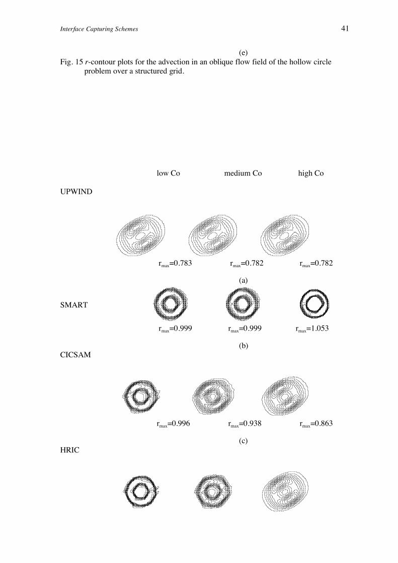
Contour plot results of the r fields for the various shapes and schemes at different Co

values after the lapse of 0.3 s are presented in Figs. 11-16. As depicted, the trend is

the same for all shapes. The UPWIND scheme profiles (Figs. 11(a)-16(a)) are highly

diffusive at all Co considered. The Smart scheme produces results that are better than

those obtained with the upwind scheme however it does not resolve sharply the

interfaces (Figs. 11(b)-16(b)). The Co seems to have little effect on the convected

shapes predicted by both schemes with the maximum value of r slightly varying. On

the other hand, results generated by the CICSAM (Figs. 11(c)-16(c)) and HRIC (Figs.

11(d)-16(d)) schemes show high dependence on Co with the predicted shapes


becoming increasingly diffusive with increasing values of Co. As expected, the

maximum predicted value of r decreases as Co increases since the schemes approach

the UPWIND scheme. The HRIC and CICSAM schemes revert to the UPWIND

scheme at Co≥0.7 and 1, respectively. This explains the analogous shapes obtained by

the HRIC and UPWIND schemes at Co=0.75. The best profiles are the ones obtained

by the newly developed STACS scheme (Figs. 11(e)-16(e)), which are almost

independent of Co with a maximum r value of 1 and preserving the sharpness of the

interfaces. The better performance of STACS in comparison with other schemes is

due to the reasons explained in the previous section.

By comparing contours obtained over structured (Figs. 11, 13, and 15) and

unstructured meshes (Figs. 12, 14, and 16), it is clear that results follow similar trends

with the quality of those obtained on structured rectangular grids being slightly better.

The small wiggles that are mildly polluting some of the unstructured grid results are

due to larger variations in the blending angle θ as compared to the structured grid

case. This is in addition to a higher Co value due to the larger number of triangular

elements. Nevertheless the performance of STACS is by far more superior to all other

schemes.

Advection of a Slotted Circle in a Rotational Flow Field

The solid-body rotation of an object poses a test problem with a trivial exact solution

[47,38,48]. However it is a tough problem with regard to advection schemes. The test

in question involves the rotation of a slotted circle around an external point. The

computational domain, schematically depicted along with the exact solution in Fig.

10(d), is a square of dimensions [4, 4] m discretized into 200x200 (40,000) square

control volumes for structured grid computations giving a step size of Δx=Δy=5x10-3


and 65,536 triangular elements for unstructured grid calculations. The circle of

diameter 1 m (occupying 50 structured cells) has its centre at (2,2.65) m and is cut by

a slot of width 0.12 m (occupying 6 structured cells). The rotation of the slotted circle

is driven by a vortex flow centered at the middle of the domain (2,2) of angular

velocity ω=0.5 rad/s. The time required by the slotted circle to complete a revolution

is 2π/ ω s. With the geometry considered, the Courant number varies from a minimum

(equals to 0.15*ω*Δt/Δx) at point (2, 2.15) to a maximum (equals to 1.15*ω*Δt/Δx) at

(2, 2.65). The problem is solved for three different local Courant number values such

that the total period required for a revolution is subdivided into 1262, 841, and 421

time steps, respectively.

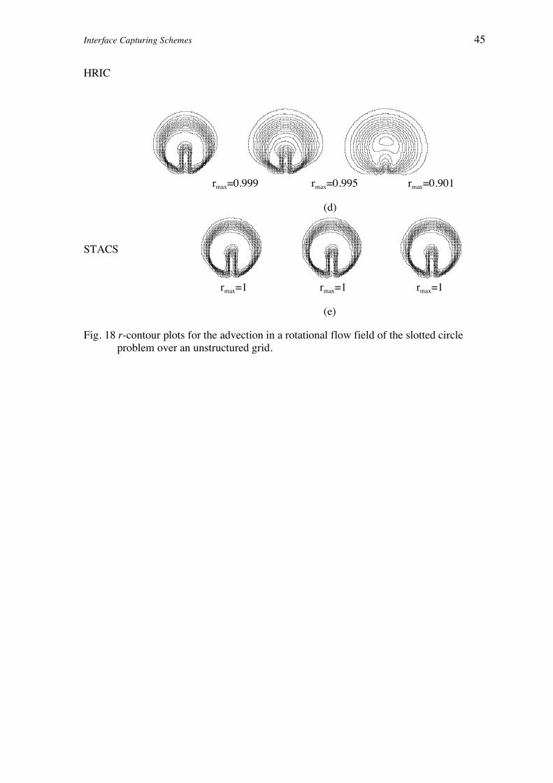
As for the previous tests, predictions generated by the various schemes over

structured and unstructured grids are presented in the form of contour plots for the r

field in Figs. 17 and 18, respectively. The trend of results generated by the UPWIND

(Figs. 17(a) and 18(a)), SMART (Fig. 17(b) and 18(b)), and STACS (Fig. 17(e) and

18(e)) is the same as for the previous test cases. Profiles generated by CICSAM (Fig.

17(c) and 18(c)) and HRIC (Fig. 17(d) and 18(d)) may look different than the ones

generated earlier but are essentially similar as will be clarified. For these two

schemes, contours are more diffusive on the upper side. This is due to the variation in

the Courant number, which is higher on the upper side than on the lower side. Unlike

the previous test cases for which the Co was constant, in this problem it increases with

distance from the center of rotation. As the local value of Co increases, the

contribution of the upwind value to the scheme increases resulting in the displayed

profiles. Other schemes do not seem to be affected by the Courant number as their

functional relationships are not affected by its value. Again structured grid results

(Fig. 17) are more accurate than unstructured grid predictions (Fig. 18) due to a higher


Courant number resulting from the larger number of triangular elements used. The

best performance however remains for STACS, which is capable of resolving all

interfaces accurately and at all Co considered.

Closing Remarks

A general methodology for constructing interface capturing schemes based on a

switching strategy was presented. The method was used to develop a new interface

capturing scheme denoted by STACS. The accuracy of the newly developed scheme

on structured and unstructured grid networks was compared against the UPWIND,

SMART, CICSAM, and HRIC schemes by solving several pure advection problems

and was shown to be by far more accurate preserving sharpness of interfaces. Unlike

the HRIC and CICSAM schemes, STACS’s performance was shown to be

independent, for all cases considered, of the Courant number value.


Figure Captions

Fig. 1 Schematic of the Volume of Fluid (VOF) Method.

Fig. 2 Advection of a fluid block at a courant number of value 0.5 using (a) the

upwind scheme and (b) the exact solution.

Fig. 3 Final shape of an initially round droplet after advection in four directions

using the VOF with a standard compressive scheme.

Fig. 4 Angle between interface and cell face.

Fig. 5 Blending Strategy for Interface Capturing Schemes.

Fig. 6 The Normalized Variable Diagram (NVD) of the Bounded Downwind

Scheme.

Fig. 7 The Normalized Variable Diagram (NVD) of the HRIC scheme.

Fig. 8 The Normalized Variable Diagram (NVD) of the CICSAM scheme.

Fig. 9 The Normalized Variable Diagrams (NVD) of the (a) SUPERBEE, (b)

STOIC, and (c) STACS scheme.

Fig. 10 Schematics of the advected (a) hollow square, (b) rotated hollow square, (c)

hollow circle, and (d) slotted circle problems.

Fig. 11 r-contour plots for the advection in an oblique flow field of the hollow

square problem over a structured grid.


Fig. 12 r-contour plots for the advection in an oblique flow field of the hollow

square problem over an unstructured grid.

Fig. 13 r-contour plots for the advection in an oblique flow field of the rotated

hollow square problem over a structured grid.

Fig. 14 r-contour plots for the advection in an oblique flow field of the rotated

hollow square problem over an unstructured grid.

Fig. 15 r-contour plots for the advection in an oblique flow field of the hollow circle

problem over a structured grid.

Fig. 16 r-contour plots for the advection in an oblique flow field of the hollow circle

problem over an unstructured grid.

Fig. 17 r-contour plots for the advection in a rotational flow field of the slotted circle

problem over a structured grid.

Fig. 18 r-contour plots for the advection in a rotational flow field of the slotted circle



Figures

Fig. 1 Schematic of the Volume of Fluid (VOF) Method.


(a) (b)

Fig. 2 Advection of a fluid block at a courant number of value 0.5 using (a) the

upwind scheme and (b) the exact solution.


Fig. 3 Illustration of the shape of an initially round droplet after advection in four

directions using the VOF with a standard compressive scheme.


Fig. 4 Angle between interface and cell face.


(a)

(b)

(c)

(d)

Fig. 5 Blending Strategy for Interface Capturing Schemes.


Fig. 6 The Normalized Variable Diagram (NVD) of the Bounded Downwind Scheme.


Fig. 7 The Normalized Variable Diagram (NVD)of the HRIC scheme.


Fig. 8 The Normalized Variable Diagram (NVD)of the CICSAM scheme.


(a) (b)

(c)

Fig. 9 The Normalized Variable Diagrams (NVD)of the (a) SUPERBEE, (b) STOIC,

and (c) STACS scheme.


(a) (b)


(c) (d)

Fig. 10 Schematics of the advected (a) hollow square, (b) rotated hollow square, (c) hollow circle, and (d) slotted circle problems.


low Co medium Co high Co UPWIND

rmax=0.545 rmax=0.545 rmax=0.546

(a) SMART

rmax=0.993 rmax=0.991 rmax=0.990

(b) CICSAM

rmax=0.994 rmax=0.971 rmax=0.938

(c) HRIC

rmax=0.995 rmax=0.780 rmax=0.546

(d)


STACS

rmax=1 rmax=1 rmax=1

(e) Fig. 11 r-contour plots for the advection in an oblique flow field of the hollow square

problem over a structured grid. low Co medium Co high Co UPWIND

rmax=0.765 rmax=0.765 rmax=0.765

(a)

SMART

rmax=0.997 rmax=0.997 rmax=1.044

(b) CICSAM

rmax=0.990 rmax=0.946 rmax=0.852

(c)


HRIC

rmax=0.996 rmax=0.973 rmax=0.810

(d)

STACS


(e) Fig. 12 r-contour plots for the advection in an oblique flow field of the hollow square




rmax=0.550 rmax=0.550 rmax=0.550

(a) SMART

rmax=0.998 rmax=0.997 rmax=0.997

(b) CICSAM

rmax=0.998 rmax=0.984 rmax=0.940

(c) HRIC

rmax=1.003 rmax=0.805 rmax=0.550

(d)


STACS


(e) Fig. 13 r-contour plots for the advection in an oblique flow field of the rotated hollow

square problem over a structured grid. low Co medium Co high Co UPWIND

rmax=0.874 rmax=0.874 rmax=0.874

(a) SMART

rmax=1 rmax=1 rmax=1.009

(b) CICSAM


rmax=0.999 rmax=0.958 rmax=0.918

(c) HRIC

rmax=0.999 rmax=0.981 rmax=0.895

(d) STACS


(e) Fig. 14 r-contour plots for the advection in an oblique flow field of the rotated hollow

square problem over an unstructured grid.



rmax=0.512 rmax=0.512 rmax=0.513

(a) SMART

rmax=0.994 rmax=0.994 rmax=1.009

(b) CICSAM

rmax=0.996 rmax=0.971 rmax=0.929

(c) HRIC

rmax=0.994 rmax=0.750 rmax=0.513

(d) STACS



(e) Fig. 15 r-contour plots for the advection in an oblique flow field of the hollow circle


rmax=0.783 rmax=0.782 rmax=0.782

(a)

SMART

rmax=0.999 rmax=0.999 rmax=1.053

(b) CICSAM

rmax=0.996 rmax=0.938 rmax=0.863

(c) HRIC


rmax=0.998 rmax=0.968 rmax=0.827

(d)

STACS


(e) Fig. 16 r-contour plots for the advection in an oblique flow field of the hollow circle




rmax=0.778 rmax=0.778 rmax=0.778

(a)

SMART


(b) CICSAM

rmax=1 rmax=1 rmax=0.971

(c) HRIC

rmax=1.004 rmax=1.005 rmax=0.878

(d)

STACS



(e) Fig. 17 r-contour plots for the advection in a rotational flow field of the slotted circle


rmax=0.893 rmax=0.893 rmax=0.893

(a)

SMART

rmax=0.999 rmax=0.999 rmax=1

(b) CICSAM

rmax=0.990 rmax=0.974 rmax=0.926

(c)


HRIC

rmax=0.999 rmax=0.995 rmax=0.901

(d)

STACS


(e) Fig. 18 r-contour plots for the advection in a rotational flow field of the slotted circle



References

1 Darwish, M. and Moukalled, F.,” An exact r-Factor TVD Formulation for

Unstructured Grids,” IASTED International Conference on Applied Simulation

and Modeling, Crete, Greece, June 25-28, 2002.

2 Darwish, M. and Moukalled, F.,” TVD Schemes for Unstructured Grids,”

International Journal of Heat and Mass Transfer, vol. 46, no. 4, pp. 599-611,

2003.

3 Darwish, M. and Moukalled, F.,“ B-Express: A new Bounded Extrema

Preserving Algorithm Strategy for Convective Schemes”, Numerical Heat

Transfer, Part B: Fundamentals, vol. 37, no. 2, pp 227-246, 2000.

4 Darwish, M. and Moukalled, F.," An Efficient Very High-Resolution Scheme

Based on an Adaptive-Scheme Strategy”, Numerical Heat Transfer, Part B, vol.

34, pp. 191-213, 1998.

5 Darwish, M. and Moukalled, F., “A New Route for Building Bounded Skew-

Upwind Schemes”, Computer Methods in Applied Mechanics and Engineering,

vol. 129, pp. 221-233, 1996.

6 Moukalled, F. and Darwish, M.,”A High-Resolution Pressure-Based Algorithm

for Fluid Flow at All Speeds”, Journal of Computational Physics, vol. 168, no.1,

pp. 101-133, 2001.

7 Moukalled, F. and Darwish, M.,“A Unified Formulation of the Segregated Class

of Algorithms for Fluid Flow at All Speeds,” Numerical Heat Transfer, Part B:

Fundamentals, vol. 37, no. 1, pp 103-139, 2000.


8 Darwish, M., Moukalled, F., and Sekar, B.“ A Unified Formulation of the

Segregated Class of Algorithms for Multi-Fluid Flow at All Speeds,” 36th

AIAA/ASME/SAE/ASEE Joint Propulsion Conference, Huntsville, Alabama,

16-19 July, 2000.

9 Darwish, M., Moukalled, F., and Sekar, B.,“ A Unified Formulation for the

Segregated Class of Algorithms for Multi-Fluid Algorithm at All Speeds,”

Numerical Heat Transfer, Part B: Fundamentals, vol.40, no. 2, pp. 99-137, 2001

10 Shyy, W. and Chen, M.H., ”Pressure-Based Multigrid Algorithm for Flow at All

Speeds,” AIAA Journal, vol. 30, no. 11, pp. 2660-2669, 1992.

11 Brandt, A.,”Multi-Level Adaptive Solutions to Boundary-Value Problems,”

Math. Comp., vol. 31, pp. 333-390, 1977.

12 Rhie, C.M.,”A Pressure Based Navier-Stokes Solver Using the Multigrid

Method,” AIAA paper 86-0207, 1986.

13 Shyy, W. and Braaten, M.E.,” Adaptive Grid Computation for Inviscid

Compressible Flows Using a Pressure Correction Method,” AIAA Paper 88-

3566-CP, 1988.

14 Darwish, M., Moukalled, F., and Sekar, B.,” A Robust Multi-Grid Algorithm for

Multifluid Flow at All Speeds,” International Journal for Numerical Methods in

Fluids, vol. 41, pp. 1221-1251, 2003.

15 Ha, J., Cleary, P.W., Alguine, V., and Nguyen, T., “Simulation of die filling in

gravity die casting using SPH and MAGMA soft”, Proceedings of the Second

International Conference on CFD in the Minerals and Process Industries

Melbourne, 1999.


16 Cleary, P.W. and Ha, J., “Three-dimensional modeling of high pressure die

casting,” Journal of Cast Metals Research, vol.12, pp. 357-365, 2000.

17 Nichols, B.D., Hirt, C.W., and Hotchkiss, R.S.,” SOLA-VOF: a solution

algorithm for transient fluid flow with multiple free boundaries,” Technical

Report LA-8355, Los Alamos Scientific Laboratory, 1980.

18 Nichols, B.D. and Hirt, C.W.," Methods for Calculating Multi-Dimensional,

Transient Free-Surface Flows Past Bodies," Proceedings of First International

Conference of Numerical Ship Hydrodynamics, Gaithersburg, ML, Oct. 20-23,

1975.

19 Hirt, C.W. and Nichols, B.D., "Volume of Fluid (VOF) Method for the

Dynamics of Free Boundaries," J. Comp. Physics, vol. 39, pp. 201, 1981.

20 Leonard, B.P. and Mokhtari, S.,” Beyond First–Order Upwinding: The Ultra–

Sharp Alternative for Non–Oscillatory Steady–State Simulation of Convection,”

International Journal for Numerical Methods in Engineering, vol. 30, pp.729-

766, 1990.

21 Youngs, D.L.,” An interface tracking method for a 3D Eulerian hydrodynamics

code”, Technical Report 44/92/35, Atomic Weapons Research Establishment,

1984.

22 Puckett, E.G.,” A volume of fluid interface tracking algorithm with applications

to computing shock wave rarefraction,” Proceedings of the Fourth International

Symposium on Computational Fluid Dynamics, University of California at

Davis, CA, 9–12 September, pp. 933–938, 1991.


23 Unverdi, S.O. and Tryggvason, G.,“ A front tracking method for viscous,

incompressible multi-fluid flow”, Journal of Computational Physics, vol. 100,

pp. 25-37, 1992.

24 Noh, W.F. and Woodward, P., “SLIC (Simple Line Interface Calculations)”,

Lecture Notes in Physics, Vol. 59, pp. 330-340, 1976.

25 Rudman, M.,“ Volume tracking methods for interfacial flow calculations”,

International Journal for Numerical Methods in Fluids, vol. 24, pp. 671-691,

1997.

26 Renardy, Y. and Renardy M., “PROST: Parabolic Reconstruction of Surface

Tension for the volume-of-fluid Method”, Journal of Computational Physics,

vol.183, No. 2, pp. 400-421, 2002.

27 Harvie D.J.E, Fletcher D.F., “A new Volume of fluid advection algorithm: the

defined donating region scheme”, Int. J. Num. Methods Fluids, vol. 38, p. 151-

172, 2001

28 Harlow, F.H. and Amsden, A.A., Fluid dynamics. Los Alamos National

Laboratory report LA-4700, 1971.

29 Lafaurie, B., Nardone, C., Scardovelli, R., Zaleski, S., and Zanetti, G.,”

Modelling merging and fragmentation in multiphase flows with SURFER,”

Journal of Computational Physics, vol. 113, pp. 134-147, 1994.

30 Maronnier, V., Picasso, M., and Rappaz, J.,” Numerical Simulation of Free

Surface Flows,” Journal of Computational Physics, vol. 155, pp. 439-455, 1999.

31 Kothe, D.B., Williams, M.W., Lam, K.L., Korzekwa, D.R., Tubesing, P.K., and

Puckett, E.G.,” A Second-Order accurate , Linearity preserving volume tracking


Algorithm for Free-Surface flows on 3-D unstructured meshes,” Proceedings of

the 3rd ASME, JSME Joint Fluids Engineering Conference, San Francisco,

California, USA, July 18-22, 1999.

32 Brackbill, J.U., Kothe, D.B., and Zemach, C.,“ A Continuum Method for

Modelling Surface Tension,” Journal of Computational Physics, vol. 100, pp.

335-354, 1992.

33 Kothe, D.B., and Mjolsness, R.C.,” RIPPLE: A new model for incompressible

flows with free Surfaces,” AIAA Journal , vol 30, no. 11, pp 2694-2700, 1992.

34 Ubbink, O. and Issa, R.,“ A Method for Capturing Sharp Fluid Interfaces on

Arbitrary Meshes”, Journal of Computational Physics, vol. 153, pp. 26-50,

1999.

35 Moukalled F., Darwish M.S.," A New Bounded-Skew Central Difference

Scheme- part I: Formulation & Testing,” Numerical Heat Transfer, Part B:

Fundamentals, vol. 31, pp. 91-110, 1996.

36 Muzaferija S., and Peric M.,” Computation of free-surface flows using

interface-tracking and interface-capturing methods,” in Mahrenholtz O,

Markiewicz M. (eds.), Nonlinear Water Wave Interaction, Computational

Mechanics Publications, Southampton, 1998.

37 Rider, W.J. and Kothe, D.B.,“ Stretching and Tearing Interface Tracking

Methods,” AIAA Paper 95-1717, Presented at the 12th AIAA CFD Conference,

San Diego, June 19-22, LANL Report LA-UR-95-1145, 1995.

38 Rider, W.J. and Kothe, D.B.,” Reconstructing Volume Tracking,” Journal of

Computational Physics, vol. 141, pp. 112-152, 1998.


39 Leonard B.P., ”The ULTIMATE Conservative Difference Scheme Applied to

Unsteady One-Dimensional Advection,” Computer Methods in Applied

Mechanics and Engineering, vol. 88, pp. 17-74, 1991.

40 Ramshaw, J.D. and Trapp, J.A.,”Numerical Technique For Low Speed

Homogeneous Two Phase Flow with a Sharp Interface”, J. Computational

Physics, vol. 21, pp. 438, 1976.

41 Muzaferija, S., Peric, M., Sames, P., and Schellin, P.,“ A Two-Fluid Navier-

Stokes solver to Simulate Water Entry,” Proceedings of the Twenty-Second

Symposium on Naval Hydrodynamics, pp.638-649, 1998.

42 Leonard, B.P. and Niknafs, H.S.,“ Sharp monotonic resolution of discontinuities

without clipping of narrow extrema,” Computers and Fluids, vol. 19, no. 1, pp.

141-154, 1991.

43 Leonard, B.P.,“ Stable and accurate convective modeling procedure based on

quadratic upstream interpolation,“ Computer Methods in Applied Mechanics

and Engineering, pp. 59-98, 1990.

44 Jasak, H.,“ Error Analysis and Estimation for the Finite Volume Method With

Applications to Fluid Flows,” Ph.D Thesis, Department of Mechanical

Engineering, Imperial College of Science, Technology and Medecine, June

1996.

45 Darwish, M.,“ A New High-Resolution Scheme Based on the Normalized

Variable Formulation,” Numerical Heat Transfer, part B, vol. 24, pp. 353-373,

1993.


46 Osher, S. and Chakravarthy, S.,” Upwind schemes and boundary conditions

with applications to Euler equations in general geometries,” Journal of

Computational Physics, vol. 50, pp. 447–481, 1983.

47 Rudman, M.,” Volume-Tracking Methods for Interfacial Flow Calculations, ”

International Journal for Numerical Methods in Fluids, vol. 24, pp. 671-691,

1997.

48 Zalesak, S.T.,” Fully Multi-Dimensional Flux Corrected Transport Algorithms

for Fluid Flow,” Journal of Computational Physics, vol. 31, pp. 335-362, 1979.

Documents

Convective Schemes for Capturing Interfaces of …Convective Schemes for Capturing Interfaces of Free-Surface Flows on Unstructured Grids M. Darwish and F. Moukalled American University