Embed Size (px)
Citation preview

Controlling the mobility in nanostructured
environments by stimuli-responsive polymers
Dissertation
zur Erlangung des Grades
"Doktor der Naturwissenschaften"
am Fachbereich Chemie
der Johannes Gutenberg-Universität Mainz
Jing Xie
geboren am 29.04.1988
in Guangan (China)
Mainz – 2015

2

3
Dekan:
1. Berichterstatter:
2. Berichterstatter:
Tag der mündlichen Prüfung: 11.02.2016

4
Die vorliegende Arbeit wurde im Zeitraum von Oktober 2012
bis Februar 2016 am Max‐Planck‐Institut für Polymerforschung,
unter der Betreuung von ... und ... angefertigt.

5
Table of Contents
Abstract ......................................................................................................................... 9
Zusammenfassung ....................................................................................................... 10
CHAPTER 1 Introduction ........................................................................................... 11
1.1 Diffusion ................................................................................................................ 11
1.1.1. Fick’s laws ..................................................................................................... 12
1.1.1.1 Fick’s first law ......................................................................................... 12
1.1.1.2 Fick’s second Law ................................................................................... 13
1.1.2 Einstein-Smoluchowski relation ..................................................................... 15
1.1.3 Applications .................................................................................................... 18
1.2. Stimuli-responsive polymers ................................................................................ 18
1.2.1 Thermo-responsive polymers ......................................................................... 19
1.2.1.1 Poly(N-isopropylacrylamide) .................................................................. 19
1.2.1.2 The lower critical solution temperature ................................................... 20
1.2.1.3 Applications ............................................................................................. 22
1.2.2 pH-responsive polymers ................................................................................. 23
1.2.2.1 Poly(2-diethylaminoethyl methacrylate) ................................................. 24
1.2.2.2 Applications ............................................................................................. 24
1.2.3 Other stimuli-responsive polymers ................................................................. 25
1.2.4 Morphology of stimuli-responsive polymers ................................................. 25
1.2.4.1 Films ........................................................................................................ 26
1.2.4.2 Particles .................................................................................................... 28
1.2.4.3 Other morphologies ................................................................................. 30
1.3 Motivation ............................................................................................................. 31
CHAPTER 2 Methods ................................................................................................. 33
2.1 Principle of fluorescence correlation spectroscopy (FCS) .................................... 33
2.2 FCS experimental setup ......................................................................................... 37
2.3 Scanning electron microscopy ............................................................................... 38
2.4 pH meter ................................................................................................................ 39

6
2.4.1 pH adjustment.................................................................................................. 39
2.5 Gel permeation chromatography ............................................................................ 39
2.6. Materials ................................................................................................................ 39
2.6.1 Fluorescent dyes .............................................................................................. 39
2.6.1.1 Alexa series............................................................................................... 41
2.6.1.2 Bodipy ...................................................................................................... 42
2.6.1.3 Quantum dots ............................................................................................ 43
2.6.2 Silica inverse opals .......................................................................................... 44
2.6.2.1 Silica and PS nanoparticles....................................................................... 45
2.6.2.2 Preparation ................................................................................................ 45
2.6.3 PS/PDEA hairy nanoparticles and PDEA single chains ................................. 48
2.6.4 Cells for FCS measurement ............................................................................. 48
2.7 Atom transfer radical polymerization (ATRP)....................................................... 49
2.7.1 “Grafting from” ............................................................................................... 53
2.7.2 “Grafting to” .................................................................................................... 54
CHAPTER 3 Temperature controlled diffusion in PNIPAM modified silica inverse
opals ................................................................................................................................. 55
3.1 Introduction and motivation ................................................................................... 55
3.2 Atom transfer radical polymerization on silica inverse opals ................................ 58
3.2.1 Preparation of the silica inverse opals ............................................................. 58
3.2.2 ATRP on silica inverse opals .......................................................................... 59
3.2.2.1 Materials ................................................................................................... 59
3.2.2.2 Initiator immobilization ............................................................................ 60
3.2.2.3 Surface-initiated polymerizations ............................................................. 60
3.3 Dyes and solvents for FCS measurement ............................................................... 63
3.4 Alexa 647 and QD 525 diffusion in PNIPAM grafted silica inverse opals ........... 63
3.5 Tuning (controlling) the penetrant diffusion .......................................................... 67
3.6 Conclusion .............................................................................................................. 69
CHAPTER 4 pH controlled diffusion of hairy nanoparticles .......................................... 71
4.1 Introduction and motivation ................................................................................... 71

7
4.2 Preparation of Bodipy labeled PS/PDEA hairy nanoparticle and PDEA single
chain ................................................................................................................... 74
4.3 Monitoring the pH-responsive behavior at high concentration ............................. 76
4.4 Monitoring the pH-responsive behavior at individual particle level ..................... 79
4.5 Comparison of the pH-responsiveness of the hairy nanoparticles and single chains
............................................................................................................................ 83
4.6 Controlling the mobility of the pH-responsive particles in nanoporous
environment ....................................................................................................... 85
4.7 Conclusion ............................................................................................................. 89
CHAPTER 5 Summary and conclusion ...................................................................... 91
Acknowledgement ....................................................................................................... 93
List of symbols ............................................................................................................ 95
List of abbreviations .................................................................................................... 97
References ................................................................................................................... 99
Curriculum Vitae ....................................................................................................... 109

8

9
Abstract
Understanding and controlling the diffusion of small molecules, macromolecules
and nanoparticles in solution and complex, nanostructured environments is of paramount
fundamental and technological importance. Often, diffusion is the dominant mechanism for
the transport of such species in e.g. solid nanoporous structures, polymer solutions and gels,
or in living cells. Thus, it is relevant for many processes and applications including drug
delivery, cell nutrition, porous chromatography, polymer synthesis and separation, treatment
of waste water, oil recovery, etc. For all of those applications, one prerequisite is that the
mobility of the species needs to be controllable. To control the mobility of the species, the
size of the species itself or the size and/or density of the nanopores of surrounding
environment can be changed. Stimuli-responsive polymers are ideal candidate materials to
construct both systems, as they are capable of conformational changes when they are
exposed to external stimuli. In addition, they can form versatile configurations such as
mixed polymer brushes, micelles, vesicles, layer-by-layer films, and so on, which provides a
feasible way to construct the responsive species or the responsive environment for mobility
control.
For observation of species’ mobility, fluorescence correlation spectroscopy (FCS)
technique is a well-developed technique. The fluorescent intensity fluctuations caused by
the diffusion of the species through a very small confocal detection volume are recorded and
the change process can be traced. Because of its extremely small detection volume (V< 10-15
L), high sensitivity is reached and even single molecule can be traced in the solution.
Nowadays FCS has been developed as a powerful technique for studying the dynamics of
fluorescent species such as small molecules, macromolecules, or nanoparticles in various
environments in polymer and colloid science.
In this thesis, the species’ mobility has been controlled by combining stimuli-
responsive polymers. For the stimuli-responsive polymers, I choose a typical thermo-
responsive polymer and a pH-responsive polymer, as they are the most classic and widely
used polymers in material science and biology. FCS is used to monitor the mobility of the
species in solution and also in porous media.
In the first part of this thesis, the species mobility has been controlled by changing
the pore size of the surrounding medium. Poly(N-isopropylacrylamide) (PNIPAM) is
grafted onto the well-defined, highly ordered porous network-silica inverse opal. When
temperature increases above the lower critical solution temperature of PNIPAM, PNIPAM
chains collapse accordingly, resulting in an increase of the mobility of the penetrant in the
system, and vice versa.
In the second part of this thesis, the mobility of the nanoparticles has been controlled
by changing the size of the nanoparticle itself. I prepare pH-responsive nanoparticles, which
are composed of pH-insensitive polystyrene cores and pH-responsive poly (2-
diethylaminoethyl methacrylate) (PDEA) hairs. When the pH increases, the PDEA hairs
collapse and the size of the hairy nanoparticle will decrease, which results in faster mobility
of the nanoparticles in the solution. The effect is particularly evident when the nanoparticles
are dispersed in a nanostructured environment.

10
Zusammenfassung
Verständnis und Kontrolle der Diffusion von kleinen Molekülen, Makromolekülen
und Nanopartikeln in Lösung und nanostrukturierter komplexer Umgebung sind von
fundamentaler und technologischer Relevanz. Die Diffusion ist der dominierende
Transportmechanismus solcher Teilchen (z. B. in festen nanoporösen Strukturen,
Polymerlösungen, Gelen oder in lebenden Zellen). Die Diffusion ist daher für viele Prozesse
und Anwendungen wie Wirkstofffreisetzung, Zellernährung, Chromatographie,
Polymersynthesen, Aufbereitung von Abwasser oder Rückgewinnung von Öl relevant.
Durch die Kontrolle der Größe der Teilchen, der Dichte oder Größe der nanoporösen
Umgebung ist es möglich, die Bewegung der zu untersuchenden Teilchen zu kontrollieren.
Ideale Materialien zur Herstellung dieser Systeme sind stimuliresponsive Polymere. Sie
reagieren auf spezifische Anregungen und können abhängig von externen Reizen ihre
Konformation ändern. Außerdem können sie verschiedenste Konfigurationen annehmen,
wie z. B. Bürstenpolymere, Mizellen, Vesikel, geschichtete Filme, usw. Durch externe
Reize ist es möglich, die Mobilität zu kontrollieren.
Zur Beobachtung der Teilchenbewegung eignet sich die
Fluoreszentkorrelationsspektroskopie (FCS – engl. fluorescence correlation spectroscopy).
Dabei diffundieren die fluoreszierenden Teilchen durch ein sehr kleines konfokales
Detektionsvolumen. Die Intensitätsfluktuation der Fluoreszenz wird aufgenommen und
ausgewertet. Durch das sehr geringe Detektionsvolumen (V < 10-15 L) und die hohe
Sensitivität der Methode, können sogar einzelne Moleküle in der Lösung detektiert werden.
Heutzutage ist FCS eine häufig genutzte und sehr gute Methode zur Untersuchung der
Dynamik von fluoreszierenden Teilchen wie kleinen Molekülen, Makromolekülen oder
Nanopartikel in verschiedensten Bereichen der Polymer- und Kolloidwissenschaft.
In der vorliegenden Arbeit wird die Mobilität der Teilchen durch die Kombination
von stimuliresponsiven Polymeren kontrolliert. Hierfür werden auf Temperatur reagierende
Polymere mit pH-abhängigen Polymeren kombiniert, da diese zu den klassischen und häufig
verwendeten Polymermaterialien im Bereich der Biologie zählen. Zur Beobachtung der
Mobilität dieser Teilchen in Lösungen als auch in porösem Material wird FCS verwendet.
Im ersten Teil der Doktorarbeit wird die Teilchenbewegung durch die Veränderung
der Porengröße des umgebenden Mediums kontrolliert. Poly(N-Isopropylacrylamid)
(PNIPAM) wird dafür auf einen inversen Opal mit hoch geordnetem porösen Silicanetzwerk
aufgepfropft. Aufgrund von Temperaturerhöhung über die untere kritische
Lösungstemperatur (LCST – engl. lower critical solution temperature) von PNIPAM,
kollabiert die Polymerkette und verursacht eine Erhöhung der Teilchenbewegung im
System, und umgekehrt.
Im zweiten Teil der Doktorarbeit wird die Mobilität von Nanopartikel durch
Veränderung der Partikel selbst kontrolliert. Nanopartikel aus pH-stabilem Polystyrol-Kern
und pH-abhängigen Polymerbürsten aus Poly(2-Diethylaminoethylmethacrylat) (PDEA)
wurden dafür hergestellt. Wird der pH-Wert erhöht, kollabieren die PDEA-Bürsten und die
Größe des Partikels verringert sich, was zu schnellerer Teilchenbewegung in der Lösung
führt. Dieser Effekt zeigt sich besonders deutlich, wenn die Nanopartikel in
nanostrukturierter Umgebung verteilt sind.

11
CHAPTER 1
Introduction
1.1 Diffusion
Diffusion is the spontaneous transport of mass in gases, liquids and solids from a
high concentration to low concentration, until equilibrium is finally reached in the whole
system. Diffusion is an irreversible process which leads to an increase in entropy and
can only be reversed by other work. It happens in solid, liquid and air phases, and exists
everywhere in our daily life. For example, we can smell the fragrance of the flowers
even though we don’t go close to the garden; a droplet of ink can dye a whole solution
even though we do not stir the solution. Diffusion has been used long time before its
scientific investigation, such as the diffusion of colors of earthenware and Chinese
ceramics. It has caught scientific attention in the 19th century, since the Scottish botanist
Robert Brown observed that pollen moves through water. “Brownian motion” was
named to commemorate his contribution to first describe the diffusion. In his
observation, no concentration gradient exists in water but the pollen can also move,
which is different from the irreversible diffusion. In 1905, Albert Einstein published a
paper and explained in precise details how the motion that Brown had observed was a
result of the pollen being moved by individual water molecules.[1] This explanation is
about the pollen moves inside the water got different force from all the directions by the
water molecule, which makes it randomly move in the water. During the same period,
German physicist Adolf Fick introduced Fick’s laws of diffusion, which govern e.g. the
diffusion of a gas across a fluid membrane.[2] Fick’s second law is also called the
diffusion equation. Depending on the type of diffusing species and the fluid medium as
well as the length scale, there are different types of diffusion, i.e. molecular diffusion
(gas and liquid), Knudsen diffusion (gas), surface diffusion (lateral diffusion) and

12
configurationally diffusion (pore diameter within molecular dimensions 0.3-1 nm). In
this thesis, I would only consider the molecular diffusion, especially the molecular
diffusion in fluids. In order to describe the diffusion clearly, I would first introduce the
collective diffusion manifested by Fick’s laws; and then self-diffusion manifested by
Einstein-Smoluchowski relation.
1.1.1. Fick’s laws
Inspired by diffusion of gas reported by Thomas Graham, Fick looked into the
salt-water system.[3] The concept of the diffusion was introduced by Fick, the one-
dimensional diffusion and three-dimensional diffusion were both included, and the
particle diffusion equation was originally derived. It rose up the fundamental theory of
diffusion and encouraged the subsequent research.
1.1.1.1 Fick’s first law
Fick’s first law assumes the steady state of the diffusive flux. This means that the
flux is directed from regions of high concentration to regions of low concentration,
along with an average concentration gradient. In one dimension, this can be expressed
by
𝐽 = −𝐷𝜕𝐶
𝜕𝑥 (1.1)
Here J is the flux; it means the amount of substance that will flow through an
infinitely small area during an infinitely small time interval. Its unit is quantity per unit
area per unit time, like mol/m2s. D is the diffusion coefficient, its unit is the surface per
time, m2/s; C is the concentration which changes along the length x. The negative sign
indicates the opposite directions of diffusion flux and concentration gradient.

13
Figure 1.1. Illustration of Fick’s first law
In two or more dimensions I use the gradient operator 𝛻,
𝐽 = −𝐷𝛻𝐶 (1.2)
1.1.1.2 Fick’s second Law
Fick’s second law predicts how diffusion changes the concentration with time,
for example, the diffusion occurs in a chemical composition gradient. In the following,
we first introduce the Fick’s second law in one dimension.
I choose an arbitrary point P located at (x, y, z) and an infinitely small test
volume with the dimension V= Δx*Δy*Δz. As the diffusion flux J passes through point
P, J can be separated into its three special components, Jx, Jy and Jz. For simplification,
I only look at the x direction.

14
Figure 1.2. Infinitesimal test volume. The in- and outgoing x-components of the
diffusion flux are indicated by arrows.
If the sum of the fluxes leaving and entering the test volume does not balance, a
net accumulation (or loss) must occur. This material balance can be expressed as
Inflow/time – outflow/time = accumulation (or loss) rate
The equation can be rewritten using the flux
[𝐽𝑥(𝑃) − 𝐽𝑥(𝑃 + 𝛥𝑥)] = 𝑎𝑐𝑐𝑢𝑚𝑢𝑙𝑎𝑡𝑖𝑜𝑛 (𝑜𝑟 𝑙𝑜𝑠𝑠)
Using the flux components up to their linear terms, the expressions in square
brackets can be replaced by 𝛥𝑥𝜕𝐽𝑥
𝜕𝑥. This yield:
− [𝜕𝐽𝑥
𝜕𝑥] 𝛥𝑥 =
𝜕𝑐
𝜕𝑡𝛥𝑥 (1.3)
Where the accumulation (or loss) in the test volume is expressed in terms of the
partial time derivative of the concentration. Removing common divisor 𝛥𝑥 we can get:
− [𝜕𝐽𝑥
𝜕𝑥] =
𝜕𝑐
𝜕𝑡 (1.4)

15
If we consider the three-dimension, for an infinitesimal size of the test volume,
Equation 1.4 can be written in compact form by introducing the vector operation
divergence 𝛻. The gradient vector Nabla acts on the vector of the diffusion flux:
−𝛻𝐽 =𝜕𝐶
𝜕𝑡 (1.5)
By plugging Equation 1.5 in Fick’s first law, we can infer that:
𝜕𝐶
𝜕𝑡= 𝛻(𝐷
𝜕𝐶
𝜕𝑥)
= 𝐷𝜕2𝐶
𝜕𝑥2 (1.6)
Where C is the concentration with the dimensions of [(amount of substance)
length−3
], for example, mol/m3, C=C(x, t) is a function that depends on location x and
time t, D is the diffusion coefficient in dimensions of [length2 time
−1], for example m
2/s.
In two or more dimensions we must use the Laplace operator Δ = 𝛻2, which
generalizes the second derivative to obtain the equation
𝜕𝐶
𝜕𝑡= 𝐷𝛥𝐶 (1.7)
1.1.2 Einstein-Smoluchowski relation
As described before, Robert Brown observed that pollen can move through water
even though there are not pollen concentration gradients in solution. In 1905, Einstein
and Smoluchowski[4] independently published works on Brownian motion. Contrary to
collective diffusion induced by density gradients, which involves the transport of
particles, self-diffusion is related to the dynamics of a single particle in a system with
homogeneous density. To simplify the following derivation, I limit it to the one-
dimensional case.
Suppose one fixed, external potential U exerts force on a particle

16
𝐹 = −𝜕𝑈
𝜕𝑥 (1.8)
The particle would reacts, by moving with a velocity
𝑣 = 𝜇𝐹 (1.9)
μ is the mobility of the particle's terminal drift velocity to an applied force.
Assuming that there is a large number of such particles with a local
concentration ⍴(x) as a function of position, the concentration will equilibrate: the
particles will stay in the areas with lowest U, but will still be spread out to some extent
because of random diffusion. At this point, there is no net flow of particles: the tendency
of particles to get pulled towards lower U, called the "drift current" should be equal to
opposite the tendency of particles to spread out due to diffusion, called the "diffusion
current”.
The flow of particles due to the drift current alone is
𝐽 𝑑𝑖𝑟𝑓𝑡(𝑥) = 𝜇 𝐹(𝑥)⍴(𝑥) = −⍴(𝑥)𝜇𝜕𝑈
𝜕𝑥 (1.10)
The flow of particles due to the diffusion current alone is, by Fick's laws
𝐽 𝑑𝑖𝑓𝑓𝑢𝑠𝑖𝑜𝑛(𝑥) = −𝐷𝑑⍴(𝑥)
𝑑𝑥 (1.11)
As there is no net flow of particles, we can get:
0 = 𝐽𝑑𝑟𝑖𝑓𝑡 + 𝐽𝑑𝑖𝑓𝑓𝑢𝑠𝑖𝑜𝑛 = −⍴(𝑥)𝜇𝜕𝑈
𝜕𝑥− 𝐷
𝑑⍴(𝑥)
𝑑𝑥 (1.12)
From thermodynamics- Boltzmann statistics, we know:
⍴(𝑥) = 𝐴𝑒−𝑈 (𝑘𝐵𝑇)⁄ (1.13)
kB is Boltzmann's constant, T is the absolute temperature. As 𝐴 is some constant
related to the total number of particles, so:

17
𝑑⍴(𝑥)
𝑑𝑥= −
1
𝑘𝐵𝑇
𝜕𝑈
𝜕𝑥⍴(𝑥) (1.14)
Finally, plugging Equation 1.14 in Equation 1.12:
0 = 𝐽𝑑𝑟𝑖𝑓𝑡 + 𝐽𝑑𝑖𝑓𝑓𝑢𝑠𝑖𝑜𝑛 = −⍴(𝑥)𝜇𝜕𝑈
𝜕𝑥+
𝐷
𝑘𝐵𝑇
𝜕𝑈
𝜕𝑥⍴(𝑥) = −⍴(𝑥)
𝜕𝑈
𝜕𝑥(𝜇 −
𝐷
𝑘𝐵𝑇) (1.15)
Since this equation must be reached, we can get the standard Einstein-
Smoluchowski relation:
µ =𝐷
𝑘𝐵𝑇 (1.16)
When the diffusing species are spherical particles which moves through a liquid,
we get
𝐷 =𝑘𝐵𝑇
6𝜋𝜂𝑟 (1.17)
η is the dynamic viscosity, r is the radius of the spherical particle.
For self-diffusion the single particle under consideration is called tracer particle,
while the remaining particles are referred to as host particles. The single particle
suspended in a liquid, surrounding by lots of water molecules. According to
thermodynamics water molecules are randomly moving in solution and collide with the
single particle, because of different force from each direction, the single particle moves
randomly in solution.
To quantity the motion of a single Brownian particle, its mean squared
displacement is defined as
< 𝛥𝑟2(𝜏) >= 6𝐷𝑆(𝜏)𝜏 (1.18)
Equation 1.18 shows that for the particle with diffusion coefficient Ds at time
interval τ, the displacement the particle can reach. Self-diffusion coefficient
characterizes the stochastic motion of tracer particles.

18
1.1.3 Applications
As described above, diffusion is relevant for many applications including drug
delivery, polymer synthesis, cell nutrition, etc. Studying the mechanism of diffusion and
correlating it with other controlled environment has been a major research topic in
recent years. Nowadays, many models and equations are built and people are exploring
new ways to tune the diffusion behavior. Highly developed model systems satisfy more
application requirements. Can we speed up the chromosomes mobility when it’s
transported? Or can we slow down the drug release when medicine is taken? People
wish they can realize tuning the diffusion behavior according to the specific
requirement, as it shows quite a lot of the practical application in biology and industry.
Complex, organic- inorganic hybrids are introduced to the diffusion system. Among
newly developed materials, stimuli-responsive polymers are ideal candidate materials to
form such systems. Stimuli-responsive polymers can change their configuration when a
stimulus is acting on them and can also be organized in versatile morphologies. Thus
these materials can be used to decorate either the diffusants themselves or the
surrounding environment. In the next subchapter, I would mainly introduce the basic
information of versatile stimuli-responsive polymers.
1.2. Stimuli-responsive polymers
Stimuli-responsive polymers have attracted wide interest in the past 20 years, as
they play an important role in building smart and controllable nano-objects owing to
their natural advantages.[5] Firstly, the size of the polymer chains ranges in the
nanometer scale. Secondly, polymers show diversified configurations like linear, star-
like, dendritic, comb-shaped and cross-linked structures. Moreover, they can also self-
assemble into different structures.[6] Thirdly, because of their vast possibilities of
functionalities, polymers can respond to different external or internal stimuli. In detail,
stimuli can be divided into three main kinds - chemical, physical and biological stimuli.

19
In the following chapter, thermo and pH-responsiveness, the most typical physical and
chemical responsiveness in nature are described in details.
1.2.1 Thermo-responsive polymers
Among all the stimuli, temperature remains the most extensively exploited
stimuli in the field of responsive polymers, as it is an easy stimulus to apply.[7] Thermo-
responsive behavior can be induced in a variety of settings, including in vivo,
and
potential benefits have been envisioned for a range of biologically relevant applications,
including controlled drug delivery,
bioseparation,
filtration,
smart surfaces,
and
regulating enzyme activity.
1.2.1.1 Poly(N-isopropylacrylamide)
Poly(N-isopropylacrylamide) (PNIPAM) has drawn significant attention as the
most commonly used thermo-responsive polymer (Figure 1.3a). In 1967 it has been
reported for the first time by Scarpa et al. as the thermal phase transition polymer.[8] At
room temperature and normal pressure, due to extensive hydrogen bonding interactions
with the surrounding water molecules, the responsive polymer is soluble. Meanwhile
intra- and intermolecular hydrogen bonding between polymer molecules were restricted
because of the strong hydrogen bonding interactions with the surrounding water
molecules. Upon heating, hydrogen bonding with water is disrupted, and intra- and
intermolecular hydrogen bonding/hydrophobic interactions dominate, which results in a
transition in solubility, as shown in Figure 1.3b.[9] This can be explained from
thermodynamic view.[10] Considering the free energy of the system by using the Gibbs
equation:
𝛥𝐺 = 𝛥𝐻 − 𝑇𝛥𝑆 (1.20)
G is Gibbs free energy, H is enthalpy and S is entropy. When increasing the
temperature, the phase separation is more favorable due to the entropy contribution of

20
the system. Specifically, when the polymer is not in solution the water is less ordered
and has higher entropy. Up to now, PNIAPM based response materials have been used
in many applications including permeability switching membrane[11], adhesion to
biomolecules adjusting hydrogels[12] and self-healing hydrogels[13].
Figure 1.3. (a) Chemical structure of PNIPAM. (b) Schematic illustration of hydrophilic
and hydrophobic states of PNIPAM because of different hydrogen bonding effect.
Reproduced from Ref. 9 with permission from The Royal Society of Chemistry.
1.2.1.2 The lower critical solution temperature
There are two main types of thermo-responsive polymers: one kind has the lower
critical solution temperature (LCST) and the other kind has upper critical solution
temperature (UCST). LCST is the critical temperature below which the components of a
mixture are miscible for all compositions. When the polymer stays at the temperature
below LCST, the polymer is miscible with the solvent; when the polymer stays at the
temperature above LCST, it becomes partially immiscible with the solvent, as shown in
Figure 1.4[14]. There are also some polymers with high UCST, which are dissolving
better at the temperature above UCST. Here I would focus on the polymers which have

21
LCST. LCST is not fixed for one kind of polymers; moreover, the LCST can be readily
tuned.[7] Firstly incorporating hydrophilic or hydrophobic character can adjust LCST.
By increasing the hydrophilic nature of the polymers, the overall hydrogen bonding
ability of the macromolecules is increased, which leads to higher transition
temperatures. Vice versa, incorporating hydrophobic groups lowers the LCST. For
example, the LCST of PNIPAM is around 31 oC[15], which is conveniently between
room and body temperatures. By the incorporation of comonomers or hydrophilic
groups, the LCST can be adjusted to increase body temperature, which makes PNIPAM
(co)polymers a prominent candidate in biomedical applications.[16] Secondly,
concentration can also have an impact on LCST.[17] For example, PNIPAM exhibit
decreasing thermal transitions with increasing concentrations, which is caused by
undergoing intra- and intermolecular hydrogen bonding. Thirdly, salt in solution would
also have an effect on LCST, depending on its type and the concentration. Normally the
anions have a greater effect on solubility than cations, even though the mechanism is not
clear yet. Last but not least, the versatile outer condition would also change the LCST a
lot, like co-solvents, surfactants.[18] Moreover, the same polymer chain may behave
different when it is as free chain or grafted onto the flat surface or the curved surface.
This also becomes a hot topic for the investigation of polymers.
Figure 1.4. Scheme of the phase transition associated with LCST (lower critical solution
temperature) and UCST (upper critical solution temperature) behavior. The black lines
22
represent the phase separation boundary or cloud point at which the solutions become
hazy. The blue curves are the polymers chains in the collapse or swollen state.
1.2.1.3 Applications
Up until now, temperature remains the most extensively exploited stimuli in the
field of responsive polymers. Thermo-responsive behavior can be induced in a variety of
settings, including switching the film permeability[19], wetting properties[20], and a
range of biologically relevant applications, including controlled drug delivery,
bioseparations,
tissue, engineering, filtration,
smart surfaces, adhesion to
biomolecules[21], and so on. Here I use Scheme 1.1 to show how thermo-responsive
polymer is used for gene delivery.
Scheme 1.1. Four main steps of gene delivery: (1) DNA complexion (2) complex
traversing the cell membrane to the cytoplasm (3) DNA release into the cytoplasm and
(4) DNA transfer into nucleus. This picture is reprinted from Ref 10 (Polymers 2011, 3,
1215-1242).
DNA is negatively charged, and cell membrane is also negatively charged, what
makes it difficult to realize if it is needed to pass through the cell membrane. Therefore,
gene delivery vehicles are developed. Polymer based carriers are popular as they show
biocompatibility and easy tailed property. For thermo-responsive polymers they also
have another important function-enhancement of transfection efficiency. This can be
23
realized by changing temperature during the complexation or during the incubation or
transfection period. Zhou group use PNIPAM based star polymers as a gene
transfection.[22] They complex DNA and polymers at the temperature below the LCST
then deposit the complex on a surface above the LCST. This can result higher
transfection to cells cultured on the surface.
1.2.2 pH-responsive polymers
pH-responsive polymers are a kind of polymers which show configuration
transition as the surrounding pH condition changes.[23] In general, pH-responsive
polymers contain either acid or base segments. When these polymers are fully
neutralized, they can be transformed to polyelectrolytes or polyampholytes. The
protonation and deprotonation of the functional group can also cause the pH induced
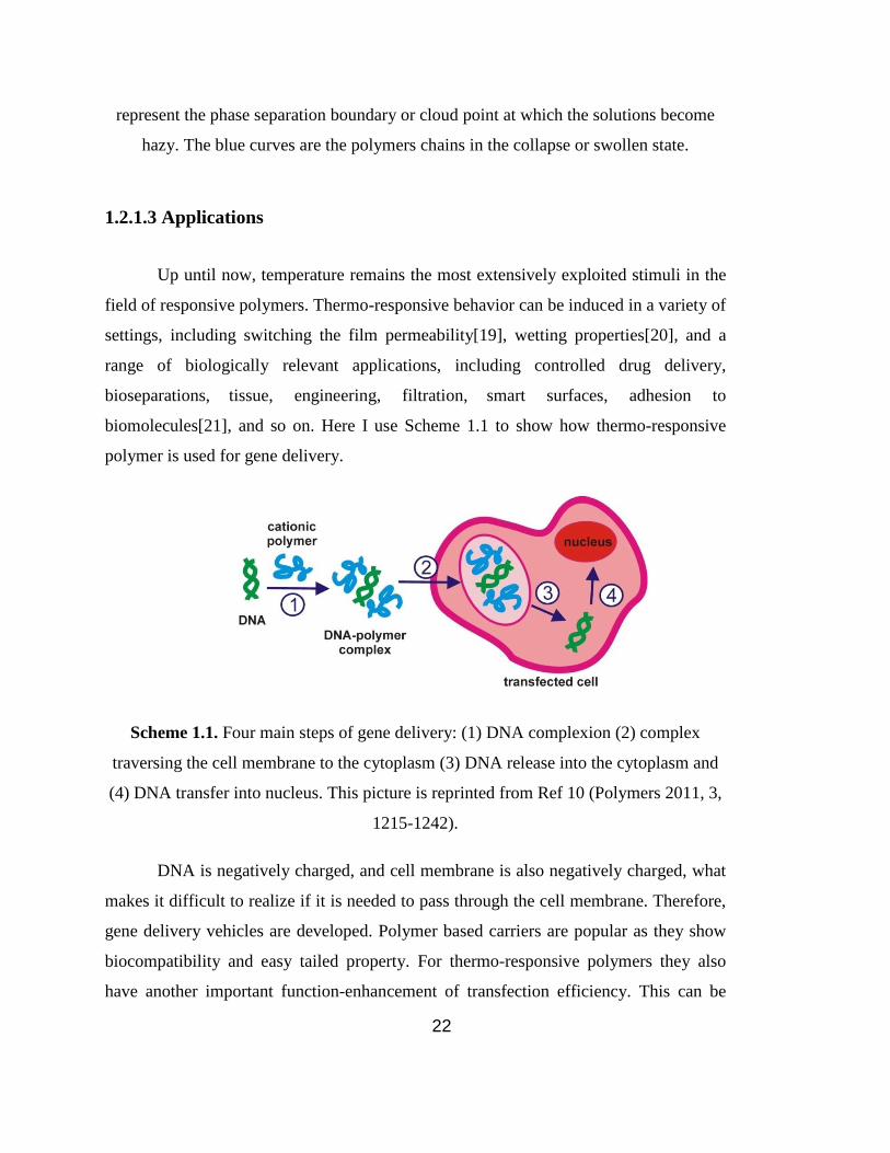
configuration. As different cells in vivo require different acid-basic balanced solutions
[18], as shown in Table 1.1, it’s becoming extremely important to develop pH-
responsive polymers with biocompatibility and antibacterial activity for the biological
application.
Table 1.1. Summary the requirements of specific pH condition of the biological system.
This table is reprinted from Ref 18(Advanced Drug Delivery Reviews, 2006, 58, 1655–
1670).

24
1.2.2.1 Poly(2-diethylaminoethyl methacrylate)
Poly(2-diethylaminoethyl methacrylate) (PDEA) is a pH-responsive polymer
with biocompatibility and low toxicity.[23]
PDEA shows controlled molecular weights,
well-defined chain ends, different macromolecular architectures and functionalities.[24]
The pKa of PDEA is around 7.3, depending on molecular weight. Different architectures
like block, star, and graft, can be realized by controlled radical polymerization such as
atom transfer radical polymerization (ATRP) and reversible addition fragmentation
transfer (RAFT).
In aqueous solutions of both star-shaped and linear PDEA, the cloud
point can be readily tuned by changing the pH of the solution and the molecular weight
and concentration of the polymer. Figure 1.5 shows the molecular structure of PDEA.
Due to its properties, it is used as a promising material in systems for the design and
precise synthesis of advanced synthetic biomaterials in gene delivery, pH-responsive
controlled release, etc.
Figure 1.5. The structure of PDEA.
1.2.2.2 Applications
pH-responsive polymeric systems have been extensively studied from both the
theoretical and applied perspectives.[23] Well-defined block copolymers resulting in the
formation of nanostructured particles or polymeric brushes can be produced with
controlled polymerization techniques. In aqueous homopolymers systems, external pH
could induce phase separation; in microgels, external pH could induce
swelling/deswelling of particles; for block copolymers, pH difference would result in the

25
pH-responsive polymers self-assemble into aggregates of different shapes. Because of
the easy configuration transition and biocompatibility of pH-responsive polymers, they
show wide application in biological fields, such as drug delivery systems, enzyme
immobilization, separation, chemo-mechanical systems, chemical valves, sensors,
controlled releases and so on. [18, 23, 25]
1.2.3 Other stimuli-responsive polymers
Besides the thermo- and pH-responisve polymers, there are also polymers that
can response to other stimuli, like voltage, light-irradiation,
or mechanical stress. In
general, physical stimuli include light, pressure, etc. Among the chemical stimuli, pH
value, the ionic strength, as well as the addition of chemical agents, are the most
common examples. Moreover, responses to antigens, enzymes, ligands or other
biochemical agents are biochemical stimuli-responsive polymers. Nowadays, the
stimuli-responsive polymers are explored for their various applications including drug
release, smart and self-healing coatings, tunable catalysis, biointerfaces, bioseparation
and responsive filters. [5]
1.2.4 Morphology of stimuli-responsive polymers
As mentioned above, stimuli-responsive polymers can perform conformation
changes on receiving an external signal change, like temperature, chemical composition,
irradiation with light, etc. In order to study the architectures and fundamental
approaches of stimuli-responsive polymers, generally the systems can be divided to two-
dimensional and three-dimensional.[5] Films are the most typical and commonly used
morphology in two-dimensional systems, including homopolymer brushes, block
copolymers brushes, mixed polymer brushes, hybrid film brushes, and so on. In three-
dimensional systems, particulates and their assemblies are the main part. In the
following subchapter, I will introduce stimuli-responsive polymer in each system and
how the transition changes exposed to the external stimuli.

26
1.2.4.1 Films
Films are the most commonly used morphology for the stimuli-responsive
polymers. Polymer brushes, layer by layer films, hydrogel films are the main
morphologies.[9] For polymer brush, one chain-end is fixed onto a solid substrate and
the other side is relatively flexible and can respond to the external stimuli. Up until now,
people use versatile methods to probe films such as contact angle, atomic force
microscopy, ellipsometry, quartz-crystal micro-balance, infrared and neutron
reflectivity. Original theories suggested that the density of the polymer chains was
constant[26, 27] but later a more accurate representation with a higher density of
monomer units at the substrate compared to the surface is introduced, as shown in
Figure 1.6b. [28] This distinction of polymer brushes is crucial in their applications,
because for the bulk transition or the surface they would behave differently and bring
different results.
Figure 1.6. Generalized depictions of density in polymer brushes which are grafted onto
the solid substrate. (A) Average chain density on the substrate; (B) denser chains close
to the substrate.
Moreover, the density of the polymer on the substrate would also have an impact
on the transition of the polymer, as shown in Figure 1.7[14]. A distinct transition exists
between very lightly grafted polymers in the ‘mushroom’ regime compared to the
densely packed ‘brush’ regime. The brush regime appears when the distance between
grafting sites of the polymers is greater than twice the radius of gyration (Rg) of the
individual polymers. In the mushroom regime, as the chain intensity is relatively low,

27
the interaction between solvent and substrate can’t be ignored. Therefore, a direct
consequence of this is that the hydrophilicity/hydrophobicity of the polymer corona is
therefore influenced by the nature of the underlying substrate.
Figure 1.7. Effect of polymer brush morphology on conformation transitions above
their LCST. Rg is the radius of gyration of an individual polymer chain. This picture is
reprinted with permission from Ref 14.
Besides polymer brush films, network film and porous gel films are also well
studied. Nanostructured thin network films are materials in which surface confinement
brings a range of opportunities for engineering stimuli-responsive properties. An
important attribute of gel thin films is their fast kinetics of swelling and shrinking
compared with bulk gels, ranging from microseconds to seconds. The swelling-response
of these films is highly anisotropic, because the attachment of the network to a surface
prohibits in-plane swelling. Another important attribute of films are porous thin gel
films. Switching between open and closed pores in thin gel films on shrinking and
swelling, respectively, provides a unique opportunity for the regulation of transport
through the film in a very broad diffusivity ranging from the level in solution down to a
level in solids.

28
Moreover, polymer film can not only be grafted onto the flat solid surface but
also grafted onto the well-defined and functional solid structure by different living
radical polymerization. This guarantees the polymer with bigger flexibility. It’s
interesting to see how the polymer behave when the environment changes, and whether
it would be different with different morphology such as free chain, onto nanoparticle or
on the network.
In summary, films have obvious advantages compared to bulk morphology.
First, fast responsiveness of tuning and switching adhesion between stimuli-responsive
materials, proteins and cells has been explored for the control of cell and protein
adhesion, which can be used for tissue engineering and bioseparation. Second, the
possibility of dynamic control of the permeation of chemicals through nanoporous
membranes interaction of biomolecules and ions with responsive surfaces offers a
unique opportunity for bioseparation. For example, surface-grafted stimuli-responsive
polymers provide an exciting means for controlling drug permeation through nano- and
microporous membranes.
1.2.4.2 Particles
Particles are a widely use morphology for stimuli-responsive polymers. In
general, there are two kinds. One kind is hybrid inorganic-polymer particles, which are
composed of an inorganic or metal particle core and a polymer shell showing intriguing
properties; the other kind is composed by various polymer types which can form
versatile assemblies. For the polymers assembly, as one block shows responsive
property exposing the stimuli, the swelling or contraction happens and may also induce
the reversible or irreversible structural transformation among vesicles, micelles,
nanogels, and so on.[6] Figure 1.8 shows the possible transformations of poly(ethylene-
alt-propylene)-b-poly(ethylene oxide)-b-poly(N-isopropylacrylamide) (PEP-PEO-
PNIPAM) composing triblock copolymers.[29]

29
Figure 1.8. Effect of block sequence in a triblock copolymer assembly structural
transformations. Reprinted with permission from Ref 29. Copyright (2011) American
Chemical Society.
When polymer chains are densely tethered to the surface of particles, one end of
the chain is covalently bonded, and the other side of the chain tries to stretch away from
the grafting sites and extend its conformation due to the excluded volume interaction,
hairy nanoparticle are generated. In particular, immobilization of polymers onto
nanoparticles to form a responsive corona offers potential in a wide range of
technological, biological and medical applications where the interfacial properties are
being modulated. This includes reducing non-specific protein binding, improving
biocompatibility, preventing coagulation/aggregation, enabling sensing capabilities or
modulating solubility. Hairy particles are one of the most widely used morphologies,
due to their applications in drug release, catalyst supports, smart particulate emulsifiers,
foam and liquid marble stabilizers, etc.
When grafting polymer chains onto the nanoparticle, the density onto the particle
would have an impact on the cloud point of the polymer, which shows the same result
compared to the film morphology. It has also been reported that the particle size would
also effect on the transition temperature, this can be explained by the reason that the

30
density of the polymer is dependent on the degree of curvature. Figure 1.9[14] show the
schematically curvature dependent polymer chain density, under the assumption that the
chain is homogeneously grafted onto the nanoparitcle.
Figure 1.9. (A) Polymer chains grafted onto the nanoparticle with different diameter.
(B) Calculated volume/chain as a function of nanoparticle radius. This picture is
reprinted from Ref 14.
1.2.4.3 Other morphologies
Besides particle and film, many other morphologies are also widely investigated,
like polymer brush layers, core-shell nanoparticles, capsules, lipid layers, hydrogels,
capsule and micelle, etc. Versatile morphologies provide more possibility to investigate
the stimuli-responsive polymers using different characterization methods such as atomic
force microscopy (AFM), quartz crystal micro-balance (QCM), contact angle (CA)
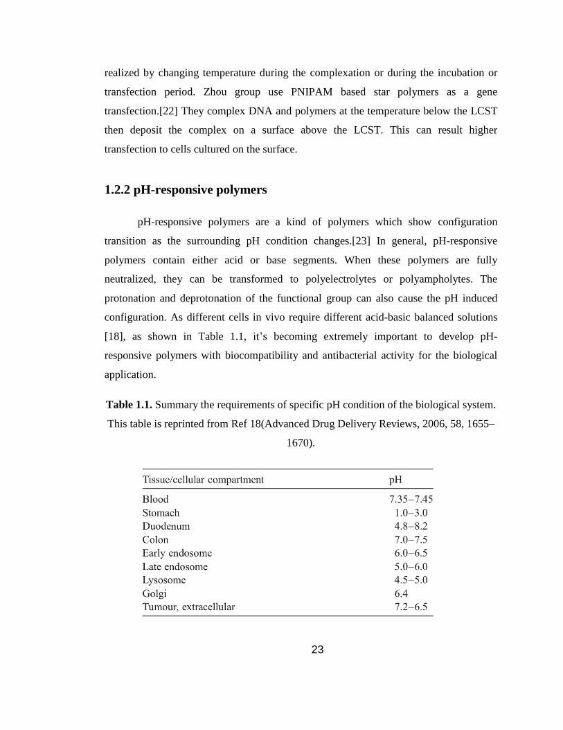
measurements, nanomechanical vantilever sensors, and so on.[30-32] Figure 1.10[5]
displays the main morphologies used. Contributing to the versatile morphologies
stimuli-responsive polymer can be used for many diverse applications, including drug
delivery[33], smart biointerfaces[34], sensors[35], self-healing coatings[36], tunable
catalysis[37], etc. For example, Nagasaki’s team prepared nanogels, which are
composed of a crosslinked, pH-sensitive polyamine core and conjugated PEO chains
surround. These nanogels can be taken by cells through receptor-mediated endocytic
31
pathways. In the acidic endosome, the nanoparticles swell and release drugs reserved in
the particle core.[38]
Figure 1.10. ‘Galaxy’ of nanostructured stimuli-responsive polymer materials. This
picture is reprinted from Ref 5.
1.3 Motivation
Nowadays controlling the diffusion of penetrants in solution and nanostructured
environments becomes a hot topic in colloid and polymer science. For this purpose
different characterization methods are developed to study the diffusion, such as forces
Rayleigh scattering (FRS)[39], fluorescence recovery after photobleaching (FRAP)[40],
pulse-field-gradient NMR (PFG-NMR)[41], dynamic light scattering (DLS)[42], quasi-
elastic neutron scattering (QENS)[43], etc. All these techniques have their own
advantages and also some limitations. Generally they require high concentration of the
diffusants in order to get high signal to noise ratio, but the high concentrations may

32
restrict the free diffusion behavior. Moreover, some specific task could be hard to
realize with a given technique. Take DLS for example, the polarizability determines the
extent of scattering and varies weakly with molecular structure, so DLS is not useful for
measuring the progress of chemical reactions or for following the motion of a specific
type of molecule at high dilution.
The theme of this thesis is to explore ways to control the diffusion (mobility) not
only in solution but also in nanostructured environment. Stimuli-responsive polymers
are ideal materials to construct the responsive species or the responsive environment for
mobility control. As stimuli-responsive polymers show instant response under external
stimuli, this would also bring the instant mobility change, thus an accurate and
quantitative monitoring of the species is required to record the changing process. In this
respect, fluorescence correlation spectroscopy (FCS) that is a powerful technique for
studying the dynamics of fluorescent species in various environments offers an
interesting alternative.[44] The fluorescent intensity fluctuations caused by the diffusion
of the species through a very small confocal detection volume are recorded and the
change process can be recorded. Because of its extremely small detection volume (V<
10-15
L), high sensitivity is reached and even single molecule can be traced in the
solution. Up until now, FCS has also found many applications in polymer and colloid
science.[45-47] Furthermore, the method was applied to investigate stimuli-responsive
polymer systems. For example, the pH or salt concentration induced changes in the size
of individual polymer chains[48, 49], or in the interaction between small molecules and
grafted polyelectrolyte brushes[50, 51], as well as, the temperature responsiveness of
Poly(N-isopropylacrylamide) (PNIPAM) microgel particles[52], and grafted hydrogel
films[53, 54] were studied.
In my thesis, I describe two approaches of using stimuli-responsive polymers to
control the diffusion behavior, as exhaustively described in chapter 3 and 4. In both
cases I used FCS as a technique to monitor and quantify the diffusion processes. The
basics of the FCS techniques are discussed in chapter 2.

33
CHAPTER 2
Methods
2.1 Principle of fluorescence correlation spectroscopy (FCS)
Fluorescence correlation spectroscopy (FCS) is a powerful technique for
studying the dynamics of fluorescent species such as small molecules, macromolecules,
or nanoparticles in various environments.[55] In an FCS experiment the fluorescent light
originating from a small probing volume formed around focused laser beam is detected.
When a fluorophore diffuses into this volume fluorescent photons are emitted and
detected due to multiple excitation-emission cycles from the fluorophore. When the
fluorophore diffuses out of the volume the emitted photons disappear. In this way the
diffusion of fluorophores causes time-dependent fluctuations in the detected
fluorescence intensity. By correlation analysis of these fluctuations, one can determine
the diffusion coefficient of the fluorophores. The time-dependent intensity fluctuations
can be induced not only from translational or rotational diffusion, but also from photo-
physical processes or chemical reactions that change the quantum efficiency of the
fluorophores. Thus, FCS can be also used for studying such processes.
The FCS technique was first introduced by Madge, Elson and Webb in 1972[56,
57], who applied it to measure diffusion and chemical kinetics of DNA- Ethidium
bromide (EtBr) intercalation. However, because of low detection efficiency, large
probing volume (~nL) results in large ensemble numbers and insufficient background
suppression, these early measurements show poor signal-to-noise ratios. Later, Rigler
and his coworkers[58] made a breakthrough by combining the FCS technique with
confocal detection that reduced the probing volume to ~fL. This combined with the use
of very sensitive avalanche photodiode detectors made the measurements of single

34
molecule trace in bulk solution possible and pave the way for the wide application of the
FCS. Figure 2.1 shows the typical modern FCS setup[59]. In order that only the few
fluorophores within the illuminated region are excited, a pinhole is also introduced to
block all light not coming from the focal region, which limits the detection volume also
in axial direction.
The excitation light is reflected by a dichroic mirror and focused into the sample
by a high numerical aperture objective (ideally NA > 0.9) to a diffraction limited spot.
The emitted light is collected by the same objective and passes through the dichroic
mirror. Here the dichroic mirror acts so that the emission wavelength can be passed
through and the excitation wavelength will be reflected. After passing through an
emission filter and a confocal pinhole, the emitted light is detected by an avalanche
photodiode detector (APD). Moreover, the confocal pinhole blocks the out-of-focus
fluorescence and only the fluorescence from diffusants in the confocal observation
volume can be detected. The confocal observation volume can be well approximated
[58] with a 3D Gaussian ellipsoid with radial and lateral dimensions of r0 and z0
respectively.

35
Figure 2.1. Scheme of a fluorescence correlation spectroscopy (FCS) setup.[59]
Here, I introduce the theoretical concepts how FCS works. As the fluorescent
species diffuses through the confocal observation volume, the fluorescence fluctuations
are produced, as shown in Figure 2.2[59]
δF(t) = F(t) − <F(t)> (2.1)
<F> is the average intensity. The normalized autocorrelation function is defined
as
𝐺(𝜏) =<𝛿𝐹(𝑡)𝛿𝐹(𝑡+𝜏)>
<𝐹(𝑡)>2 (2.2)
In the simplest case when the intensity fluctuations are caused only by the
diffusion of identical fluorescence molecules, the autocorrelation function describes the
probability that a fluorescent molecule that was in the confocal volume V at time t will
Objective
Dichroic
mirror
Emission Filter
Exciting Laser
Sample
Lens
Objective
Dichroic
mirror
Emission Filter
Exciting Laser
Sample
Lens
APD
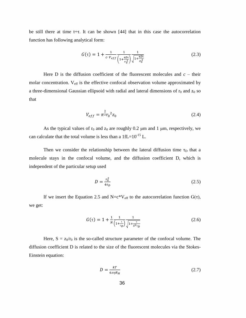
36
be still there at time t+τ. It can be shown [44] that in this case the autocorrelation
function has following analytical form:
𝐺() = 1 +1
𝑐 𝑉𝑒𝑓𝑓
1
(1+4𝐷
𝑟0 2 )
1
√1+4𝐷
𝑧0 2
(2.3)
Here D is the diffusion coefficient of the fluorescent molecules and c – their
molar concentration. Veff is the effective confocal observation volume approximated by
a three-dimensional Gaussian ellipsoid with radial and lateral dimensions of r0 and z0 so
that
𝑉𝑒𝑓𝑓 = 𝜋3
2𝑟02𝑧0 (2.4)
As the typical values of r0 and z0 are roughly 0.2 μm and 1 μm, respectively, we
can calculate that the total volume is less than a 1fL=10-15
L.
Then we consider the relationship between the lateral diffusion time τD that a
molecule stays in the confocal volume, and the diffusion coefficient D, which is
independent of the particular setup used
𝐷 =𝑟0
2
4𝜏𝐷 (2.5)
If we insert the Equation 2.5 and N=c*Veff to the autocorrelation function G(τ),
we get:
𝐺() = 1 +1
𝑁
1
(1+
𝐷)
1
√1+
𝑆2𝐷
(2.6)
Here, S = z0/r0 is the so-called structure parameter of the confocal volume. The
diffusion coefficient D is related to the size of the fluorescent molecules via the Stokes-
Einstein equation:
𝐷 =𝑘𝑇
6𝑅𝐻 (2.7)

37
Where k is the Bolzmann constant, T is the absolute temperature, η is the
viscosity of the medium and RH is the hydrodynamic radius of the molecule.
Figure 2.2. Fluorescence fluctuations caused by diffusing fluorescent species coming in
and out of the observation volume.[59]
2.2 FCS experimental setup
The FCS measurements described in my thesis were performed on a commercial
setup (Carl Zeiss, Germany) consisting of the modules LSM510, ConfoCor 2 and an
inverted microscope model Axiovert 200 with a C-Apochromat 40×, NA 1.2 water
immersion objective. Depending on the studied fluorophores the excitation was done
either with an argon laser (488 nm) combined with a LP505 long pass emission filter or
with a HeNe laser (633 nm) combined with a LP650 long pass filter. For detection an
avalanche photodiode operating in single photon counting mode was used. Aqueous
dispersions and solutions were studied either in 8-well, polystyrene chambered cover
glass (Laboratory-Tek, Nalge Nunc International) or in an Attofluor cell chamber (Life
Technologies) in which a microscope cover glass supporting the inverse opal structure

38
was mounted. For each studied sample series of 15 measurements with a total duration 5
min were performed. The experimental autocorrelation function was obtained by single
photon counting, followed by binning and correlating using the commercial (Carl Zeiss)
software correlator of the setup. The recorded experimental autocorrelation functions
were fitted using the system software (Carl Zeiss) with the following analytical function:
(2.8)
Here, the first term represent the so called triplet state dynamics and, fT and τT
are the fraction and the decay time of the triplet state, of the species, and S is the so-
called structure parameter, S = z0/r0. The fits yielded the diffusion time τD and through
Equation 2.5 the diffusion coefficient D of the studied fluorescent species. Next, the
hydrodynamic radius RH was calculated (assuming freely diffusing spherical particles)
using Equation 2.7 RH = kBT/6πηD. Furthermore, the molar concentration c=N*Veff of
the studied species and their molecular (or particle) fluorescent brightness <F(t)>/N
were also determined. As the dimensions r0 and z0 of the confocal observation volume
are not known a priori they were determined by performing calibration experiments
using a fluorophore with known diffusion coefficient, e.g. Alexa 488 and 647 in
water[60].
2.3 Scanning electron microscopy
The silica inverse opal structure was characterized by scanning electron
microscopy (SEM) using a LEO Gemini 1530 microscope, at a voltage of 0.7 kV. For
the cross section images of inverse opal, the substrate is with 75o tilt angle to the
parallel.
DD
t
T
T
S
Ne
f
fG T
2
/
11
11
111)(

39
2.4 pH meter
The pH value of the studied solutions was measured by a Seven Excellence pH
meter from Mettler Toledo. Before pH measurement, pH meter was calibrated. Each pH
value in my thesis was obtained by averaging three independent measurements.
2.4.1 pH adjustment
pH was adjusted by adding HCl and NaOH solution for the PDEA/PS hairy
nanoparticle and PDEA single chain dispersion, and also in the confined environment.
In PNIPAM modified inverse opal project, buffer solution was used. For Alexa Fluor
647, HPCE buffer solution (pH 8.0) from Sigma Aldrich is directly used; for the QD
525 with amino group, citrate buffer (pH 4.0) from Sigma Aldrich is directly used.
2.5 Gel permeation chromatography
Gel permeation chromatography (GPC) was used to determine molecular weight
of the polymer obtained from bulk polymerization, which is believed to be comparable
to the molecular weight of the chains grafted from surface. For GPC, PS was used as a
standard; DMF was used as an eluent.
2.6. Materials
2.6.1 Fluorescent dyes
Fluorescent dyes are defined also as fluorescent molecules or fluorochromes. In
1933, Polish scientist Jablonski[61] publish one paper discussing how fluorescence is
produced, as shown in Figure 2.3. The electrons in fluorescent dyes are normally in the
ground singlet state. As fluorescent dyes adsorbs matched photon from outside, the

40
electrons can be excited to higher singlet state and return back to the ground singlet
state, at the same time energy would release as fluorescent emission. The adsorption
process last 10-15
s, which can be neglected as it occurs much faster than other
transitions; the fluorescent emission process has the interval of 10-9
-10-12
s. For these
two processes we regard them as simultaneously happen. As there would be unavoidable
energy loss like heat, the photon released would have a longer wavelength compared to
the one adsorbed by the fluorescent molecules, so fluorescent dye adsorb one photon
with higher energy and emit one photon with lower energy. But it can be also possible
that the excited electron enter excited triplet state and then returns to ground singlet
state, at the same time energy would release as phosphorescence. This process has
interval of 102-10
-2 s. As we can see that the lifetime of phosphorescence is quite long
and phosphorescence quantum yield from the triplet state is very low, it is regarded as
no luminescence. For qualified fluorescent dyes for FCS, high fluorescence efficiency
and low triplet fraction are required. In practical application of fluorescent dyes, the
environment would have also an important impact on the fluorescence efficiency, as
triplet-state is dependent on the illumination intensity, concentration of molecular
oxygen and some heavy metals or halogen ions. So for FCS measurements, we should
choose fluorescent dyes with the high quantum efficiency, large absorption section and
photostability.
Figure 2.3. Jablonski diagram schematic illustration the generation process of
fluoresce and phosphorescence.

41
2.6.1.1 Alexa series
Alexa Fluor dyes are synthesized through sulfonation of coumarin, rhodamine,
xanthene (such as fluorescein), and cyanine dyes. Sulfonation makes Alexa Fluor dyes
negatively charged and hydrophilic. Usually Alexa series are the most commonly used
dyes as they own less pH sensitivity, photo stability and bright comparisons. Moreover,
the excitation and emission spectra of the Alexa Fluor series cover the visible spectrum
and extend into the infrared, which broaden its application area. Alexa series is a
suitable candidate for FCS measurement. Fig 2.4a shows the structure of Alexa 488 and
2.4b is its adsorption and fluorescence spectra[62], 2.4c shows the structure of Alexa
647 and 2.4d is its adsorption and fluorescence spectra[63].
Figure 2.4. (a) Molecular structure of Alexa 488 and (b) its absorption and fluorescent
emission spectra[62]; (c) Molecular structure of Alexa 647 and (d) its absorption and
fluorescent emission spectra[63].

42
2.6.1.2 Bodipy
Bodipy is the abbreviation of boron-dipyrromethene, which is a kind of
fluorescent dyes. Bodipy is composed of dipyrromethene complexed and a disubstituted
boron atom, typically a BF2 unit. The core part is 4,4-difluoro-4-bora-3a,4a-diaza-s-
indacene (Figure 2.5a) and normally it is decorated with other functional group for
different use.[64] Bodipy is a bright, green-fluorescent dye with similar excitation and
emission to fluorescein or Alexa Fluor. It has a high extinction coefficient and
fluorescence quantum yield and is relatively insensitive to solvent polarity and pH
change, in addition it can’t be dissolved in water solution, so it’s an ideal dye for the
pH-responsive system. Figure 2.5b is the molecular structure of 4,4-difluoro-5,7-
dimethyl-4-bora-3a,4a-diaza-s-Indacene-3-propionic acid, succinimidyl ester from Life
Technologies we are using in this thesis, and Figure 2.5c shows its absorption and
fluorescent emission spectra[65].
Figure 2.5. (a) Molecular structure of Bodipy core, (b) Molecular structure of Bodipy
used in this thesis and (c) its absorption and fluorescent emission spectra[65].
43
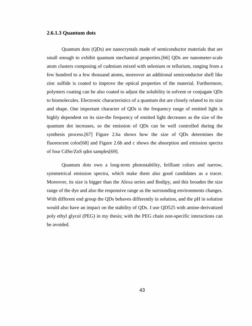
2.6.1.3 Quantum dots
Quantum dots (QDs) are nanocrystals made of semiconductor materials that are
small enough to exhibit quantum mechanical properties.[66] QDs are nanometer-scale
atom clusters composing of cadmium mixed with selenium or tellurium, ranging from a
few hundred to a few thousand atoms, moreover an additional semiconductor shell like
zinc sulfide is coated to improve the optical properties of the material. Furthermore,
polymers coating can be also coated to adjust the solubility in solvent or conjugate QDs
to biomolecules. Electronic characteristics of a quantum dot are closely related to its size
and shape. One important character of QDs is the frequency range of emitted light is
highly dependent on its size-the frequency of emitted light decreases as the size of the
quantum dot increases, so the emission of QDs can be well controlled during the
synthesis process.[67] Figure 2.6a shows how the size of QDs determines the
fluorescent color[68] and Figure 2.6b and c shows the absorption and emission spectra
of four CdSe/ZnS qdot samples[69].
Quantum dots own a long-term photostability, brilliant colors and narrow,
symmetrical emission spectra, which make them also good candidates as a tracer.
Moreover, its size is bigger than the Alexa series and Bodipy, and this broaden the size
range of the dye and also the responsive range as the surrounding environments changes.
With different end group the QDs behaves differently in solution, and the pH in solution
would also have an impact on the stability of QDs. I use QD525 with amine-derivatized
poly ethyl glycol (PEG) in my thesis; with the PEG chain non-specific interactions can
be avoided.

44
Figure 2.6. (a) Five different nanocrystal solutions excited with the same long-
wavelength UV lamp.[68] (b) Absorption and (c) emission spectra of four CdSe/ZnS
qdot samples.[69].
2.6.2 Silica inverse opals
Silica inverse opal is a three-dimensional ordered structure which is consisting of
regular spherical voids with interconnecting circular pores, and the silica wall made it
with good mechanical stability.

45
2.6.2.1 Silica and PS nanoparticles
Silica was purchased from Sigma Aldrich with 30% concentration and diameter
of 7 nm and used as received; PS nanoparticle (1 μm, 330 nm and 200 nm in diameter)
were synthesized according to the literature.[70] Round microscope glass slides with
diameter of 25 mm and thickness of 170 μm, were purchased from Menzel, Germany
and cleaned with a 2% Hellmanex solution (Hellma, Germany) prior to further use.
2.6.2.2 Preparation
Inverse opals structures on a thin glass slide substrate were prepared as described
in details elsewhere.[71-74] Briefly the substrate was lifted with 400 nm/s lifting speed
from a mixed aqueous dispersion of 1.5 wt% PS particles and 0.3 wt% silica
nanoparticles at 20 oC environmental temperature and 50% RH environmental humidity
as measured. As we only want one side of the substrate is coated with inverse opal
structure, the opposite side is coated with polyethylene film which blocks the contact of
mixture dispersions and the substrate. Schematic illustration of the fabricating process is
shown in Figure 2.7.

46
Figure 2.7. Scheme of the vertical lifting deposition of mixture dispersions of
PS nanoparticle and SiO2 nanoparticles.
The polyethylene film on the other side of the substrate is peeled off before high
temperature calcination. The PS template was removed by pyrolysis in air at 500 oC for
5 hours, leaving the silica nanoparticle stacked and fused in an ordered three-
dimensional structure, shown in Figure 2.8.
Figure 2.8. Preparation of silica inverse opal by high temperature calcination.
Following this method, we can get ordered three-dimensional inverse opal
structure. Figure 2.9 show the SEM images from top view and side view of silica

47
inverse opal made from dispersions of silica nanoparticle and PS nanoparticle with
diameter of 200 nm, 300 nm and 1µm, respectively.
Figure 2.9. Scanning electron microscopy images of inverse opals made from (a)
200 nm, (b) 300 nm, (c) 1 μm polystyrene particles in diameter.

48
2.6.3 PS/PDEA hairy nanoparticles and PDEA single chains
… provides us the PS/PDEA hairy nanoparticle and PDEA single chain. To
enable the fluorescence, the BodipyBODIPY is covalently bounded to the PS/PDEA
hairy nanoparticle and PDEA chain. Detailed synthesis processes are described in our
paper.[75]
2.6.4 Cells for FCS measurement
For the FCS measurements in solution, 8-well chambers from Nunc Lab-Tek
were used. For the FCS measurement in the inverse opals, an Attofluor cell chamber
(Invitrogen, Leiden, Holland) was used as a sample cell, in which one glass slide with
25 mm in diameter and 170 μm in thickness is mounted, and the diluted dye solution is
deposited on top to cover the inverse opal coated glass slide totally, on top of the whole
cell another clean glass slide is added to prevent the water vapor condensed at the
detection camera lens. Figure 2.10 show 8-well chamber (a)[76] and the Attofluor cell
chamber (b)[77]. To study the temperature dependence of nanoparticle mobility by FCS,
an extra commercial heating setup is added, which is shown in Figure 2.10c.

49
Figure 2.10. (a) 8-well chamber[76]. (b) Attofluor cell chamber[77] and (c) Scheme of
the heating setup.
2.7 Atom transfer radical polymerization (ATRP)
Free radical polymerization is one kind of polymerization methods by
continually adding free radical building block to form polymer. Because it requires
relatively non-specific nature of free radical chemical interactions, it becomes one of the
most versatile methods to obtain a wide variety of different polymers and materials
composite. Among the radical polymerizations, reversible deactivation radical
polymerization are the most popular used, which includes atom transfer radical
polymerization (ATRP), reversible addition-fragmentation chain transfer polymerization

50
(RAFT) and stable free radical polymerization (SFRP).[78, 79] Among these methods
ATRP are well used for surface initiated polymerization. Here, I would take ATRP for
example to introduce the mechanism and the polymerization condition.
ATRP was independently discovered by Mitsuo Sawamoto [80] and Jin-Shan
Wang and K. Matyjaszewski [81, 82] in 1995. ATRP is controlled by equilibrium
between propagating radical and dormant species.[83] For ATRP, it can be divided into
three steps: initiation stage, propagation stage and end stage.[84]
Initiation stage:
R-X is alkyl halides, which is used as the initiator, CuX is on behalf of redox-
active transition metal complexes; ligand, whose electronic effect and steric effect
would have an important impact on the activation and deactivation activity of the
catalyst. Cu(I) is the activator, R is the radical, CuX(II) is the deactivator, P is the
growing radical.
Propagation stage:
Pn-X is activated by CuX/ligand to become radical, and more monomers can be
grown on the active radical to get large molecular weight.
Termination stage:
51
Two radical grow together to terminate the polymerization.
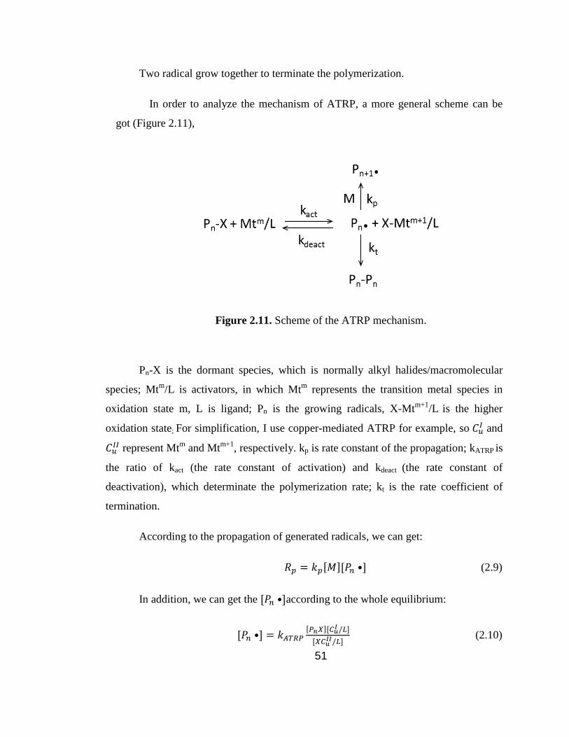
In order to analyze the mechanism of ATRP, a more general scheme can be
got (Figure 2.11),
Figure 2.11. Scheme of the ATRP mechanism.
Pn-X is the dormant species, which is normally alkyl halides/macromolecular
species; Mtm
/L is activators, in which Mtm
represents the transition metal species in
oxidation state m, L is ligand; Pn is the growing radicals, X-Mtm+1
/L is the higher
oxidation state; For simplification, I use copper-mediated ATRP for example, so 𝐶𝑢𝐼 and
𝐶𝑢𝐼𝐼 represent Mt
m and Mt
m+1, respectively. kp is rate constant of the propagation; kATRP is
the ratio of kact (the rate constant of activation) and kdeact (the rate constant of
deactivation), which determinate the polymerization rate; kt is the rate coefficient of
termination.
According to the propagation of generated radicals, we can get:
𝑅𝑝 = 𝑘𝑝[𝑀][𝑃𝑛 •] (2.9)
In addition, we can get the [𝑃𝑛 •]according to the whole equilibrium:
[𝑃𝑛 •] = 𝑘𝐴𝑇𝑅𝑃[𝑃𝑛𝑋][𝐶𝑢
𝐼 /𝐿]
[𝑋𝐶𝑢𝐼𝐼/𝐿]
(2.10)

52
Insert Equation 2.10 to 2.9, we can get:
𝑅𝑝 = 𝑘𝑝[𝑀][𝑃𝑛 •] = 𝑘𝑝𝑘𝐴𝑇𝑅𝑃[𝑃𝑛𝑋][𝐶𝑢
𝐼 /𝐿][𝑀]
[𝑋𝐶𝑢𝐼𝐼/𝐿]
(2.11)
From Equation 2.11 we could see that Rp depends on the catalyst activity
(KATRP), concentration of monomer, the redox-active transition metal complexes.
Moreover, ligand species, monomer/dormant species, and the reaction condition
(solvent, temperature, pressure, etc.) would also have an impact on the polymerization
rate. Once the initiator is added, all the monomer can be immediately activated, and the
chain can grow at the same time, so the low molecular weight polydispersity can be got.
If the transfer and termination are negligible, the degree of polymerization can be
calculated:
𝑋 = [𝑀0]
[𝐼0] (2.12)
[𝑀0] is the monomer concentration, [𝐼0] is the initiator concentration. But we
need to pay attention that during the polymerization process, the generated radicals can
react not only with monomer but also with other generated radicals, which means that
the termination occurs at the same time. Here we need to compare kp and kt. As kdeact is
much larger than kact, for most of the monomer are in the dormant species, and the
concentration of radical is low, the generated oxidized metal complexes, X-Mtm+1
/L acts
at persistent radicals to reduce the stationary concentration of growing radicals and
minimize the concentration of termination. Typically in a well-controlled ATRP, people
can get a small amount of terminated chains but a uniform growth of all the chains with
low molecular weight polydispersity (𝑃𝐷 =𝑊𝑚
𝑊𝑛) which is proximately between 1.0 and
1.5.
In the past years, different designed morphologies can be polymerized by ATRP,
like linear chains, block copolymers, cyclic structures, etc. Moreover, the dimensions
and dispersity can be also well controlled.[83] Figure 2.12 shows controlled topology
prepared by ATRP. As it provides a simple route for many well-defined (co)polymers

53
with predetermined molecular weight, narrow molecular weight distribution, and high
degree of chain end functionality, which broaden the substance field of stimuli-
responsive polymer in nature.
Figure 2.12. Polymers with controlled topology prepared by ATRP, reprinted
from Ref 76.
2.7.1 “Grafting from”
In general, the ATRP technique includes “grafting from” and “grafting to”
techniques. For the “grafting from” technique, firstly the initiators are fixed on the
substrate, then monomer propagates onto it and the polymer chains grow (Figure 2.13).
As the initiators can be fixed tightly by chemical reaction and monomer can diffuse
freely in the solution to the growing chain, high density of polymer brushes and low
poly dispersity can be obtained.
Figure 2.13. Graft of polymers from an initiator-functionalized substrate.
For the “grafting from” technique, the initiator groups can be successfully coated
onto both organic and inorganic materials, both flat and curved surfaces. As a

54
consequence, polymer brushes of varying composition and dimensions can be prepared
by surface-initiated growth from like on spheres, flat solid surface or colloids.[85]
2.7.2 “Grafting to”
The “grafting to” technique is also a widely used technique in ATRP. Usually
the monomers polymerize to the polymer chains in solution, and then the whole polymer
chains are grafted onto the substrate decorated with initiators. Compared to the
“grafting from” technique, “grafting to” leads to lower brush densities as it is limited
intrinsically by the excluded volume effects. As polymer brushes are sterically less
confined when they are prepared by the grafting to technique, it would broaden the
cloud point transition compared to highly dense polymer brushes.
Figure 2.14. Graft of polymer chains onto preformed substrate.

55
CHAPTER 3
Temperature controlled diffusion in PNIPAM
modified silica inverse opals
In this chapter, I report a new strategy for the preparation of well-defined and
mechanically stable porous nanostructures with tunable porosity. Silica inverse opals,
which are known as a model system for a porous periodic nanostructure, were grafted
with brushes of the thermo-responsive poly(N-isopropylacrylamide) (PNIPAM) grown
via atom transfer radical polymerization. By tuning the temperature I was able to control
the overall porosity of the system and thus the mobility of small penetrants.
Fluorescence correlation spectroscopy was used to directly monitor and in situ quantify
the changes in the penetrants’ mobility, which is caused by changes of polymers
conformation.
3.1 Introduction and motivation
Understanding and controlling the diffusion of small molecules, macromolecules
and nanoparticles in complex, nanostructured environments is of paramount
fundamental and technological importance. Often, diffusion is the dominant mechanism
for the transport of such species in e.g. solid nanoporous structures, polymer solutions
and gels or in living cells. Thus, it is relevant for many processes and applications
including drug delivery, cell nutrition, porous chromatography, polymer synthesis and
separation, treatment of waste water, oil recovery, etc. Not surprisingly therefore,
studying the penetrant diffusion and correlating it to the chemical, physical and
topological characteristics of the nanostructured environment has become a major
research topic in various fields spanning from polymer physics to cell biology. A number
of theories, models and empirical relations have been introduced to describe the

56
diffusion of small species in polymer systems, in intercellular matrices or in solid
periodic nanoporous structures.
From application point of view, the possibility for on demand control over the
diffusion of small penetrants in nanoporous structures is even more important. Indeed,
such possibility gives various opportunities as to e.g. control the drug release rate or to
select the relevant sizes in a separation process. Traditionally, control over the penetrant
diffusion is achieved by changing the size and/or density of the nanopores. However, in
a solid nanoporous structure, such as an anodized aluminum membrane, a porous glass
or a silica inverse opal, the pore size is determined during the fabrication process and
typically cannot be changed e.g. by applying an external stimulus. This is unfortunate,
as the solid nanoporous structures offer the mechanical strength and stability that is
required for most applications. Alternatively, in some polymer based nanoporous
systems such as e.g. hydrogels, the pore size and thus the penetrant diffusivity can be
controlled by tuning the temperature or the pH value. Hydrogels, however, lack
mechanical stability that often makes their application problematic.
In this chapter, I describe a new system combining the mechanical stability of a
solid nanoporous structure with the possibility for fine tuning offered by a thermo-
responsive polymer. As a solid support I used a silica inverse opal (iOpal), which is a
highly order porous structure, consisting of regular arrangements of spherical voids
surrounded by solid silica walls with interconnecting circular pores.[71-74] Due to their
well-defined nanoporous structure iOpals have been often used as model system to study
the diffusion of small molecules[86], nanoparticles[87] or DNA[88]. Here, in order to
add responsiveness and tunability to the nanoporous structure I modified the iOpal
interior surface with grafted poly(N-isopropylacrylamide) (PNIPAM) brushes by surface
initiated atom transfer radical polymerization (ATRP). The PNIPAM is one of the most
popular thermo-responsive polymers and exhibits a lower critical solution temperature
(LCST) of around 32 oC[15] i.e. close to the humans body temperature. In aqueous
solutions, below the LCST the PNIPAM chains are hydrated and adopt an extended coil
conformation, while above the LCST they are dehydrated and collapse to a globular
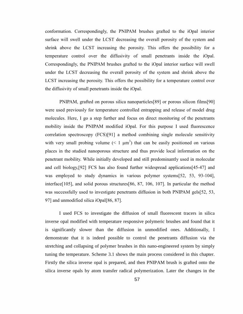
57
conformation. Correspondingly, the PNIPAM brushes grafted to the iOpal interior
surface will swell under the LCST decreasing the overall porosity of the system and
shrink above the LCST increasing the porosity. This offers the possibility for a
temperature control over the diffusivity of small penetrants inside the iOpal.
Correspondingly, the PNIPAM brushes grafted to the iOpal interior surface will swell
under the LCST decreasing the overall porosity of the system and shrink above the
LCST increasing the porosity. This offers the possibility for a temperature control over
the diffusivity of small penetrants inside the iOpal.
PNIPAM, grafted on porous silica nanoparticles[89] or porous silicon films[90]
were used previously for temperature controlled entrapping and release of model drug
molecules. Here, I go a step further and focus on direct monitoring of the penetrants
mobility inside the PNIPAM modified iOpal. For this purpose I used fluorescence
correlation spectroscopy (FCS)[91] a method combining single molecule sensitivity
with very small probing volume (< 1 µm3) that can be easily positioned on various
places in the studied nanoporous structure and thus provide local information on the
penetrant mobility. While initially developed and still predominantly used in molecular
and cell biology,[92] FCS has also found further widespread applications[45-47] and
was employed to study dynamics in various polymer systems[52, 53, 93-104],
interface[105], and solid porous structures[86, 87, 106, 107]. In particular the method
was successfully used to investigate penetrants diffusion in both PNIPAM gels[52, 53,
97] and unmodified silica iOpal[86, 87].
I used FCS to investigate the diffusion of small fluorescent tracers in silica
inverse opal modified with temperature responsive polymeric brushes and found that it
is significantly slower than the diffusion in unmodified ones. Additionally, I
demonstrate that it is indeed possible to control the penetrants diffusion via the
stretching and collapsing of polymer brushes in this nano-engineered system by simply
tuning the temperature. Scheme 3.1 shows the main process considered in this chapter.
Firstly the silica inverse opal is prepared, and then PNIPAM brush is grafted onto the
silica inverse opals by atom transfer radical polymerization. Later the changes in the

58
fluorescent species mobility caused by the different conformations of the PNIPAM
chains are studied by FCS.
Scheme 3.1. Scheme of temperature controlled diffusion in PNIPAM modified
silica inverse opals.
3.2 Atom transfer radical polymerization on silica inverse
opals
3.2.1 Preparation of the silica inverse opals
The silica inverse opals with the void diameter of 315 nm were fabricated by
vertical deposition (VD) method as described in Chapter 2. Typical scanning electron
microscopy (SEM) images of as prepared inverse opals are shown in Figure 2.9 in
Chapter 2. The inverse opal has a thickness of 5 microns with a void diameter and
interconnecting circular pores size of 315 nm and 105 nm respectively. In addition some
defects and cracks can be observed, which usually form during drying and calcination
process.[108, 109] However such cracks can be easily seen in laser scanning confocal

59
microscopy (LCSM) and in order to avoid contributions of tracer diffusion in cracks all
the FCS measurements were done in the center of continuous platelets (Fig 3.1).
Figure 3.1. Reflectance images of silica inverse opal taken with the confocal
microscope part of the FCS setup.
3.2.2 ATRP on silica inverse opals
Then the silica inverse opals were coated with PNIPAM chains using
“grafting-from” technique in ATRP.
3.2.2.1 Materials
N-isopropylacrylamide (NIPAM), CuCl, H2O2 (35%), methyl (S)-2-
chloropropionate, triethylamine (TEA) and anhydrous toluene were purchased from
Aldrich. NH3 (25%) was purchased from VWR Chemicals. Tris (2-dimethylaminoethyl)
amine was purchased from Alfa Aesar. TEA was distilled from CaH2, and the starter 3-
(2-bromoisobutyryl)propyl)dimethyl chlorosilane was synthesized following the
procedure described in the literature.[110] In order to prevent degradation by moisture,

60
the starter and TEA were both stored under argon atmosphere. NIPAM monomer was
recrystallized from hexane. The precipitate was rinsed with water, ethanol, and finally
with diethyl ether and dried in a vacuum oven for 24 h. Anhydrous toluene and tris (2-
dimethylaminoethyl) amine were used directly after purchased. All aqueous solutions
were prepared with ultrapure water purified with a Milli-Q UV-Plus water purification
system (Millipore, Bedford, MA). The water had a resistivity of >18 Mcm-1
.
3.2.2.2 Initiator immobilization
In order to prepare the silicon surface for the starter immobilization and to assure
controlled hydration state of the silicon oxide layer on top, a base cleaning was
performed. Silica inverse opal was immersed in a mixture of NH3 (4 mL, 25%), H2O2 (4
mL, 35%) and Millipore water (50 mL) for 2 hours at room temperature. Afterwards, the
silicon surface was rinsed with abundant amounts of Millipore water and dried with a N2
flow.
Then the freshly cleaned silica inverse opal was is immersed in mixed solution of
0.4 mL TEA, 0.2 mL 3-(chlorodimethylsilyl) propyl 2-bromo-2-methylpropanoate and
25 mL anhydrous toluene with stirring for 10 h under argon, and then wash with
dichloromethane placed in soxhlet apparatus for 6 hours and used for graft
polymerization.
3.2.2.3 Surface-initiated polymerizations
The surface-functionalized silicon substrate was placed in the tube and the reaction
solution was prepared in DMF/H2O (1:1, V = 28 mL) containing the monomer NIPAM
(m = 2.72 g), the ATRP catalyst CuCl (m = 19 mg) the ligand tris (2-
dimethylaminoethyl) amine (V = 55.8 μL) and sacrificial initiator 22 µL Methyl (S)-2-
chloropropionate. The polymerization mixture was carefully degassed through several
freeze-thaw cycles to remove dissolved oxygen and the polymerization was carried out

61
at room temperature. After 45 min reaction time the silica inverse opal was removed
from the polymerization mixture rinsed with dichloromethane and dried.
Subsequently, the glass slides were placed in a Soxhlet apparatus, continuously
extracted with methanol for 18 h, and dried under argon. The PNIPAM solid was
obtained by dialyzing the PNIPAM solution with the 1000 g/mol dialysis tube for 3 days
and then removing the solvent by one rotary evaporator, and GPC is used to determine
the molecular weight of PNIPAM. The number-average molecular weight (Mn) is 21000
g/mol, as shown in Figure 3.2.
Figure 3.2. Gel-permeation chromatography results of the polymer with Mn =21000
g/mol synthesized in solution. (a) Elugram of the PNIPAM chains. (b) Molecular weight
distribution.

62
Modified inverse opals were also analyzed with SEM and compared to
unmodified one (Figure 3.3). From SEM images we can see the presence of the polymer
layer grafted on the surface of the inverse voids, resulting in the pores between
interconnecting holes are getting smaller.
Figure 3.3. Inverse opals images before and after grafting PNIPAM chains.
Moreover, the optical image of inverse opal coated on the glass slide can also
show that PNIPAM chains are successfully grafted onto the inverse opal. As shown in
Figure 3.4, the color of the substrate is turning from green to red after being coated with
PNIPAM chains. For the right image we see that there is a small piece of green color,
this is because of it got in touch with the holder of the substrate which can’t be exposed
to the solution during the polymerization. These optical images are taken vertically from
the top. This structure color can be explained by Bragg’s law.[111]
Figure 3.4. Optical images of silica inverse opal coated substrate before and
after grafting PNIPAM chains.

63
3.3 Dyes and solvents for FCS measurement
Alexa Fluore 647 and QD 525 were purchased from Invitrogen (Karlsruhe,
Germany) and used as tracers. For the FCS measurement solutions of either Alexa
Fluore 647 with concentration ~5 nM in HPCE buffer (pH 8.0) or QD 525 with
concentration 20 nM in citrate buffer (pH 4.0) were used.
3.4 Alexa 647 and QD 525 diffusion in PNIPAM grafted silica
inverse opals
The FCS measurements were performed on a commercial setup (Carl Zeiss,
Germany) consisting of the modules LSM510, ConfoCor 2 and an inverted microscope
model Axiovert 200 with a C-Apochromat (40×, NA 1.2) water immersion objective. A
HeNe laser (633 nm) was used for exciting Alexa 647, and the emission was collected
after filtering with a LP650 long pass filter; an argon laser (488 nm) was used for
exciting QD 525, and the emission was collected after filtering with a LP505 long pass
filter. The fluorescent tracers solutions were studied either in 8-well, polystyrene
chambered cover glass or in an Attofluor cell chamber in which a microscope cover
glass supporting the inverse opal structure was mounted. Reflection mode imaging was
performed with the same objective (C-Apochromat 40×), using excitation at very low
intensity at the laser wavelength of 488 nm combined with a long pass LP 475 emission
filter.
First, I used FCS to study the effect of the grafted PNIPAM brushes on the
diffusion of the small molecular dye-Alexa Fluor 647 in the modified iOpal. It is
important to emphasize that due to the extremely small probing volume of the FCS (~1
µm in axial direction) the small fluorescent tracer diffusion studies can nicely capture
this gradient in film as thin as few micrometers only. Even though cracks are presented
among iOpal, they can be clearly visualized by confocal microscopy in reflection mode,

64
which helps to define the exact location in the iOpal for tracer mobility measurements
(Figure 3.1). In my experiments, the objective’s immersion medium was water with
refractive index n ≈ 1.33. For the water-filled PNIPAM modified inverse opal with silica
(n ≈ 1.45) and filling volume fraction of about 20%, the effective refractive index was n
≈ 1.36. Due to this small refractive index mismatch, the estimated error of the diffusion
in the inverse opals was less than 10%.[73, 87, 112] Thus the strong shift of the
autocorrelation curves for the inverse opal toward to longer times was caused by the
confinement, as discussed and theoretically rationalized before.[87]
Figure 3.5 shows a typical FCS autocorrelation curve measured in the middle of
an iOpal modified with PNIPAM with Mn = 21000 g/mol. The autocorrelation curves of
Alexa 647 measured in the iOpal and iOpal modified with PNIPAM chains are strongly
shifted to the longer lag times, reflecting significantly slower diffusion. Both curves can
be nicely fitted with Equation 2.8 yielding diffusion times of τd = 75 μs and τd = 122 μs
in the iOpal and in the iOpal modified with PNIPAM brushes, respectively. For
comparison the diffusion of the same tracer in bulk citrate buffer solution is even faster
with diffusion time τd = 56 μs (the circle solid line). In order to verify the reproducibility
of these results, FCS measurements were performed at various lateral positions in the
studied iOpal, which yielded very similar results.
10-5
10-4
10-3
10-2
10-1
0,0
0,2
0,4
0,6
0,8
1,0
Alexa 647 in solution
Alexa 647 in IO
Alexa 647 in PNIPAM IO
G(
)
/ s

65
Figure 3.5. Normalized autocorrelation functions obtained for Alexa Fluor 647
diffusing in HPCE buffer solution (•), in silica iOpal filled with HPCE buffer solution
(□) and in PNIPAM modified silica inverse opal with HPCE buffer solution (Δ). The
solid lines represent the corresponding fits.
In order to compare the diffusion rate with the molecular weight of PNIPAM
chains, I control the polymerization time and get shorter PNIPAM chains and lower
molecular weight. The Mn of the short chain is 3100 g/mol and polydispersity is 1.2
determined by GPC. Figure 3.6a is the elution volume for the PNIPAM chains and
Figure 3.6b is its molecular weight distribution. Figure 3.7c shows the autocorrelation
curves of Alexa 647 diffuse in iOpal, short chain grafted iOpal and long chain grafted
iOpal, and the short chain is sandwiched between the iOpal and long chain grafted
iOpal, showing that the length of PNIPAM can adjust the size of the hole and have an
effect on the mobility of Alexa 647 inside.

66
Figure 3.6. Gel-permeation chromatography results of the polymer with Mn =3100
g/mol generated in the solution. (a) Elugram of the PNIPAM chains. (b) Molecular
weight distribution. (c) Alexa 647 diffuses in bare iOpal and iOpal with different length
of PNIPAM chains. Alexa Fluor 647 diffuse in silica iOpal filled with HPCE buffer
solution (□) and in short PNIPAM chains modified silica iOpal (Δ) and in long
PNIAPM chains modified iOpal (◊). The solid lines represent the corresponding fits.

67
3.5 Tuning (controlling) the penetrant diffusion
Next I focus on the possibility to tune the diffusivity in the PNIPAM modified
iOpal by controlling the temperature and thus the PNIPAM brush conformation and in
turn the overall nanoporosity of the systems. In order to demonstrate this possibility the
diffusion of Alexa 647 molecules was studied in buffer filled PNIPAM modified iOpal
at various temperatures in the range 24 °C - 35 °C i.e. below and above the lower critical
solution temperature of PNIPAM. For each measurement the system was kept at a
constant temperature using a heating stage. The autocorrelation curves were recorded in
the layer of the PNIPAM modified iOpal film (3 microns above the glass surface).
Typical autocorrelation curves measured at temperatures of 24 °C and 35 °C are shown
in Figure 3.7a. As fluorescence molecule will diffuse faster at higher temperature in
aqueous solution[113, 114], Alexa 647 diffuse in iOpal without grafting PNIPAM is
also shown as a comparison. In PNIPAM grafted iOpal, the curve measured at 35 °C is
clearly shifted to short lag times indicating faster diffusion. Both curves can be well
fitted with Equation 2.8 yielding diffusion times of 64 μs and 122 μs at 35 oC and 24
oC
respectively, showing a diffusion speed up of 1.9 times. While this value is quite large,
it should be kept in mind that even in free aqueous solution the temperature increase will
speed up the diffusion. To estimate this effect we measured the diffusion time of Alexa
647 in the free solution above the iOpal and found a speed up of 1.4 times under the
same temperature interval. The data clearly demonstrate a temperature induced speed-up
of the penetrant mobility in PNIPAM modified silica inverse opal caused by the
stretching and collapsing of polymer brushes inside the iOpal. Moreover, this change in
mobility is fully reversible as confirmed by repeating the measurements after several
heating and cooling cycles, as shown in Figure 3.7b- the diffusion time jumps between
64 μs and 122 μs as temperature changes.
There are two possible strategies to expand further the tunability range of
penetrants’ mobility in the PNIPAM modified iOpals: (i) to increase the length of the
grafted brushes or (ii) to use larger penetrants. Here I explored the later possibility using

68
fluorescent penetrants quantum dots Qdot 525 with hydrodynamic radius of 5.6 nm. It’s
worth mentioning that the silica iOpal has strong interaction with QD 525 even though
we use citrate buffer to avoid it [115]. Figure 3.7c shows the temperature dependence of
the measured diffusion coefficient of QD 525 in the PNIPAM modified iOpal and same
speed up control of tracers is observed. QD 525 yields diffusion times of 655 μs and
1540 μs at 35 oC and 24
oC respectively, with the speeding up of 2.4 times. Both curves
can also be well fitted with Equation 2.8.

69
Figure 3.7. (a) Experimental autocorrelation curves for the diffusion of the
Alexa 647 in PNIPAM grafted iOpal at 24 oC (circle) and 35
oC (square), respectively.
(b) The diffusion time changes as temperature jumps of Alexa 647 in PNIPAM grafted
iOpal. (c) Experimental autocorrelation curves for the diffusion of the QD 525 in
PNIPAM grafted iOpal at 24 oC (circle) and 35
oC (square), respectively. The solid lines
represent the corresponding fits with Equation 2.8.
Table 3.1 summarizes the diffusion time values measured for Alexa 647 and QD
525 in different environments and at different temperatures. These data demonstrate a
temperature induced speed-up in the penetrants’ mobility in PNIPAM modified silica
iOpal caused by the stretching and collapsing of polymer brushes inside the iOpal.
Table 3.1. Diffusion time versus temperature of Alexa 647 and QD 525 in different
environments and the speeding up percent accordingly.
Diffusion time at
24 oC [µs]
Diffusion time at
35 oC [µs]
Speeding up factor
Alexa 647 in solution 56 40 1.4
Alexa 647 in
PNIPAM iOpal
122 64 1.9
QD 525 in PNIPAM
iOpal
1540 655 2.4
3.6 Conclusion
In this chapter I described the development of a new stimuli-responsive system,
which combines two levels of nanoporosity. The system is based on silica iOpal, which

70
has well defined pore size and provide mechanical stability. After modifying the iOpal
with temperature responsive polymer brushes, it becomes possible to change the size of
the pores and thus control the mobility of small penetrants by simply tuning the
temperature. This approach can be easily extended to other stimuli by using polymers
that are responsive to e.g. pH or ionic strength.

71
CHAPTER 4
pH controlled diffusion of hairy nanoparticles
In this chapter, I consider control over the diffusion of pH-responsive hairy
nanoparticles. To this end, fluorescent nanoparticles (hydrodynamic radius 20 nm) with
polystyrene core and poly(N, N-diethylaminoethyl methacrylate) (PDEA) shell were
prepared and used as a model system. Dynamic light scattering and turbidity
measurements showed that the hydrophobic collapse of the hairs at high pH values is
associated with strong inter-particle aggregation that hinders determination of individual
particles size and mobility. However, at the ultra-low concentrations assessable by FCS
(less than one particle per femto-litter) the aggregation was prevented. Thus, the pH
induced change in the particles size and mobility, caused by the swelling or the collapse
of the PDEA hairs was systematically measured and compared with that of individual
freely diffusing PDEA chains under similar conditions. Finally, control over
nanoparticle mobility in silica iOpal is also described.
4.1 Introduction and motivation
Stimuli-responsive polymer materials that can react to environmental changes[5,
116-118], e.g. of temperature, pH, light, electric fields, presence of ions, etc. are
currently explored for their various applications[35-37, 119, 120] including drug
delivery, smart biointerfaces, sensors, self-healing coatings, tunable catalysis, etc. Such
materials can be used in different macromolecular configurations[5] including
crosslinked polymer films, polymer brush layers, core-shell nanoparticles, capsules and
nanogels. Among these configurations, hairy particles are used as drug carrier[121],
catalyst supports[122], smart particulate emulsifiers[123], foam and liquid marble
stabilizers[124], etc. In many of these applications the hairy particles are dispersed in

72
aqueous solutions and the response to environmental changes takes place in the form of
a collapse of the polymer hairs as a result of a change in their behavior from hydrophilic
to hydrophobic. The hydrophobic collapse is often associated with strong inter-particle
aggregation.[14]
For example pH-responsive poly(N, N-diethylaminoethyl methacrylate)
(PDEA) hairy particles are dispersed well in acidic aqueous media, but flocculated in
basic aqueous media.[125] A controlled design of such systems and a precise control
over the transition requires proper characterization of the hairy particles and good
understanding of the hydrophobic collapse. To achieve these goals various
characterization techniques such as X-ray photoelectron spectroscopy, transmission
electron microscopy, atomic force microscope, scanning probe oxidation lithography,
variable temperature 1H NMR spectroscopy analysis, contact angle measurement, small-
angle neutron scattering or dynamic light scattering have been used.[126-131] However,
while these techniques can provide valuable information on the particle morphology and
on the stimuli induced hydrophobic collapse in general, it is still a major experimental
challenge to monitor and study the collapse on a single particle level, especially for very
small nanoparticles. Thus, for many systems it is still unclear how exactly the
conformation of the polymer “hairs” changes upon the application of the external stimuli
and how these changes compare to systems where the same polymer is grafted as a
brush on a solid surface or is a freely diffusing as an individual chain. In fact, even a
measurement of the change of the individual hairy particle size upon the stimuli induced
transition is often difficult or impossible, because the hydrophobic collapse is commonly
associated with strong aggregation that prevents the evaluation of individual particle
sizes with techniques such as DLS for example.
In this respect, fluorescence correlation spectroscopy (FCS) that is a powerful
technique for studying the dynamics of fluorescent species such as small molecules,
macromolecules, or nanoparticles in various environments offers an interesting
alternative.[44] In FCS, the fluorescent intensity fluctuations caused by the diffusion of
the species through a very small confocal detection volume are recorded and analyzed to
obtain their diffusion coefficients, hydrodynamic radius, and concentrations. Due to its

73
high, single molecule sensitivity FCS can be used to measure the hydrodynamic radius
of hairy nanoparticles in extremely dilute dispersions, in which the hydrophobic particle
aggregation may be prevented. While initially developed and still predominantly used as
a tool in molecular and cell biology, FCS has also found many applications in polymer
and colloid science.[45, 46, 132] Furthermore, the method was previously applied to
investigate stimuli-responsive polymer systems. For example the pH or salt
concentration induced changes in the size of individual polymer chains[48, 49], or in the
interaction between small molecules and grafted polyelectrolyte brushes[50, 51], as well
as, the temperature responsiveness of Poly(N-isopropylacrylamide) (PNIPAM) microgel
particles[52], and grafted hydrogel films[53, 54] were studied.
In this chapter I demonstrate how FCS can be used to directly monitor the
hydrophobic collapse of pH-responsive hairy nanoparticle at individual particle level.
To this end I prepared small fluorescent core-shell hairy nanoparticles with polystyrene
core and PDEA shell and used them as a model system. PDEA is a pH-responsive
polymer with biocompatibility and antibacterial activity that have been previously
considered for applications such as gene delivery, pH-responsive controlled release,
etc.[23-25] Using FCS I have systematically measured the pH dependent swelling and
collapse on a single particle level and compared it to the behavior of individual freely
diffusing PDEA chains under similar conditions, the scheme is shown in Scheme 4.1.

74
Scheme 4.1. (a) FCS setup[47] and (b) pH-responsive hairy nanoparticles.
4.2 Preparation of Bodipy labeled PS/PDEA hairy
nanoparticle and PDEA single chain
… provided the Bodipy labeled PS/PDEA hairy nanoparticle and PDEA chains
for me. The hairy nanoparticles are composed of crosslinked PS core and pH-responsive
PEDA hairs. Bodipy is covalently connected onto the hairy PS. Detailed synthesis can
be found in paper[75]. The scheme of the hairy nanoparticle is shown in scheme 4.1b.
Number-average molecular weight (Mn) and molecular weight distribution (Mw/Mn) of
PDEA hairs were estimated by gel-permeation chromatography (GPC) to be 1.55 × 10⁴
g/mol and 1.14, respectively. The single PDEA chain with Mn and Mw/Mn were
estimated by GPC to be 1.80 × 10⁴ g/mol and 1.17, respectively.
The Bodipy was chosen as a fluorescent label because it is hydrophobic and
according to the supplier information its fluorescence is relatively insensitive to solvent

75
polarity and pH changes. The fluorescent labeling was done by reacting the pendant
primary amino groups in the shell with succinimidyl ester group-containing Bodipy dye.
UV-vis absorption and fluorescence spectra for PDEA-P(S/Bodipy) in water were
measured to confirm the introduction of Bodipy (Figure 4.2). While the results clearly
show that the dye is attached to the nanoparticles, they also indicate a strong decrease of
fluorescence with the increase of pH. The concentration under pH 4, 7.5 and 12 was
kept at 0.14 g/L. Similar effect was observed in the FCS studies (see Table 4.1). On the
other hand, the spectra on Figure 4.2a show that the dye absorption properties are almost
independent on the pH. The number of Bodipy dyes per nanoparticle was estimated by
dividing the molar extinction coefficient of PDEA-P(S/Bodipy) nanoparticles to that of
Bodipy molecules. This yielded a value of ≈ 9 that is consistent with estimates based on
FCS measurements of the fluorescent brightness of the nanoparticles and the individual
dye molecules.
Figure 4.2. Absorption and fluorescence spectra of Bodipy labeled PS/PDEA hairy
nanoparticles.
Table 4.1. Fluorescence brightness of the hairy nanoparticles as measured by
FCS at different pH.

76
pH 5.5 6.0 7.0 8.5
11.0 12.0
Fluor. brightness
KHz/ particle
42.5 23.6 16.0 15.7 16.6 15.9
4.3 Monitoring the pH-responsive behavior at high
concentration
I first investigated the pH-responsive behavior of the cross-linked PDEA-
P(S/AEM) in aqueous dispersions with relatively high concentrations in the range 1 – 10
g/L using classical techniques like optical transmission measurements and dynamic light
scattering (DLS). Figure 4.3 shows the pH dependence of the transmittance (%T) of an
aqueous dispersion with concentration of 10 g/L measured at the wavelength of 600 nm.
The pH value was varied by adding HCl or NaOH to the dispersion. Below pH 7, the
%T value was virtually constant and close to 100 %. In this pH range the pendent
tertiary amine groups in PDEA shells are protonated, the polymer hairs are hydrophilic
and thus the small nanoparticles are well dispersed in the aqueous environment.
However %T decreased sharply as the pH increased above 7. This increase in turbidity
is caused by inter-particle aggregation occurring at higher pH due to hydrophobic
interactions between the pendant deprotonated amine groups in PDEA shells.

77
Figure 4.3. Transmittance (%T) at 600 nm for aqueous dispersions of PDEA-P(S/AEM)
particles as a function of pH at Cp = 10 g/L. Inserts are photographs of aqueous
dispersions of PDEA-P(S/AEM) particles at pH 4, 7.5, and 10. (Provided by …)
Next, aqueous dispersion of the PDEA-P(S/AEM) nanoparticles with
concentration of 1 g/L, i.e. ten times lower than that used for the turbidity measurements
were characterized by dynamic light scattering (DLS). To remove impurities and
occasional large aggregates the dispersions were filtrated through 0.2-μm filters prior to
the DLS measurements. Typical results in the form of hydrodynamic radius (Rh)
distributions are shown in Figure 4.4a. The corresponding average Rh values at pH 4 and
10 were 25.4 nm and 71.2 nm, respectively. To investigate the pH-responsive behavior
of PDEA-P(S/AEM) in water, the pH dependence of Rh was measured (Figure 4.4b).
Below pH 7, the Rh value was virtually constant at about 25 nm. However, Rh increased
sharply as the pH increased from 7 to 8, reaching a new plateau value of around 70 nm.
Figure 4.4. (a) DLS data for the distribution of the hydrodynamic radius (Rh) of PDEA-
P(S/AEM) particles in aqueous dispersions with pH 4 (—) and pH 10 (---) at Cp = 1 g/L.
(b) Average Rh of the particles as a function of pH. (Provided by …)
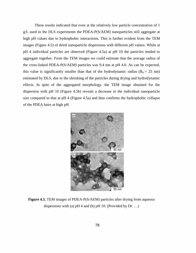
78
These results indicated that even at the relatively low particle concentration of 1
g/L used in the DLS experiments the PDEA-P(S/AEM) nanoparticles still aggregate at
high pH values due to hydrophobic interactions. This is further evident from the TEM
images (Figure 4.5) of dried nanoparticle dispersions with different pH values. While at
pH 4 individual particles are observed (Figure 4.5a) at pH 10 the particles tended to
aggregate together. From the TEM images we could estimate that the average radius of
the cross-linked PDEA-P(S/AEM) particles was 9.4 nm at pH 4.0. As can be expected,
this value is significantly smaller than that of the hydrodynamic radius (Rh ≈ 25 nm)
estimated by DLS, due to the shrinking of the particles during drying and hydrodynamic
effects. In spite of the aggregated morphology, the TEM image obtained for the
dispersion with pH 10 (Figure 4.5b) reveals a decrease in the individual nanoparticle
size compared to that at pH 4 (Figure 4.5a) and thus confirms the hydrophobic collapse
of the PDEA hairs at high pH.
Figure 4.5. TEM images of PDEA-P(S/AEM) particles after drying from aqueous
dispersions with (a) pH 4 and (b) pH 10. (Provided by Dr. …)

79
4.4 Monitoring the pH-responsive behavior at individual
particle level
In order to monitor pH dependent hydrophilic-hydrophobic transition of the
PDEA hairs of individually dispersed nanoparticles we performed FCS experiments
with highly diluted dispersions of Bodipy labeled nanoparticles. Again, the pH value
was tuned by adding HCl and NaOH to the dispersions. The concentration of PDEA-
P(S/Bodipy) under different pH conditions was always kept at 0.02 g/L, which is 50
times less than the concentration used in the DLS experiments. Typical FCS auto-
correlation curves measured at various pH values are shown in Figure 4.6a. With
increasing pH the curves shift to the shorter lag times, reflecting the decrease in particle
size and thus the faster diffusion. The experimental auto-correlation curves could be
well fitted with Equation 2.8 yielding the diffusion coefficients, and through the Stokes-
Einstein relation, the hydrodynamic radius, Rh of the hairy nanoparticles. Figure 4.6b
shows the Rh values obtained over broad pH range. The value at low pH, Rh=23 nm is
very similar to that measured by DLS (Figure 4.4b), which confirms the accuracy of the
FCS data. However, in contrast to the DLS studies, with the increase of pH, the
measured hydrodynamic radius decreases continuously down to a value Rh = 10 nm at
pH 12. These results show that at the very low concentrations assessable by FCS the
particle aggregation caused by hydrophobic interactions can be strongly diminished and
the pH-responsiveness of the PDEA hairs can be monitored on individual nanoparticle
level. Moreover, compared to the DLS result (Figure 4.4b) the FCS data shown in
Figure 4.6b reveal a less sharp transition that extends over a broad pH range. This effect
may be related to the much lower concentration at which the FCS measurements were
performed and possibly to the coexistence of PDEA hairs at different stage of the
collapse at a given overall pH value.

80
Figure 4.6. (a) Normalized, experimental FCS autocorrelation curves measured for
aqueous dispersions of Bodipy labeled nanoparticles at Cp = 0.02 g/L and different pH
values. The solid lines represent the corresponding fits with Equation 2.8. (b)
Hydrodynamic radius Rh of the nanoparticles as a function of pH. The solid line is to
guide the eye.
The results summarized in Table 4.2 clearly demonstrate that depending on the
experimental conditions different techniques may provide different values for the
nanoparticle size and this may lead to certain confusion if the experimental conditions
are not well specified. For the system considered here at low pH values (pH 4) the
PDEA shell of the nanoparticles is hydrophilic and they are well dispersed (not
aggregating) over broad concentration range. At these conditions both DLS and FCS

81
provide very similar values for the hydrodynamic radius, i.e. 25.4±3 nm and 22.8±3 nm
respectively. At high pH values (pH 10) the PDEA shell of the nanoparticles exhibits
hydrophobic collapse and the hydrodynamic radius of the individual nanoparticles
decreases to around 12±2 nm as measured by FCS at very low concentrations of 0.02
g/L. DLS could not track this effect because at the higher concentration needed for DLS
(1 g/L) the hydrophobic collapse is associated with particles aggregation and thus DLS
measures an average aggregate hydrodynamic radius of around 70 nm. On the other
hand for the TEM studies nanoparticles have to be studied in the dry state that leads to
complete shrinking of the nanoparticles and systematically lower values for their size. It
is important to emphasize at this point that depending on the experimental conditions
different techniques may provide different values for the nanoparticles size (Table 4.2),
and therefore the exact experimental conditions should be always carefully considered.
Table 4.2. Rh of hairy nanoparticles measured by DLS, FCS and TEM.
DLS FCS TEM
Concentration (g/L) 1.0 0.02 dry
Particle size at pH 4
(nm)
25.4 22.8 9.4
Particle size at pH
7.5 (nm)
40.0 15.0 -
Particle size at pH
10 (nm)
71.2 11.8 aggregation
Such experimental condition is example the concentration that is different for the
DLS and FCS studies (Table 4.2). In order to further illustrate this, I used dispersion of
hairy nanoparticle with 1.0 g/L concentration, the same concentration of DLS

82
measurement and studied it by FCS. Figure 4.7 shows the autocorrelation curves of
hairy nanoparticle in aqueous solution of pH = 5.0 and pH = 7.5. It clearly shows that at
pH = 7.5, the curve shift to long lag times indicating slower diffusion and bigger size,
which is in accordance with the DLS result, confirming that the concentration plays a
big rule on the dispersed state of hairy nanoparticles.
10-5
10-4
10-3
10-2
10-1
0.0
0.2
0.4
0.6
0.8
1.0
pH 5.0
pH 7.5
G(
)
/ s
Figure 4.7. Autocorrelation functions G(τ) for the diffusion of the hairy nanoparticle at
1 g/L. (The same concentration of DLS measurement)
Next, I studied the reversibility of the pH induced collapse on the grafted PDEA
chains. Therefore, we consecutively tuned the pH of the nanoparticle dispersion between
4.0 and 11. Figure 4.8a are the autocorrelation curves of hairy nanoparticles at pH = 4.0
and pH = 11.0. As shown in Figure 4.8b, the hydrodynamic radius of the particles
changed reversibly from 23 nm at low pH to 11 nm at high pH values. The cycle was
repeated only 3 times because the continuous addition of NaOH and HCl solutions to the
dispersion increased its total volume and thus decreased the concentration of the
nanoparticles to the edge of the FCS sensitivity.

83
Figure 4.8. (a) Autocorrelation curve of hairy nanoparticles at pH = 4.0 and pH = 11.0.
The solid lines represent the corresponding fits with Equation 2.8. (b) Hydrodynamic
radius, Rh, as a function of pH upon cycling the pH value between 4.0 and 11.0.
4.5 Comparison of the pH-responsiveness of the hairy
nanoparticles and single chains
In an attempt to compare the pH induced collapse of PDEA chains attached to
the surface of a nanoparticle and to that of freely diffusing chains, Bodipy-labeled

84
polymer (P(DEA/Bodipy)) was prepared as described in the experimental part and the
hydrodynamic radius of the individual chains was measured with FCS. The experiments
were performed in extremely diluted solutions (0.003 g/L) at various pH. Under acid
conditions, the polymer chains were well dispersed in the solution. FCS autocorrelation
curves (Figure 4.9a) could easily be recorded and the individual chain hydrodynamic
radius could be calculated (Figure 4.9b). As expected, the hydrodynamic radius
continuously decreased with the increase of pH, reflecting the hydrophobic collapse of
the chains. However, as discussed above the increase of pH leads to a strong decrease in
the fluorescent brightness of the Bodipy labels. Furthermore, the PDEA chains carry
only one dye per chain and thus their fluorescent brightness is significantly weaker than
that of the nanoparticles (with ~9 dyes per particle). Due to these reasons and possibly
some additional hydrophobic effects, e.g. chain migration to the water/air interface of
the sample chamber, we were not able to record reasonable FCS autocorrelation curves
and determine the hydrodynamic radius of individual PDEA chains at high pH values.
The data shown in Figure 4.9 indicates that when the pH increased from 2.3 to 5.1 the
hydrodynamic radius of the P(DEA/Bodipy) chains (Mn = 18000 g/mol) decreased from
2.9 nm to 2.2 nm, i.e. with 0.7 nm (hydrodynamic diameter decreased with 1.4 nm). For
comparison the hydrodynamic radius of the nanoparticles processing grafted PDEA
hairs with similar molecular weight (Mn = 15500 g/mol) decreased by 1.6 nm in the
same pH range (Figure 4.9b). While the estimated hydrodynamic radius (diameters)
should be considered only as an approximation for the real chain dimensions, the
obtained values indicate that the chains grafted to the PS nanoparticles contract in a
similar way and to similar extend compared to freely diffusing chains.

85
Figure 4.9. (a) Autocorrelation curves of PDEA hair and PDEA single chain at pH 3.0.
The solid lines represent the corresponding fits with Equation 2.8. (b) Plot of Rh as a
function of pH for PDEA hairs (0.02 g/L).and single chain solution (0.003 g/L).
4.6 Controlling the mobility of the pH-responsive particles in
nanoporous environment
Some of the most important applications of the stimuli-responsive nanoparticles
are related to the possibility to control their mobility in nanoporous media. In such

86
environment even small changes of the particle size may have a profound effect on the
mobility. With this in mind, we studied the diffusion of the PDEA-P(S/Bodipy)
nanoparticles (PDEA-P(S/Bodipy)) in a water filled silica inverse opal at various pH
values.
A silica inverse opal consists of a regular arrangement of spherical voids
surrounded by solid silica walls with interconnecting circular pores. It was chosen as a
model for well-defined nanoporous structure.[73, 74, 86, 87] The particular structure
used in this study (Figure 2.9c in chapter 2) had a void diameter of 920 nm and
interconnecting pores diameter of 240 nm. It was infiltrated with aqueous dispersion of
the PDEA-P(S/Bodipy) nanoparticles. The particles’ diffusion coefficient was measured
with FCS. Prior to the FCS measurements the structure was imaged using the reflection
mode of the confocal microscope in order to confirm the regular porosity and the
absence of defects (Figure 4.10a) at the point where the FCS measurements were
performed. Figure 4.10b shows typical FCS autocorrelation curves measured in the
inverse opal at pH = 9.0 and pH = 4.0. For comparison the autocorrelation curves
measured in free aqueous environment (without inverse opal) are also shown. It should
be noted that because the nanoparticle’s diffusion is confined in the inverse opal voids,
which have sizes similar to that of the FCS probing volume, the use of Equation 2.8 that
is derived for free 3D diffusion is not trivial. However, as Equation 2.8 represents very
well the experimentally measured autocorrelation curves (Figure 4.10b) we still used it
as a preliminary, approximate way to estimate the diffusion coefficients of the
nanoparticles in the inverse opals. The curves measured in the inverse opal are shifted to
the longer lag times, reflecting the significantly slower diffusion in the nanoporous
structure. Furthermore, the change in pH from 4.0 to 9.0 affects significantly stronger
the mobility of the nanoparticles in the inverse opal. To quantify this effect we have
fitted the autocorrelation curves with Equation 2.8 and determined the respective
diffusion coefficients of the nanoparticles. In free aqueous environment the diffusion
coefficient increased from 1.0 × 10⁻¹¹
m2/s to 2.0 × 10
-11 m
2/s when the pH was changed
from 4.0 to 9.0. The corresponding values in silica inverse opal were from 4.0 × 10⁻¹²

87
m2/s to 1.05 × 10
-11 m
2/s, respectively. Thus, the pH induced change in mobility
(diffusion coefficient) was significantly larger in the silica inverse opal, reflecting the
stronger effect of the nanoparticle size on the mobility in the porous environment.
Figure 4.10. (a) A confocal microscopy image (in reflection mode) of water infiltrated
silica inverse opal. (b) Experimental autocorrelation curves for the diffusion of the
Bodipy labeled hairy nanoparticle in the iOpal made from 1 µm PS particles (red
squares) and in free aqueous environment (green circles) at pH 9.0 (open symbols) and
pH 4.0 (solid symbols). The solid lines represent the corresponding fits with Equation
2.8.

88
Another inverse opal made from 330 nm PS nanoparticles is also used as a
model for well-defined nanoporous structure (SEM image is shown in Figure 2.9b in
chapter 2 and reflectance mode image by FCS is shown in Figure 3.1 in chapter 3).
Figure 4.11 also shows the change in pH from 4.0 to 9.0 affects significantly stronger
the mobility of the nanoparticles in the inverse opal. The autocorrelation curves were
fitted with Equation 2.8 and determined the respective diffusion coefficients of the
nanoparticles. In the smaller hole with 315 nm in diameter, the diffusion coefficient in
silica iOpal was from 3.0 × 10⁻¹²
m2/s to 7.2 × 10
-12 m
2/s from 4.0 to 9.0, respectively.
These values show that in smaller iOpal the mobility control of the tracer is more
significant than free aqueous solution.
10-5
10-4
10-3
10-2
10-1
0.0
0.2
0.4
0.6
0.8
1.0
water pH 9.0
IO330 pH 9.0
water pH 4.0
IO330 pH 4.0
G(
)
/ s
Figure 4.11. Experimental autocorrelation curves for the diffusion of the Bodipy labeled
hairy nanoparticle in the iOpal made from 330 nm nanoparticle (red squares) and in free
aqueous environment (green circles) at pH 9.0 (open symbols) and pH 4.0 (solid
symbols). The solid lines represent the corresponding fits with Equation 2.8.

89
4.7 Conclusion
I showed that due to its very high sensitivity FCS can be used to measure the
stimuli-responsiveness of individual hairy nanoparticles. Using this technique I found
that when the pH is increased, PDEA chains grafted to a small polystyrene core collapse
similarly to freely diffusing PDEA chains. The particle concentration plays an important
role on the general behavior of stimuli-responsive hairy nanoparticles. At high and
moderately low concentrations, the pH induced collapse leads to aggregation and thus
lowering of the nanoparticles mobility. At very low concentrations, however, the
hydrophobic collapse is associated with decrease of nanoparticles size and increase in
their mobility. The later effect is particularly evident and important when the
nanoparticles are dispersed in nanoporous environment.

90

91
CHAPTER 5
Summary and conclusion
Controlling the mobility of molecules, macromolecules, nanoparticles etc. in
solution and in complex, nanostructured environments is of vital importance, as
diffusion is the dominant mechanism for the transport of such species in e.g. solid
nanoporous structures, polymer solutions and gels, or in living cells. In this thesis I
described how using stimuli-responsive polymers, one can design a stimuli-responsive
system in which the mobility of molecules and nanoparticles in solution or nanoporous
environment can be controlled, and the whole process can be monitored in situ by
fluorescence correlation spectroscopy (FCS).
First, I prepared silica inverse opals (iOpal), which are well-defined, highly
ordered porous structures and with high mechanic stability. By modifying iOpal with
poly(N-isopropylacrylamide) (PNIPAM) I obtained a stimuli-responsive system with
two levels of porosity. By simply tuning the temperature below or above the lower
critical solution temperature of PNIPAM, it was possible to change the size of the pores
and thus control the mobility of small species in them. Moreover, the mobility changes
caused by the PNIPAM brushes as temperature changes were fully reversible after
several heating and cooling cycles. In this way the mobility of the small species is
controllable by just immersing them in the responsive nanoporous environment.
Second, I prepared the PS/PDEA hairy nanoparticles with pH-responsive hairs.
Owing to the high, single molecule sensitivity of FCS, colloid aggregation of hairy
nanoparticles can be avoided and the pH induced collapse of hairs can be monitored at
very low concentration, which means I can observe the hydrophobic collapse of pH-
responsive hairy nanoparticles at individual particle level. By increasing the pH of the
solution gradually, the hairs would collapse accordingly, thus the size of hairy
nanoparticle would decrease and they would show faster mobility. Furthermore, I found

92
that PDEA chains grafted to a small polystyrene core collapse similarly to freely
diffusing PDEA chains as pH in solution changes. When the nanoparticles are dispersed
in nanoporous environment, faster mobility induced by decreased nanoparticle size is
particularly evident. In this way I prepared responsive nanoparticles which show
controllable mobility in diverse environments.
In brief, I have produced stimuli-responsive systems, in which one can control
the mobility control of species in aqueous solutions and confined nanoporous
environments. Owing to the high sensitivity of FCS technique, this effect can be
monitored in situ and the mobility of the species can be traced.

93
Acknowledgement
…

94
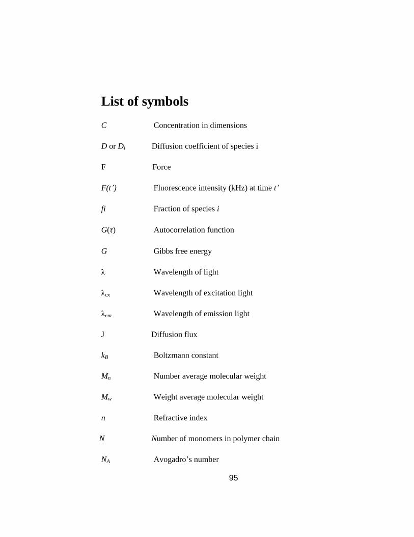
95
List of symbols
C Concentration in dimensions
D or Di Diffusion coefficient of species i
F Force
F(t’) Fluorescence intensity (kHz) at time t’
fi Fraction of species i
G(τ) Autocorrelation function
G Gibbs free energy
λ Wavelength of light
λex Wavelength of excitation light
λem Wavelength of emission light
J Diffusion flux
kB Boltzmann constant
Mn Number average molecular weight
Mw Weight average molecular weight
n Refractive index
N Number of monomers in polymer chain
NA Avogadro’s number

96
Np number of particles in the observation volume
<Δr²(t)> Mean square displacement
Rh Hydrodynamic radius
r0 Radial axis of confocal volume
S Structure of parameter (= z0/r0)
t Experimental lag time
τD Lateral diffusion time
T Temperature
T0 Ideal glass transition temperature
Tg Glass transition temperature
V Observation volume
ν Particle moving speed
z0 Vertical axis of confocal volume
η Viscosity
𝛻 Gradient operator
Δ Laplacian, the second derivative
μ Particle mobility
r Radius of particle
q Electrical charge
ɸ Weight fraction

97
List of abbreviations
ATRP Atom transfer radical polymerization
DLS dynamic light scattering
FCS Fluorescence correlation spectroscopy
GPC Gel Permeation Chromatography
NA Numerical aperture
NMR Nuclear magnetic resonance
PDEAEMA Poly(2-diethylaminoethyl methacrylate)
PNIPAM Poly (N-isopropylacrylamide)
PS Polystyrene
Qdot Quantum dot
VD Vertical deposition
THF Tetrahydrofuran

98
99
References
1. Einstein, A., Über die von der molekularkinetischen Theorie der Wärme
geforderte Bewegung von in ruhenden Flüssigkeiten suspendierten Teilchen.
Ann. Phys. , 1905. 17: p. 549–560.
2. Fick, A., Ueber Diffusion. Ann. der. Physik, 1855. 94: p. 59-86.
3. Fick, A., On liquid diffusion. Journal of Membrane Science, 1995. 100: p. 33-38.
4. Smoluchowski, M., Zur kinetischen Theorie der Brownschen
Molekularbewegung und der Suspensionen. Ann. der. Physik, 1906. 326(14): p.
756-780.
5. Stuart, M.A.C., et al., Emerging applications of stimuli-responsive polymer
materials. Nature Materials, 2010. 9(2): p. 101-113.
6. Grubbs, R.B. and Z. Sun, Shape-changing polymer assemblies. Chemical
Society Reviews, 2013. 42(17): p. 7436-7445.
7. Roy, D., W.L.A. Brooks, and B.S. Sumerlin, New directions in
thermoresponsive polymers. Chemical Society Reviews, 2013. 42(17): p. 7214-
7243.
8. Scarpa, J.S., D.D. Mueller, and I.M. Klotz, Slow hydrogen-deuterium exchange
in a non-.alpha.-helical polyamide. Journal of the American Chemical Society,
1967. 89(24): p. 6024-&.
9. Zhai, L., Stimuli-responsive polymer films. Chemical Society Reviews, 2013.
42(17): p. 7148-7160.
10. Ward, M.A. and T.K. Georgiou, Thermoresponsive Polymers for Biomedical
Applications. Polymers, 2011. 3(3): p. 1215-1242.
11. Peng, T. and Y.L. Cheng, Temperature-responsive permeability of porous
PNIPAAm-g-PE membranes. Journal of Applied Polymer Science, 1998. 70(11):
p. 2133-2142.
12. Chang, Y., et al., Tunable Bioadhesive Copolymer Hydrogels of
Thermoresponsive Poly(N-isopropyl acrylamide) Containing Zwitterionic
Polysulfobetaine. Biomacromolecules, 2010. 11(4): p. 1101-1110.
13. Haraguchi, K., K. Uyama, and H. Tanimoto, Self-healing in Nanocomposite
Hydrogels. Macromolecular Rapid Communications, 2011. 32(16): p. 1253-
1258.
14. Gibson, M.I. and R.K. O'Reilly, To aggregate, or not to aggregate?
considerations in the design and application of polymeric thermally-responsive
nanoparticles. Chemical Society Reviews, 2013. 42(17): p. 7204-7213.
15. M. Heskins, J.E.G., Solution Properties of Poly(Nisopropylacrylamide). J.
Macromol. Sci.- Chem, 1968. 2(8): p. 1441-1455.
16. Chen, G.H. and A.S. Hoffman, Graft copolymers that exhibit temperature-
induced phase transitions over a wide range of pH. Nature, 1995. 373(6509): p.
49-52.
17. Kujawa, P., et al., Impact of end-group association and main-chain hydration on
the thermosensitive properties of hydrophobically modified telechelic poly(N-
isopropylacrylamides) in water. Macromolecules, 2006. 39(1): p. 341-348.

100
18. Schmaljohann, D., Thermo- and pH-responsive polymers in drug delivery.
Advanced Drug Delivery Reviews, 2006. 58(15): p. 1655-1670.
19. Kharlampieva, E., et al., Hydrogen-bonded multilayers of thermoresponsive
polymers. Macromolecules, 2005. 38(25): p. 10523-10531.
20. Chunder, A., et al., Conformal switchable superhydrophobic/hydrophilic
surfaces for microscale flow control. Colloids and Surfaces a-Physicochemical
and Engineering Aspects, 2009. 333(1-3): p. 187-193.
21. Huber, D.L., et al., Programmed adsorption and release of proteins in a
microfluidic device. Science, 2003. 301(5631): p. 352-354.
22. Zhou, Y.M., et al., Deposition transfection technology using a DNA complex
with a thermoresponsive cationic star polymer. Journal of Controlled Release,
2007. 123(3): p. 239-246.
23. Dai, S., P. Ravi, and K.C. Tam, pH-Responsive polymers: synthesis, properties
and applications. Soft Matter, 2008. 4(3): p. 435-449.
24. Tang, Y.Q., et al., Solubilization and controlled release of a hydrophobic drug
using novel micelle-forming ABC triblock copolymers. Biomacromolecules,
2003. 4(6): p. 1636-1645.
25. Tian, W., et al., Multiresponsive Properties of Triple-Shell Architectures with
Poly(N,N-diethylaminoethyl methacrylate), Poly(N-vinylcaprolactam), and
Poly(N,N-dimethylaminoethyl methacrylate) as Building Blocks.
Macromolecular Chemistry and Physics, 2012. 213(23): p. 2450-2463.
26. Alexander, S., Adsorption of chain molecules with a polar head a scaling
description. Journal De Physique, 1977. 38(8): p. 983-987.
27. Degennes, P.G., Conformations of polymers attached to an interface
Macromolecules, 1980. 13(5): p. 1069-1075.
28. Milner, S.T., Polymer Brushes. Science, 1991. 251(4996): p. 905-914.
29. Zhou, C., M.A. Hillmyer, and T.P. Lodge, Micellization and Micelliar
Aggregation of Poly(ethylene-alt-propylene)-b-poly(ethylene oxide)-b-poly(N-
isopropylacrylamide) Triblock Terpolymers in Water. Macromolecules, 2011.
44(6): p. 1635-1641.
30. Ishida, N. and S. Biggs, Salt-induced structural behavior for poly(N-
isopropylacryamide) grafted onto solid surface observed directly by AFM and
QCM-D. Macromolecules, 2007. 40(25): p. 9045-9052.
31. Laloyaux, X., et al., Surface and Bulk Collapse Transitions of Thermo
responsive Polymer Brushes. Langmuir, 2010. 26(2): p. 838-847.
32. Bradley, C., et al., Response Characteristics of Thermoresponsive Polymers
Using Nanomechanical Cantilever Sensors. Macromolecular Chemistry and
Physics, 2009. 210(16): p. 1339-1345.
33. Hoffman, A.S., The origins and evolution of "controlled" drug delivery systems.
Journal of Controlled Release, 2008. 132(3): p. 153-163.
34. Hayashi, G., et al., Photoregulation of a peptide-RNA interaction on a gold
surface. Journal of the American Chemical Society, 2007. 129(28): p. 8678-
8679.

101
35. Tokareva, I., et al., Nanosensors based on responsive polymer brushes and gold
nanoparticle enhanced transmission surface plasmon resonance spectroscopy.
Journal of the American Chemical Society, 2004. 126(49): p. 15950-15951.
36. Urban, M.W., Intelligent polymeric coatings; Current and future advances.
Polymer Reviews, 2006. 46(4): p. 329-339.
37. Lu, Y., et al., Thermosensitive core-shell particles as carriers for Ag
nanoparticles: Modulating the catalytic activity by a phase transition in
networks. Angewandte Chemie-International Edition, 2006. 45(5): p. 813-816.
38. Oishi, M., et al., Endosomal release and intracellular delivery of anticancer
drugs using pH-sensitive PEGylated nanogels. Journal of Materials Chemistry,
2007. 17(35): p. 3720-3725.
39. Hervet, H., L. Leger, and F. Rondelez, Self-Diffusion in Polymer Solutions: A
Test for Scaling and Reptation. Physical Review Letters, 1979. 42(25): p. 1681-
1684.
40. Vaz, W.L.C., et al., Size dependence of the translational diffusion of large
integral membrane proteins in liquid-crystalline phase lipid bilayers. A study
using fluorescence recovery after photobleaching. Biochemistry, 1982. 21(22):
p. 5608-5612.
41. Callaghan, P.T. and D.N. Pinder, A pulsed field gradient NMR study of self-
diffusion in a polydisperse polymer system: dextran in water. Macromolecules,
1983. 16(6): p. 968-973.
42. Schillen, K., W. Brown, and R.M. Johnsen, Micellar Sphere-to-Rod Transition
in an Aqueous Triblock Copolymer System. A Dynamic Light Scattering Study of
Translational and Rotational Diffusion. Macromolecules, 1994. 27(17): p. 4825-
4832.
43. Jobic, H. and D.N. Theodorou, Quasi-elastic neutron scattering and molecular
dynamics simulation as complementary techniques for studying diffusion in
zeolites. Microporous and Mesoporous Materials, 2007. 102(1-3): p. 21-50.
44. Rigler, R., E.S. Elson, Fluorescence correlation spectroscopy: Theory and
Applications. Springer, 2001.
45. Papadakis, C.M., et al., Polymers in focus: fluorescence correlation
spectroscopy. Colloid and Polymer Science, 2014. 292(10): p. 2399-2411.
46. Woll, D., Fluorescence correlation spectroscopy in polymer science. Rsc
Advances, 2014. 4(5): p. 2447-2465.
47. Koynov, K. and H.J. Butt, Fluorescence correlation spectroscopy in colloid and
interface science. Current Opinion in Colloid & Interface Science, 2012. 17(6):
p. 377-387.
48. Pristinski, D., V. Kozlovskaya, and S.A. Sukhishvili, Fluorescence correlation
spectroscopy studies of diffusion of a weak polyelectrolyte in aqueous solutions.
Journal of Chemical Physics, 2005. 122(1): p. 9.
49. Jia, P.X. and J. Zhao, Single chain contraction and re-expansion of polystyrene
sulfonate: A study on its re-entrant condensation at single molecular level.
Journal of Chemical Physics, 2009. 131(23): p. 4.
50. Daniels, C.R., et al., On the pH-Responsive, Charge-Selective, Polymer-Brush-
Mediated Transport Probed by Traditional and Scanning Fluorescence

102
Correlation Spectroscopy. Journal of Physical Chemistry B, 2013. 117(16): p.
4284-4290.
51. Zhang, C.F., et al., Diffusion of Ionic Fluorescent Probes atop Polyelectrolyte
Brushes. Journal of Physical Chemistry B, 2011. 115(51): p. 15167-15173.
52. Lehmann, S., S. Seiffert, and W. Richtering, Spatially Resolved Tracer Diffusion
in Complex Responsive Hydrogels. Journal of the American Chemical Society,
2012. 134(38): p. 15963-15969.
53. Raccis, R., et al., Probing mobility and structural inhomogeneities in grafted
hydrogel films by fluorescence correlation spectroscopy. Soft Matter, 2011.
7(15): p. 7042-7053.
54. Vagias, A., et al., Dynamics in Stimuli-Responsive Poly(N-isopropylacrylamide)
Hydrogel Layers As Revealed by Fluorescence Correlation Spectroscopy.
Macromolecules, 2014. 47(15): p. 5303-5312.
55. Krichevsky, O. and G. Bonnet, Fluorescence correlation spectroscopy: the
technique and its applications. Reports on Progress in Physics, 2002. 65(2): p.
251-297.
56. Magde, D., W.W. Webb, and E. Elson, Thermodynamic Fluctuations in a
Reacting System—Measurement by Fluorescence Correlation Spectroscopy.
Physical Review Letters, 1972. 29(11): p. 705-708.
57. Magde, D., E.L. Elson, and W.W. Webb, Fluorescence correlation
spectroscopy. II. An experimental realization. Biopolymers, 1974. 13(1): p. 29-
61.
58. Eigen, M. and R. Rigler, Sorting single molecules: application to diagnostics
and evolutionary biotechnology. Proceedings of the National Academy of
Sciences of the United States of America, 1994. 91(13): p. 5740-5747.
59. Yordanov, S., Total Internal Reflection Fluorescence Cross-Correlation
Spectroscopy: theory and application for studying boundary slip phenomenon, in
Physik, Mathematik und Informatik. 2011, der Johannes Gutenberg-Universität
Mainz. p. 140.
60. Petrasek, Z. and P. Schwille, Precise measurement of diffusion coefficients using
scanning fluorescence correlation spectroscopy. Biophysical Journal, 2008.
94(4): p. 1437-1448.
61. Jablonski, A., Efficiency of anti-stokes fluorescence in dyes. Nature, 1933. 131:
p. 839-840.
62. AAT_Bioquest. 12/10/2015; Available from:
http://aatbio.com/gen4prst.pl?Cid=1082.
63. AAT_Bioquest. Alexa 647. 12/10/2015; Available from:
http://aatbio.com/gen4prst.pl?Cid=1031.
64. Loudet, A. and K. Burgess, BODIPY dyes and their derivatives: Syntheses and
spectroscopic properties. Chemical Reviews, 2007. 107(11): p. 4891-4932.
65. Thermofisher. Bodipy. 12/10/2015; Available from:
http://www.thermofisher.com/order/catalog/product/D2184.
66. Zrazhevskiy, P., M. Sena, and X.H. Gao, Designing multifunctional quantum
dots for bioimaging, detection, and drug delivery. Chemical Society Reviews,
2010. 39(11): p. 4326-4354.

103
67. Alivisatos, A.P., Semiconductor clusters, nanocrystals, and quantum dots.
Science, 1996. 271(5251): p. 933-937.
68. Semrock. Quantum dots. 12/10/2015; Available from:
http://www.semrock.com/fluorescence-imaging-with-quantum-dot-
nanocrystals.aspx.
69. Thermofisher. Quantum Dots. 12/10/2015; Available from:
https://www.thermofisher.com/de/de/home/references/molecular-probes-the-
handbook/ultrasensitive-detection-technology/qdot-nanocrystal-technology.html.
70. D'Acunzi, M., et al., Superhydrophobic surfaces by hybrid raspberry-like
particles. Faraday Discussions, 2010. 146: p. 35-48.
71. Gu, Z.Z., et al., Infiltration of colloidal crystal with nanoparticles using
capillary forces: a simple technique for the fabrication of films with an ordered
porous structure. Applied Physics a-Materials Science & Processing, 2002.
74(1): p. 127-129.
72. Li, Q., et al., Porous Networks Through Colloidal Templates, in Templates in
Chemistry Iii, P. Broekmann, K.H. Dotz, and C.A. Schalley, Editors. 2009,
Springer-Verlag Berlin: Berlin. p. 135-180.
73. Wang, J.J., et al., Preparation of multilayered trimodal colloid crystals and
binary inverse opals. Journal of the American Chemical Society, 2006. 128(49):
p. 15606-15607.
74. Wang, J., et al., Structural and optical characterization of 3D binary colloidal
crystal and inverse opal films prepared by direct co-deposition. Journal of
Materials Chemistry, 2008. 18(9): p. 981-988.
75. Jing Xie, K.N., Sayaka Ohno, Hans-Juergen Butt, Kaloian Koynov, Shin-ichi
Yusa, Fluorescence Correlation Spectroscopy Monitors the Hydrophobic
Collapse of pH-Responsive Hairy Nanoparticles at the Individual Particle Level.
Macromolecules, 2015. 48: p. 7237−7244.
76. Biophysics. 8-well chamber. 12/10/2015; Available from:
http://www.biophysics.com/uSLIDE8well.php.
77. Thermofisher. Attofluor Cell Chamber. 12/10/2015; Available from:
https://www.thermofisher.com/order/catalog/product/A7816.
78. Edmondson, S., V.L. Osborne, and W.T.S. Huck, Polymer brushes via surface-
initiated polymerizations. Chemical Society Reviews, 2004. 33(1): p. 14-22.
79. Barbey, R., et al., Polymer Brushes via Surface-Initiated Controlled Radical
Polymerization: Synthesis, Characterization, Properties, and Applications.
Chemical Reviews, 2009. 109(11): p. 5437-5527.
80. Kato, M., et al., Polymerization of Methyl Methacrylate with the Carbon
Tetrachloride/Dichlorotris- (triphenylphosphine)ruthenium(II)/Methylaluminum
Bis(2,6-di-tert-butylphenoxide) Initiating System: Possibility of Living Radical
Polymerization. Macromolecules, 1995. 28(5): p. 1721-1723.
81. Wang, J.S. and K. Matyjaszewski, Controlled/" living" radical polymerization.
Atom transfer radical polymerization in the presence of transition-metal
complexes. Journal of the American Chemical Society, 1995. 117(20): p. 5614-
5615.

104
82. Wang, J.S. and K. Matyjaszewski, Controlled/"Living" Radical Polymerization.
Halogen Atom Transfer Radical Polymerization Promoted by a Cu(I)/Cu(II)
Redox Process. Macromolecules, 1995. 28(23): p. 7901-7910.
83. Matyjaszewski, K., Atom Transfer Radical Polymerization (ATRP): Current
Status and Future Perspectives. Macromolecules, 2012. 45(10): p. 4015-4039.
84. Matyjaszewski, K. and J.H. Xia, Atom transfer radical polymerization. Chemical
Reviews, 2001. 101(9): p. 2921-2990.
85. Pyun, J., T. Kowalewski, and K. Matyjaszewski, Synthesis of polymer brushes
using atom transfer radical polymerization. Macromolecular Rapid
Communications, 2003. 24(18): p. 1043-1059.
86. Cherdhirankorn, T., et al., Tracer Diffusion in Silica Inverse Opals. Langmuir,
2010. 26(12): p. 10141-10146.
87. Raccis, R., et al., Confined Diffusion in Periodic Porous Nanostructures. Acs
Nano, 2011. 5(6): p. 4607-4616.
88. Nykypanchuk, D., H.H. Strey, and D.A. Hoagland, Brownian motion of DNA
confined within a two-dimensional array. Science, 2002. 297(5583): p. 987-990.
89. You, Y.Z., et al., Temperature-controlled uptake and release in PNIPAM-
modified porous silica nanoparticles. Chem. Mater., 2008. 20(10): p. 3354-3359.
90. Vasani, R.B., et al., Stimulus-Responsiveness and Drug Release from Porous
Silicon Films ATRP-Grafted with Poly(N-isopropylacrylamide). Langmuir,
2011. 27(12): p. 7843-7853.
91. Elson, E., R. Rigler, and E.S. Elson, Fluorescence correlation spectroscopy -
Theory and applications - Introduction, in Fluorescence Correlation
Spectroscopy: Theory and Applications. 2001, Springer-Verlag Berlin: Berlin. p.
1-6.
92. Kim, S.A., K.G. Heinze, and P. Schwille, Fluorescence correlation spectroscopy
in living cells. Nature Methods, 2007. 4(11): p. 963-973.
93. Zettl, H., et al., Fluorescence correlation spectroscopy of single dye-labeled
polymers in organic solvents. Macromolecules, 2004. 37(5): p. 1917-1920.
94. Bonne, T.B., et al., Aggregation behavior of amphiphilic poly(2-alkyl-2-
oxazoline) diblock copolymers in aqueous solution studied by fluorescence
correlation spectroscopy. Colloid. Polym. Sci., 2004. 282(8): p. 833-843.
95. Michelman-Ribeiro, A., et al., Probe diffusion in aqueous poly(vinyl alcohol)
solutions studied by fluorescence correlation spectroscopy. Biomacromolecules,
2007. 8(5): p. 1595-1600.
96. Zettl, H., et al., Direct observation of single molecule mobility in semidilute
polymer solutions. Physical Review E, 2007. 75(6): p. 6.
97. Gianneli, M., et al., Local and global dynamics of transient polymer networks
and swollen gels anchored on solid surfaces. Journal of Physical Chemistry C,
2007. 111(35): p. 13205-13211.
98. Woell, D., et al., Radical polymerization tracked by single molecule
spectroscopy. Angewandte Chemie-International Edition, 2008. 47(4): p. 783-
787.

105
99. Grabowski, C.A. and A. Mukhopadhyay, Diffusion of polystyrene chains and
fluorescent dye molecules in semidilute and concentrated polymer solutions.
Macromolecules, 2008. 41(16): p. 6191-6194.
100. Cherdhirankorn, T., et al., Fluorescence Correlation Spectroscopy Study of
Molecular Probe Diffusion in Polymer Melts. Macromolecules, 2009. 42(13): p.
4858-4866.
101. Modesti, G., et al., Diffusion in Model Networks as Studied by NMR and
Fluorescence Correlation Spectroscopy. Macromolecules, 2009. 42(13): p.
4681-4689.
102. Dorfschmid, M., et al., Translational and Rotational Diffusion during Radical
Bulk Polymerization: A Comparative Investigation by Full Correlation
Fluorescence Correlation Spectroscopy (fcFCS). Macromolecules, 2010. 43(14):
p. 6174-6179.
103. Wang, F., et al., Conformational Transition of Poly(N-isopropylacrylamide)
Single Chains in Its Cononsolvency Process: A Study by Fluorescence
Correlation Spectroscopy and Scaling Analysis. Macromolecules, 2012. 45(22):
p. 9196-9204.
104. Doroshenko, M., et al., Monitoring the Dynamics of Phase Separation in a
Polymer Blend by Confocal Imaging and Fluorescence Correlation
Spectroscopy. Macromolecular Rapid Communications, 2012. 33(18): p. 1568-
1573.
105. Wang, D.P., et al., Probing Diffusion of Single Nanoparticles at Water-Oil
Interfaces. Small, 2011. 7(24): p. 3502-3507.
106. Mahurin, S.M., S. Dai, and M.D. Barnes, Probing the diffusion of a dilute dye
solution in mesoporous glass with fluorescence correlation spectroscopy. J.
Phys. Chem. B, 2003. 107(48): p. 13336-13340.
107. McCain, K.S., P. Schluesche, and J.M. Harris, Poly(amidoamine) dendrimers as
nanoscale diffusion probes in sol-gel films investigated by total internal
reflection fluorescence spectroscopy. Anal. Chem., 2004. 76(4): p. 939-946.
108. Lytle, J.C. and A. Stein, Recent progress in syntheses and applications of inverse
opals and related macroporous materials prepared by colloidal crystal
templating. ChemInform, 2010. 41(28).
109. Velev, O.D. and A.M. Lenhoff, Colloidal crystals as templates for porous
materials. Current opinion in colloid & interface science, 2000. 5(1): p. 56-63.
110. Ramakrishnan, A., R. Dhamodharan, and J. Ruhe, Controlled growth of PMMA
brushes on silicon surfaces at room temperature. Macromol. Rapid Commun.,
2002. 23(10-11): p. 612-616.
111. Brunger, A.T., Free R value: a novel statistical quantity for assessing the
accuracy of crystal structures. Nature, 1992. 355(6359): p. 472-475.
112. Enderlein, J., et al., Art and artefacts of fluorescence correlation spectroscopy.
Current Pharmaceutical Biotechnology, 2004. 5(2): p. 155-161.
113. Mills, R., Self-Diffusion in Normal and Heavy Water in the Range 1–45
Degrees. Journal of Physical Chemistry, 1973. 77(5): p. 685-688.
114. Holz, M., S.R. Heil, and A. Sacco, Temperature-dependent self-diffusion
coefficients of water and six selected molecular liquids for calibration in

106
accurate H-1 NMR PFG measurements. Physical Chemistry Chemical Physics,
2000. 2(20): p. 4740-4742.
115. Vagias, A., et al., Complex Tracer Diffusion Dynamics in Polymer Solutions.
Phys. Rev. Lett., 2013. 111(8): p. 5.
116. Jochum, F.D., et al., Thermo- and Light-Responsive Polymers Containing
Photoswitchable Azobenzene End Groups. Macromolecules, 2009. 42(20): p.
7854-7862.
117. Zhou, F., et al., Polyelectrolyte brush amplified electroactuation of
microcantilevers. Nano Letters, 2008. 8(2): p. 725-730.
118. Magnusson, J.P., et al., Ion-sensitive "isothermal" responsive polymers prepared
in water. Journal of the American Chemical Society, 2008. 130(33): p. 10852-
10853.
119. Andreeva, D.V., et al., Self-healing anticorrosion coatings based on pH-sensitive
polyelectrolyte/inhibitor sandwichlike nanostructures. Advanced Materials,
2008. 20(14): p. 2789-2794.
120. Cavallaro, A., S. Taheri, and K. Vasilev, Responsive and "smart" antibacterial
surfaces: Common approaches and new developments (Review). Biointerphases,
2014. 9(2): p. 10.
121. Shen, Z., et al., Thermosensitive polymer-conjugated albumin nanospheres as
thermal targeting anti-cancer drug carrier. European Journal of Pharmaceutical
Sciences, 2008. 35(4): p. 271-282.
122. Mei, Y., et al., Catalytic activity of palladium nanoparticles encapsulated in
spherical polyelectrolyte brushes and core-shell microgels. Chemistry of
Materials, 2007. 19(5): p. 1062-1069.
123. Amalvy, J.I., et al., Use of sterically-stabilised polystyrene latex particles as a
pH-responsive particulate emulsifier to prepare surfactant-free oil-in-water
emulsions. Chemical Communications, 2003(15): p. 1826-1827.
124. Dupin, D., S.P. Armes, and S. Fujii, Stimulus-Responsive Liquid Marbles.
Journal of the American Chemical Society, 2009. 131(15): p. 5386-5387.
125. Kotsuchibashi, Y., et al., Construction of 'smart' surfaces with polymer
functionalized silica nanoparticles. Polymer Chemistry, 2013. 4(4): p. 1038-
1047.
126. Fujii, S., et al., Surface characterization of nanoparticles carrying pH-
responsive polymer hair. Polymer, 2010. 51(26): p. 6240-6247.
127. Li, D.J., et al., Thermosensitive hairy hybrid nanoparticles synthesized by
surface-initiated atom transfer radical polymerization. Langmuir, 2006. 22(7):
p. 3344-3351.
128. Yu, F.Q., X.D. Tang, and M.S. Pei, Facile synthesis of PDMAEMA-coated
hollow mesoporous silica nanoparticles and their pH-responsive controlled
release. Microporous and Mesoporous Materials, 2013. 173: p. 64-69.
129. Chen, M.Q., et al., Thermosensitive behavior of poly(N-isopropylacrylamide)
grafted polystyrene nanoparticles. Polymer Journal, 2003. 35(12): p. 901-910.
130. Adelsberger, J., et al., The collapse transition and the segmental dynamics in
concentrated micellar solutions of P(S-b-NIPAM) diblock copolymers. Colloid
and Polymer Science, 2011. 289(5-6): p. 711-720.

107
131. Kayitmazer, A.B., et al., Protein-polyelectrolyte interactions. Soft Matter, 2013.
9(9): p. 2553-2583.
132. Koynov, K. and H.J. Butt, Particle and Tracer Diffusion in Complex Liquids. 4th
International Symposium on Slow Dynamics in Complex Systems: Keep Going
Tohoku, 2013. 1518: p. 357-364.

108

109
Curriculum Vitae
Jing Xie
Master of Science
29. April 1988 in China
Richard Schirrmann Str 14
55122 Mainz
+49 176/82913698
EDUCATION
10/2012- present Max Planck Institute for polymer research Mainz, Germany
Degree to be obtained: Doctor in natural science
09/2009-07/2012 Jilin University Changchun, China
Master’s degree in polymer chemistry and physics
09/2005-07/2009 Jilin University Changchun, China
Bachelor’s degree in polymer materials and engineering

110
CONFERENCE
2th Fluorescence Correlation Spectroscopy in Polymer Science (FCS Workshop),
24th-25th, September, 2015. Aachen, Germany
10th Zsigmondy Colloquium, 07th – 08th, April, 2014. Konstanz, Germany.
15th Conference of the International Association of Colloid and Interface Scientists
(IACIS), 24th-29th, May, 2014. Mainz, Germany
PUBLISHED PAPERS
Jing Xie, Mikheil Doroshenko, Ulrich Jonas, Hans-Jürgen Butt, Kaloian Koynov;
Temperature-Controlled Diffusion in PNIPAM-Modified Silica Inverse Opals. ACS
Macro Lett. 2016, 5, 190−194.
Jing Xie, Keita Nakai, Sayaka Ohno, Hans-Juergen Butt, Kaloian Koynov, Shin-ichi
Yusa; Fluorescence Correlation Spectroscopy Monitors the Hydrophobic Collapse of
pH-Responsive Hairy Nanoparticles at the Individual Particle Level.
Macromolecules, 2015, 48, 7237−7244.
Frank Schellenberger, Jing Xie, Noemí Encinas, Alexandre Hardy, Markus Klapper,
Periklis Papadopoulos, Hans-Juergen Butt, Doris Vollmer; Direct observation of
drops on slippery lubricant-infused surfaces. Soft Matter, 2015, 11, 7617-7626.
Alexander Birke, David Huesmann, Annette Kelsch, Martin Weilbacher, Jing Xie,
Matthias Bros, Tobias Bopp, Christian Becker, Katharina Landfester, Matthias Barz;
Polypeptoid-block-polypeptide Copolymers: Synthesis, Characterization, and
Application of Amphiphilic Block Copolypept(o)ides in Drug Formulations and
Miniemulsion Techniques. Biomacromolecules 2014, 15, 548-557.