Embed Size (px)
Citation preview
Int. J. of Computers, Communications & Control, ISSN 1841-9836, E-ISSN 1841-9844
Vol. VII (2012), No. 1 (March), pp. 20-38
Controlling the Double Rotary Inverted Pendulum with MultipleFeedback Delays
V. Casanova, J. Salt, R. Piza, A. Cuenca
V. Casanova, J. Salt, R. Piza, A. Cuenca
Departamento de Ingeniería de Sistemas y AutomáticaInstituto Universitario de Automática e Informática IndustrialUniversitat Politécnica de ValenciaCamino de Vera s/n 46022 Valencia (Spain)E-mail: {vcasanov, julian, rpiza, acuenca}@isa.upv.es
Abstract:
The aim of this work is the development and implementation of a controlstructure for the double rotary inverted pendulum, suitable to be used in aNetworked Control System environment. Delays are quite common in thiskind of systems and, when controlling multivariable plants, it is possible thatdifferent delays are applied to the multiple inputs and outputs of them. A con-trol structure that allows compensating individually each one of the multipleloop delays would be useful when one of these delays changes. Inverted pendu-lums are quite sensitive to delays and for this reason are appropriated plantsto be used in these conditions. The control structure is developed modifyingthe control in no-delay conditions with a generalized predictor able to dealwith unstable and non-minimum plants as the chosen one is. The proposedstructure has been simulated and implemented to control a real double rotaryinverted pendulum.Keywords:Control applications, delay compensation, distributed control,multi-loop control, multi-variable feedback control, transport delay.
1 Introduction
The main goal of this paper is to propose a control structure that deals with multivariableplants when different delays are applied to the feedback signals. Consider the scenario in figure1. A multivariable (MIMO) plant is going to be controlled by a MIMO controller. The plantoutputs are feedback into the controller and the control actions are calculated by it, followingsome predesigned control law. These actions are applied to the plant. If the communication linksbetween controller and plant is ideal, no delays are present. When a real link is used at leastone sample time delay must be considered in each communication link. The influence of thesedelays must be removed to reach the desired behavior: the one in ideal (no-delay) conditions.
In the proposed scenario sensors and actuators (i.e. AD and DA conversions) are supposedto be separated by long distances among them and from the controller. The communicationfollows different paths for output signals and control actions, suffering different transport delays.The controller used in ideal conditions must be modified to compensate these delays. This isa common situation in networked control systems (NCS) when a shared medium is used tocommunicate a number of sensors and actuators with the main control. The longer the distanceis, the greater the delay must be removed. The delay compensator becomes a MIMO structureto deal with the delay in each pair action/signal.
In wide-area NCS it is usual to have a great number of AD and DA conversions involvedin the same control structure. The communication is performed through a shared mediuminstead of using point-to-point links. This allows to reduce costs (wiring, maintenance...) and
Copyright c© 2006-2012 by CCC Publications

Controlling the Double Rotary Inverted Pendulum with MultipleFeedback Delays 21
PLA
NT
D/
AA
/D
A/
DD
/A
CO
NTR
OLLER
CO
NT
RO
LO
UTP
UT
……
d a1
dan
ds1
dsm
Figure 1: Problem scenario
to increase flexibility of the control system. The main drawbacks are the delay uncertainty andthe bandwidth limitation. If there are different distances between sensors/actuators and thecontroller and/or the priority of the devices attached to the network is different, multiple delayscan arise in the control structure.
In the most general case different number of sample time delays are applied to each one ofthe signals towards the actuators (δan being n the nth control action) and to the signals from thesensors (δsm being m the mth measured variable). The control structure becomes a collection ofnxm loops each one of them includes a δan+δsm sample time delay, from the point of view ofthe controller (loop delay). This is the delay to be compensated in the controller of each one ofthese loops in the control structure. By removing the influence of the delays, the ideal behavioris intended to be reached. The goal of this work is to use the same controller, designed withoutconsidering the delays, to deal with the problem when they are present.
The presence of multiple delays in a NCS environment has been considered in many descrip-tions of this kind of systems ( [1], [2], [3], [4], [5], [6], [7]) and several previous works have dealtwith this problem. In [8] and [9] there is a description of the problem of multiple delays in NCSwhen they are smaller than one sampling period. In [10], [11] and [12] a NCS with multipledistributed delays is modeled and an optimal control is proposed. [13] proposes a model of anNCS with multiple successive delay components in the state. [14] deals with the problem of ob-servability and optimal control in these control systems. [15] analyses the maximum allowabledelay bound in control loops with network induced delays. [16] considers the problem of multipledelays in NCS from the point of view of fault diagnosis. Some works ( [17], [18]) have consideredthe problem as a multivariable control design in which multiple input-output delays are includedin the plant model. [19] uses an observer to provide state information, comparing the systembehaviour with the Smith predictor.
The proposed solution is going to be applied to a classical control problem: the double rotary

22 V. Casanova, J. Salt, R. Piza, A. Cuenca
inverted pendulum (also known as double Furuta pendulum, see figure 2). This is a classicaltextbook example of non-linear, non-minimum phase plant. The plant to be controlled has oneinput (the control action to the motor) and three outputs (the angular position of the motorshaft, the angular position of the first rod of the inverted pendulum and the angular positionof the second rod). The goal of this control problem is to keep the pendulum angles as close tozero as possible, avoiding disturbances and to follow a certain reference with the shaft angle. So,four signals are involved between control and plant and four different time delays are going tobe considered. As it is well known, this plant is quite sensitive to delays between controller andplant becoming unstable even with small delays. This sensitivity makes the Furuta pendulumquite appropriated to the proposed environment. The controller used in ideal conditions (i.e.no delays) must be properly modified to remove the delay influence in the feedback loop. Inaddition, the plant is an unstable and non-minimum phase one which makes more difficult thedelay compensation. The single and double inverted pendulums have been widely used as atest-bed for different control strategies ( [20], [21], [22]).
Figure 2: The double rotary inverted pendulum
The paper begins with a description of the plant to be controlled (section 2), followed by thecontroller used in ideal conditions (section 3). In section 4 the controller is modified to removethe influence of the delays, considering different control-plant delays for each one of the signalsinvolved. Simulated results are presented in these sections to compare the behavior in idealconditions, the nearly-unstable behavior when delays are included and the behavior when delayinfluence is removed from the loops. Results from a real plant are presented in section 5 showinghow the proposed structure works when real disturbances and noise are present in the system.Finally, in section 6 conclusions and future work are presented.
2 Double Rotary Inverted Pendulum Model
The plant that has been chosen to implement the proposed control structure is the doublerotary inverted pendulum (double Furuta pendulum) due to its sensitivity to feedback delays.The theoretical model of this plant is described in this section and it is particularized to model

Controlling the Double Rotary Inverted Pendulum with MultipleFeedback Delays 23
a real one, the double rotary inverted pendulum developed by Quanser Consulting Inc. (shownin figure 2 in its upwards position).
The equations describing the behavior of the double inverted pendulum can be derived, usingthe Euler-Lagrange method. A complete development of this model can be found in [23] and [24].By applying the Euler-Lagrange equation to the Lagrangian (i.e. the difference between kineticand potential energy) the development of the mathematical model is greatly simplified. Figure3 shows a schematic representation (top and front view) of the plant. The variables consideredin the model are:
• θ, θ, θ: Angular position, velocity and acceleration of the motor shaft, around the verticalaxis.
• α, α, α: Angular position, velocity and acceleration of the first rod, around the motor shaftaxis.
• γ, γ, γ: Angular position, velocity and acceleration of the second rod, around the motorshaft axis.
• τ : Torque applied to the motor shaft.
• u: Control action applied to the DC motor (voltage).
Figure 3: Significant variables.
First, the torque applied by the motor must be related with the angular positions. Thethree equations defining the non-linear dynamics of the mechanical part of the pendulum can beexpressed as follows:

24 V. Casanova, J. Salt, R. Piza, A. Cuenca
τ(t) = [J1L2
1(m2 +m3)]θ(t)− [L1(m2l2 +m3L2) cosα(t)]α(t) + [m3l3L1 cos γ(t)]γ(t) + (1)
+b1θ(t) + [L1(m2l2 +m3L2) sinα(t)]α(t)2 + [m3l3L1 sin γ(t)]γ(t)
2
0 = −[L1(m2l2 +m3L2) cosα(t)]θ(t) + [J2 +m2l2
2 +m3L2
2]α(t) + (2)
+[m3l3L2 cos (γ(t)− α(t))]γ(t) + b2α(t)−
−[m3l3L2 sin (γ(t)− α(t))]γ(t)2 − [g(m2l2 +m3L2) sinα(t)]
0 = −[m3l3L1 cos γ(t)]θ(t) + [m3l3L2 cos (γ(t)− α(t)]α(t) + [J3 +m3l2
3]γ(t) + (3)
+[m3l3L2 sin (γ(t)− α(t))]α(t)2 + b3γ(t)− [gm3l3 sin γ(t)]
The parameters (whose values are provided by the manufacturer) in these equations are thelengths, masses, moments of inertia and friction coefficients of the elements in the pendulum.
• J1: Moment of inertia around the center of rotation of the motor arm.
• J2: Moment of inertia around the center of rotation of the first rod of the pendulum.
• J3: Moment of inertia around the center of of the second rod of the pendulum.
• L1: Length of the motor arm.
• L2: Length of the first rod of the pendulum.
• l2: Length between the centers of rotation and gravity of the first rod of the pendulum.
• l3: Length between the centers of rotation and gravity of the second rod of the pendulum.
• m2: Mass of the first rod of the pendulum.
• m3: Mass of the second rod of the pendulum.
• b1: Viscous friction in the joint of the motor arm.
• b2: Viscous friction in the joint of the first rod of the pendulum.
• b3: Viscous friction in the joint of the second rod of the pendulum.
• g: Acceleration of the gravity.
The non-linear model must be linearized to reach a MIMO linear model to be used in thedesign of the linear controller. The setting point for the linearization will be around α = 0 andγ = 0, , corresponding this values to the upwards position, in which the pendulum is desired toremain stable. The signal derivatives must be zero at the settling point to keep the pendulumstable. In these conditions, the three linear (linearized) equations are:
τ(t) = [J1L2
1(m2 +m3)]θ(t)− [L1(m2l2 +m3L2)α(t) + [m3l3L1]γ(t) + b1θ(t) (4)
0 = −[L1(m2l2 +m3L2)]θ(t) + [J2 +m2l2
2 +m3L2
2]α(t) + [m3l3L2]γ(t) + (5)
+b2α(t)− [g(m2l2 +m3L2)α(t)]
0 = −[m3l3L1]θ(t) + [m3l3L2]α(t) + [J3 +m3l2
3]γ(t) + b3γ(t)− [gm3l3]γ(t)] (6)
To implement the controller the input must be the voltage applied to the motor that movesthe arm that carries the pendulum rods. The relationship between the voltage applied and thetorque can be stated from the typical DC motor:

Controlling the Double Rotary Inverted Pendulum with MultipleFeedback Delays 25
τ(t) =ηgηmKgKt
Rm(u(t)−KgKmθ(t)) (7)
The mechanical parameters in this fourth equation are:
• ηg: Gearbox efficiency.
• ηm: Motor efficiency.
• Kg: Total gear ratio.
• Kt: Motor torque constant.
• Km: Motor back-EMF constant.
• Rm: Motor armature resistance.
Solving the system of four equations, the linear continuous state-space model of the plant tobe controlled can be obtained. The model must have the motor voltage as input signal and thethree angular positions as output signals. The three angular velocities are not included as outputsbecause they are not going to be measured in the real plant. The development is omitted herefor space reasons. As the goal is to control a real pendulum, the model has to be particularizedwith the real parameters (dimensions, masses, inertias, frictions, motor constants...). Theseparameters have been provided by the manufacturer. This information can be reached from theQuanser documentation [25].
As the control is going to be designed and implemented in discrete time, the continuousmodel must be discretized. The sample time is going to be 10 ms, small enough to control theplant and large enough to become unstable with a couple of sample time delays.
This model is the one to be used when designing, first, the controller in ideal conditionsand, after that, the predictor to remove the influence of the loop delays. The behavior, with andwithout the delays, must be similar in both, simulated and real systems. The delay compensationis going to be different (because the delays are different) for the three controlled variables. TheMIMO system can be divided into three SISO systems one for each of the output signals, (θ, αand γ as described before):
Gθ(z) =θ(s)
U(s)=
0.0015763(z + 0.9446)(z − 0.9432)(z − 0.8953)(z − 1.061)(z − 1.145)
(z − 1)(z − 0.9716)(z − 0.9077)(z − 1.084)(z − 1.18)(z − 0.7665)(8)
Gα(z) =α(s)
U(s)=
0.0018286(z + 0.9477)(z − 0.912)(z − 1)(z − 1.114)
(z − 0.7665)(z − 0.9077)(z − 0.9716)(z − 1.084)(z − 1.18)(9)
Gγ(z) =γ(s)
U(s)=
−0.0019976(z + 0.9538)(z − 0.9968)(z − 1)2
(z − 0.7665)(z − 0.9077)(z − 0.9716)(z − 1.084)(z − 1.18)(10)
As can be seen these transfer functions describe the dynamical behaviour of unstable andnon-minimum phase systems. The MIMO model will be used in the following section to designthe controller in ideal conditions. The three SISO models will be used in section 4 to design thepredictors for delay compensation purposes.

26 V. Casanova, J. Salt, R. Piza, A. Cuenca
3 Control Structure in No Delay Conditions
To reach the desired behavior, a Linear-Quadratic Regulator (LQR) controller is going to beused control the plant in absebtia of delays. The controller must keep the angles of the two rodsas close to zero as possible (unstable equilibrium upwards position), canceling the unavoidabledisturbances. In addition the system must follow a certain reference for the motor shaft angle.The control structure is not robust enough to cope with delays, becoming unstable, even thoughthey are very small. This ideal control will be appropriately modified to remove loop delays inthe following section. In order to improve the steady-state error of the shaft position and therobustness of the controller, the six-state model is increased including an integration term. Withthis term the motor shaft can follow step references with zero error, even with the small deadzone present in the real plant. The integral of θ(t) will be computed in the controller from themeasured angle. This augmented state is now:
X =(
θ(t) α(t) γ(t) θ(t) α(t) γ(t)∫
θ(t)dt)T
(11)
The six-state MIMO model obtained in the previous section is modified, including this newstate:
X = AX +Bu −→˙X =
(
A 0
0 0
)
X +
(
B
0
)
u (12)
Using Matlab lqr command, the seven feedback control gains for the seven states from theaugmented plant model are:
K =(
1.2824 −42.4077 −101.7583 1.8735 −11.8712 −11.5716 0.3162)
(13)
Although is not included in the model and, so, not considered when designing the controller,the real control action saturated ±10 volts. This saturation has been included in the simulationmodel. However, in ideal conditions and when the delay is compensated, the control actionalways remains in this range and the saturation can be ignored.
This controller needs the seven states as inputs to generate the control action to be appliedto the plant. In the real plant only the first three of them will be available, by means of sensorsmeasuring the angular positions. There will not be sensors to measure the other states (angularvelocities and integral error). These states are going to be computed in the control structureusing a filtered discrete derivative and a discrete integrator. So, the controller becomes a threeinputs-one output discrete system to be implemented in the control device.
As it has been described in the introduction, the three inputs of the controller are arrivingthrough different paths and different delays are applied to them. To compensate the delaysindependently it will be useful to decompose the controller into three sub-controllers, each one ofthem concerned for one of the three measured angles. The transfer functions of these individualcontrollers are as follows:
Cθ(z) =Uθ(z)
θ(z)= K(1) +K(4)Drv(z) +K(7)Int(z) = K(1) +K(4)
50z − 50
z − 0.6065+K(7)
0.01
z − 1(14)
Cα(z) =Uα(z)
α(z)= K(2) +K(5)Drv(z) = K(2) +K(5)
50z − 50
z − 0.6065(15)
Cγ(z) =Uγ(z)
γ(z)= K(3) +K(6)Drv(z) = K(3) +K(6)
50z − 50
z − 0.6065(16)

Controlling the Double Rotary Inverted Pendulum with MultipleFeedback Delays 27
Using Drv(z) and Int(z) as discrete derivator and integrator respectively, all the states canbe considered measurable. The control structure with these three sub-controllers is shown infigure 4.
Figure 4: Control structure without delay compensation.
The inner loop tries to keep γ angle as close to zero as possible, avoiding disturbances. Themiddle loop does the same with α angle. The combination of these two loops keep the pendulumin the upwards position as desired. The outer loop tries to follow the desired reference with θ
angle and drives the integral of the error to zero. As the three plant-to-control signals and thecontrol-to-plant signal are separated, different delays will be applied to the four communicationlinks to study its influence in the system performance. With the described control structure,three sub-control actions are generated and the addition of them is the control action to be sentand then applied to the plant.
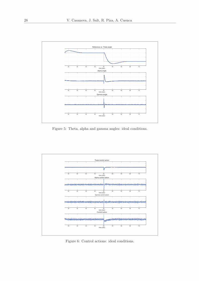
Closing the loop with the model from the previous section and the gain matrix from the LQR,the simulated results are shown in figures 5 and 6. A ±45 degrees step reference has been appliedto be tracked by the shaft angle (θ) and a small random noise has been added to the measuredpendulum angles (α and γ). No loop delay is present. Figure 5 depicts the output variables(θ, α and γ angles in degrees). As can be seen, the reference is followed properly (with zerosteady-state error) by the shaft angle and the pendulum angles are kept close to zero, despitethe noise and the changes in the main reference. Figure 6 shows the control actions of the threesub-controllers and the addition, which is the final control action to be applied to the plant. Notethat α and γ control actions are clearly influenced by the noise, added to the measured angles.
4 Control Structure with Delay Compensation
Delays in the communication between controller and plant are a well-known source of insta-bility. This is critical when controlling processes as unstable as the Furuta pendulum is. Theinfluence of the delay in the control loop must be removed to assure that the system remainsstable. Figure 7 shows the behavior of the three controlled angles when a single sample timedelay is included in the control action (with ±10 volts saturation in the control action as inthe real plant). Another sample time delay in one of the feedback signals makes the systemcompletely unstable. The sensitivity of the plant to loop delays makes this plant the ideal onefor the work in this paper. The proposal is to modify the original delay-free controller to handlewith delays even when they are different in the signals transmitted to and from the plant.
28 V. Casanova, J. Salt, R. Piza, A. Cuenca
30 35 40 45 50 55 60 65 70
Reference vs. Theta angle
time (sec)
30 35 40 45 50 55 60 65 70
Alpha angle
time (sec)
30 35 40 45 50 55 60 65 70
Gamma angle
time (sec)
Figure 5: Theta, alpha and gamma angles: ideal conditions.
30 35 40 45 50 55 60 65 70
Theta control action
time (sec)
30 35 40 45 50 55 60 65 70
Alpha control action
time (sec)
30 35 40 45 50 55 60 65 70
Gamma control action
time (sec)
30 35 40 45 50 55 60 65 70
Control action
time (sec)
Figure 6: Control actions: ideal conditions.

Controlling the Double Rotary Inverted Pendulum with MultipleFeedback Delays 29
26 28 30 32 34 36 38 40 42 44
Reference vs. Theta angle
time (sec)
26 28 30 32 34 36 38 40 42 44
Alpha angle
time (sec)
26 28 30 32 34 36 38 40 42 44
Gamma angle
time (sec)
Figure 7: Theta, alpha and gamma angles: delayed.
Smith predictor has been traditionally used to overcome delays for stable plants withoutintegral behavior. Several modifications ( [26], [27], [28]) of the original idea have been proposedto be used for multivariable plants, with different input-output delays. The limitation is thatthey usually cannot be used with non-minimum phase, unstable plants with integral behavior.The classical Smith predictor has been modified ( [29], [30], [31]) to deal with unstable plants.If all the controlled variables (i.e. all the loops in the control system) have the same delay, oneof these modified predictors could be used.
The plant to be controlled in this paper is an unstable and non-minimum MIMO (one inputand three outputs) plant but it can be easily decomposed into three SISO plants. In addition,in the scenario considered in this work, each one of the SISO plants is influenced by a differentloop delay to be compensated. Parameter δu is the number of sample time delays for the controlaction (controller-to-plant signal). Parameters δθ, δα and δγ are the delays for the shaft andpendulum angles (plant-to-controller signals). The most general case is given when the fourdelays are different, as shown in figure 4, there are three loops in the systems. The loop delay(from the output to the input of the controller) for each one of the loops is given by the additionof the control action delay and the corresponding output signal delay. These are the delays to becompensated in each one of the sub-controller. Only constant and integer multiple of the sampletime delays are considered in this work but the idea can be extended to fractional and variabledelays.
In [32] and [33] a delay compensation is proposed, suitable to be used with unstable and non-minimum phase SISO plants. The predictor proposed and described in these references (Gener-alized predictor, GP, figure 8) is stable for unstable/stable, minimum/non-minimum plants.
The inputs of the GP are the plant input (control action) and output (controlled variable).The output of the GP is the predicted signal. Depending on the quality of the plant modelused to design the predictor, the predicted signal will be equal to the controlled variable withoutthe delay. It is the same behavior than with the classical Smith predictor but, in this case,it can be used with the transfer functions of the inverted pendulum. From the (unstable non-minimum phase) transfer function and the known loop delay the GP can be designed. This GP
30 V. Casanova, J. Salt, R. Piza, A. Cuenca
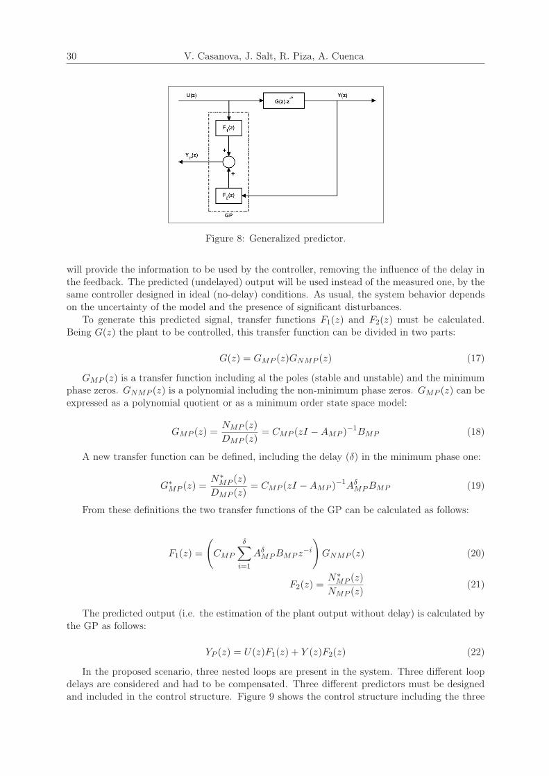
Figure 8: Generalized predictor.
will provide the information to be used by the controller, removing the influence of the delay inthe feedback. The predicted (undelayed) output will be used instead of the measured one, by thesame controller designed in ideal (no-delay) conditions. As usual, the system behavior dependson the uncertainty of the model and the presence of significant disturbances.
To generate this predicted signal, transfer functions F1(z) and F2(z) must be calculated.Being G(z) the plant to be controlled, this transfer function can be divided in two parts:
G(z) = GMP (z)GNMP (z) (17)
GMP (z) is a transfer function including al the poles (stable and unstable) and the minimumphase zeros. GNMP (z) is a polynomial including the non-minimum phase zeros. GMP (z) can beexpressed as a polynomial quotient or as a minimum order state space model:
GMP (z) =NMP (z)
DMP (z)= CMP (zI −AMP )
−1BMP (18)
A new transfer function can be defined, including the delay (δ) in the minimum phase one:
G∗MP (z) =N∗
MP (z)
DMP (z)= CMP (zI −AMP )
−1AδMPBMP (19)
From these definitions the two transfer functions of the GP can be calculated as follows:
F1(z) =
(
CMP
δ∑
i=1
AδMPBMP z
−i
)
GNMP (z) (20)
F2(z) =N∗
MP (z)
NMP (z)(21)
The predicted output (i.e. the estimation of the plant output without delay) is calculated bythe GP as follows:
YP (z) = U(z)F1(z) + Y (z)F2(z) (22)
In the proposed scenario, three nested loops are present in the system. Three different loopdelays are considered and had to be compensated. Three different predictors must be designedand included in the control structure. Figure 9 shows the control structure including the three

Controlling the Double Rotary Inverted Pendulum with MultipleFeedback Delays 31
Figure 9: Control structure with delay compensation.
predictors to provide undelayed information for the controllers. Note that the controllers in thisstructure are the same used in figure 3, when no delay was present in the system.
To compare the information provided by the plant (measured) and by the GP’s (predicted),figure 10 shows a detail of the measured angles (in radians) compared with the predicted ones.Measured (red) and predicted (blue) signals can be easily distinguished as the measured is delayedsignal respect to the predicted one. Undelayed signals are not equal to the plant outputs dueto the noised included in the simulation. It can be seen that the delay compensated by thepredictors are different for θ, α and γ angles. In the simulation one sample period delay hasbeen included in the control action, two sample delays in the γ angle, three sample delays inthe α angle and four sample delays in the θ angle. So, the loop delay for the GPγ predictor isδu + δα = 3 and for GPα δu + δθ = 4. These delays can be seen in the time between predictedand measured signals.
25.05 25.075 25.1 25.125 25.15 25.175 25.2 25.225 25.25 25.275 25.3 25.325 25.35 25.375 25.4 25.425 25.45 25.475 25.5
Theta angle: Predicted vs. measured
time (sec)
25.05 25.075 25.1 25.125 25.15 25.175 25.2 25.225 25.25 25.275 25.3 25.325 25.35 25.375 25.4 25.425 25.45 25.475 25.5
Alpha angle: Predicted vs. measured
time (sec)
25.05 25.075 25.1 25.125 25.15 25.175 25.2 25.225 25.25 25.275 25.3 25.325 25.35 25.375 25.4 25.425 25.45 25.475 25.5
Gamma angle: Predicted vs. measured
time (sec)
Figure 10: Measured and predicted angles.
The delay-free predicted signals are used as inputs for the three independent controllers togenerate the control action to be applied to the plant. Figures 11 and 12, show simulation resultsin these conditions. Comparing these results with the ones in figures 5 and 6, it can be seen thatthe system recovers the ideal conditions behavior, even with different loop delays in the signals

32 V. Casanova, J. Salt, R. Piza, A. Cuenca
between controller and plant. Real results are presented in the following section.
5 Experimental Results
The results presented in the previous section have been obtained from a simulation model. Itis easier to see how the control structure works in simulated results without (unbounded) noiseand/or uncertainty. Nevertheless, the work would remain uncompleted if not implemented overa real plant to reach real results.
The proposed structure has been implemented to control a real plant, the Quanser doublerotary inverted pendulum (figure 2). The plant is endowed with a potentiometer to measure theshaft angle (θ) and a couple of incremental encoders to measure the angles of the two rods ofthe pendulum (α and γ). It has also a tachometer to measure the shaft angular velocity but ithas not been used in the implementation.
30 35 40 45 50 55 60 65 70
Reference vs. Theta angle
time (sec)
30 35 40 45 50 55 60 65 70
Alpha angle
time (sec)
30 35 40 45 50 55 60 65 70
Gamma angle
time (sec)
Figure 11: Measured angles: delayed+compensated.
The signal applied to the plant saturates at ±10 volts but the action calculated by thecontroller is almost always inside this range. The aim is to consider a plant in which the different(and long enough) distance between each one the three sensors and the device implementing thecontrol introduces non-negligible delays. However, with the dimensions of the used prototype,the multiple delays between controller and plant had to be simulated and included in the controlstructure.
Matlab/Simulink Real-Time Windows Target has been used to implement the control struc-ture, using Quanser Q4 board for the A/D and D/A conversions. As noted in section 2, a sampletime T = 10ms has been used, being large enough for real-time requirements. With this sampletime, two sample time delays in the inner loop of the proposed structure are enough to make thesystem unstable. Figure 13 shows the real measured angles when the delays appear, being thependulum in its upwards stable position. The conventional control cannot bear this delay andthe pendulum falls.
To overcome this delay influence, three GP’s has been included in the control structure, as
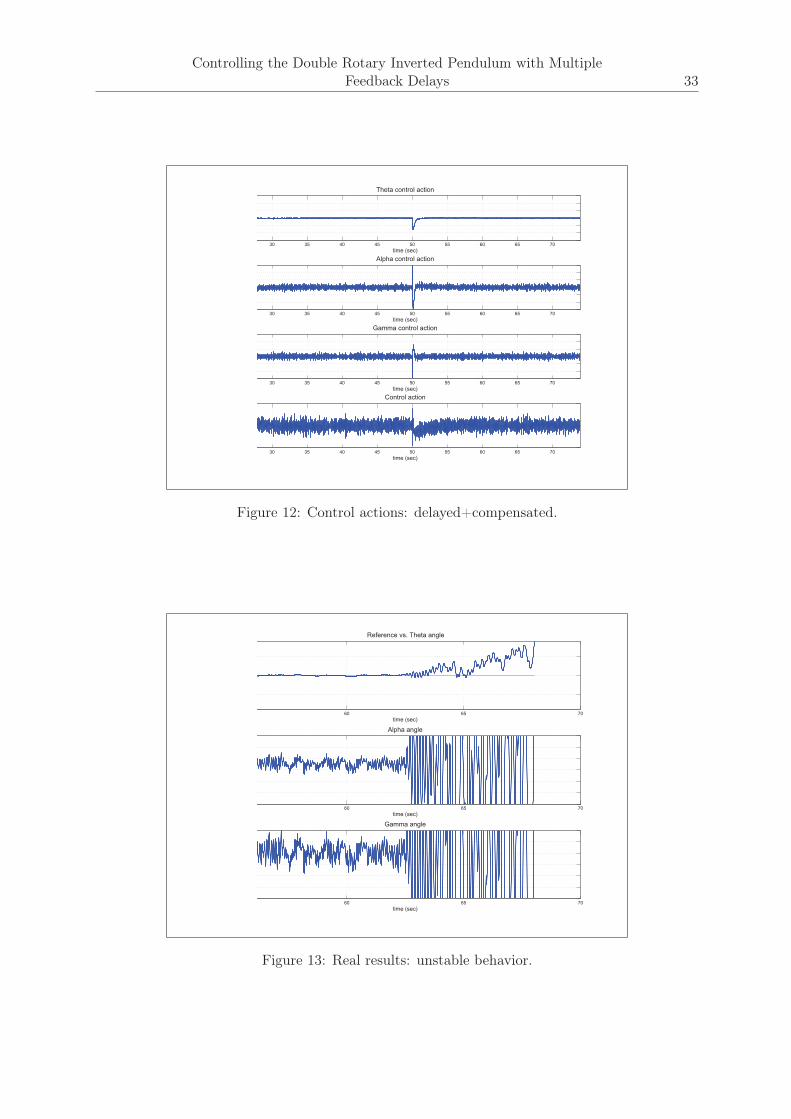
Controlling the Double Rotary Inverted Pendulum with MultipleFeedback Delays 33
30 35 40 45 50 55 60 65 70
Theta control action
time (sec)
30 35 40 45 50 55 60 65 70
Alpha control action
time (sec)
30 35 40 45 50 55 60 65 70
Gamma control action
time (sec)
30 35 40 45 50 55 60 65 70
Control action
time (sec)
Figure 12: Control actions: delayed+compensated.
60 65 70
Reference vs. Theta angle
time (sec)
60 65 70
Alpha angle
time (sec)
60 65 70
Gamma angle
time (sec)
Figure 13: Real results: unstable behavior.
34 V. Casanova, J. Salt, R. Piza, A. Cuenca
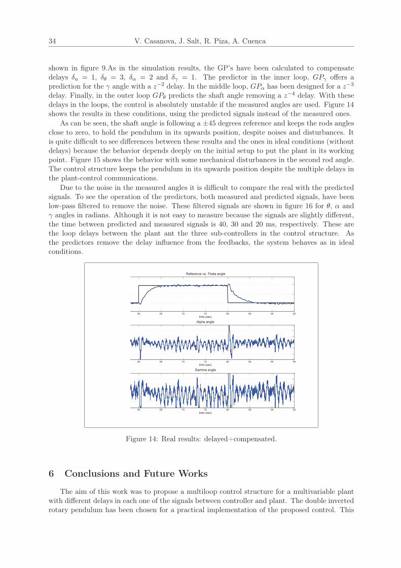
shown in figure 9.As in the simulation results, the GP’s have been calculated to compensatedelays δu = 1, δθ = 3, δα = 2 and δγ = 1. The predictor in the inner loop, GPγ offers aprediction for the γ angle with a z−2 delay. In the middle loop, GPα has been designed for a z−3
delay. Finally, in the outer loop GPθ predicts the shaft angle removing a z−4 delay. With thesedelays in the loops, the control is absolutely unstable if the measured angles are used. Figure 14shows the results in these conditions, using the predicted signals instead of the measured ones.
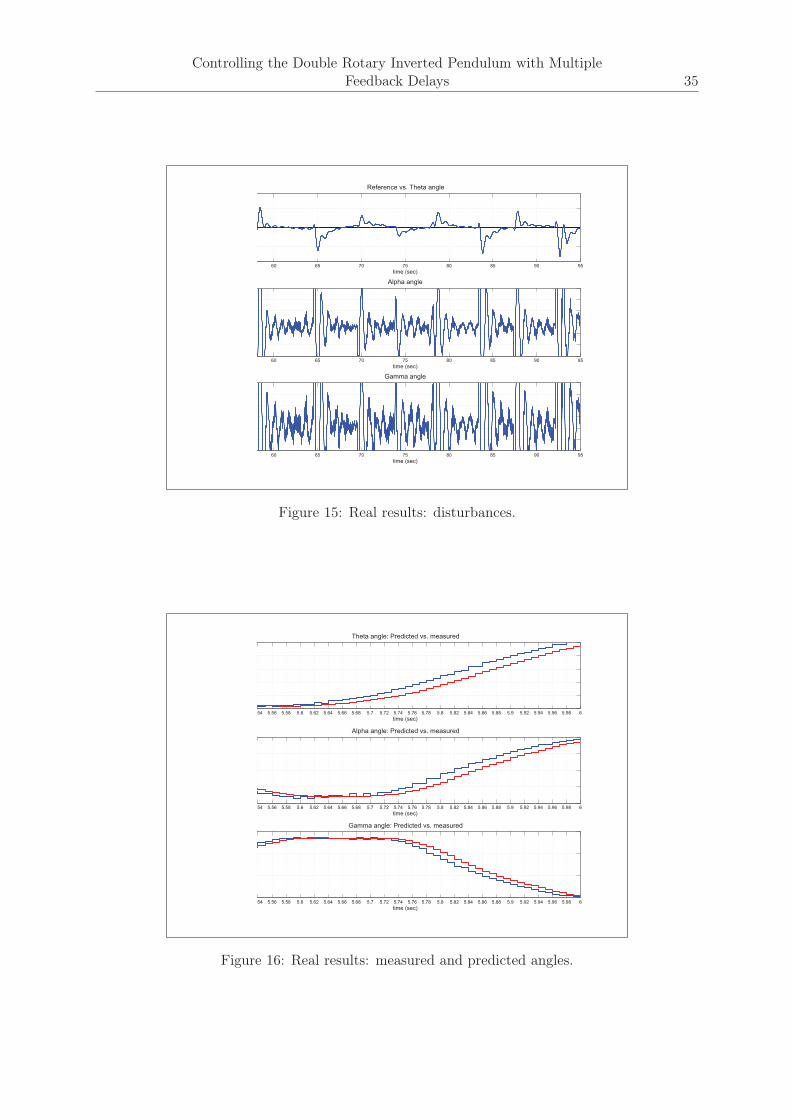
As can be seen, the shaft angle is following a ±45 degrees reference and keeps the rods anglesclose to zero, to hold the pendulum in its upwards position, despite noises and disturbances. Itis quite difficult to see differences between these results and the ones in ideal conditions (withoutdelays) because the behavior depends deeply on the initial setup to put the plant in its workingpoint. Figure 15 shows the behavior with some mechanical disturbances in the second rod angle.The control structure keeps the pendulum in its upwards position despite the multiple delays inthe plant-control communications.
Due to the noise in the measured angles it is difficult to compare the real with the predictedsignals. To see the operation of the predictors, both measured and predicted signals, have beenlow-pass filtered to remove the noise. These filtered signals are shown in figure 16 for θ, α andγ angles in radians. Although it is not easy to measure because the signals are slightly different,the time between predicted and measured signals is 40, 30 and 20 ms, respectively. These arethe loop delays between the plant ant the three sub-controllers in the control structure. Asthe predictors remove the delay influence from the feedbacks, the system behaves as in idealconditions.
60 65 70 75 80 85 90 95
Reference vs. Theta angle
time (sec)
60 65 70 75 80 85 90 95
Alpha angle
time (sec)
60 65 70 75 80 85 90 95
Gamma angle
time (sec)
Figure 14: Real results: delayed+compensated.
6 Conclusions and Future Works
The aim of this work was to propose a multiloop control structure for a multivariable plantwith different delays in each one of the signals between controller and plant. The double invertedrotary pendulum has been chosen for a practical implementation of the proposed control. This
Controlling the Double Rotary Inverted Pendulum with MultipleFeedback Delays 35
60 65 70 75 80 85 90 95
Reference vs. Theta angle
time (sec)
60 65 70 75 80 85 90 95
Alpha angle
time (sec)
60 65 70 75 80 85 90 95
Gamma angle
time (sec)
Figure 15: Real results: disturbances.
5.54 5.56 5.58 5.6 5.62 5.64 5.66 5.68 5.7 5.72 5.74 5.76 5.78 5.8 5.82 5.84 5.86 5.88 5.9 5.92 5.94 5.96 5.98 6
Theta angle: Predicted vs. measured
time (sec)
5.54 5.56 5.58 5.6 5.62 5.64 5.66 5.68 5.7 5.72 5.74 5.76 5.78 5.8 5.82 5.84 5.86 5.88 5.9 5.92 5.94 5.96 5.98 6
Alpha angle: Predicted vs. measured
time (sec)
5.54 5.56 5.58 5.6 5.62 5.64 5.66 5.68 5.7 5.72 5.74 5.76 5.78 5.8 5.82 5.84 5.86 5.88 5.9 5.92 5.94 5.96 5.98 6
Gamma angle: Predicted vs. measured
time (sec)
Figure 16: Real results: measured and predicted angles.

36 V. Casanova, J. Salt, R. Piza, A. Cuenca
is a classic example of multivariable plant whose stability is seriously worsened even with smalldelays. There are four links in the system: one control-plant link (actuator) and three plant-control ones (sensors). The scenario assumes that this four links are a submitted to differentcommunication delays which increases the difficulty to remove its influence on the stability.
A generalized predictor has been used to provide delay-free information for each one of thethree loops in the control structure. Each one has been designed attending to each loop delay.Depending on the quality of the model used in the predictor, the system behaves as in idealconditions, even with one different delay in each of the links. The validity of the proposedcontrol structure has been shown by means of simulated results. The real implementation usingthe Quanser double rotary inverted pendulum shows how the proposed structure works when acertain degree of uncertainty, non-negligible noises and disturbances are present.
The delays in this work have been included in the control structure but they should becaused by the communication between sensors/actuators and the device in which the controlalgorithm is implemented. The goal is to close the loops through a shared communicationmedium (fieldbus, wireless network...), following different paths for each one of the links. Thiswill cause different transport delays in each loop that may be solved with the proposed structure.In this more realistic implementation an additional problem will arise. The unavoidable lack ofsynchronization between the devices (sensors, controllers and actuators) will make the delayvariable and, probably unknown. Some kind of delay identification must be performed or thecontrol structure must be modified to be adaptive to compensate variable (maybe random) delays.
Another improvement of this proposal is to use a plant with more than one input. This willincrease the number of communication links and the number of feedback loops. The 2D invertedpendulum is a good choice to be used in this improvement. This plant increases the degreesof freedom allowing movement in the XY plane. It has two inputs for a planar movement ofthe cart carrying the pendulum. Two measurements of the cart position must be used in thecontroller. The rod can bend in two directions giving two angular measurements. So, the plantoffers a multivariable model (two inputs, four outputs) and, as is also quite sensitive to delays,is an appropriated plant to extend the work in this paper.
Acknowledgement
This work was supported by the Spanish Ministerio de Ciencia y Tecnologa Project DPI2009-14744-C03-03, by Generalitat Valenciana Project GV/2010/018, and by Universidad Polit´ecnicade Valencia Project PAID06-08.
Bibliography
[1] Y. Halevi, A. Ray, Integrated communication and control systems: Part I-Analysis,Journal of Dynamic Systems, Measurement and Control, vol. 110, pp. 367-373, 1988.
[2] A. Ray, Y. Halevi, Integrated communication and control systems: Part II-Designconsiderations, Journal of Dynamic Systems, Measurement and Control, vol. 110,pp. 374-381, 1988.
[3] L.G. Bushnell, Networks and control, IEEE Control Systems Magazine, vol. 21, no.1, pp. 22-23, 2001.
[4] Y. Tipsuwan, M-Y. Chow, Control methodologies in networked control systems,Control Engineering Practice, vol. 11, no. 10, pp. 1099-1111, 2001.

Controlling the Double Rotary Inverted Pendulum with MultipleFeedback Delays 37
[5] P.F. Hokayem, C.T. Abdallah, Inherent issues in networked control systems: Asurvey, Proceedings of the 23rd American Control Conference, Boston (USA), vol.6,pp. 4897-4902, 2004.
[6] T.C. Yang, Networked control systems: A brief survey, IEE Proceedings on ControlTheory and Applications, vol. 153, no. 4, pp. 403-412, 2006.
[7] V. Casanova, J. Salt, Multirate control implementation for an integrated communi-cation and control system, Control Engineering Practice, vol. 11, no. 11, pp. 1335-1348, 2003.
[8] J. Nilsson, Real-time control systems with delays. PhD thesis, Lund Institute ofTechnology, Lund, Sweden, 1998.
[9] J. Nilsson, B. Bernhardsson, B. Wittenmark, Stochastic analysis and control ofreal-time systems with random time delays, Automatica, vol. 34, no. 1, pp. 57-64,1998.
[10] F.L. Lian, J.R. Moyne, D.M. Tilbury, Performance evaluation of control networks:Ethernet, ControlNet, and DeviceNet, IEEE Control Systems Magazine, vol. 21,pp. 66-83, 2001.
[11] F.L. Lian, J.R. Moyne, D.M. Tilbury, Network design consideration for distributedcontrol systems, IEEE Transactions on Control Systems Technology, vol. 10, pp.297-307, 2002.
[12] F.L. Lian, J.R. Moyne, D.M. Tilbury, Modelling and optimal controller design ofnetworked control systems with multiple delays, International Journal of Control,vol. 76, no. 6, pp. 591-606, 2003.
[13] H. Gaoa, T. Chenb, J. Lamc, A new delay system approach to network-based con-trol, Automatica, vol. 44, no. 1, pp. 39-52, 2008.
[14] A.V. Savkin, Analysis and synthesis of networked control systems: Topologicalentropy, observability, robustness and optimal control, Automatica, vol. 42, no. 1,pp. 51-62, 2006.
[15] D.S. Kim et al, Maximum allowable delay bounds of networked control systems,Control Engineering Practice, vol.11, no. 11, pp.1301-1313, 2003.
[16] H. Fanga, H. Yeb, M. Zhong, Fault diagnosis of networked control systems, AnnualReviews in Control, vol.31, no. 1, pp. 55-68, 2007.
[17] O.E. Agamennoni, A.C. Desages, J.A. Romagnoli, A multivariable delay compen-sator scheme, Chemical Engineering Science, vol. 47, no. 5, pp. 1173-1185, 1992.
[18] B.A. Ogunnaike, W.H. Ray, Multivariable controller design for linear systems havingmultiple time delays, AIChE Journal, vol. 25, no. 6, pp. 1043-1057, 1979.
[19] K. Watanabe, M. Ito, An observer for linear feedback control laws of multivariablesystems with multiple delays in controls and outputs, Systems & Control Letters,vol. 1, no. 1, pp. 54-59, 1981.
[20] S. Mori, H. Nishihara, K. Furuta, Control of unstable mechanical system: Controlof pendulum, International Journal of Control, vol. 23 no. 5, pp. 673-692, 1976.
38 V. Casanova, J. Salt, R. Piza, A. Cuenca
[21] K. Furuta, M. Yamakita, S. Kobayashi, M. Nishimura, A new inverted pendulumapparatus for education, IFAC Advances in Control Education Conference, pp. 191-196, 1991.
[22] S. Yurkovich, M. Widjaja, Fuzzy controller synthesis for an inverted pendulum,Control Engineering Practice, vol. 4, no. 4, pp. 455-469, 1996.
[23] W. Zhong, H. Röck, Energy and passivity based control of the double invertedpendulum on cart, IEEE Conference on Control Applications, pp. 896-901, 2001.
[24] J. Driver, D. Thorpe, Design, build and control of a single/double rotational invertedpendulum, The University of Adelaide, School of Mechanical Engineering, Australia,2004.
[25] Quanser Consulting Inc, Rotary experiment #8: Double Inverted Pendulum(DBPEN), 2006.
[26] G. Alevisakis, D.E. Seborg, An extension of the Smith predictor method to mul-tivariable linear systems containing time delays, International Journal of Control,vol. 17, no. 3, pp. 541- 551, 1973.
[27] K. Watanabe, Y. Ishiyama, M. Ito, Modified Smith predictor control for multivari-able systems with delays and unmeasurable step disturbances, International Journalof Control, vol. 37, no. 5, pp. 959-973, 1983.
[28] J.M. Maciejowski, Robustness of multivariable Smith predictors, Journal of ProcessControl, vol. 4, no. 1, pp. 29-32, 1994.
[29] A.M. De Paor, A modified Smith predictor and controller for unstable processeswith time delay, International Journal of Control, vol. 41, no. 4, pp. 1025-1036,1985.
[30] H.J. Kwak, S.W. Sung, I.B. Lee, A modified Smith predictor with a new structurefor unstable processes, Industrial & Engineering Chemistry Research, vol. 38, no. 2,pp. 405-411, 1999.
[31] T. Liu, Y.Z. Cai, D.Y. Gu, W.D. Zhang, New modified Smith predictor schemefor integrating and unstable processes with time delay, IEE Proceedings on ControlTheory and Applications, vol. 152, no. 2, pp. 238-246, 2005.
[32] P. García, P. Albertos, T. Hägglund, Control of unstable non-minimum-phase de-layed systems, Journal of Process Control, vol. 16, no. 10, pp. 1099-1111, 2006
[33] P. Albertos, P. García, Robust control design for long time-delay systems, Journalof Process Control, vol. 19, no. 10, pp. 1640-1648, 2009.