BUREAU OF THE CENSUS STATISTICAL RESEARCH DIVISION REPORT SERIES

SRD Research Report Number: Census/SRD/RR-88102

CONTROLLED ROUNDING OF THREE DIMENSIONAL TABLES

by James T. Fagan

Brian V. Greenberg Statistical Research Division

Bob Hetmnig Economic Programing Division

Bureau of the Census e- Washington, D.C. 20233

This series contains research reports, written by or in cooperation with staff members of the Statistical Research Division, whose content may be of interest to the general.statistical research community. The views reflected in these reports are not necessarily those of the Census Bureau nor do they necessarily represent Census Bureau statistical policy or practice. Inquiries may be addressed to the author(s) or the SRD Report Series Coordinator, Statistical Research Division, Bureau of the Census, Washington, D.C. 20233.

Recommended by: Lawrence Ernst

Report completed: February 12, 1988

Report issued: May 13, 1988 = . ; -. - ;

-.

Controlled Rounding of Three Dimensional Tables

ABSTRACT

The objective of this report is to present a heuristic procedure to find controlled roundings of three dimensional tables. The problem of three dimension controlled rounding is far more difficult than its two dimension counterpart primarily because the underlying network structure of the two dimensional problem does not exist in three dimensions. In fact, given an arbitrary three dimensional table, a controlled rounding may not exist. We present in this paper a heuristic procedure for finding a controlled rounding for three dimensional tables which has been extremely successful under extensive testing.

I. INTRODUCTION

The objective of this report is to present a heuristic procedure to find

controlled roundings of three dimensional tables. The problem of three

dim\nsion controlled rounding is far more difficult than its two dimension

counterpart primarily because the underlying network structure of the two

dimensional problem does not exist in three dimensions. In fact, given an

arbitrary three dimensional table, a controlled rounding may not exist. We -- present in this paper a heuristic procedure for finding a controlled rounding

for three dimensional tables which has been extremely successful under

extensive testing.

After introductory remarks in Section I, Section II begins with a very

explicit description of controlled rounding for a two dimensional table. The

fundamental steps in forming a controlled rounding of a two dimensional table

are to set up a system of linear equations, formulate a network flow problem,

model that system of equations, find a saturated flow through the network and

interpret the flow as a controlled rounding of the original table. In Section

III we begin a similar process for tnree dimensional tables. Up to the stage

of solving a sy-$etn of equations, both problems are structurally identical.

However, we exhibit three dimension tables which fail to have zero-restricted

controlled roundings, weakly zero-restricted controlled roundings, and in fact

any controlled roundings at all. The underlying problem is that in three

dimensions there is no single network as was employed in the two dimensional

case. In Section IV we present a heuristic procedure for finding controlled

roundings of three dimensional tables. The model we introduce is based on a

-2-

sequence of network flow problems; the solution of each reduces the size of

the table to be rounded. We then extract a controlled rounding of the

original table from this sequence of solutions to the individual network flow

problems. In Section V we discuss software developed at the Census Bureau to

implement the heuristic procedure introduced in the preceeding section and

report on program performance. In Section VI we describe an alternative

definition of controlled rounding and discuss programs to implement the

alternative procedure. Lastly, Section VII is a brief summary of findings.

We continue this introduction by establishing terminology, notation, and

definitions to lay the groundwork for describing procedures for finding a

controlled rounding for two dimensional tables. Most simply stated, the

problem is as follows.

. Given a positive integer k and an additive table of non-neqative integers

* “00 PO1 “02 l ** “oc

alo “11 a12 l ** “1c A= a20 a21 a22 l ** a2c

. . . . . . .

l . . ... .

.

I

. . ... .

"RO I "Rl aR2 . . . aRc 9

that is,

C

c j=l

aij = '10

=R-- -XI * ai j' aoj

i-l

"ij 2'

i=l s**.* R

j=l s***, C

i-l ,...,R and j=l,...C

find an additive table

-3-

boo

b10

b20 B . =

.

.

bRO

where

.

b01 b02 l ** hoc

%l b12 l ** blC

.b21 b22 l ** bzc . . . . . .

. . . . . .

. . . . . .

bR1 bR2 l a. bRC

I

C c b.. = biO

j=l lJ .. i-l s---s R

j=l ,...,C and

(1) bij = [aij/bIb or [aij/blb+b i=O,...,R j=O,...,C,

where [x] stands for the greatest integer less than or equal to x. Such a

table B is called a controlled rounding of A. If we replace (1) by

(2) lbij - 'ijl < b

we say B is a zero-restricted control led rounding of A. Under a zero-

restricted cont_r.$jed rounding, no multiple of the base changes. If we

replace (1) by -.-* *

(3) Caij/blb or [aij/bIb+b if a.. > 0

bij t 73

0 if a.. = 0 1J

we say B is a weakly zero-restricted controlled rounding of A.

-4-

All two dimensional tab

under many circumstances one

rather than one that is not

es have zero-restricted controlled roundings, and

prefers a zero-restricted controlled rounding

ero-restricted, for example, in order to obtain

an unbiased controlled rounding, see (Cox, 1987). When seeking a controlled

rounding that is minimal with respect to some measure of closeness, zero-

restricted controlled roundings do not suffice as discussed in (Greenberg,

1988). There exist three dimensional tables which have controlled roundings

yet fail to have zero-restricted controlled roundings, so for three

dimensional tables controlled rounding procedures must be developed which are

not necessarily zero-restricted. Of course, if zero is to change, it can only

always positive. The added definition,

weakly zero-restricted, recognizes the special role of zero. That is, under a

ing zero is always to remain zero, but a

ease by the value of the base.

go to k since a controlled rounding is

- weakly zero-restricted contolled round

non-zero multiple of the base can incr *

II. STEP-BY-STEP PROCEDURE FOR SOLVING THE TWO DIMENSIONAL CONTROLLED

ROUNDING PROBLEM

In this Section, we go though a step by step procedure for finding two

dimensional (not necessarily zero-restricted) controlled roundings --

including a step in which the problem is reduced to the solution of a zero-one

network flow problem. This being done, we set the stage for the formulation

of a heuristic solution to the three dimensional controlled rounding

problem. The presentation here follows closely along the lines of (Greenberg,

1988). For a further discussion of the two dimensional problem, we refer the

reader to (Cox and Ernst, 1982) and (Cox, 1987).

One first reduces the problem modulo the base. That is, write

(4) A= bD + R

: . -- -. - ;

where D and R ire RxC matrices and

a ij

= bdij+ r.. ‘J

where 0 < r.. < b for i=l,...,R and j=l - 1J s*-*s c.

-5.

Define

and

.

C d iOxE " d

j=l ‘J i=l ,***, R

R

dOj = iil dij j=l ,***, C

R C R C do0 = C c dij =i~l di0 = c

i=l j=l j-l dOj

C

‘10 = ’ ‘ij j=l i=l ,...S R

R

rOj = ifl rij j=l ,***, C

R C roO = C C rij = f r

iR1 10 = c r..

if1 j=l jcl OJ f

With these added definitions, we have additivity of the following system of

tables--including marginal positions:

do0 a01 a02 l ** aoc do0 do1 do2 l ** dot

a1o a11 a12 l ** a1c %o dll d12 . . . dlC

a2o a21 a22 . iif0 a2c d20 d21 d22 l ** d2C . . . . . . . =(b) . . . . . . . +

. . . . . . . . . . . . . .

aRO aR1 aR2 l *= aRC I

dRO I

dR1 dR2 l ** dRC

roe r01 r02 l l * rot

qo q1 r12 l ** rlC

r20 r21 r22 l ** r2c . . . . . . .

. . . . . . .

. . . . . . .

rRO rR1 rR2 l ** rRC '

so equation (4) applies to the entire tables.

-60

Forming a (zero-restricted, weakly zero-restricted) controlled rounding, S of

R, the sum

B = bD+S

will be a (zero-restricted, weakly zero-restricted) controlled rounding of

A. Thus, our objective is to form a controlled rounding of R noting

that r.. <b fori=l

&,

,...,R and j=l,...,C.

"fold-in" the RxC table R to form an R+l by Ctl table in which all

marginals are multiples of the base by adding a slack row and slack column.

That is, we form the table

.

Coo *

Cl0 C = C20

.

.

.

CRO

'R+l,D

Co1 co2 . . . Cot Co ‘01

Cl1 _- Cl2 . . . ClC Cl ‘01

C21 c22 . . . C2C C2 ‘01 . . . . . . .

. . . . . . .

. . . . . . .

CR1 CR2 . . . CRC CR ,C+l

‘R+l,l CR+1,2 l ** CR+l,C CR+l,C+l

where

C ij = rij

i=l ,...,R and j=l,...,C

cl ,ctl = C( : c Wlb+b j=1 iJ - t" c . jcl ‘J

i=l,*.*,R

= - -- -. - ;

1.

R R

CR+l,j s [tic1 cij)/bIb+b I oifl Cij jfl,...,C

C R C

‘Rtl,Ctl = ’ .f ’ ’ iRl J 1 = 0 IJ

-7.

C Cl0 = [( C cij)/bIb+b

jfl i-l s-•*, R

C

CRt1,O = jfl ‘R+l,j j=l ,...,C+l

R

co,ctl = if1 'i ,Ctl i=l ,...,Rtl

Rtl Ctl Rtl C+l coo = c c

i=l j=l 'ij = iil '10 = jfl �Oj l

Note that all marginal values of C are multiples of &

Let us take a 4x4 table, A, and follow the steps through to this point

with rounding base b-3:

119 24 40 18 37 102 21 33 15 33 17 3 7 3 4

15 4 8 3 0 12 3 6 3 0 3 1 2 0 0

A= 41 7 13 1 20 3D= 36

6 12 0 18 R= 5 1 1 1 2 19 1 5 9 4 15 0 3 9 3 4 1 2 0 1

44 12 14 5 ,13 39 12 12 3 12 t

5 0 2 2 1

It is easy to see that

and

A= 30 + R

-80

36 6 9 6 6 9

612003

C- 611121

612012

602211

12 3 2 3 2 2.

Returning to the main development, our objective is to reassign values for

Cij for i=l,...,R+l and j=l,..., C+l as either 0 or b while maintaining

additively to the marginals. Having done this, and calling the new values fij

and the new table F (with the same marginals as C), observe

. Coo Co1 co2 . . . Cot co ,C+l

Cl0 fll fl2 . . . flC fl '01 I c20 f21 f22 l ** fzc f2,Ctl

F . = . . . . . . .

. . . . . . . .

. . . . . . . .

'RO fR1 $2 . . . fRC fR,C+l --

CRt1,O fRtl ‘1 fR+1,2 l ** fR+l,C fRtl ,C+l

is a controlled rounding of C.

To be somewhat more formal, we solved the following system of equations

for fij for I=1 ,..., R+l and j=l,..., C+l:

Ctl c f.. = cio

j=l ‘J i=l ,...,R+l

Rtl y- _

c f..=c 1J Oj

j=l ,...,Ctl i=l

f ij c EOsbl i=l ,...,Rtl and j=l,...,Ct1.

-90

This system does have solutions, and one of the ways to find a solution is to

obtain a saturated flow through the complete directed bipartite capacitiated

network shown in Figure 1, see (Cox, Fagan, Hemmig, Greenberg, 1986 and

Gondran arrd Minoux, 1984). Nodes correspond to marginal constraints, all arcs

flow from left to right, and the directed arc between node nio and noj

corresponds to cell (i,j) in table C, cij, where i=l,...,R and j=l,...,C.

ROWS COLUMNS

/b

lb

,C+tb

FIGURE 1

The nodes on the left correspond to sources, nodes on the right

correspond to sinks, supplies (row marginal values) and demands (column

marginal values) are shown alongside each source and sink respectively, and

each arc has upper capacity equal to one. A saturated flow does exist, and we

set fij equal to the flow over arc (KS noj) times h

-lO-

The table

fOO f01 f02 l ** foe

50 fll fl2 . . . flC

S = f20 f21 f22 . . . f2C

. . . . . . .

. . . . . . .

. . . . . . .

fRO fR1 fR2 . . . fRC

where

. C

f i0

= c f.. j=l ‘J .

i-l R s--*9

*

R

fOj = ifl fij j=l s***s R

R C foO = c c fij =

i=l j-1

is a controlled rounding of R and

B = bD+S

is a controlled rounding of A.

Continue with the base 3 example started earlier:

119 24 40 18 37 102

15, 4 8 3 0 12 z.. ; A= 41'; 7 13 1 20 30 = 36

19 15 9 4 15

44 12 14 5 13 39

21 33 15 33

363 0

6 12 0 18

0 39 3

12 12 3 12

-11.

17

3

R = 5

4

5

3 7 3 4 36 6 9 6 6 9

1 2 0 0 6 1 2 0 0 3

1 1 1 2 C= 6 1 1 1 2 1

1 2 0 1 6 1 2 0 1 2

0 2 2 1 6 0 2 2 11

12 3 2 3 2 2.

Obtain a base 3 controlled rounding, F of C, extract the upper left RxC

subtable with derived marginals, S, (which will be a base 3 controlled

rounding of R), and form

B =3DtS .

which will be a base 3 controlled rounding of A. Below we display five base

3 cbntrolled roundings, .F of C, the corresponding controlled rounding,

S of R, and finally the controlled rounding, B of A (which was our

objective all along).

Fi -

1.

36

6

6

6

6

12

2.

36

6

6

6

6

12

6 9 6 6 9

0 3 0 0 3

3 0 0 3 0

0 3 0 0 3

0 0 3 3 0

3 3 3 0 3

= - -0 -. - ;

691669

3 3 0 0 0

0 3 0 0 3

3 0 0 3 0

0 0 3 0 3

I03333

18

3

6

3

6

Si -

Bi -

3 6 3 6 120 24 39 18 39

0 3 0 0 15 3 9 3 0

3 0 0 3 42 9 12 0 21

0 3 0 0 18 0 6 9 3

0 0 3 3 45 12 12 6 15

18 6 6 3 3

6 3 3 0 0

3 0 3 0 0

t

6 3 0 0 3

3 0 D 3 0

120 27 39 18 36

18 6930

39 6 15 0 18

21 3 3 9 6

42 12 12 6 12

-12-

3.

36

6

6

6

6

12

69669 l&

00033 3

03003 3

03300 6

33000 6

3 0 3 3 3

3 9 3 3 120 24 42 18 36

0003 15 3 6 3 3

0300 39 6 15 0 18

0330 21 0 6 12 3

3300 45 15 15 3 12

One can see that each of the tables in the "B" column is a base 3

controlled rounding of A. Note that BI is a zero-restricted controlled

rounding, B2 is weakly zero-restricted, and B3 is the only table in which a

true zero is given the value 3. In all, a wide range of possible roundings

exist.

III: CONTROLLED ROUNDING--IN THREE DIMENSIONS

In Section II, we defined two dimensional controlled rounding, showed how

it can be couched as a solution to a set of linear equalities, and finally how

to' find the solution by solving a zero-one capacitated network flow problem.

In this Section we define the three dimensional controlled rounding problem

and show how the exact solution found in two dimensions fails to extend to

three dimensions. In the following chapters we carefully develop a heuristic

procedure to solve the three dimension controlled rounding problem. We begin

by establishing notation, terminology, and appropriate definitions. As will ,

be observed, the structure and setting up of the three dimensional problem is

identical to the two dimensional problem. The major departure arises when we

must solve the derived system of equations to find the actual controlled

rounding.

A simple way of representing an RxCxL three dimensional table is shown

below. Above%t&dashed line we have the two dimensional levels k=l,...L

adding to the totals face below the line.

w

w

W

I E

Nr

. .

.+-

+- w

w

. .

. Z

K

c- .

. .

. .

.

W

z W . .

W

w

w

g .

. .

gg

W

@

I

I; I

0”

r; W

%

. . b

0 z

W

F 0

W

W

g .

. .

N-

!s

. .

W

w

w

iz

. .

. E

Z

N

NN

.

. h,

. W

E

2

0

. .

. .

. .

. .

. .

. .

W

w

w

i?

Iu

E

z-

. . .

W

. . l N

F

0”

F w

z 7

. .

. W

z I-

W

s

W

z I-

. . h,

z l-

. . . . . .

. . . =

_ ;

-.

- ;

-.

. .

. W

5

w

F

K

r-

-14.

WHERE

(5)

(6)

(7)

.

(8)

(9)

(10)

(12)

L

aijk =

jcl iJk a. =aiOk

=

i=l ,...,R and j=l,...,C

i=l ,...,R and k=l,..., L

R

iil "ijk = 'Ojk j=l ,...,C and k=l,..., L

' 2 "ijk I=1 ,...,R j=l,...,C k=l,...,L

jcl OJk

R c a. = = ifl 'iOk = 'OOk

L R

kil "Ojk =ifl aijO = 'OjO

L C

kfl 'iOk = jfl 'IjO = "iO0

k=l L s***s

j=l C s***s

I=1 R s***s

R C L

& "100 tjfl aOjO =kfl aOOk" '000

= - -- -. - ; -:

-150

Given a positive integer, b, the objective is to find a three dimensional

additive table, B, (adapting the representation and notation used for A above)

which satisfies (5).(12) and

(13) bijk=[(aijk/b]b or [(aijk/b)lb+b i=O,...,R j=O,...,C, k=O,...L'

where [ ] is the greatest integer function.

In this paper we present a heuristic iterative procedure which starts

with a three dimensional table A and rounding base b and attempts to find a

controlled rounding 8. If no solutions are found after a specified number of

iterations the program indicates its inability to find a solution. As is

. shown by several examples in Section IV, there exist tables A and rounding

base b for which solutions to the system of equations above do not exist.

Thsse are carefully contrived examples. All three dimensional tables we have

encountered through a random generation process or based on actual 1980

Decennial Census tabulations do have controlled roundings. Except for

specially constructed examples, under extensive testing this heuristic has

always yielded controlled roundings in an efficient manner.

We begin exactly as in Section II. If A is an RxCxL table, write

(14) A= bD + R

where D and R are also RxCxL tables and

aijk = bdijk + rijk

where 0 2 rijk < b for i=l,...,R j=l ,...,C and k=l,..., L.

Defining z . -- -. - ; -.

d ij0' diok, d Ojk' diOOs dOjO' d00k' dOOO

r ij0' riOk' rOjk' riOO' 'OjO' r0Ok' rOOO

as one would expect, we can extend the additivity in (14) above to include

marginal positions. If we form a (zero-restricted, weakly zero-restricted)

-16-

controlled rounding, S and R, the sum

B =bDtS

is a (zero-restricted, weakly zero-restricted) controlled rounding of A.

Thus, our objective reduces to finding a controlled rounding of R observing

that r.. 1Jk

< b for i,j,k > 0. From this point onward, without loss of

generality we can assume that b=l and c.. JJk

< 1 for i,j,k > 0 by dividing all

entries in the table R by b. We continue under this assumption.

Next, "fold in" the RxCxL table R to obtain the (R+l)x(C+l)x(L+l) table C

where:

. Cijk = rijk i=l R s***s

L L c. 1 ,j ,Ltl = CkEl 'ijkl ’ 1

= -& ‘ijk

'1 ,C+l,k = C E 'ijkl ' 1 -c c.

j-l jcl ‘Jk s

‘R+l,j ,k =s c R

i=1 W ]tl

-i4, 'ijk

'i ,C+l,L+l = j'l kkl 'ijk - 'jam kil 'ijk' I

j=l ,...,C k=l,...,L

i-l ,.'..,R j=l,..., C

i=l ,...,R k=l,..;,L

j=l ,...,C k=l,...,L

i=l s***s R

‘Rtl, j ,Ltl = iI, k!l ‘ijk j=l,..*,C

‘Rtl ,C+l ,k = II, jI, 'ijk - [ ~ ~ Cijk] k=l,...,L

if1 j=l

R C L

CR+l,Ctl,Ltl = [ ’ ’ ' 'ijk] ' ' - i!l jil k!l 'ijk i=l j=l k=l

'ijo = Ckkl 'ijkl + 1 P

‘iok = C ~ Cijk] ’ 1 j-1

COjk = [ i Cijk] + 1 i=l ,

L

'iO0 = kfl 'iOk = 4 ' * jcl ‘JO

L R .

'OjO = kfl 'Ojk = if, 'IjO

I

L --

Cook = f c ' = kfl 'iOk jCi OJk

R+l Ctl L+l

cooo = c i-1 j:l k=l ' 'ijk

Rtl Ltl Rtl Ltl

i=l ,...,R j=l,...,C

i=l ,...,R k=l,...,L

j=l ,...,C k=l,...,L

i=l ,.-es R

j=l C ,***s

k=l L s-*.9

R+l Ctl

R+l C+l L+l

= if1 'iO0 = jfl 'OjO = kfl 'OOk .

As can be seen, this is simply the more complicated counterpart of the C

table defined in Section II used with two dimensional controlled rounding.

Let us take a 3x3x3 table and follow the steps through to this point. Suppose

the base b=3,~qd;the table A is as follows:

60 ! 17 24 1-i

28 8 7 13

A = 12 9 2 1

20 015 5

52 19 14 19

13 0 310

t

24 11 8 5

15 8 3 4

-180

51 15 21 15

24 6 612

3D= t 9 9 0 0

18 015 3

42 15 12 15

12 0 3 9

t

18 963

12 6 3 3

10 4 2 4

1 0 0 1

t

6 2 2 2

3 2 01

33 12 9 12

t

I 15 6 3 6

12 6 0 6 I

6 0 6 0 I

As discussed above, we seek a base 3 controlled rounding, S of R. Before

4 0 3

I 0 01

2 0 0 I

2 0 2

I

26

6 11

9

10 5 11

2 1 3

4 4 3

4 0 5.

. creating the C table, we divide all entries in R by b=3 to reduce the problem

to one in which all marginals are integers and all internal entries of C are

les than or equal to one. Having done this, we get C:

317 7 g 8

6 1 1 2 2

9 2 2 2 3

, t

7 2 1 2 2

9 2 3 3 1.

The objective is to replace all internal entries of C with the values zero or

onewhile mair$aining table additivity to the marginals. So doing provides a

controlled rounding, F of C, as in Section II , which leads to a controlled

rounding, B of A. In the next section a heuristic procedure is provided for

finding F. Below one such zero-one assignment is displayed, and this example

is continued to obtain a controlled rounding of A. One controlled rounding, F

of C is:

-19-

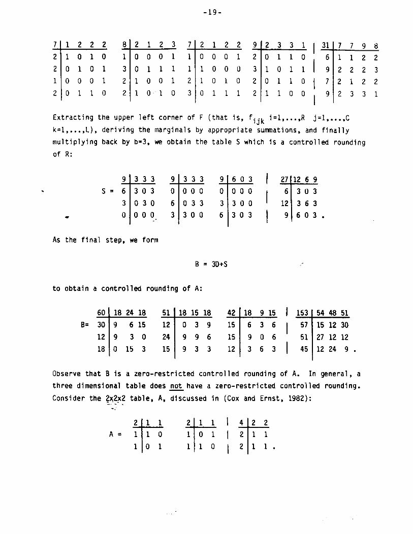
Extracting the upper left corner of F (that is, fijk i=l,...,R j=l,...,C

k=l ,...,L), deriving the marginals by appropriate summations, and finally

multiplying back by b--3, we obtain the table S which is a controlled rounding

of R:

As the final step, we form

B= 3D+S --

to obtain a controlled rounding of A:

Observe that B is a zero-restricted controlled rounding of A. In general, a

three dimensional table does not have a zero-restricted controlled rounding.

Consider the 2~2x2 table, A, discussed in (Cox and Ernst, 1982): -. -- ;

-2o-

This table does not have a zero-restricted controlled rounding base 2, however

a weakly zero-restricted controlled rounding does exist:

B=F ,E;,E.

The following 6x4x3 table fails to have a zero-restricted or a weakly zero- - restricted base 1 controlled rounding:

ii 1 1 1 1 Q

1 0 l/2 0 l/2 0

1 l/2 0 l/2 0 0

l G=O 0000 1

0 0000 1

4 l/2 l/2 0 0 !*

1 0 0 l/2 l/2 1

1111 Q

do00 1

0000 1

l/2 0 0 l/2 1

0 l/2 l/2 0 1

l/2 l/2 0 0 0

D 0 l/2 l/2 0

1 1 1 1

0 l/2 0 l/2

l/2 0 l/2 0

l/2 0 0 1/a

0 l/2 l/2 0

0 0 0 0

0 0 0 0

3 3 3 3

0 1 0 1

1 0 1 0

1 0 0 1

0 1 1 0

1 1 0 0

0 0 1 1.

The most direct way to see that G does not have a zero-restricted controlled

rounding is to consider the system of equations

6 7

ii1 Xijk = gojk j=l,~~~,4 k=1,...,3

(!I

'ijk = giok j=l,..., 6 k--l,..., 3 j=l

(gijk* 0)

-21.

Xijk = gij0 i=l 9.--s 6 k=l

j=l 4. ,*a*,

A zero-one solution to this system would be a zero-restricted controlled

rounding of G. However, by writing this system in matrix form,

DX = E,

one can verify that the matrix D is non-singular. The original table entries

gjjk (i,j,k > 0) are the only values which satisfy this system (i.e., allow

for an additive table). Thus, A cannot have a zero-restricted controlled

rounding. This example was suggested to us by Gale (1987) and is based on a

multicommodity flow problem failing to have integer solutions discussed in

(Gale, 1960, pp. 173-174).

. To show that G cannot have a weakly zero-restricted controlled rounding

we proceed as follows. First observe that if B is any controlled rounding of

G,then boo0 must equal 13. For otherwise all marginal values of B would be

the same as marginals of G and hence all zeros of G would also be zeros of B;

and we saw above that the table G is the only table satisfing those marginals

with zeros as they are placed in G. Thus bODD = 13.

If boo0 = 13, one of bOG2, and must equal and the

two must 4. Assume = 5, = boo3 4 and the zero in

G remain zero B. To B one complete the completed

table

5 4

b121 0 0 b211 b231 o

0 0 0 1

0 0 1

b511 o o 0 0 ’ be41

Level 1

1 1 4 0 0 0

0 0 0 1

o o 1

0 b432 o

b512 b522 o 0

0 b632 0

t

t

~

Level 2

1 1 1 1

0 b123 0 b143

‘213 o b233 o

‘313 O 0 b343

0 b422 b433 0 0 0 0 0

0 0 0 0

Level 3

-22-

where bljk@S denote values to be assigned. Note that b312 + b313 11 since

b310 L 1 and b311 = 0, so b312 or b313 must equal 1. By setting b312 = 1,

there is only one way to complete Level 2:

4

0

0 1 1

1

1

1

1111 4

0 0 0 0 1

0 0 0 0 1

1 0 0 0 1

0 0 1 0 1

0 1 0 0 0

0 0 0 1 0

1 1 1 1

0 0 0 1

0 010

1 0 0 0

0 1 0 0

0 0 0 0

0 0 0 0

Level 2 Level 3 .

Si rRe b420 1 1 and b421 =:b422 = 0, then b423 must be set to 1 leading to a

unique Level 3 shown above. But b341 t b342 + b343 = 0 < b340 = 1. Thus, one

cannot assign b312 = 1. A similar analysis shows that b313 cannot be set to 1

so that bOOl cannot be set to 5. A comparable analysis shows that neither

bOG2 nor boo3 can be set to 5 while leaving zeros in G remain--as zeros in B.

Accordingly, there is no weakly zero-restricted rounding of G.

However, a controlled rounding of G does exist, namely:

5 2111 5

1 0100 0

1’ 1000 0 r 0 0000 1

0 0000 1

1 1000 1

1 1 1 1 4 1 1 1 1

0 0 0 0

0 0 0 0 1 0 0 1 0

0 0 0 1

+ 1 0 0 0 1

1 1 0 0 0

0 0 1 0 1 0 1 0 0

0 1 0 0 0 0 0 0 0

1 0 0 0 0 0 0 0 0

2 1 0 1 0

2 1 0 0 1

2 0 1 1 0

2 1 1 0 0

3 10 11. 2 I

0011 1 = - -- -. - ;

Note zeros chat&d to ones are in positions (6,1,2) and (6,1,0). Six marginal

integer positions are increased by one, namely:

-23.

The controlled rounding exhibited here was obtained using software

developed by the authors at the Census Bureau based on the three dimensional

heuristic which we discuss in the next section.

Not all three dimensional tables do have a controlled rounding, and over

the next several pages we present a procedure for constructing tables failing

to have a controlled rounding due to Ernst (1987). Start with the following

three dimensional table, E, found by Ernst working independently:

By employing an analysis as for the example above, one can see that there does

not exist a controlled rounding which leaves all zero values fixed. However,

there does exist a controlled rounding, H1 of E, shown below, and using

arguments similiar to those above for the Gale example, G, we observe that for

every controlled rounding of E, the grand total, EooO rounds to 2:

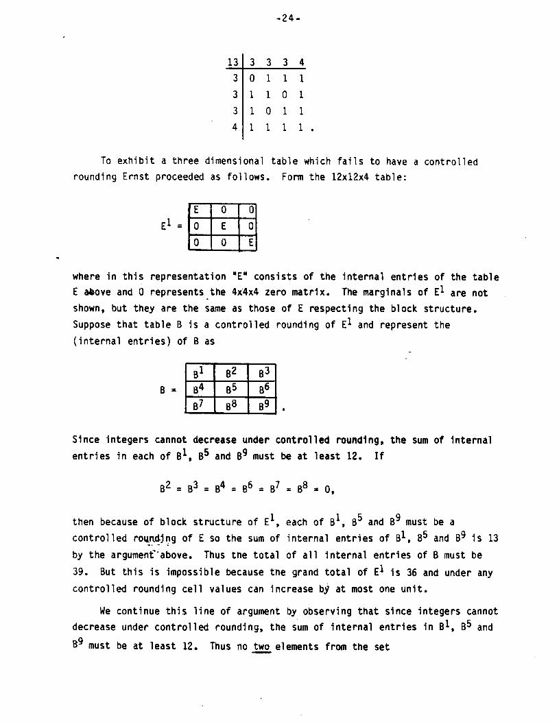
-24.

13 3 3 3 4

3 0 1 1 1 I- 3 1 1 0 1

3 1 0 1 1

41111.

To exhibit a three dimensional table which fails to have a controlled

rounding Ernst proceeded as follows. Form the 12x12~4 table:

.

where in this representation "E" consists of the internal entries of the table

E beove and 0 represents the 4x4x4 zero matrix. The marginals of E1 are not

shown, but they are the same as those of E respecting the block structure.

Suppose that table B is a controlled rounding of E1 and represent the

(internal entries) of B as

B =

Since integers cannot decrease under controlled rounding, the sum of internal

entries in each of B1, B5 and Bg must be at least 12. If

B2 = 83 = 84 = B6 = B7 = B8 = 0,

then because of block structure of El, each of B', B5 and Bg must be a

controlled roundjng of E so the sum of internal entries of B1, B5 and Bg is 13 -. - ; by the argumenf'above. Thus the total of all internal entries of B must be

39. But this is impossible because the grand total of E1 is 36 and under any

controlled rounding cell values can increase by at most one unit.

We continue this line of argument by observing that since integers cannot

decrease under controlled rounding, the sum of internal entries in B1, B5 and

Bg must be at least 12. Thus no two elements from the set

-25.

{B2 B3 B4 B6 B7 B8)

can contain a one. Hence exactly one element from that set must contain a one

based on the discussion above. Without loss of generality we can assume that

B2 contains a single one, and so because of the block structure of B, Bg must

be a controlled rounding of E. Thus the sum of internal entries of Bg must

equal 13 and (as by the arguments above) the sum of all elements of B must

equal 38. This also contradicts the fact that B is a controlled rounding of

El. As all possibilities have been examined, we can conclude that El has no

controlled rounding.

To create a smaller three dimensional table which fails to have a

. controlled rounding we form the 8x8x4 table, E2,

where "E" in this representation consists of the internal entries of table E

and 0 is the 4x4x4 zero matrix. The marginals of E2 (not shown) are the same

as those of E respecting the block structure, and the totals face of E2 (Level

0) is:

24

3

33333333

01110000

11010000

10110000

11100000

00000111

00001101

00001011

00001110.

Let B be an arbitrary controlled rounding of E2 and write the internal

entries of B (in block form) as:

-26.

and let

4 4 4-

$00 = c r: C bfjk S=l,...,4 , i=l j=l k=l

with other marginals defined similarly. Note that

4 and boo0 =

2 3 If boo0 = boo0 = 0, then B1 and B4 are both controlled roundings of E1 so

. 1

bOOO = bioo =

whych contradicts the fact that

bkoo + bZ00 = 2 3 The totals boo0 and boo0 cannot both

the relation

13

booo 1. 25.

be greater than zero since, once again

bOOO %,il b ioo 5 25 s

will be violated. Without loss of generality we can assume that

and let

2 bOOO

3 = 1 and boo0 = 0,

= _ -- -. - i - :

b2 1 iljlkl’

for a unique l<i < 4, lcj < 4, and l:klL 4 and - l- - l-

bijk = 0

otherwise. It follows that

-27-

and

If

then

. and as

I b1 iOk =

Id be a control 1

impossible. Thus, we

B1 wou

b iOk

eilOkl = 1 and b! 1 10kl= 1

biOkE{O'l) for (i,k)t(il,kl) i=1,...,4 k=1,...,4,

ed rounding of E with bioO = 12, which as shown above is

can assume

1 4 boo0 = boo0 = 12s

= biOk = eiOk (i,k)#(il,kl), i=l,.

b. ’ Pkl

= 2

,4 k=1,...,4. . . !

bilOkl = "

and so

If

eilOkl =0

then B1 would be a controlled rounding of E with bkoo = 12, which, once again

is impossible. Thus, assume

= - -- -. - ; -.

eilOkl = 1.

-280

Since no marginal values of E2 can decrease under a controlled rounding,

b'. 1 iJ0 = eijO

and bojk f eojk i=1,...,4 j=1,...,4 k=1,...,4.

Thus

, 4 3 4 1 4 b; oo= 7 bt

1 j&l ‘lok = 1 bi jo=

j=l 1 .I ei jo= eiloo (~3)

J=l 1

and so there exists lLko 5 4 such that kg+ kl and

b: 10kO= ei Ok + '* 1 0

- But

1 4 1 * bOOkO = iLlbiOk

4 1 o = jzlbOjko = eOjkos egOkO (=3)s

so there exists, O<i -O-

< 4 such that iof il and

1 bi OOkO = eiOOkO - '*

However, by construction, since

iof iI and ko# kl,

it follows that

biojko = 0 for all j=5,...,8

and so = . : -. - -

1. 1 bioOko = biOOkO < eiOOkO

-290

This would be a contradiction

under a controlled rounding.

rounding.

The fact that example E2

difficult to see than for.El,

possible having no controlled

conjectures seem plausible.

of the fact that integer values cannot decrease

Thus the table E2 fails to have a controlled

failed to have a controlled rounding was more

however, we did want to find as small a table as

rounding. In addition, the following

Conjectures: Every three dimensional table with integer marginals having at

least one dimension less than 4 does have a controlled rounding. Every table

having fewer than 256 interior cells does have a controlled rounding.

A rather subtle extension of the examples above, EI and E2, was also

w observed by Ernst (1987). We couch the discussion in terms of E2. Note there

are 256 internal cells in E2, and let B = l/300. Form the table E3 having

intlernal entries

3 eijk

2 = eijkt '

and derive marginals by addition. All table values of E3 (including

margi nals) fail to be integer, in fact,

2 3 eijk < eijk

2 < eijk + 1.

One can see that E3 fails to have a controlled rounding by noting that any

controlled rounding of E3 is also a controlled rounding of E2. The table E3

differs from E2 to the extent that no entries of E3 are integers. That is,

the failure of E2 to have a controlled rounding is not a function of the

behavior of integer table values under controlled rounding.

We couldhave used the Gale example, G, rather than the Ernst example, E

in constructin-&counter examples by forming

-300

and

G2=

and using the identical analysis show that G1 and G2 fail to have a controlled

rounding. The crucial factor is that for every controlled rounding of both E

and G, the grand totals, eOO0 and ~000, must increase by one unit. By

letting c = l/400 we could have defined G3 where .

3 2 gijk = gijk ' c

and obtained another non-integer table failing to have a controlled rounding.

Even though there do exist three dimensional tables which have no

controlled roundings, they must constitute rather rare events. After randomly

generating many three dimensional tables and also examining tables that arise

in real applications as will be discussed below, all were observed to have

controlled roundings.

IV. FINDING CONTROLLED ROUNDINGS IN THREE DIMENSIONS

In Section III, we started with an RxCxL table, A, for which we wish to

find a controlled rounding and derived an (R+l)x(C+l)x(L+l) table, C, having

integer marginals and internal entries less than or equal to one. If we

assign zeros and ones to the internal entries of C and maintain additivity to

the marginals, the revised table will lead to a controlled rounding of A as in

Section II. W-objective of this section is to develop procedures for such

an assignment. -'For ease of exposition, notation, and diagram drawing, we let

C be of size 4x3~3. It will be clear how this procedure plays out for

arbitrary R, C and L greater than or equal to 2. Let C be written:

-310

*cOll*c021*c031 coo2

clll c121 %31 *c1o2

‘211 ‘221 ‘231 *c202

‘311 ‘321 ‘331 *‘302

‘411 ‘421 ‘431 ‘402

*c012*c022*c032 coo3 I *‘013 *‘023 *‘033

I ‘112 ‘122 ‘132 *‘lo3 ‘113 ‘123 ‘133

‘212 ‘222 ‘232 *‘203 ‘213 ‘223 ‘233

‘312 ‘322 ‘332 *‘303 ‘313 ‘323 ‘333

‘412 ‘422 ‘432 c403 ‘413 ‘423 ‘433

cloo cllo 520 c13o

‘200 1 ‘210 ‘220 ‘230

c300 c310 ‘320 c330

I c490 *‘410 *‘420 *‘430 ’

Set up the directed network in Figure 2, in which nodes correspond to marginal

positions (marginal constraints) and a directed arc between two nodes

corresponds to the cell determined by the corresponding two marginals.

Sources are on the left, sinks on the right, all arcs are directed and flow

from left to right and the corresponding supplies and demands are shown next

to the appropriate source or sink. Each arc has capacity equal to one unit.

= . -- -. - .

1.

ROWS

-32-

COLUMNS

C

101

C C 011

201

C C

301 021

C 401 C

031

C

302

C 402 ‘032

C 203

= . -- -. -

C 1. C

303 023

FIGURE 2

-33.

Note that all ccl 1 s in table C are represented, however not all marginal

constraints. In particular, the constraints that force additivity of shafts

to totals on Level 0 are not represented. The total supply equals the total

demand for this network, and the same is true for each of the connected

components --one connected.component for each face. There does exist a

saturated flow on this network--namely the values Cijk"SO there must also

exist a saturated zero-one flow whicn satisfies each two dimensional level (as

in Section II), however the marginal constraints of the form Cijo are not, in

general, satisfied.

We will form a new network shown in Figure 3 which does satisfy some of

the constraints of the form Cijo.

VERTICAL SHAFTS

.

=101

C

201

C 301

I C

102

C 202

C

302

C 410

ROWS COLUMNS

101

\ 0 011 201

aaa

420 u \ \/

C 011

C 021

C

031

C

032

C

023

FIGURE 3

-35-

Note that for this network all cells of C are still represented by a directed

arc with flow from left to right and the marginal constraints represented

correspond to the marginals starred in the table above. In this figure we

refer to nodes representing constraints forcing additivity to level totals as

vertical shafts. Since

c401 + c402 + c403 = c410 + c420 + c430 = c400

the total supply equals the total demand. All arcs have upper capacity of one

and note that the values cijk provide a Saturated flow across this network.

Thus there iS a zero-one flow and a zero-one assignment of cijk satisfying all

starred marginal positions in the representation of table C on page 30. Since .

each cell is represented and the sum of row totals equals the sum of column

totals at each level, the constraints c301, ~302 and ~303 are redundant and

satlsfied as well. This-new network does everything the former did and in

addition satisfies some level zero contraints.

Solving this network, calling the zero-one variables gijk, and assigning

the corresponding zero-one values in C, our objective is to reduce the size of

the problem by "pulling off" the back face of C, namely, the-face above the

starred Level 0 constraints. We form the new table constraints consisting of

marginals:

c301

dOO2 *dO12*d022*d032

*c 102

*c202

‘302

d003 f

*d013*d023*d033

+c 103

*‘203

c303

cloo cllo c12o c13o

c200 c210 c220 ‘230

c300 *‘310 l c32O l c33O

-36-

where

dOjk = 'Ojk - g4jk for j=1,...,3 k=O,...,3.

Also observe that

3 3

izl 'iOk = j& dOjk = dOOk k=O 3. ,***,

Set' up the network in Figure 4 representing the family of starred constraints

from the "partial" table above and observe the total supply equals the total

demand. Even though, we do not know that this network does have a saturated

* flow, we attempt to find one by finding a saturated flow across the network in

Figure 4 below. I

= - -0 -. - ;

-.

-3J- VERTICAL SHAFTS

ROWS COLUMNS

\

C 101 101

C

2oled c\ \\ \ u 011

021

031

C

203

d

023

FIGURE 4

-38-

If a solution does exist, Call the Solution gijk once again, and use it to

reduce the size of the problem as above and continue. If at any stage a

saturated flow along the network does not exist, terminate processing.

Otherwise continue until the last network is solved.

The solutions of each network flow problem are used for a zero-one

assignment in the table C to obtain additivity in all directions. The

controlled rounding, F of C, is obtained from the multi-stage process as

follows. The values

f4jk jfI,...,S and k=1,...,3

in F are set equal to the values g4jk obtained in solving the first network . above. The values

I

.f3jk- j-l ,...,3 and k=l,...,3

are set equal to g3jk obtained in the solution to second network above.

Continuing in this fashion the values

f 2jk

j=l ,..., 3 and k=l,..., 3

are set equal to g2jk obtained from the third network above and

f ljk

j=l ,...,3 and k=1,...,3

are obtained from the last network. The derived table F will be additive in

all directions, and will be a controlled rounding of C. Just as in Section II, we

derive a controlled rounding, B of A, from the controlled rounding, F of C.

We illustrate this process by continuing with a base 3 rounding of

A=.e -E -p i E

-39-

Writing

A= 30tR

dividing all entries of R by 3, and forming C, we seek a zero-one assignment

for the table, C:

7 *1 ‘2 *2 *2 8 f2 *1 *2 *3 7 f2 *1 *2 f2 9 *2 f3 *3 *1

*2 2/3 l/3 l/3 2/3 *1 0 0 l/3 2/3 *l 0 0 l/3 2/3 *2 l/3 2/3 1 0

*2~ 0 213 l/3 1 “3 213 2/3 2/3 1 *l 2/3 0 0 l/3 f3 2/3 2/3 1 2/:

*1 0 0 213 l/3 ,*2 2/3 0 l/3 1 *2 2/3 0 213 213 *2 213 1 l/3 0

2 l/3 1 213 0 2 213 l/3 2/3 l/3 32/3 11 l/3 2 l/3 213 2/3 l/Z .

--------------------____________________-------------------------------------------------------

I

i- 31 9 6 9 7 *2 2 7 1 2 l 2 3 7 1 1 l 2 3 9 2 2 *1 3 8 2 2 -- .

Setting up the network for this table similar to Figure 3 we find a saturated

flow shown in Figure 5 (displaying only those arcs with a positive flow).

= - -- -. - .

I.

VERTICAL SHAFTS

ROWS \\ L-h,

2

1

2

3

2

1

2

2

2

3

3

1

FIGURE 5

-41-

Interpreting this flow as table entries for yields:

9 2 2 2 3

7 2 1 2 2

9 2331. I . .

Removing the "back-face" (consisting of all bottom rows in bold) we next have

the following partial table (only marginal positions are displayed) in which

to insert zeros and ones: __-

= - -- - i Setting up the--next network including only the starred marginals we obtain the

saturated flow shown in Figure 6.

VERTICAL SHAFTS

n 1 203

= . -- -. - ; -.

2

3

1

1

3

2

0

1

1

1

2

3

1

FIGUSE 6

-43-

Interpreting this flow as entries for G2 as indicated above yields:

2 12 2.

* Removing the "back-face" again (represented above in bold) and subtracting the

back face from the appropriate marginals, we next have the following table to

solve:

*I / *o *1 *1 *2 *1 i” *o *o *1-- *z / *1 *1 *2 *1 *~ / *1 *1 *1 *1

------------------------------------------------------------------------------

15 3 3 4,5

t

6 1 1 2 2

9 *2 l 2 *2 *3 .

Proceeding as before we set up the appropriate network, obtain a saturated

flow and interpret the solution as table G3:

-44-

followed by:

----------------------------------------------------------------------------------

611122

6 1 *l *l *2 *2 .

Note that solving G3 suffices since the only solution to GJ -- if one exists

-a is the first rows at each level of the G3 solution. The network in Figure

7 exhibits the solution giving rise to G-J, from which one can also read off

* the solution yielding G4.

-45-

VERTICAL SHAFTS

COLUMNS

ROWS

1

0

1

1

2

1

0

0

1

1

1

2

1

FIGURE 7

-46-

The rounding, F of C, is the composite of the bold rows at each level above

(from Gl, G2, G3 and G4). These rows formed the "back-faces" at each

iteration. That is, we form:

2 1 2 2 9 2 3 3 1

0 1

0 0 2 0 1 1 0

1 0 0 0 3 1 0 1 1

1 0 0 1

t

2 01 10

0111 2 110 0

------------------------------------------------------------------------------

.

6 1 1 2 2

--

t 31 7 7 9 8

9 2 2 2 3

7 2 1 2 2

9 2 3 3 1

and observe that F is a controlled rounding of C. Note that jn this example,

neither G1 nor G2 adds properly to the totals level, whereas the final F

does. Multiply all elements of F by the base b=3 and form the controlled

rounding S of R and finally form

B = 3D+S

to obtain a controlled rounding of A. For this base 3 example,

and

-47-

51 ! 18 15 18 42 60 ! 18 24 18

30 9

I

6 15 12 0 3 9 15

I B= 12 9 3 0 24 9 9 6 15

18 I

0 15 3 15 1 9 3 3 12

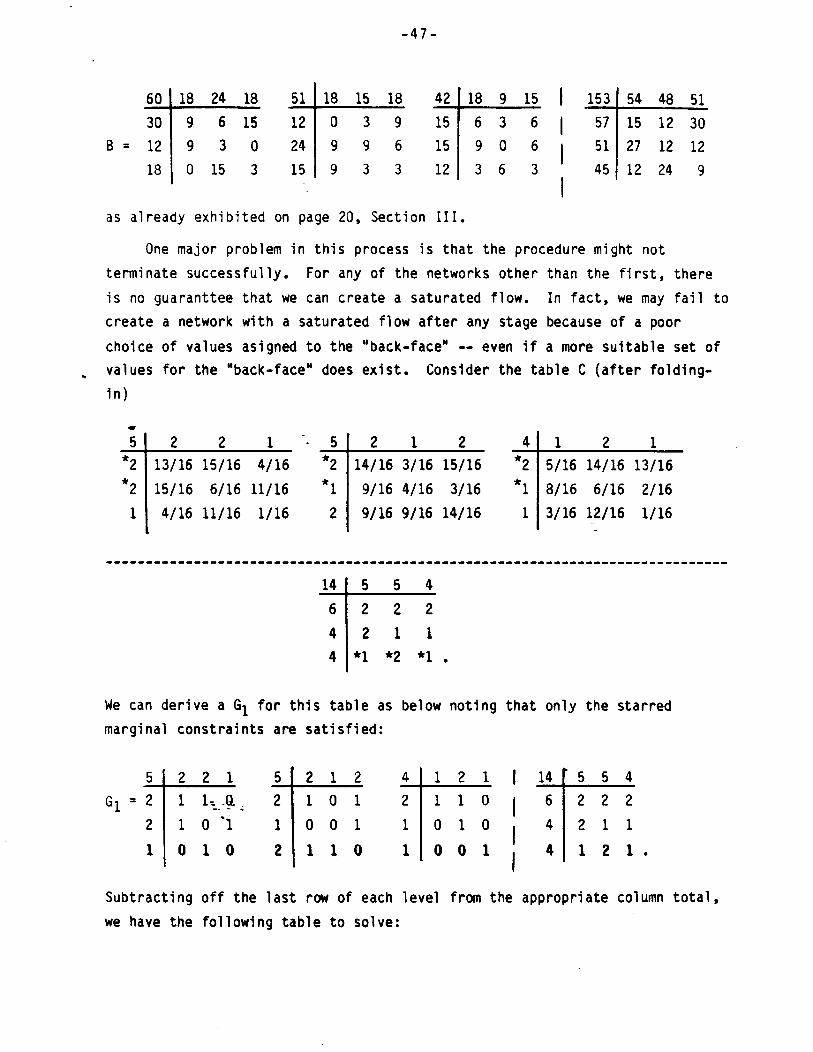
as already exhibited on page 20, Section III.

One major problem in this process is that the procedure might not

terminate successfully. For any of the networks other than the first, there

is no guaranttee that we can create a saturated flow. In fact, we may fail to

create a network with a saturated flow after any stage because of a poor

choice of values asigned to the "back-face" -- even if a more suitable set of

. values for the "back-face" does exist. Consider the table C (after folding-

in)

I

------------------------------------------------------------------------------

14 5 5 4

6 2 2 2

t

4 2 1 1

4 *1 *2 *1 .

We can derive a G1 for this table as below noting that only the starred

marginal constraints are satisfied:

Subtracting off the last row of each level from the appropriate column total,

we have the following table to solve:

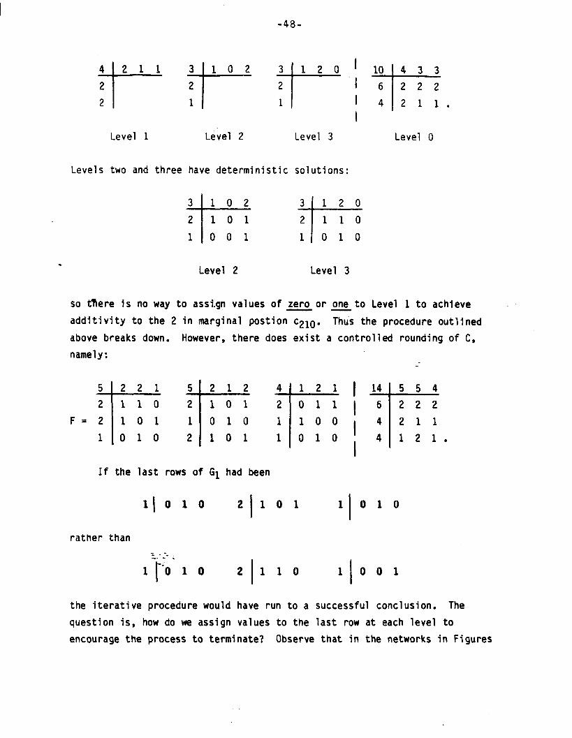
-48-

Level 1 Level 2 Level 3 Level 0

Levels two and three have deterministic solutions:

. Level 2 Level 3

so there is no way to assign values of zero or one to Level 1 to achieve - - additivity to the 2 in marginal postion ~210. Thus the procedure outlined

above breaks down. However, there does exist a controlled rounding of C,

namely:

F=EF-Gi-c.

If the last rows of G1 had been

l(O10 2 I

1 0 1 1 I

0 1 0

rather than

= . -- -. - ;

1 t. ‘0 10 2

I 110 1001

I

the iterative procedure would have run to a successful conclusion. The

question is, how do we assign values to the last row at each level to

encourage the process to terminate? Observe that in the networks in Figures

-49-

3-7, we made no use of costs on arcs. In fact, no objective function was

involved, we only sought a single feasible saturated flow.

According to a result of Gale (1957 ), given marginals of a two-way table

for which there does exist a zero-one assignment for the interior cells, one

can fill up the table, one row at a time, by placing ones in the columns with

the largest residual totals. We cannot apply this rule directly because

addi tivi ty to the marginals of the form c+. 150 must also be maintained when

attempting to resolve each two dimensional level. Instead, we assigned costs

to arcs corresponding to the back-face in a manner to encourage assigning ones

to those columns (at each level) having the greatest residual marginal

value. In particular, for those arcs in Figure 4 corresponding to cells on

the back face -- arcs having initial node of the form (i,j,O) and terminal

node of the form (O,j,k) -- the cost was set to -dOjk. All other arcs had the

cost of zero. This cost assignment did encourage convergence.

* Software was developed to implement this procedure and most tables ran to

a successful termi nation. For those tables that did not terminate, we

observed that a number of arcs had the same costs (i.e., there were ties on

the residual column marginals). To address this, a random component was added .- to all costs on the back face. In particular, for arc ((i,j,O), (O,j,k))

corresponding to a vertical shaft in the figures, the cost was set to

-1OOdOjk - r

where r is a random integer between one and fifty. Using this new cost

assignment, if a table did not reach a successful termination, the table was

reset to run from the very beginning at which time alternative random values

are assigned. Under this new regimen, tables did run to a successful

termination in one or more repetitions. In the next section we discuss

extensions to this basic procedure and software developed at the Census Bureau

for three dim&$anal controlled rounding following this strategy, and we

report on performance.

-50.

v. SOFTWARE FOR THREE DIMENSIONAL CONTROLLED ROUNDING

In the previous section we presented the basic methodology underlying a

heuristic for three dimensional controlled rounding. In this section we go

into further details and report on testing results and program performance.

As discussed in Section II and III, beyond seeking an arbitrary

controlled rounding, we can search for controlled roundinys which are weakly

zero-restricted or better yet zero-restricted. To that end, we set up three

programs for controlled rounding: program ZR to find zero-restricted

controlled roundings, program WZR to find weakly zero-restricted controlled

roundings (some of which may be zero-restricted), and program NZR which will

find a controlled rounding that is not necessarily weakly zero-restricted.

Under the program ZR, we set up the network as in Figure 4, however, all

arc: corresponding to cells that are multiples of the base in A are treated in

a special manner. These cells will appear in C as zero corresponding to an

interior cell of A or second order marginal (aiO0, aOj0, aDOk) and they will

appear as one corresponding to an integer first order marginal (aojk, aiOk, or aij0) or third order marginal (aOO0). Arcs corresponding to a zero cell in C

are forced to have a zero flow (in fact, they are removed from the network)

while arcs corresponding to a one in C are forced to have a flow of one. The

cost along each remaining back face arc (as discussed earlier) is:

where r is a random integer between 1 and 50. Arcs not on the back face have

cost zero. This cost assignment is to assist program termination by

encouraging a to be placed in a column with the greatest residual

"demand", as in the sense of Gale (1957).

The next,program, -. -- . WZR, has its network as in Figure 4, however all arcs

corresponding to true zeros on the even order marginals are forced to have a

zero flow (regarding an interior cell as a O-order marginal) and all arcs

corresponding to true zeros on the odd order marginals are forced to have a

flow of one unit. Arcs corresponding to non-zero multiples of the base in A

have no corresponding restriction (in contrast to program ZR). Although we do

allow these arcs to have a flow of one for even order marginals and zero for

-51.

the odd order marginals so that corresponding non-zero multiple of the base b

can be increased in A, one generally would like to discourage such behavior.

Accordingly, the cost for an arc on the back-face in WZR is:

aijk('OO)z~~-2)n-100dOjk- r,

where

0 if a

'ijk = ijk

is not a multiple of the base

,, if a..

JJk is a non-zero multiple of the base

and

n is the order of a cell,

r is a random integer between 1 and 50.

That is, n=O for an interior cell and n = 1, 2, or 3 for a first, second, or

third order marginal respectively. Since a first or third order marginal

which is a multiple of the base does not change when the corresponding arc is

set to one, we encourage these arcs be set to one by giving them a smaller

cost. An interior value or second order marginal which is a multiple of the

base does not change when the corresponding arc is set to zero so we encourage

these arcs to be set to zero by giving them a relatively higher cost.

Combining these observations, the factor (-1)" is a part of the cost

expression. Since we would prefer to increase an integer which is an interior

cell rather than a first order marginal, a first order marginal rather than a

second order marginal, and so on, the factor (2)" is included in the cost

function.

Although the assignment of zero-one on the non-back-face positions is

wiped clean after each iteration, one would prefer not to set an arc

corresponding'ghn even order non-back-face non-zero multiple of a base

position to one or set an arc corresponding to an odd order non-back-face non-

zero multiple of the base to zero. The reason for this is one may be led down

the path that will force such an interior position to be set to one (or zero)

when it reaches the back-face. To discourage this behavior, the non-back-face

arcs corresponding to a non-zero multiple of the base in A are given the cost:

-520

aj jk( loo)2(-2)ns

Even though costs on the back-face dominate, setting costs on the non-back-

face help direct the program to solutions which tend not to change non-zero

multiples of the base. .-

The final program is call NZR, and in this program the network includes

all arcs shown in Figure 4. Zero cells in A can be increased to the value of

the base and non-zero multiples of the base can be increased by the value of

the base. In order to avoid such changes to the extent possible, costs on

arcs are set as follows. The cost for the arc corresponding to Cell cijk is:

on back-face .

aijk(loo)2(-2)n - 100dOjk- r

on non-back-face

“jjk( 1oo)2(02)n

where

0

"W = 1

10,000

if a ijk

is not a multiple of the base

if a.. Uk

is a non-zero multiple of the base

if aijk = 0

and

n is the order of a cell, r is a random integer between 1 and 50.

The rationale for this costing is an extension of the arguments provided above

for WZR. Note that the cost function above can be viewed as a single cost

function which.ac.comnodates all programs: ZR, WZR, and NZR. We are

experimenting with variations on this cost function for added program

efficiency.

A single main program has been set up which takes a three dimensional

table as input, attempts to round employing up to a fixed number of

repetitions of ZR, followed by up to a fixed number of repetitions of WZR,

-530

followed by up to a fixed number of iterations of NZR. If a controlled

rounding was not found after repetitions of NZR the table is printed out for

examination and analysis. As will be discussed more below, virtually all

tables were resolved within ZR. In the body of the main program, after a

table is read in, the derived table C is constructed following along the lines

in Section III and a sequence of network is defined following the lines in

Section IV. Software for solving a network flow problem is called as a

subroutine to solve the sequence of networks using the unified cost function,

and the results of the sequence of saturated flows is interpreted as the

solution of the controlled rounding as in Section V.

The network flow software, called Minimum Cost Flow (MCF), was developed

at the University of Texas, see (Glover and Klingman 1982). After reading in

an RxCxL table, the dimensions are reordered if necessary so that R is less

thy C and L. Since R equals the number of back-faces that must be "pulled-

off" in reducing the table size (the next iteration will be on an (R-1)xCxL

table) it was reasonable to expect that this ordering of dimensions would

reduce the running time of the program because fewer iterations would be

required. After running a variety of tables, this was very clearly seen to be

the case.

.

We have tested this program and report here on a family of simulations to

impart the flavor of program performance. These tests were executed on a

SPERRY 8600, 1180 series at the Census Bureau. All CPU time in the tables

below are given in terms of 1108 CPU equivelants. (Actual 1180 run times are

about one-third the CPU times displayed).

For the tests we report on below, five sets of 2x2x5 tables were randomly

generated, each set having 1,000 tables. The sets were generated to contain:

0% 25% 50% 75% and 90%

: - --

zero cells. The three subroutines discussed above were linked; however,

all 5,000 tables successful zero-restricted controlled roundings were found in

ZR (the first of the linked programs). Since that was the case, we severed

the linked programs and tested the same randomly generated tables under ZR,

WZR, and NZR independently. In the next three tables we display the results

of this testing.

-54.

PROCEDURE ZR --- TABLE SIZE 2x2x5

Percent zeros 0% 25% 50% 75% 90%

Number of Tables 1000 1000 1000 1000 1000

Number remaining after: one iteration 153 229 196 119 five iterations 17 27 31 32 ten-iterations 3 5 5 4 fifteen iterations 0 0 2 1

Most repititions needed for a single table

13 15 16 16 18

Time in CPU seconds 96/210 93/215 731194 481162 (MCF Time)/(Total Time)

. including IO and diagnostic information

TABLE 1 a

PROCEDURE WZR -- TABLE SIZE 2x2x5

Percent zeros 0%

Number of tables 1000

Number remaining after one repitition 1 five repititions 0 ten repititions 0 fifteen repitions 0

Most repititions needed 2 for a single table

Time in CPU seconds (MCF Time)/(Total Time)

104/201

including IO and diagnostic information

Number of multiples of base increased

160

Number of tables in which a multiple of base was increased

149

25% 50% 75% 90%

1000 1000 1000 1oob

26 44 27 6 1

% 4 0

0 0 0 0 0 x

7 6 7 5

971195 891189 741173 611157

13 5 3 1

251122

268 245 133 20

206 184 103 15

TABLE 2

-55.

PROCEDURE NZR -- TABLE SIZE 2x2x5

.

Percent zeros 0% 25%

Number of tables 1000 1000

Number remaining after one repitition 1 3 five repititions 0 0 ten repititions 0 0 fifteen repititions 0 0

Most repititions needed 2 4 for a single table

Time in CPU seconds 104/199 99/194 (MCF Time)/(Total Time) including IO and diagnostic information

Number of multiples 160 295 ol+base increased _.

Number of Tables in which multiples of base was increased

149 233 241 133 22

Number of zeros increased to one

0 51

Number of tables in which true zero increased to one

0 46 83 60 14

TABLE 3

All information in these tables should be regarded as

50%

1000

75%

1000

90%

1000

921187 86/ 181 791174

345 205 38

108 101 -25

several runnings of these same tables with different seeds for the random

approximate. In

number generator, the number of repetitions, number of zeros changed, and so

on, varied considerably. The objective in presenting these tables is to

impart a broad sense of how these programs performed.

= . -- -. - * -.

-56.

In the process of evaluating this heuristic, we observed that the cost

function employed was not alriays giving a result desired. Consider the

following 2x2x2 table, A, for which we seek a base 3 controlled rounding:

For a base 3 weakly zero-restricted controlled rounding, F of C, we must have

at least:

Using the cost function as described above and the starred constraints,

the last row at each level must look like:

12 3 3 6 2 3 0 0 3 = . ;

- F = t 3 -0 3

6 0 3 3 3

yielding the unique

-57-

12 3 3 6

F = t 3 00 3

3 3 0 0

6 0 3 3

9 3 3 3

3 0 0 3

t

3 0 3 0

3 3 0 0

From which we obtain the controlled rounding

. This rounding is weakly zero-restricted but not zero-restricted. In fact, no

zero-restricted controlled rounding could be found for this table using the

prggram ZR under the cost function described above because the last row was

forced. However, a base'-3 zero-restricted rounding, B of A, does exist,

namely:

The problem is that the cost function above based in part on residual column

totals does not allow finding such a solution. To remedy this problem, in

addition to the cost strategy described earlier, we also assign costs which do

not take the residual column totals into consideration. Recall that for each

of the programs ZR, WZR and NZR the cost functions above could have been

expressed in a unified manner:

back face = . -- -. - ; -.

aijk('00)2(-2)n-Ioodojk-r

non-back face

-58-

where r, aijk, dOjk and n are defined earlier. The contribution of column

total residuals is the term

-1OOdOj k 9

which when removed yields costs:

back face

non-back face

The cost strategy when running any of the programs, ZR, WZR or NZR is as

follows. Allow for at most five repititions of the program for a given table

under the first cost function above (which includes the residual column totals

term), and if the program fails to obtain a controlled rounding then begin

using the second cost function (which does not include the residual column

totals term) for subsequent repetitions. Benefit of this modification to the

cost function showed up when running larger tables than reported on above.

We now summarize findings on program performance for somewhat larger

tables. As one would expect larger tables took longer to run and required

more repetitions before yielding a controlled rounding. The number of overall

iterations was reduced by using the combi nation of cost functions as described

above rather than using only the cost functions with column residual totals.

Using the linked program as discussed earlier, we obtained controlled

roundings for all but two 2x8~10 tables in ZR and all but eleven 4x6x8 tables

in ZR; they a%:$elded controlled roundings in WZR. In the tables below we

display results from running 500 2x8~10 and 500 4x6x8 randomly generated

tables.

.

-59-

PROGRAM ZR-WZR-NZR LINKED -- TABLE SIZE 2x8~10

Percent zeros 0%

Number of tables 100

Number remaining after one repitition 14 twenty-five repititions 0 fifty repititions one hundred repititions

Most repititions needed 4 for a single table

Time in CPU seconds 64/110 (MCF Time)/(Total Time) including IO and diagnostic information

Number of multiples 0 of base increased -.

Number of Tables in which multiples of base was increased

0

Number of zeros increased to one

0

Number of tables in which true zero increased to one

0

25% 50% 75% 90%

100 100 100 100

59 74 7 16 3 11 1 1

100 ZR 100 ZR 1 WZR 27 WZR

235/ 387 4081707

73 43 5 0 2 0 0 0

56 14

1441309 26194

26 6 0 0

1 0 0

0

0

0 -- 0

0 0

TABLE 4

z - -- -- - ;

*.

-6O-

PROGRAM ZR-WZR-NZR LINKED -- TABLE SIZE 4x6x8

.

Percent zeros 0% 25% 50% 75% 90%

Number of tables 100 100 100 100 100

Number remaining after one repitition 36 71 92 91 47 twenty-five repititions 0 25 27 18 0 fifty repititions one hundred repititions 00 :

14 5 : 0”

Most repititions needed 12 100 ZR 100 ZR 70 25 for a single table 3 WZR 43 WZR

Time in CPU seconds 146/221 6201899. 99711525 400/720 561157 (MCF Time)/(Total Time) including IO and diagnostic information

Number of multiples Uf base increased -0

Number of Tables in which multiples of base was increased

Number of zeros increased to one

Number of tables in which true zero increased to one

As noted earlier, all information in these tables should be regarded as

0 17 56 0 0

0 1 ‘5 0 0

0 0 0 0 -- 0

0 0 0 0 0

TABLE 5

approximate. In several runnings of these same tables with different seeds . for the random number generator, the number of repetitions, number of zeros

changed, and so on, varied considerably. As earlier, the objective in

presenting these tables is to impart a broad sense of how these procedures

perform. :.-I- ; -.

-61-

VI. ALTERNATIVE PROCEDURE FOR CONTROLLED ROUNDING

In an earlier report, (Greenberg, 1988), we describe an alternative

procedure for controlled rounding of two dimensional tables in which a non-

zero multiple of the base can either increase or decrease. We outline this

procedure here and show how it is applied to three dimensional tables.

If A is an RxCxL table, we say the RxCxL table B is a controlled roundinq

base b if

. Ibijkwaijk 1 5 b for i=l,... ,R j=l,...,C k-l s**-s L.

The rounding is said to be zero-restricted if

I

and is weakly zero-restricted if

IbijkMaijkl'b if aijk>o

bijk'O if aijk=O .

Every controlled rounding under the old definition is a controlled rounding

(resp., weakly zero-restricted, zero-restricted controlled rounding) under the

new definition, however the converse is not true. Returning to the first

example by Ernst (page 23), E,

3011 T; 3 1 0 1 1 3 1 1 0 1 3 1 1 1 0

000 0 0 10 0 l/2 l/2 1 0 l/2 0 l/2 1 0 l/2 l/2 0

1 0 l/2 0 l/2 0 0 0 0 0 1 l/2 0 0 l/2 1 l/2 l/2 0 0

1 0 0 l/2 l/2 1 l/2 0 0 l/2 0 0 0 0 0 1 l/2 0 l/2 0

1 0 l/2 l/2 0 1 l/2 0 l/2 0 1 l/2 l/2 0 0 0 0 0 0 0

-62-

The following table, H2, is a controlled rounding of E under the new

definition but not the old definition:

--------------------r---r--------------------------------------------------------

11 3 3 2 3

3 0111

I

3 1 1 0 1

2 1 0 1 0

3 110 1.

The composite table

as discussed in Section V had no controlled rounding under the standard

definition, however it does have a controlled rounding under the new

definition, nwly, -.

B=

-63-

where H1 is the interior of the controlled rounding of E displayed in Section

V (page 23) and Ii2 is the interior of the controlled rounding of E displayed

above.

The example, E3 (page 29), formed by adding l/300 to all cells of E2

(page 25), which failed to have a controlled rounding under the old definition

also fails to have a controlled rounding under the new definition. In fact,

if a table has no cells which are a multiple of the base, the two procedures

for controlled rounding (new and old) are identical.

In (Greenberg, 1988) we show how to set up a network flow problem for

controlled rounding of two dimensional tables under the new definition.

Basically, corresponding to each cell which is a non-zero multiple of the base

w there are two arcs in the network formulation rather than one. Costs are

assigned arcs to encourage a non-zero multiple of the base not change in

obtaining a controlled rounding; and it is equally "costly" to decrease a non-

zero multiple of the base-(by the base value) as it is to increase a non-zero

multiple of the base. For zero-restricted controlled roundings to two

definitions are the same. For two dimensional controlled rounding algorithms

and software to extend the usual definition of controlled rounding to obtain

roundings corresponding to the new definition are explicitly described.

The same modifications applied to procedures presented here for three

dimension controlled rounding allow the development of algorithms and software

to obtain three dimensional controlled roundings corresponding to the new

definition. We omit the details here, however, they can easily be carried

though by referring to the earlier report. We developed computer programs for

three dimensional controlled rounding under the new definition and report

below on performance.

Since every controlled rounding under the new definition is also a

controlled rounding under the old definition, we expected the new technique to

be more effici+-t-in finding non-zero-restricted controlled roundings. In

particular, for--higher dimensional tables we hoped that under the new

procedures fewer repetitions would be needed to resolve a problem table. We

also hoped that tables failing to have a controlled rounding under the old

definition would have controlled roundings under the new definition. As it

turns out, the average number of repetitions needed for finding non-zero-

restricted controlled roundings when running a family of randomly generated

-64-

higher dimensional tables (2x8~10 and 4x6~8) under the new definition was

indeed somewhat lower than under the old definition. However, since more arcs

are required under the new definition (two per cell for non-zero multiples of

the base) the overall time for program performance increased. The increase

offset any savings due to fewer repetitions, and program performance for the

new procedure was less efficient than for the old.

As noted above, there exist examples of tables having controlled

roundings under the new definition but not under the old. But the examples

were rather contrived, and we saw no instances of this phenomenon when

examining randomly generated tables or tables arising from actual 1980

Decennial Census tabulations. For all the reasons above, we did not pursue

extensive program development of the new method of controlled rounding for m

three dimensional tables, but rather kept the original ZR-WZR-NZR linked

programs as our basic three dimension controlled rounding software. I

VII. SUMMARY

In this report we exhibit an effective and efficient heuristic procedure

for three dimensional controlled rounding. We discuss factors motivating this

heuristic and provide examples of program performance and program

limitations. Under extensive, testing software developed for this methodology

has performed extremely well based on randomly generated tables and tabulation

arrays taken from the 1980 Decennial Censuses.

These procedures were developed at the Bureau of the Census within the

framework of Disclosure Avoidance research for the 1990 Decennial Censuses.

One option for the public release of standard tabulation files which will

maintain the confidentiality of respondents is to round all table values. The

application of controlled rounding within the setting of disclosure avoidance

is discussed in considerable detail in (Greenberg, 1986). Software based on

the methods presented in this report was extensively tested and evaluated on

standard tabul'kion files taken from the 1980 Decennial Census. Based on these

tests, it was determined that if controlled rounding would be the disclosure

avoidance methodology used on the 1990 Decennial Census standard tabulation

files, this software would be an effective and efficient vehicle for three

dimensional controlled rounding implementation.

-65-

REFERENCES

Cox, Lawrence H. (1987), "A Constructive Procedure for Unbiased Controlled

Rounding*, Journal of the American Statistical Society, 82, 50-524.

and Ernst, Lawrence R. (1982), "Controlled Rounding",

INFOR, 20, 423-432. Reprinted in Some Recent Advances in the Theory,

Computation, and Application of Network Flow Models, University of

Toronto Press, 1983, pp. 139-148.

Fagan, James T., Greenberg, Brian V., Hemnig, Robert .

(1986), "Research at the Census Bureau into Disclosure Avoidance

Techniques for Tabular Data', Proceedings of the Section on Survey

*Research Methods, American Statistical Association, pp. 388-393.

Ernst, Lawrence (1987), Private Communication.

Gale, David (1957), "A Theorem on Flows in Networks", Pacific:Journal of

Mathematics, 7, 1073-1082.

(1960), The Theory of Li,near Economic Models, McGraw

Hill, New York.

Glover, Fred and Klingman, Darwin (1982), "Recent Developments in Computer

Implementation Technology for Network Flow Algorithms", INFOR, 20, 433-

452.

Gondron, Michel and Minoux, Michel (1984), Graphs and Algorithms, John Wiley

and Sons, New York. = . -- -. - i

Greenberg, Briai V. (1986), "Designing a Disclosure Avoidance Methodology for

the 1990 Decennial Censuses", presented at 1990 Census Data Products Fall

Conference, Arlington, Virginia.

-66-

(1988) 9 "An Alternative Formulation of Controlled

Rounding", Statistical Research Division Report Series, Census/SRD/RR-

88/01, Bureau of the Census, Statistical Research Division, Washington,

D.C.

2 - -- -. - .

-.