Embed Size (px)
Citation preview

Control-Theoretic Data Smoothing
Biswadip DeyP. S. Krishnaprasad
Department of Electrical and Computer Engineering&
Institute for Systems ResearchUniversity of Maryland, College Park
Maryland, USA
53rd IEEE Conference on Decision and Control - 2014Los Angeles, California, USA
December 17, 2014
B. Dey, P. S. Krishnaprasad Control-Theoretic Data Smoothing CDC’14 - 12/17/2014 1 / 18

Background and Motivation
Objective: Given a time series of noisy data, reconstruct/generate a path in the underlying space which traversesthrough the data points.
Curve ReconstructionQuantum Information Processing (Quantum State Traversal) Brody et al., PRL 2012
Computer Vision (Curve Completion) Ben-Yosef et al., PAMI 2012
Issues: This inverse problem is ill-posed.Non-uniqueHigh sensitivity to noise
Our Approach: Regularized InversionIntroduce a generative model to treat the data points as output from an underlying dynamical system.Impose regularization by adding a penalty term to fit error.
B. Dey, P. S. Krishnaprasad Control-Theoretic Data Smoothing CDC’14 - 12/17/2014 2 / 18

Background and Motivation
B. Dey, P. S. Krishnaprasad Control-Theoretic Data Smoothing CDC’14 - 12/17/2014 3 / 18

Outline
1 Data Smoothing in a Euclidean Setting (Rn)Maximum PrincipleSketch of ProofExample Problem
2 Data Smoothing in Matrix Lie-Group Setting (G)Maximum PrincipleSketch of ProofLie-Poisson ReductionExample Problem
3 Conclusion
B. Dey, P. S. Krishnaprasad Control-Theoretic Data Smoothing CDC’14 - 12/17/2014 4 / 18

Data Smoothing in a Euclidean Setting (Rn)
1 Data Smoothing in a Euclidean Setting (Rn)Maximum PrincipleSketch of ProofExample Problem
2 Data Smoothing in Matrix Lie-Group Setting (G)Maximum PrincipleSketch of ProofLie-Poisson ReductionExample Problem
3 Conclusion
B. Dey, P. S. Krishnaprasad Control-Theoretic Data Smoothing CDC’14 - 12/17/2014 5 / 18
Data Smoothing in a Euclidean Setting (Rn) Maximum Principle
Maximum Principle for Data Smoothing on Rn
Data Smoothing as a Regularized Inversion
Minimizeq(t0);u
J(q(t0), u
)=
tN∫t0
L(t, q(t), u(t)
)dt+
N∑i=0
Fi(q(ti)
)subject to: q(t) = f
(t, q(t), u(t)
), q : [t0, tN ]→ Rn, u ∈ U =
{u : [t0, tN ]→ U
} (1)
PMP for data smoothing (Theorem 2.2)
Let u∗ be an optimal control input for (1), and q∗ denote the corresponding state trajectory. Then, by defining apre-Hamiltonian as H(t, q, p, u) = 〈p, f(t, q, u)〉 − L(t, q, u), we can show that there exists a costate trajectoryp : [t0, tN ]→ Rn such that
q∗(t) =∂H
∂p
(t, q∗(t), p(t), u∗(t)
), p(t) = −
∂H
∂q
(t, q∗(t), p(t), u∗(t)
), (2)
and, H(t, q∗, p, u∗) = maxu∈U
H(t, q∗, p, u), (3)
at the points of continuity. Moreover, the penalties on intermediate state yield jump discontinuities given by
p(t+i )− p(t−i ) =∂Fi
(q(ti)
)∂q(ti)
, i = 0, 1, . . . , N. (4)
Also, boundary values of the costate variables satisfyp(t−0 ) = p(t+N ) = 0. (5)
B. Dey, P. S. Krishnaprasad Control-Theoretic Data Smoothing CDC’14 - 12/17/2014 6 / 18

Data Smoothing in a Euclidean Setting (Rn) Sketch of Proof
Highlights of The Proof
We introduce a new state variable: q : [t0, tN ]→ R.
y(t) ,
(q(t)q(t)
)∈ Rn+1 =⇒ y(t) =
(L(t, q(t), u(t)
)f(t, q(t), u(t)
) )︸ ︷︷ ︸,g(t,y(t),u(t)
), y(t+i )− y(t−i ) =
(Fi(q(ti)
)0
)
This transforms the problem into the Mayer form, as J(q(t0), u
)= q(t+N ) = J
(y(t0), u
).
Perturbed Control (Needle Variation):
uw,I(t) ,
{u∗(t) if t /∈ Iw if t ∈ I , w ∈ U, I = (b− εa, b] ⊂ (t0, tN ), a > 0
Construct the perturbed trajectory, and compute the perturbation in the terminal state y(t+N ).
Construct the terminal cone at y∗(t+N ), through concatenation of needle variations.
B. Dey, P. S. Krishnaprasad Control-Theoretic Data Smoothing CDC’14 - 12/17/2014 7 / 18

Data Smoothing in a Euclidean Setting (Rn) Example Problem
Example Problem: Trajectory Reconstruction1
Trajectory Reconstruction
Minimizeq(t0),u
J(q(t0), u
)=
N∑i=0
‖r(ti)− ri‖2 + λ
tN∫t0
uT (t)u(t)dt
subject to q(t) = Aq(t) +Bu(t), r(t) = Cq(t)
q(t0) ∈ R9, u ∈ U
(6)
A =
0 I3 00 0 I30 0 0
B =
00I3
C =
[I3 0 0
]
L(t, q, u) = λuTu
Fi(q(ti)
)= q(ti)C
TCq(ti)− 2q(ti)CT ri + rTi ri
Optimal Control Input
u∗(t) =1
2λBT p(t)
State-costate Dynamicsd
dt
[q∗(t)p(t)
]=
[A 1
2λBBT
0 −AT] [
q∗(t)p(t)
]Boundary Values and Jump Conditions
p(t−0 ) = p(t+N ) = 0
p(t+i )− p(t−i ) = 2CT[Cq(ti)− ri
]
1B. Dey, P. S. Krishnaprasad, “Trajectory Smoothing as a Linear Optimal Control Problem”, 50th Annual Allerton Conf., pp. 1490 - 1497, Oct’2012.
B. Dey, P. S. Krishnaprasad Control-Theoretic Data Smoothing CDC’14 - 12/17/2014 8 / 18

Data Smoothing in a Euclidean Setting (Rn) Example Problem
Example Problem: Trajectory Reconstruction1
Trajectory Reconstruction
Minimizeq(t0),u
J(q(t0), u
)=
N∑i=0
‖r(ti)− ri‖2 + λ
tN∫t0
uT (t)u(t)dt
subject to q(t) = Aq(t) +Bu(t), r(t) = Cq(t)
q(t0) ∈ R9, u ∈ U
(6)
A =
0 I3 00 0 I30 0 0
B =
00I3
C =
[I3 0 0
]L(t, q, u) = λuTu
Fi(q(ti)
)= q(ti)C
TCq(ti)− 2q(ti)CT ri + rTi ri
Optimal Control Input
u∗(t) =1
2λBT p(t)
State-costate Dynamicsd
dt
[q∗(t)p(t)
]=
[A 1
2λBBT
0 −AT] [
q∗(t)p(t)
]Boundary Values and Jump Conditions
p(t−0 ) = p(t+N ) = 0
p(t+i )− p(t−i ) = 2CT[Cq(ti)− ri
]1B. Dey, P. S. Krishnaprasad, “Trajectory Smoothing as a Linear Optimal Control Problem”, 50th Annual Allerton Conf., pp. 1490 - 1497, Oct’2012.
B. Dey, P. S. Krishnaprasad Control-Theoretic Data Smoothing CDC’14 - 12/17/2014 8 / 18
Data Smoothing in Matrix Lie-Group Setting (G)
1 Data Smoothing in a Euclidean Setting (Rn)Maximum PrincipleSketch of ProofExample Problem
2 Data Smoothing in Matrix Lie-Group Setting (G)Maximum PrincipleSketch of ProofLie-Poisson ReductionExample Problem
3 Conclusion
B. Dey, P. S. Krishnaprasad Control-Theoretic Data Smoothing CDC’14 - 12/17/2014 9 / 18
Data Smoothing in Matrix Lie-Group Setting (G) Maximum Principle
Maximum Principle for Data Smoothing in a Matrix Lie-Group Setting
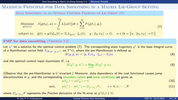
Data Smoothing as an Optimal Control Problem on Lie Group (G)
Minimizeg(t0);u
J(g(t0), u
)=
tN∫t0
L(u(t)
)dt+
N∑i=0
F(g(ti), gi
)subject to: g(t) = g(t)ξu(t) = TeLg(t) · ξu(t), g : [t0, tN ]→ G, u ∈ U =
{u : [t0, tN ]→ U
} (7)
PMP for data smoothing (Theorem 3.2)
Let u∗ be a solution for the optimal control problem (7). The corresponding state trajectory g∗ is the base integral curveof a Hamiltonian vector field XH(g∗,p,u∗) on T ∗G, where the pre-Hamiltonian is defined as
H(g, p, u) = 〈p, TeLg · ξu〉 − L(u) (8)
and the optimal control input maximizes H, i.e.H(g∗, p, u∗) = Max
u∈UH(g∗, p, u). (9)
(Observe that the pre-Hamiltonian is G invariant.) Moreover, data dependency of the cost functional causes jumpdiscontinuities in p, and the corresponding boundary values and jump conditions are given as
p(t−0 ) = p(t+N ) = 0 (10)
and, p(t+i )− p(t−i ) = Dg∗(ti)F , i = 0, 1, · · · , N (11)
where Dg∗(ti)F represents the Frechet derivative of the fit-error at g∗(ti) ∈ G.
B. Dey, P. S. Krishnaprasad Control-Theoretic Data Smoothing CDC’14 - 12/17/2014 10 / 18
Data Smoothing in Matrix Lie-Group Setting (G) Sketch of Proof
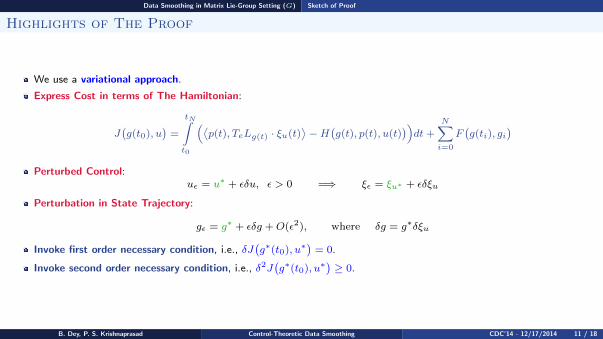
Highlights of The Proof
We use a variational approach.
Express Cost in terms of The Hamiltonian:
J(g(t0), u
)=
tN∫t0
(⟨p(t), TeLg(t) · ξu(t)
⟩−H
(g(t), p(t), u(t)
))dt+
N∑i=0
F(g(ti), gi
)Perturbed Control:
uε = u∗ + εδu, ε > 0 =⇒ ξε = ξu∗ + εδξu
Perturbation in State Trajectory:
gε = g∗ + εδg +O(ε2), where δg = g∗δξu
Invoke first order necessary condition, i.e., δJ(g∗(t0), u∗
)= 0.
Invoke second order necessary condition, i.e., δ2J(g∗(t0), u∗
)≥ 0.
B. Dey, P. S. Krishnaprasad Control-Theoretic Data Smoothing CDC’14 - 12/17/2014 11 / 18

Data Smoothing in Matrix Lie-Group Setting (G) Lie-Poisson Reduction
A Quick Review of Lie-Poisson Reduction
Poincare 1-form:
Θa(ξ′(0)
)=⟨π(ξ(0)
), Tπ(a)Lπ(a)−1 ·
(Taπ · ξ′(0)
)⟩Define a Hamiltonian vector field on T ∗G(H•), by exploiting the symplectic formassociated with the Poincare 1-form(ω = −dΘ).
Poisson Bracket:
φ, ψ 7→ {φ, ψ} = ω(Hφ,Hψ)
• φ, ψ are smooth (C∞) functions on T ∗G
Lie-Poisson Bracket:
π∗{h1, h2}g∗ = {h1, h2}g∗◦π = {π∗h1, π∗h2}
• π∗: Pullback by π• h1, h2 are smooth (C∞) functions on g∗
B. Dey, P. S. Krishnaprasad Control-Theoretic Data Smoothing CDC’14 - 12/17/2014 12 / 18
Data Smoothing in Matrix Lie-Group Setting (G) Example Problem
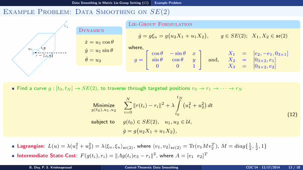
Example Problem: Data Smoothing on SE(2)
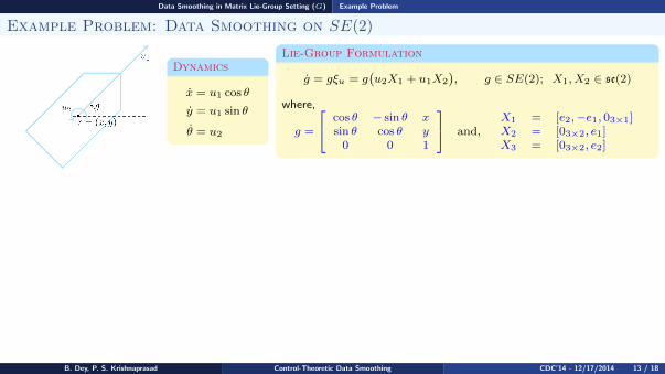
Dynamics
x = u1 cos θ
y = u1 sin θ
θ = u2
Lie-Group Formulation
g = gξu = g(u2X1 + u1X2
), g ∈ SE(2); X1, X2 ∈ se(2)
where,
g =
cos θ − sin θ xsin θ cos θ y
0 0 1
and,X1 = [e2,−e1, 03×1]X2 = [03×2, e1]X3 = [03×2, e2]
Find a curve g : [t0, tN ]→ SE(2), to traverse through targeted positions r0 → r1 → · · · → rN
Minimizeg(t0),u1,u2
N∑i=0
‖r(ti)− ri‖2 + λ
tN∫t0
(u21 + u22
)dt
subject to g(t0) ∈ SE(2), u1, u2 ∈ U ,g = g
(u2X1 + u1X2
),
(12)
Lagrangian: L(u) = λ(u21 + u22) = λ〈ξu, ξu〉se(2), where 〈v1, v2〉se(2) = Tr(v1MvT2 ), M = diag{ 12, 12, 1}
Intermediate State-Cost: F (g(ti), ri) = ‖Ag(ti)e3 − ri‖2, where A = [e1 e2]T
B. Dey, P. S. Krishnaprasad Control-Theoretic Data Smoothing CDC’14 - 12/17/2014 13 / 18
Data Smoothing in Matrix Lie-Group Setting (G) Example Problem
Example Problem: Data Smoothing on SE(2)
Dynamics
x = u1 cos θ
y = u1 sin θ
θ = u2
Lie-Group Formulation
g = gξu = g(u2X1 + u1X2
), g ∈ SE(2); X1, X2 ∈ se(2)
where,
g =
cos θ − sin θ xsin θ cos θ y
0 0 1
and,X1 = [e2,−e1, 03×1]X2 = [03×2, e1]X3 = [03×2, e2]
Find a curve g : [t0, tN ]→ SE(2), to traverse through targeted positions r0 → r1 → · · · → rN
Minimizeg(t0),u1,u2
N∑i=0
‖r(ti)− ri‖2 + λ
tN∫t0
(u21 + u22
)dt
subject to g(t0) ∈ SE(2), u1, u2 ∈ U ,g = g
(u2X1 + u1X2
),
(12)
Lagrangian: L(u) = λ(u21 + u22) = λ〈ξu, ξu〉se(2), where 〈v1, v2〉se(2) = Tr(v1MvT2 ), M = diag{ 12, 12, 1}
Intermediate State-Cost: F (g(ti), ri) = ‖Ag(ti)e3 − ri‖2, where A = [e1 e2]T
B. Dey, P. S. Krishnaprasad Control-Theoretic Data Smoothing CDC’14 - 12/17/2014 13 / 18

Data Smoothing in Matrix Lie-Group Setting (G) Example Problem
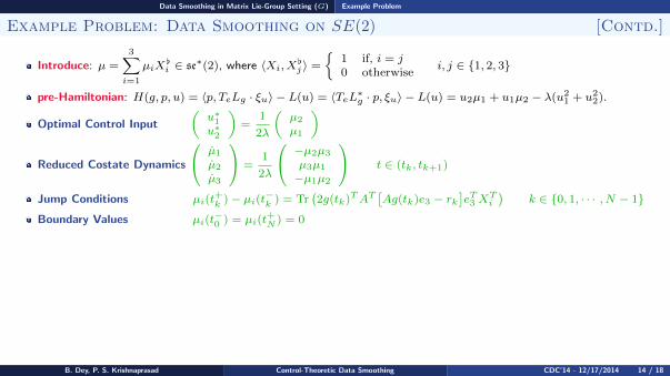
Example Problem: Data Smoothing on SE(2) [Contd.]
Introduce: µ =3∑i=1
µiX[i ∈ se∗(2), where 〈Xi, X[
j 〉 =
{1 if, i = j0 otherwise
i, j ∈ {1, 2, 3}
pre-Hamiltonian: H(g, p, u) = 〈p, TeLg · ξu〉 − L(u) = 〈TeL∗g · p, ξu〉 − L(u) = u2µ1 + u1µ2 − λ(u21 + u22).
Optimal Control Input
(u∗1u∗2
)=
1
2λ
(µ2µ1
)
Reduced Costate Dynamics
µ1µ2µ3
=1
2λ
−µ2µ3µ3µ1−µ1µ2
t ∈ (tk, tk+1)
Jump Conditions µi(t+k )− µi(t−k ) = Tr
(2g(tk)TAT
[Ag(tk)e3 − rk
]eT3 X
Ti
)k ∈ {0, 1, · · · , N − 1}
Boundary Values µi(t−0 ) = µi(t
+N ) = 0
Conserved Quantities
{Hamiltonian: h = 1
4λ(µ21 + µ22)
Casimir: C = 14λ
(µ22 + µ23
)
Closed-form Solution
µ1(t) = ±2
√λh Cn
(√Cλ
(t+ φk),√
hC
)µ2(t) = 2
√λh Sn
(√Cλ
(t+ φk),√
hC
)t ∈ (tk, tk+1)
µ3(t) = ±2√λC Dn
(√Cλ
(t+ φk),√
hC
)
B. Dey, P. S. Krishnaprasad Control-Theoretic Data Smoothing CDC’14 - 12/17/2014 14 / 18
Data Smoothing in Matrix Lie-Group Setting (G) Example Problem
Example Problem: Data Smoothing on SE(2) [Contd.]
Introduce: µ =3∑i=1
µiX[i ∈ se∗(2), where 〈Xi, X[
j 〉 =
{1 if, i = j0 otherwise
i, j ∈ {1, 2, 3}
pre-Hamiltonian: H(g, p, u) = 〈p, TeLg · ξu〉 − L(u) = 〈TeL∗g · p, ξu〉 − L(u) = u2µ1 + u1µ2 − λ(u21 + u22).
Optimal Control Input
(u∗1u∗2
)=
1
2λ
(µ2µ1
)
Reduced Costate Dynamics
µ1µ2µ3
=1
2λ
−µ2µ3µ3µ1−µ1µ2
t ∈ (tk, tk+1)
Jump Conditions µi(t+k )− µi(t−k ) = Tr
(2g(tk)TAT
[Ag(tk)e3 − rk
]eT3 X
Ti
)k ∈ {0, 1, · · · , N − 1}
Boundary Values µi(t−0 ) = µi(t
+N ) = 0
Conserved Quantities
{Hamiltonian: h = 1
4λ(µ21 + µ22)
Casimir: C = 14λ
(µ22 + µ23
)
Closed-form Solution
µ1(t) = ±2
√λh Cn
(√Cλ
(t+ φk),√
hC
)µ2(t) = 2
√λh Sn
(√Cλ
(t+ φk),√
hC
)t ∈ (tk, tk+1)
µ3(t) = ±2√λC Dn
(√Cλ
(t+ φk),√
hC
)
B. Dey, P. S. Krishnaprasad Control-Theoretic Data Smoothing CDC’14 - 12/17/2014 14 / 18

Data Smoothing in Matrix Lie-Group Setting (G) Example Problem
Example Problem: Data Smoothing on SE(2) [Contd.]
Introduce: µ =3∑i=1
µiX[i ∈ se∗(2), where 〈Xi, X[
j 〉 =
{1 if, i = j0 otherwise
i, j ∈ {1, 2, 3}
pre-Hamiltonian: H(g, p, u) = 〈p, TeLg · ξu〉 − L(u) = 〈TeL∗g · p, ξu〉 − L(u) = u2µ1 + u1µ2 − λ(u21 + u22).
Optimal Control Input
(u∗1u∗2
)=
1
2λ
(µ2µ1
)
Reduced Costate Dynamics
µ1µ2µ3
=1
2λ
−µ2µ3µ3µ1−µ1µ2
t ∈ (tk, tk+1)
Jump Conditions µi(t+k )− µi(t−k ) = Tr
(2g(tk)TAT
[Ag(tk)e3 − rk
]eT3 X
Ti
)k ∈ {0, 1, · · · , N − 1}
Boundary Values µi(t−0 ) = µi(t
+N ) = 0
Conserved Quantities
{Hamiltonian: h = 1
4λ(µ21 + µ22)
Casimir: C = 14λ
(µ22 + µ23
)
Closed-form Solution
µ1(t) = ±2
√λh Cn
(√Cλ
(t+ φk),√
hC
)µ2(t) = 2
√λh Sn
(√Cλ
(t+ φk),√
hC
)t ∈ (tk, tk+1)
µ3(t) = ±2√λC Dn
(√Cλ
(t+ φk),√
hC
)B. Dey, P. S. Krishnaprasad Control-Theoretic Data Smoothing CDC’14 - 12/17/2014 14 / 18
Conclusion
1 Data Smoothing in a Euclidean Setting (Rn)Maximum PrincipleSketch of ProofExample Problem
2 Data Smoothing in Matrix Lie-Group Setting (G)Maximum PrincipleSketch of ProofLie-Poisson ReductionExample Problem
3 Conclusion
B. Dey, P. S. Krishnaprasad Control-Theoretic Data Smoothing CDC’14 - 12/17/2014 15 / 18

Conclusion
Conclusion
SummaryDeveloped an extended version of the maximum principle to address data smoothing using generative models.Results are applicable to problems in both Euclidean and finite dimensional matrix Lie group settings.This approach yields solution in a semi-analytical way.
Future DirectionsTo consider Lagrangians involving higher derivatives of control input.
B. Dey, P. S. Krishnaprasad Control-Theoretic Data Smoothing CDC’14 - 12/17/2014 16 / 18

References
References
B. Dey and P. S. Krishnaprasad, “Control-Theoretic Data Smoothing”, Proc. 53rd IEEE Conference on Decision andControl, pp. 5064-5070, Los Angeles, CA, 2014.
B. Dey and P. S. Krishnaprasad, “Trajectory Smoothing as a Linear Optimal Control Problem”, Proc. 50th AnnualAllerton Conference on Communication, Control, and Computing, pp. 1490-1497, Allerton, IL, 2012.
E. Justh and P. S. Krishnaprasad, “Optimal Natural Frames”, Communications in Information and Systems,11(1):17-34, 2011.
P. S. Krishnaprasad, “Lie-Poisson structures, dual-spin spacecraft and asymptotic stability”, Nonlinear Analysis:Theory, Methods and Applications, 9(10):1011-1035, 1985.
P. S. Krishnaprasad, “Optimal control and Poisson reduction”, Tech. Rep. TR 93-87, Institute for Systems Research,University of Maryland, College Park, MD, 1993.
H. Sussmann and J. Willems, “300 years of optimal control: from the brachystochrone to the maximum principle”,IEEE Control Systems, 17(3):32-44, 1997.
D. Liberzon, Calculus of Variations and Optimal Control Theory: A Concise Introduction, Princeton, NJ: PrincetonUniversity Press, 2011.
G. B. Yosef and O. B. Shahar, “A tangent bundle theory for visual curve compeltion”, IEEE Trans. on PatternAnalysis and Machine Intelligence, 34(7):1263-1280, 2012.
D. C. Brody, D. D. Holm and D. M. Meier, “Quantum Splines”, Physical Review Letter, 109(10):100501, 2012.
B. Dey, P. S. Krishnaprasad Control-Theoretic Data Smoothing CDC’14 - 12/17/2014 17 / 18

Thank You !!!
B. Dey, P. S. Krishnaprasad Control-Theoretic Data Smoothing CDC’14 - 12/17/2014 18 / 18