Embed Size (px)
Citation preview

Control Systems ILecture 9: Analysis of Feedback Systems 2: the Nyquist condition
Readings: Guzzella, Chapter 8.1-3
Emilio Frazzoli
Institute for Dynamic Systems and ControlD-MAVT
ETH Zurich
November 11, 2016
E. Frazzoli (ETH) Lecture 9: Control Systems I 11/11/2016 1 / 31
Tentative schedule
# Date Topic Chapter
1 Sept. 23 Introduction, Signals and Systems 12 Sept. 30 Modeling, Linearization 2, 3
3 Oct. 7 Analysis 1: Time response, Stability 44 Oct. 14 Analysis 2: Diagonalization, Modal Coordinates 5.1, 5.4-5.55 Oct. 21 Transfer functions 1: Definition and properties 66 Oct. 28 Transfer functions 2: Poles and Zeros 77 Nov. 4 Introduction to Feedback: internal stability,
root locus5.2-3, 9.1-3, 13.3
8 Nov. 11 Frequency response 89 Nov. 18 Analysis of feedback systems 2: the Nyquist
condition9.4-6
10 Nov. 25 Specifications for feedback systems 1011 Dec. 2 Feedback control synthesis 1 1112 Dec. 9 Feedback control synthesis 1, continued 1113 Dec. 16 Feedback control synthesis 2 1214 Dec. 23 Implementation issues 14
E. Frazzoli (ETH) Lecture 9: Control Systems I 11/11/2016 2 / 31

E. Frazzoli (ETH) Lecture 9: Control Systems I 11/11/2016 3 / 31

Examples
ks+1
s2+s+1
r y
−
Re
Im
E. Frazzoli (ETH) Lecture 9: Control Systems I 11/11/2016 4 / 31

Examples
k1
(s+1)(s2+s+1)r y
−
Re
Im
E. Frazzoli (ETH) Lecture 9: Control Systems I 11/11/2016 5 / 31
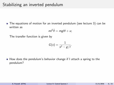
Stabilizing an inverted pendulum
The equations of motion for an inverted pendulum (see lecture 3) can bewritten as
ml2θ = mglθ + u;
The transfer function is given by
G (s) =1
s2 − g/l.
How does the pendulum’s behavior change if I attach a spring to thependulum?
E. Frazzoli (ETH) Lecture 9: Control Systems I 11/11/2016 6 / 31

Proportional control of an inverted pendulum
k1
s2−g/lr y
−
Re
Im
E. Frazzoli (ETH) Lecture 9: Control Systems I 11/11/2016 7 / 31

Proportional-derivative control of an inverted pendulum
kp + kd s1
s2−g/lr y
−
Re
Im
E. Frazzoli (ETH) Lecture 9: Control Systems I 11/11/2016 8 / 31

Root locus summary (for now)
Great tool for back-of-the-envelope control design, quick check forclosed-loop stability.
Qualitative sketches are typically enough. There are many detailed rules fordrawing the root locus in a very precise way: if you really need to do that,just use matlab or other methods.
Closed-loop poles start from the open loop poles, and are “repelled” by them.
Closed-loop poles are “attracted” by zeros (or go to infinity). Here you seean obvious explanation why non-minimum-phase zeros are in general to beavoided.
Remember that the root locus must be symmetric wrt the real axis.
E. Frazzoli (ETH) Lecture 9: Control Systems I 11/11/2016 9 / 31

Classical methods for feedback control
Remember: the main objective is to assess/design the properties of theclosed-loop system by exploiting the knowledge of the open-loop system, andavoiding complex calculations. We have three main methods:Root Locus
Quick assessment of control design feasibility. The insights are correct andclear.Can only be used for finite-dimensional systems (e.g. systems with a finitenumber of poles/zeros)Difficult to do sophisticated design.Hard to represent uncertainty.
Nyquist plotThe most authoritative closed-loop stability test. It can always be used (finiteor infinite-dimensional systems)Easy to represent uncertainty.Difficult to draw and to use for sophisticated design.
Bode plotsPotentially misleading results unless the system is open-loop stable andminimum-phase.Easy to represent uncertainty.Easy to draw, this is the tool of choice for sophisticated design.
E. Frazzoli (ETH) Lecture 9: Control Systems I 11/11/2016 10 / 31
Frequency response
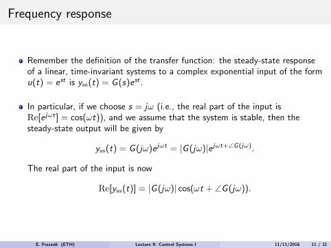
Remember the definition of the transfer function: the steady-state responseof a linear, time-invariant systems to a complex exponential input of the formu(t) = est is yss(t) = G (s)est .
In particular, if we choose s = jω (i.e., the real part of the input isRe[e jωt ] = cos(ωt)), and we assume that the system is stable, then thesteady-state output will be given by
yss(t) = G (jω)e jωt = |G (jω)|e jωt+∠G(jω).
The real part of the input is now
Re[yss(t)] = |G (jω)| cos(ωt + ∠G (jω)).
E. Frazzoli (ETH) Lecture 9: Control Systems I 11/11/2016 11 / 31

Frequency response
In other words, the steady-state response to a sinusoidal input of frequency ωis a sinusoidal output of the same frequency such that:
1 the amplitude of the output is |G(jω)| times the amplitude of the input;2 the phase of the output lags the phase of the input by ∠G(jω)|.
0 5 10 15 20 25 30-1
-0.8
-0.6
-0.4
-0.2
0
0.2
0.4
0.6
0.8
1Linear Simulation Results
Time (seconds)
Ampl
itude
E. Frazzoli (ETH) Lecture 9: Control Systems I 11/11/2016 12 / 31
How can we display/visualize the frequency response?
E. Frazzoli (ETH) Lecture 9: Control Systems I 11/11/2016 13 / 31

Frequency response plots
The frequency response G (jω) ∈ C is a complex function of a single realargument ω ∈ R.
We basically have two options to plot the frequency response:
1 A parametric curve showing G(jω) in the complex plane, in which ω isimplicit. This leads to the polar plot and eventually to the Nyquist plot.
2 Two separate plots for, e.g., real and imaginary part of G(jω) or — better —the magnitude and phase of G(jω) as a function of ω. The latter choice leadsto the Bode plot.
E. Frazzoli (ETH) Lecture 9: Control Systems I 11/11/2016 14 / 31

The Bode Plot
The Bode plot is actually composed of two plot: the magnitude and thephase plots.
On the horizontal axis of both plots, we report the frequency ω on alogarithmic scale (base 10).
On the vertical axis we report1 The logarithm of G(jω) (in base 10), or, equivalently, in dB (deciBels). Note
that we use the convention that
|G(jω)|[dB] = 20 log10 |G(jω)|.
Note that “one decade” = 20 dB.2 The phase ∠G(jω). Usually given in degrees (ok to use radians though).
Note: Since magnitudes multiply (i.e., their logs add) and phases add, thesechoices of vertical coordinates makes it possible to just add Bode plots ofserial connections.
Also, inverting the transfer function is equivalent to reflection about thehorizontal axis, in both Bode plots.
E. Frazzoli (ETH) Lecture 9: Control Systems I 11/11/2016 15 / 31
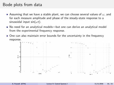
Bode plots from data
Assuming that we have a stable plant, we can choose several values of ω, andfor each measure amplitude and phase of the steady-state response to asinusoidal input sin(ωt).
No need for an analytical models—but one can derive an analytical modelfrom the experimental frequency response.
One can also maintain error bounds for the uncertainty in the frequencyresponse.
E. Frazzoli (ETH) Lecture 9: Control Systems I 11/11/2016 16 / 31
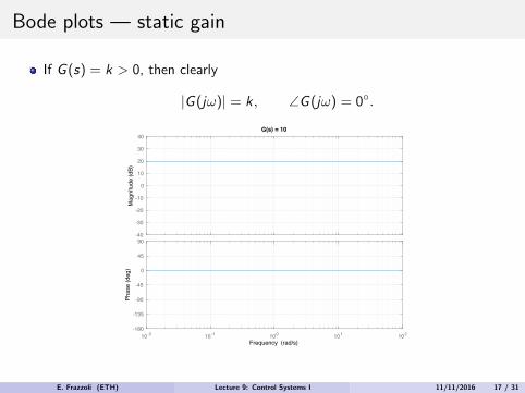
Bode plots — static gain
If G (s) = k > 0, then clearly
|G (jω)| = k , ∠G (jω) = 0◦.
-40
-30
-20
-10
0
10
20
30
40M
agni
tude
(dB)
10-2 10-1 100 101 102-180
-135
-90
-45
0
45
90
Phas
e (d
eg)
G(s) = 10
Frequency (rad/s)
E. Frazzoli (ETH) Lecture 9: Control Systems I 11/11/2016 17 / 31

Bode plots — Integrator
The frequency response of G (s) = 1/s is simply G (jω) = 1jω = −j 1ω , hence
|G (jω)| =1
ω, ∠G (jω) = −90◦.
Re
Im
jω
E. Frazzoli (ETH) Lecture 9: Control Systems I 11/11/2016 18 / 31
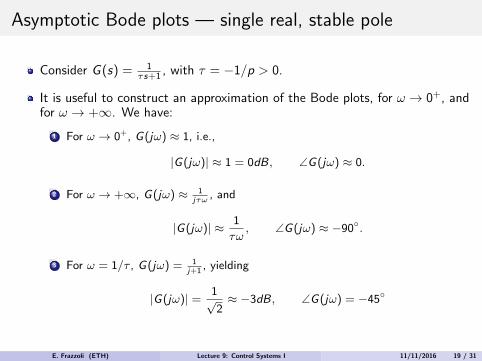
Asymptotic Bode plots — single real, stable pole
Consider G (s) = 1τs+1 , with τ = −1/p > 0.
It is useful to construct an approximation of the Bode plots, for ω → 0+, andfor ω → +∞. We have:
1 For ω → 0+, G(jω) ≈ 1, i.e.,
|G(jω)| ≈ 1 = 0dB, ∠G(jω) ≈ 0.
2 For ω → +∞, G(jω) ≈ 1jτω
, and
|G(jω)| ≈ 1
τω, ∠G(jω) ≈ −90◦.
3 For ω = 1/τ , G(jω) = 1j+1
, yielding
|G(jω)| =1√2≈ −3dB, ∠G(jω) = −45◦
E. Frazzoli (ETH) Lecture 9: Control Systems I 11/11/2016 19 / 31

Asymptotic Bode plots — single real, stable pole
Re
Im
jω
E. Frazzoli (ETH) Lecture 9: Control Systems I 11/11/2016 20 / 31
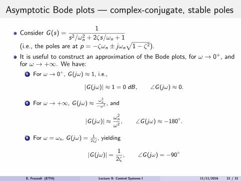
Asymptotic Bode plots — complex-conjugate, stable poles
Consider G (s) =1
s2/ω2n + 2ζs/ωn + 1
(i.e., the poles are at p = −ζωn ± jωn
√1− ζ2).
It is useful to construct an approximation of the Bode plots, for ω → 0+, andfor ω → +∞. We have:
1 For ω → 0+, G(jω) ≈ 1, i.e.,
|G(jω)| ≈ 1 = 0 dB, ∠G(jω) ≈ 0.
2 For ω → +∞, G(jω) ≈ ω2n
−ω2 , and
|G(jω)| ≈ ω2n
ω2, ∠G(jω) ≈ −180◦.
3 For ω = ωn, G(jω) = 12ζj
, yielding
|G(jω)| =1
2ζ, ∠G(jω) = −90◦
E. Frazzoli (ETH) Lecture 9: Control Systems I 11/11/2016 21 / 31

Asymptotic Bode plots — complex-conjugate, stable poles
Re
Im
jωjω
E. Frazzoli (ETH) Lecture 9: Control Systems I 11/11/2016 22 / 31
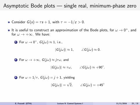
Asymptotic Bode plots — single real, minimum-phase zero
Consider G (s) = τs + 1, with τ = −1/z > 0.
It is useful to construct an approximation of the Bode plots, for ω → 0+, andfor ω → +∞. We have:
1 For ω → 0+, G(jω) ≈ 1, i.e.,
|G(jω)| ≈ 1, ∠G(jω) ≈ 0.
2 For ω → +∞, G(jω) ≈ jτω, and
|G(jω)| ≈ τω, ∠G(jω) ≈ +90◦.
3 For ω = 1/τ , G(jω) = j + 1, yielding
|G(jω)| =√
2, ∠G(jω) = +45◦
E. Frazzoli (ETH) Lecture 9: Control Systems I 11/11/2016 23 / 31

Asymptotic Bode plots — single real, minimum-phase zero
Re
Im
jω
The Bode plots for 1/G (s) can be obtained by “flipping” the Bode plots for G (s)about the horizontal (frequency) axis. Can you draw the Bode plots for adifferentiator, for complex-conjugate minimum-phase zeros, etc.?
E. Frazzoli (ETH) Lecture 9: Control Systems I 11/11/2016 24 / 31

Asymptotic Bode plots — single real, non-minimum-phasezero
Consider G (s) = −τs + 1, with τ = 1/z > 0.
It is useful to construct an approximation of the Bode plots, for ω → 0+, andfor ω → +∞. We have:
1 For ω → 0+, G(jω) ≈ 1, i.e.,
|G(jω)| ≈ 1 = 0 dB, ∠G(jω) ≈ 0.
2 For ω → +∞, G(jω) ≈ −jτω, and
|G(jω)| ≈ τω, ∠G(jω) ≈ −90◦.
3 For ω = 1/τ , G(jω) = −j + 1, yielding
|G(jω)| =√
2, ∠G(jω) = −45◦
E. Frazzoli (ETH) Lecture 9: Control Systems I 11/11/2016 25 / 31

Asymptotic Bode plots — single real, non-minimum-phasezero
The phase plot for a non-minimum-phase zero is the same as that for a stablepole.
Re
Im
jω
E. Frazzoli (ETH) Lecture 9: Control Systems I 11/11/2016 26 / 31
Putting it all together: Bode plots for complicated transfer functions
E. Frazzoli (ETH) Lecture 9: Control Systems I 11/11/2016 27 / 31
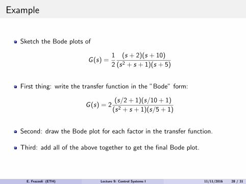
Example
Sketch the Bode plots of
G (s) =1
2
(s + 2)(s + 10)
(s2 + s + 1)(s + 5)
First thing: write the transfer function in the ”Bode” form:
G (s) = 2(s/2 + 1)(s/10 + 1)
(s2 + s + 1)(s/5 + 1)
Second: draw the Bode plot for each factor in the transfer function.
Third: add all of the above together to get the final Bode plot.
E. Frazzoli (ETH) Lecture 9: Control Systems I 11/11/2016 28 / 31
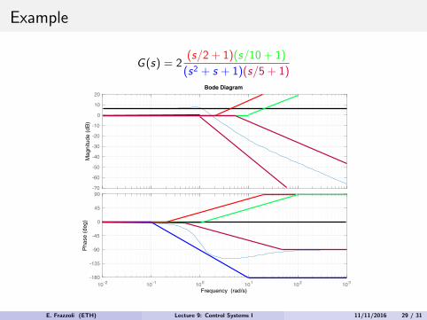
Example
G (s) = 2(s/2 + 1)(s/10 + 1)
(s2 + s + 1)(s/5 + 1)
-70
-60
-50
-40
-30
-20
-10
0
10
20M
agni
tude
(dB)
10-2 10-1 100 101 102 103-180
-135
-90
-45
0
45
90
Phas
e (d
eg)
Bode Diagram
Frequency (rad/s)
E. Frazzoli (ETH) Lecture 9: Control Systems I 11/11/2016 29 / 31

Example
G (s) = 2(s/2 + 1)(s/10 + 1)
(s2 + s + 1)(s/5 + 1)
-70
-60
-50
-40
-30
-20
-10
0
10
20
Mag
nitu
de (d
B)
10-2 10-1 100 101 102 103-180
-135
-90
-45
0
45
90
Phas
e (d
eg)
Bode Diagram
Frequency (rad/s)
E. Frazzoli (ETH) Lecture 9: Control Systems I 11/11/2016 30 / 31
Bode’s Law
In the Bode plot, the magnitude slope and the phase are not independent.
In particular, if the slope of the Bode magnitude plot is κ db/decade over arange of more than ≈ 1 decade, the phase in that range will be approximatelyκ · 90◦.
E. Frazzoli (ETH) Lecture 9: Control Systems I 11/11/2016 31 / 31