Embed Size (px)
Citation preview

DEPT. of ECE, ATMECE, MYSURU 1
Control Systems
(15EC43)
Department of Electronics and Communication
ATME College of Engineering, Mysuru.

DEPT. of ECE, ATMECE, MYSURU 2
INDEX
1.1 Objectives ......................................................................................................................................... 6
1.2 Introduction ....................................................................................................................................... 6
1.3 Types of control systems: ................................................................................................................. 8
1.4 Block Diagrammatic Representation .............................................................................................. 12
1.4.2 Advantages of Block Diagram Representation: ......................................................................................14
1.5 Block diagram reduction technique ................................................................................................ 14
1.5.1 Block diagram rules .................................................................................................................................15
1.6 Applications of the control systems ................................................................................................ 16
1.7 Feed back Control System .............................................................................................................. 17
1.9 Properties of Systems ...................................................................................................................... 19
1.10 Transfer Function .......................................................................................................................... 19
1.11 Signal Flow Graphs (SFG)............................................................................................................ 21
1.12 Masons gain formula..................................................................................................................... 23
1.13 Outcomes ...................................................................................................................................... 26
1.14 Recommended Questions .............................................................................................................. 26
2.1 Objectives ....................................................................................................................................... 28
2.2 Introduction ..................................................................................................................................... 28
2.3 Response to a Unit Step Input –First Order .................................................................................... 29
2.4 Response to a Unit Ramp Input ...................................................................................................... 32
2.5 Response to a Unit Step Input - Second Order System .................................................................. 33
2.6 Proportional, Integral and Derivative Controller (PID Control) : ................................................... 36
2.7 Outcomes ........................................................................................................................................ 38
2.8 Recommended questions ................................................................................................................ 38
3.1 Objectives ........................................................................................ Error! Bookmark not defined.
3.2 Introduction ...................................................................................... Error! Bookmark not defined.
3.3 Concept of stability: ......................................................................... Error! Bookmark not defined.

DEPT. of ECE, ATMECE, MYSURU 3

DEPT. of ECE, ATMECE, MYSURU 4

DEPT. of ECE, ATMECE, MYSURU 5
MODULE -1
Introduction to Control Systems, Types of Control Systems, Effect ofFeedback Systems, Different
ial equation of Physical Systems Mechanical systems,Electrical systems, Analogous systems. Block
diagram and signal flow graphs: transfer functions, block diagram algebra and signal flow graph.
Structure
1.1 Objectives 6
1.2 Introduction 6
1.3 Types of control systems: 8
1.4 Block Diagrammatic Representation 12
1.4.2 Advantages of Block Diagram Representation: 14
1.5 Block diagram reduction technique 14
1.5.1 Block diagram rules 15
1.6 Applications of the control systems 16
1.7 Feed back Control System 17
1.9 Properties of Systems 19
1.10 Transfer Function 19
1.11 Signal Flow Graphs 21
1.12 Masons gain formula 23
1.13 Recommended Questions 26

DEPT. of ECE, ATMECE, MYSURU 6
1.1 Objectives
Students should be able to make measurements of a system and determine a transfer function.
Open loop and closed loop systems and Electrical analogy of physical systems.
Students will know the Block diagram representation Open loop and closed loop systems and
Electrical analogy of physical systems.
Block diagram reduction technique along with Signal Flow graph using the Mason’s formula.
1.2 Introduction
A control system is one which can control any quantity of interest in a machine, mechanism or
other equipment in order to achieve the desired performance or output.(or) A control system is an
interconnection of components connected or related in such a manner as to command, direct, or
regulate itself or another system. For example consider, the driving system of an automobile. Speed
of the automobile is a function of the position of its accelerator. The desired speed can be maintained
(or a desired change in speed can be achieved) by controlling pressure on the accelerator pedal. This
automobile driving system (accelerator, carburetor and engine-vehicle) constitutes a control system.
Control systems find numerous and widespread applications from everyday to extraordinary in
science, industry, and home. Here are a few examples:
(a) Home heating and air-conditioning systems controlled by a thermostat
(b) The cruise (speed) control of an automobile
(c) Manual control
(i) Opening or closing of a window for regulating air temperature or air quality
(ii) Activation of a light switch to regulate the illumination in a room
(iii) Human controlling the speed of an automobile by regulating the gas supply to the engine
(d) Automatic traffic control (signal) system at roadway intersections
(e) Control system which automatically turns on a room lamp at night, and turns it off in Day light
The general block diagram of a control system is shown below..

DEPT. of ECE, ATMECE, MYSURU 7
Fig.1.1. Block diagram of a control system.
The above method of representation of a control system is known as block diagram representation
where in each block represents an element, a plant, mechanism, device etc., whose inner details are
not indicated. Each block has an input and output signal which are linked by a relationship
characterizing the block. It may be noted that the signal flow through the block is unidirectional.
Basic Control System components : The basic control system components are objectives i.e inputs or
actuating signals to the system and the Output signals or controlled variables etc.The control system
will control the outputs in accordance with the input signals. The relation between these components
is shown in the block diagram.
Fig.1.2 Block control system Components
The components of the control system changes as we move from open loop control system to closed
loop control systems. In a closed loop control system, the feedback control network play an important
role in getting the correct output.
The general block diagram of a control system with feedback is shown below. The error detector
compares a signal obtained through feedback elements, which is a function of the output response,
with the reference input. Any difference between these two signals gives an error or actuating signal,
which actuates the control elements. The control elements in turn alter the conditions in the plant in
such a manner as to reduce the original error.
Control System
Input Signals Output Signals

DEPT. of ECE, ATMECE, MYSURU 8
Fig.1.3 .General block diagram of an automatic control system.
1.3 Types of control systems:
There are basically two types of control systems (i) the open loop system and the (ii) closed loop
System. They can both be represented by block diagrams. A block diagram uses blocks to represent
processes, while arrows are used to connect different input, process and output parts.
(a) Open loop Control System: A system which do not possess any feedback network, and
contains only the input and output relationship is known as a open loop control system.
.
Fig.4. Open loop control system
Examples of the open loop control systems are washing machines, light switches, gas ovens, burglar
alarm system etc.The drawback of an open loop control system is that it is incapable of making
automatic adjustments. Even when the magnitude of the output is too big or too small, the system
can’t make the necessary adjustments. For this reason, an open loop control system is not suitable for
use as a complex control system.
(b) Closed loop control system: A closed loop system is one which uses a feed back control
between input and output. A closed loop control system compares the output with the expected
Process Input Output

DEPT. of ECE, ATMECE, MYSURU 9
result or command status, and then it takes appropriate control actions to adjust the input
signal. Therefore, a closed loop system is always equipped with a sensor, which is used to
monitor the output and compare it with the expected result.
Fig.5.Closed Loop Control system
The output signal is fed back to the input to produce a new output. A well-designed feedback system
can often increase the accuracy of the output.
Examples for closed loop systems are air conditioners, refrigerators, automatic rice cookers,
automatic ticketing machines, etc. For example An air conditioner, uses a thermostat to detect the
temperature and control the operation of its electrical parts to keep the room temperature at a preset
constant.
One advantage of using the closed loop control system is that it is able to adjust its output
automatically by feeding the output signal back to the input. When the load changes, the error signals
generated by the system will adjust the output suitably. The limitation of a closed loop control
systems is they are generally more complicated and thus also more expensive to design.
(c) Linear versus Nonlinear Control Systems : Linear feedback control systems are idealized models
fabricated by the analyst purely for the simplicity of analysis and design
When the magnitudes of signals in a control system are limited to ranges in which system components
exhibit linear characteristics (i.e., the principle of superposition applies), the system is essentially
linear.
But when the magnitudes of signals are extended beyond the range of the linear operation, depending
on the severity of the nonlinearity, the system should no longer be considered linear. For instance,
amplifiers used in control systems often exhibit a saturation effect when their input signals become
large; the magnetic field of a motor usually has saturation properties. Other common nonlinear effects

DEPT. of ECE, ATMECE, MYSURU 10
found in control systems are the backlash or dead play between coupled gear members, nonlinear
spring characteristics, nonlinear friction force or torque between moving members, and so on. Quite
often, nonlinear characteristics are intentionally introduced in a control system to improve its
performance or provide more effective control.
Also the analysis of linear systems is easy and lot of mathematical solutions is available for their
simplification.
Nonlinear systems, on the other hand, are usually difficult to treat mathematically, and there are no
general methods available for solving a wide class of nonlinear systems. In practice , first a linear-
system is modeled by neglecting the nonlinearities of the system and the designed controller is then
applied to the nonlinear system model for evaluation or redesign by computer simulation.
Distinguish between Open loop and closed loop control systems
Open Loop System Closed Loop System
1. An open loop system has the ability to
perform accurately, if its calibration is
good. If the calibration is not perfect its
performance will go down.
2. It is easier to build.
3. In general it is more stable as the feed
back is absent .
4. If-non-linearity’s are present , the
system operation is not good.
5. Feedback is absent
Example :
(i) Traffic control system
(ii) Control of furnace for coal
heating
(iii) An Electric washing machine
1. A closed loop system has got the ability
to perform accurately because of the
feedback.
2. It is difficult to build.
3. Less stable Comparatively
4. Even under the presence of non-
linearity’s the system operates better
than open loop system.
5. Feedback is present
Example:
(i) Pressure control system
(ii) Speed control system
(iii) Temperature control system
(d) Time-Invariant control Systems:

DEPT. of ECE, ATMECE, MYSURU 11
When the parameters of a control system do not change with respect to time during the operation of
the system, the system is called a time-invariant system. In practice, most physical systems contain
elements that drift or vary with time. For example, the winding resistance of an electric motor will
vary when the motor is first being excited and its temperature is rising. Another example of a time-
varying system is a guided-missile control system in which the mass of the missile decreases as the
fuel on board is being consumed during flight. Although a time-varying system without nonlinearity
is still a linear system, the analysis and design of this class of systems are usually much more complex
than that of the linear time-invariant systems.
(e) Continuous and Discrete Data Control Systems: A continuous-data system is one in which the
signals at various parts of the system are all functions of the continuous time variable t. The signals in
continuous-data systems may be further classified as ac or dc. In control systems the ac control
system, means that the signals in the system are modulated by some form of modulation scheme. A
dc control system, on the other hand, simply implies that the signals are un-modulated, but they are
still ac signals according to the conventional definition. The schematic diagram of a closed loop dc
control system is shown below. Typical waveforms of the signals in response to a step-function input
are shown in the figure. Typical components of a dc control system are potentiometers, dc amplifiers,
dc motors, dc tachometers, and so on.
Fig 1.6 Block diagram of Continuous and Discrete Data Control Systems
In ac control systems, the signals are modulated i.e the information is transmitted by an ac carrier
signal. Here the output controlled variable behaves similarly to that of the dc system. In this case, the
DEPT. of ECE, ATMECE, MYSURU 12
modulated signals are demodulated by the low-pass characteristics of the ac motor. Ac control
systems are used extensively in aircraft and missile control systems in which noise and disturbance
often create problems. By using modulated ac control systems with carrier frequencies of 400 Hz or
higher, the system will be less susceptible to low-frequency noise. Typical components of an ac
control system are synchros, ac amplifiers, ac motors, gyroscopes, accelerometers etc.
(f) Discrete Data Control System
If the signal is not continuously varying with time but it is in the form of pulses then the control
system is called Discrete Data Control System. If the signal is in the form of pulse data, then the
system is called Sampled Data Control System. Here the information supplied intermittently at
specific instants of time. This has the advantage of Time sharing system. On the other hand, if the
signal is in the form of digital code, the system is called Digital Coded System. Here use of Digital
computers, micro processors or microcontrollers are made use of such systems and are analyzed by
the Z- transform theory.
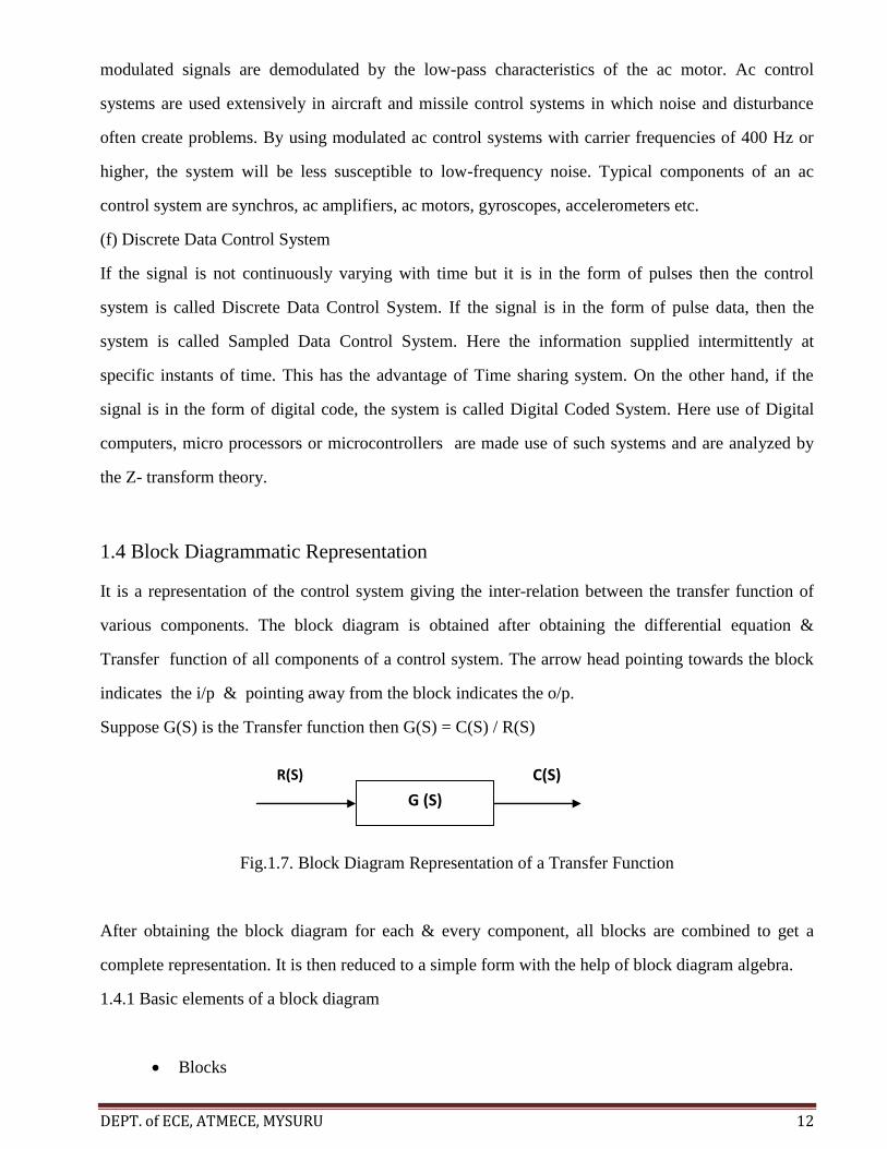
1.4 Block Diagrammatic Representation
It is a representation of the control system giving the inter-relation between the transfer function of
various components. The block diagram is obtained after obtaining the differential equation &
Transfer function of all components of a control system. The arrow head pointing towards the block
indicates the i/p & pointing away from the block indicates the o/p.
Suppose G(S) is the Transfer function then G(S) = C(S) / R(S)
Fig.1.7. Block Diagram Representation of a Transfer Function
After obtaining the block diagram for each & every component, all blocks are combined to get a
complete representation. It is then reduced to a simple form with the help of block diagram algebra.
1.4.1 Basic elements of a block diagram
Blocks
G (S)
R(S) C(S)

DEPT. of ECE, ATMECE, MYSURU 13
Transfer functions of elements inside the blocks
Summing points
Take off points
Arrow
Fig 1.8. Basic elements of a Block Diagram
A control system may consist of a number of components. A block diagram of a system is a pictorial
representation of the functions performed by each component and of the flow of signals. The elements
of a block diagram are block, branch point and summing point.
(a) Block :
In a block diagram all system variables are linked to each other through functional blocks. The
functional block or simply block is a symbol for the mathematical operation on the input signal to the
block that produces the output.
Fig.1.9 Block
(b) Summing point:
The blocks are used to identify many types of mathematical operations, like addition and subtraction
and represented by a circle, called a summing point. As shown below diagram a summing point may
have one or several inputs. Each input has its own appropriate plus or minus sign. A summing point
has only one output and is equal to the algebraic sum of the inputs
BLOCK INPUT
OUTPUT

DEPT. of ECE, ATMECE, MYSURU 14
Fig.1.10 Summing Point
Individual & Overall performance can be studied A takeoff point is used to allow a signal to be used
by more than one block or summing point
(c)Arrow – associated with each branch to indicate the direction of flow of signal
1.4.2 Advantages of Block Diagram Representation:
It is always easy to construct the block diagram even for a complicated system
Function of individual element can be visualized
Over all transfer function can be calculated easily
1.4.3 Limitations of a Block Diagram Representation :
No information can be obtained about the physical construction
Source of energy is not shown
1.5 Block diagram reduction technique
Because of the simplicity and versatility, the block diagrams are often used by control engineers to
describe all types of systems. A block diagram can be used simply to represent the composition and
interconnection of a system. Also, it can be used, together with transfer functions, to represent the
cause-and-effect relationships throughout the system. Transfer Function is defined as the relationship
between an input signal and an output signal to a device.
Procedure to solve Block Diagram Reductions:
Step 1: Reduce the blocks connected in series

DEPT. of ECE, ATMECE, MYSURU 15
Step 2: Reduce the blocks connected in parallel
Step 3: Reduce the minor feedback loops
Step 4: Try to shift take off points towards right and Summing point towards left
Step 5: Repeat steps 1 to 4 till simple form is obtained
Step 6: Obtain the Transfer Function of Overall System
1.5.1 Block diagram rules
(1) Blocks in Cascade [Series]: When two blocks are connected in series , their resultant transfer
function is the product of two individual transfer functions.
(2) Combining blocks in Parallel: When two blocks are connected parallel as shown below ,the
resultant transfer function is equal to the algebraic sum (or difference) of the two transfer
functions.This is shown in the diagram below.
(3) Eliminating a feed back loop: The following diagram shows how to eliminate the feed back loop
in the resultant control system

DEPT. of ECE, ATMECE, MYSURU 16
(4) Moving a take-off point beyond a block: The effect of moving the takeoff point beyond a block is
shown below.
(5) Moving a Take-off point ahead of a block: The effect of moving the takeoff point ahead of a
block is shown below.
1.6 Applications of the control systems
There are various applications of control systems which include biological propulsion; locomotion;
robotics; material handling; biomedical, surgical, and endoscopic ; aeronautics; marine and the
defense and space industries. There are also many household and industrial application examples of
the control systems, such as washing machine, air conditioner, security alarm system and automatic
ticket selling machine, etc.
(i) Washing machine:
The most commonly used house hold application is the washing machine. It comes under automatic
control system ,where the machine automatically starts to pour water, add washing powder, spin and
wash clothes, discharge wastewater, etc. After the completion of all the procedures, the washing
machine will stop the operation.
However, this kind of machine only operates according to the preset time to complete the whole
washing process. It ignores the cleanness of the clothes and does not generate feedback. Therefore,
this kind of washing machine is of open loop control system.

DEPT. of ECE, ATMECE, MYSURU 17
(ii). Air conditioner
The air conditioner is used to automatically control the temperature of the room.In the air conditioner
the coolant circulated in the machine will absorb heat indoor, then it will be transported from the
vaporization device to cooling device. The hot air is then blown to outdoor by a fan. There is an
adjustable temperature device equipped in the air conditioner for the users to adjust the extent of
cooling. When the temperature of the cool air is lower than the preset one, the controller of the air
conditioner will stop the operation of the compressor to cease the circulation of the coolant. The
temperature sensor installed near the vaporization device will continuously measure the indoor
temperature, and send the results to the controller for further processing.This operation will come
under closed loop control system. The simple block diagram of air conditioner system is shown
below.
1.7 Feed back Control System
The feedback control system is represented by the following block diagram .In the diagram feedback
signal is denoted by B(S) and the output is C(S).The input function is denoted by R(S).
The open loop gain of the system is G(S) and the feedback loop gain H(S). Then the feedback
signal b(s) is given by
B(S) = H(S). C(S)
DEPT. of ECE, ATMECE, MYSURU 18
1.8 Transfer function:
The input- output relationship in a linear time invariant system is given by the transfer function. For a
time invariant system it is defined as the ratio of Laplace transform of the out to the Lapalce
transform of the input
The important features of the transfer functions are,
The transfer function of a system is the mathematical model expressing the differential
equation that relates the output to input of the system.
The transfer function is the property of a system independent of magnitude and the nature of
the input .
The transfer function includes the transfer functions of the individual elements. But at the
same time, it does not provide any information regarding physical structure of the system
If the transfer function of the system is known, the output response can be studied for various
types of inputs to understand the nature of the system
It is applicable to Linear Time Invariant system.
It is assumed that initial conditions are zero.
It is independent of i/p excitation.
It is used to obtain systems o/p response.
If the transfer function is unknown, it may be found out experimentally by applying known
inputs to the device and studying the output of the system
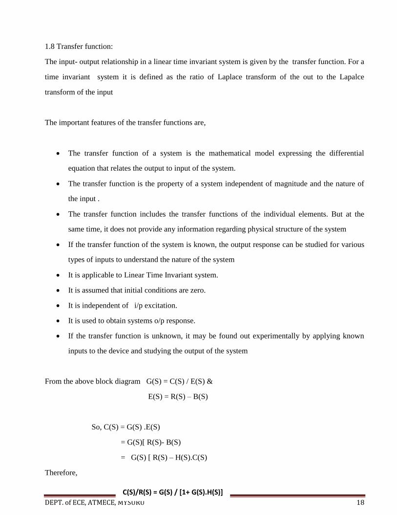
From the above block diagram G(S) = C(S) / E(S) &
E(S) = R(S) – B(S)
So, C(S) = G(S) .E(S)
= G(S)[ R(S)- B(S)
= G(S) [ R(S) – H(S).C(S)
Therefore,
C(S)/R(S) = G(S) / [1+ G(S).H(S)]

DEPT. of ECE, ATMECE, MYSURU 19
This is the transfer function of the closed loop control system
1.9 Properties of Systems
For any control system to understand its performance the following properties are very important.
(i).Linearity: A system is said to be linear if it follows both the law of addtivity and law of
homogeneity. The system which does not follow the law of homogeneity and additively is called a
non-linear system.
If input x1(t) produces response y1(t) and input x2(t) produces response y2(t) then the scaled and
summed input a1x1(t) +b1x2(t) produces the scaled and summed response a1y1(t) +b1y2(t) where a1 and
a2 are real scalars. It follows that this can be extended to an arbitrary number of terms, and so for real
numbers.
(ii) Time Invariance : A system with input x(t) and output y(t) is time-invariant if x(t- t0) is creates
output y ( t – t0) for all inputs x and shifts t0.
(iii) Causality : A system is causal, if the output y(t) at time t is not a function of future inputs and it
depends only on the present and past inputs . All analog systems are causal and all memeoryless
systems are causal.
If the system is causal, then this implies h (t) = 0, t < 0. Alternatively, h[n] =0, n < 0.
(iv) Stability : A system is said to be a stable if for every bounded-input there exists a bounded output
. 1.10 Transfer Function
For a open loop control system shown below the transfer function is the ratio of Laplace transform of
the out-put to the Laplace transform of the input.
G (t) C (t) R (t)

DEPT. of ECE, ATMECE, MYSURU 20
The Laplace transform of the Input is R(S) and the Laplace transform of the output is
C(S) .
So,the Transfer function of the system is G(S) = C(S) / R(S)
Example : Find the transfer function of the following RC circuit
The Laplace transformed Network is shown above. From the circuit we can write that
Vo(S) = 1/ Cs * I(S) & Vi (S ) [ R + 1/Cs ]
Cs * Vo (S) = Vi (S) / [ R + 1/Cs ]
Vo(S )/ Vi (S ) = 1/ { [ R + 1/Cs ]} Cs
Vo(S )/ Vi (S ) = 1/ { [ 1 + RCs ]} = 1/ {
1+ τ s ]} Where τ = RC
Or the Transfer function G (S) = 1/ [1+
τ s]

DEPT. of ECE, ATMECE, MYSURU 21
1.11 Signal Flow Graphs (SFG)
The block diagram method is a useful tool for simplifying the representation of a control system. But
when there are more than two feed back loops and if there exists inter-coupling between feedback
loops, and when a system has more than one input and one output, the block diagram approach is very
complex. Hence an alternate method is proposed by S.J. Mason. This method is called signal flow
graphs. In these graphs each node represents a system variable & each branch connected between two
nodes acts as Signal Multiplier. The direction of signal flow is indicated by an arrow.
A signal flow graph is a diagram that represents a set of simultaneous equations. It consists of a graph
in which nodes are connected by directed branches. The nodes represent each of the system variables.
A branch connected between two nodes acts as a one-way signal multiplier: the direction of signal
flow is indicated by an arrow placed on the branch, and the multiplication factor (transmittance or
transfer function) is indicated by a letter placed near the arrow.
So,in the figure above , the branch transmits the signal x1 from left to right and multiplies it by the
quantity a in the process. The quantity a is the transmittance, or transfer function.
Flow-Graph Definitions : A node performs two functions:
Addition of the signals on all incoming branches and Transmission of the total node signal
(the sum of all incoming signals) to all outgoing
branches
There are three types of nodes .They are Source nodes , Sink nodes and Mixed nodes
Source nodes (independent nodes) : These represent independent variables and have only outgoing
branches. In Fig. 5.21, nodes u and v are source nodes.

DEPT. of ECE, ATMECE, MYSURU 22
Sink nodes (dependent nodes): These represent dependent variables and have only incoming
branches. In Fig (a), nodes x and y are sink nodes.
Mixed nodes (general nodes): These have both incoming and outgoing branches. In Fig. (a), node w
is a mixed node. A mixed node may be treated as a sink node by adding an out going branch of unity
transmittance, as shown in Fig (b), for the equation x = au +bv
and w = cx = cau + cbv
Fig(a) Fig (b)
A path is any connected sequence of branches whose arrows are in the same direction and A
forward path between two nodes is one that follows the arrows of successive branches and in which a
node appears only once. In Fig.(a) the path uwx is a forward path between the nodes u and x.
Flow-Graph Algebra : The following rules are useful for simplifying a signal flow graph:
Series paths (cascade nodes). Series paths can be combined into a single path by multiplying the
transmittances as shown in Fig ( A ).
Path gain. The product of the transmittances in a series path.
Parallel paths. Parallel paths can be combined by adding the transmittances as shown in Fig(B).
Node absorption. A node representing a variable other than a source or sink can be eliminated as
shown in Fig (C).
Feedback loop. Aclosed path that starts at a node and ends at the same node.
Loop gain. The product of the transmittances of a feedback loop.

DEPT. of ECE, ATMECE, MYSURU 23
These results are shown diagrammatically in the following figures (A) ,(B) and C) where the original
diagram and equivalent diagrams are shown.
1.12 Masons gain formula
The relationship between an input variable and an output variable of a signal flow graphis given by
the net gain between input and output nodes and is known as overall gain ofthe system. Masons gain
formula is used to obtain the over all gain (transfer function) of signal flow graphs. According to
Mason’s gain formula Gain is given by
1 11
k
PP
Where, Pk is gain of k th
forward path and Δ is determinant of graph. Here the Δ is given by
Δ = 1-(sum of all individual loop gains)+(sum of gain products of all possible combinations of two
non touching loops –sum of gain products of all possible combination of three non touching loops)
Δk is cofactor of kth
forward path determinant of graph with loops touching k th
forward path. It is
obtained from Δ by removing the loops touching the path Pk.

DEPT. of ECE, ATMECE, MYSURU 24
Finding transfer function from the system flow graphs is explained below by example.
Example1 : Obtain the transfer function of the system whose signal flow graph is shown below.
There are two forward paths: One is Gain of path 1: P1=G1 and the other is Gain of path 2: P2=G2
There are four loops with loop gains:
L1=-G1G3, L2=G1G4, L3= -G2G3, L4= G2G4
There are no non-touching loops.
Δ = 1+G1G3-G1G4+G2G3-G2G4
Forward paths 1 and 2 touch all the loops. Therefore, Δ1= 1, Δ2= 1
So,the transfer function T is given by

DEPT. of ECE, ATMECE, MYSURU 25
Example 2 : Obtain the transfer function of C(s) /R(s) of the system whose signal flow graph shown
below.
From the system flow graph it is clear that
There is one forward path, whose gain is: P1=G1G2G3
There are three loops with loop gains:
L1=-G1G2H1, L2=G2G3H2, L3= -G1G2G3
There are no non-touching loops: Δ = 1-G1G2H1+G2G3H2+G1G2G3
Forward path 1 touches all the loops. Therefore, Δ1= 1.
The transfer function T is given by
( ) 1 1 1 2 3
( ) 1 1 2 1 1 3 2 1 2 3
C S P G G G
R S G G H G G H G G G
System Stability:
The study of stability of a control system is very important to understand the performance . This
means that the system must be stable at all times during operation. Stability may be used to define the
usefulness of the system. Stability studies include absolute & relative stability. Absolute stability is
the quality of stable or unstable performance. Relative Stability is the quantitative study of stability.

DEPT. of ECE, ATMECE, MYSURU 26
The stability study is based on the properties of the Transfer Function. In the analysis, the
characteristic equation is very important ,which describe the transient response of the system. From
the roots of the characteristic equation, following conclusions about the stability can be drawn.
(1) When all the roots of the characteristic equation lie in the left half of the S-plane, the system
response due to initial condition will decrease to zero at time Thus the system will be termed as a
stable system.
(2) When one or more roots lie on the imaginary axis & there are no roots on the RHS of
S-plane, the response will be oscillatory without damping. Such a system will be termed as critically
stable.
(3) When one or more roots lie on the RHS of S-plane, the response will exponentially increase
in magnitude and there by the system will be Unstable.
1.13 Outcomes
Able to design basic structure of control system.
Students will analyze the application of Open loop and closed loop systems.
Students should be able to design basic structure of control system using Block
diagram reduction technique.
Analyze the importance of Signal Flow graph using the Mason’s formula.
1.14 Recommended Questions
1. Name three applications of control systems.
2. Name three reasons for using feedback control systems and at least one reason for not
using them.
3. Give three examples of open- loop systems.
4. Functionally, how do closed – loop systems differ from open loop systems.
5. State one condition under which the error signal of a feedback control system would not
be the difference between the input and output.

DEPT. of ECE, ATMECE, MYSURU 27
6. Name two advantages of having a computer in the loop.
7. Name the three major design criteria for control systems.
8. Name the two parts of a system‘s response.
9. Physically, what happens to a system that is unstable?
10. Instability is attributable to what part of the total response.
11. What mathematical model permits easy interconnection of physical systems?
12. To what classification of systems can the transfer function be best applied?
13. What transformation turns the solution of differential equations into algebraic
manipulations ?
14. Define the transfer function.
15. What assumption is made concerning initial conditions when dealing with transfer
functions?
16. What do we call the mechanical equations written in order to evaluate the transfer
function ?
17. Why do transfer functions for mechanical networks look identical to transfer functions
for electrical network.
Resources:
lpsa.swarthmore.edu/Analogs/ElectricalMechanicalAnalogs.htm
www.newagepublishers.com/samplechapter/001712.pdf
www.youtube.com/watch?v=h_CDoUIYrC0
https://www.scribd.com/doc/7291532/Class-5-6-Analogous-Systems
https://www.google.co.in/?gfe_rd=cr&ei=1r0KVfuYGqHV8gfK-YH4Cg&gws_rd=ssl#
www.dartmouth.edu/~sullivan/22files/System_analogy_all.pdf
MODULE-2
TIME RESPONSE OF FEEDBACK CONTROL SYSTEMS
Standard test signals, Unit step response of the First and Second order Systems. Time
response specifications, steady state errors and error constants. Introduction to PI, PD and PID
controllers.
Structure:

Control Systems 10ES43
DEPT. of ECE, ATMECE, MYSURU 28
2.1 Objectives 28
2.2 Introduction 28
2.3 Response to a Unit Step Input –First Order 29
2.4 Response to a Unit Ramp Input 32
2.5 Response to a Unit Step Input - Second Order System 33
2.6 Proportional, Integral and Derivative Controller (PID Control) : 36
2.7 Outcomes 38
2.8 Recommended questions 38
2.1 Objectives
Get an understanding of the standard test signals
Able to analyze the response of First and second order systems
Understand the different types of steady state errors
2.2 Introduction
(a)Time response analysis
It is an equation or a plot that describes the behavior of a system and gives information about it
with respect to time response specification as overshooting, settling time, peak time, rise time
and steady state error. Time response is formed by the transient response and the steady state
response.
Time response = Transient response + Steady state response.
Transient time response or Natural response describes the behavior of the system in its first short
time until arrives the steady state value. If the input is step function then the output or the
response is called step time response and if the input is ramp, the response is called ramp time
response .. etc.
(b)Transient Response
Control Systems 10ES43
DEPT. of ECE, ATMECE, MYSURU 29
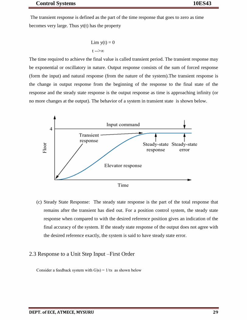
The transient response is defined as the part of the time response that goes to zero as time
becomes very large. Thus yt(t) has the property
Lim y(t) = 0
t -->∞
The time required to achieve the final value is called transient period. The transient response may
be exponential or oscillatory in nature. Output response consists of the sum of forced response
(form the input) and natural response (from the nature of the system).The transient response is
the change in output response from the beginning of the response to the final state of the
response and the steady state response is the output response as time is approaching infinity (or
no more changes at the output). The behavior of a system in transient state is shown below.
(c) Steady State Response: The steady state response is the part of the total response that
remains after the transient has died out. For a position control system, the steady state
response when compared to with the desired reference position gives an indication of the
final accuracy of the system. If the steady state response of the output does not agree with
the desired reference exactly, the system is said to have steady state error.
2.3 Response to a Unit Step Input –First Order
Consider a feedback system with G)s) = 1/τs as shown below

Control Systems 10ES43
DEPT. of ECE, ATMECE, MYSURU 30
The closed loop transfer function of the system is given by
For a unit step input R (s) = 1 / s and the output is given by
Inverse Laplace transformation yields
The plot of c(t) Vs t is shown below
The response is an exponentially increasing function and it approaches a value of unity as

Control Systems 10ES43
DEPT. of ECE, ATMECE, MYSURU 31
t --- > ∞
At t = τ the response reaches a value,
which is 63.2 percent of the steady value. This time, τ is known as the time constant of the
system. One of the important characteristics about the system is its speed of response or how
fast the response is approaching the final value. The time constant τ is indicative of this measure
and the speed of response is inversely proportional to the time constant of the system.Another
important characteristic of the system is the error between the desired value and the actual value
under steady state conditions. This quantity is known as the steady state error of the - system and
is denoted by ess.
The error E(s) for a unity feedback system is given by
For the system under consideration G(s) = 1 / τs and R(s) = 1 /s Therefore
As t ~ ∞ e (t) ~ 0 . Thus the output of the first order system approaches the reference input,
which is the desired output, without any error. In other words, we say a first order system tracks
the step input without any steady state error.
Control Systems 10ES43
DEPT. of ECE, ATMECE, MYSURU 32
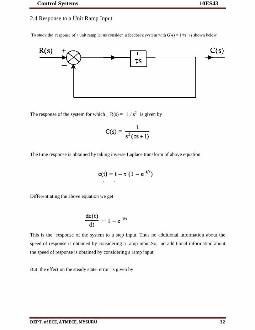
2.4 Response to a Unit Ramp Input
To study the response of a unit ramp let us consider a feedback system with G)s) = 1/τs as shown below
The response of the system for which , R(s) = 1 / s2
is given by
The time response is obtained by taking inverse Laplace transform of above equation
Differentiating the above equation we get
This is the response of the system to a step input. Thus no additional information about the
speed of response is obtained by considering a ramp input.So, no additional information about
the speed of response is obtained by considering a ramp input.
But the effect on the steady state error is given by

Control Systems 10ES43
DEPT. of ECE, ATMECE, MYSURU 33
Thus the steady state error is equal to the time constant of the system. The first order system,
therefore, can not track the ramp input without a finite steady state error. If the time constant is
reduced not only the speed of response increases but also the steady state error for ramp input
decreases. Hence the ramp input is important to the extent that it produces a finite steady state
error.
The response of a first order system for unit ramp input is shown below.
2.5 Response to a Unit Step Input - Second Order System
Let us consider a type 1, second order system as shown in Fig. below. Since G(s) has one pole at
the origin, it is a type one system.

Control Systems 10ES43
DEPT. of ECE, ATMECE, MYSURU 34
The closed loop transfer function is give by,
The transient response of any system depends on the poles of the transfer function T(s). The
roots of the denominator polynomial in s of T(s) are the poles of the transfer function. Thus the
denominator polynomial of T(s), given by
D(s) = τs2 + S + K
is known as the characteristic polynomial of the system and D(s) = 0 is known as the
characteristic equation of the system. The above Eqn. is normally put in standard from, given
by,

Control Systems 10ES43
DEPT. of ECE, ATMECE, MYSURU 35
The poles of T( s), or, the roots of the characteristic equation
S2 + 2δ ωn s + ωn
2 = 0
are given by,
Where is known as the damped natural frequency of the system. If δ > 1,
the two roots s1, s2 are real and we have an over damped system. If δ = 1, the system is known as
a critically damped system. The more common case of δ < 1 is known as the under damped
system.
Steady State Errors : One of the important design specifications for a control system is the
steady state error. The steady state output of any system should be as close to desired output as
possible. If it deviates from this desired output, the performance of the system is not satisfactory
under steady state conditions. The steady state error reflects the accuracy of the system. Among
many reasons for these errors, the most important ones are the type of input, the type of the
system and the nonlinearities present in the system. Since the actual input in a physical system is
often a random signal, the steady state errors are obtained for the standard test signals, namely,
step, ramp and parabolic signals.
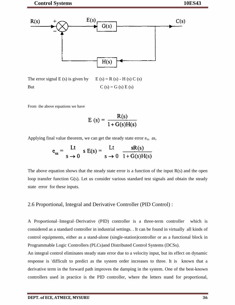
Error Constants : Let us consider a feedback control system as shown below.
Control Systems 10ES43
DEPT. of ECE, ATMECE, MYSURU 36
The error signal E (s) is given by E (s) = R (s) - H (s) C (s)
But C (s) = G (s) E (s)
From the above equations we have
Applying final value theorem, we can get the steady state error ess as,
The above equation shows that the steady state error is a function of the input R(s) and the open
loop transfer function G(s). Let us consider various standard test signals and obtain the steady
state error for these inputs.
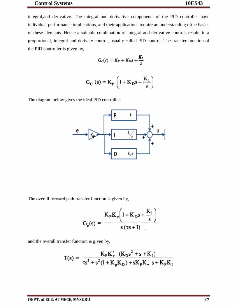
2.6 Proportional, Integral and Derivative Controller (PID Control) :
A Proportional–Integral–Derivative (PID) controller is a three-term controller which is
considered as a standard controller in industrial settings. . It can be found in virtually all kinds of
control equipments, either as a stand-alone (single-station)controller or as a functional block in
Programmable Logic Controllers (PLCs)and Distributed Control Systems (DCSs).
An integral control eliminates steady state error due to a velocity input, but its effect on dynamic
response is 'difficult to predict as the system order increases to three. It is known that a
derivative term in the forward path improves the damping in the system. One of the best-known
controllers used in practice is the PID controller, where the letters stand for proportional,
Control Systems 10ES43
DEPT. of ECE, ATMECE, MYSURU 37
integral,and derivative. The integral and derivative components of the PID controller have
individual performance implications, and their applications require an understanding ofthe basics
of these elements. Hence a suitable combination of integral and derivative controls results in a
proportional, integral and derivate control, usually called PID control. The transfer function of
the PID controller is given by,
The diagram below gives the ideal PID controller.
The overall forward path transfer function is given by,
and the overall transfer function is given by,

Control Systems 10ES43
DEPT. of ECE, ATMECE, MYSURU 38
Proper choice of Kp, KD and Kr results in satisfactory transient and steadystate responses. The
process of choosing proper Kp, KD, at Kr for a given system is known as tuning of a P ID
controller.
2.7 Outcomes
Student will be able to analyze the different test signals and apply it to design the first order and
second order systems.
Understand the effect of different steady state errors as the type and order of the system changes
Able to understand the working of P, PI and PID controllers
2.8 Recommended questions

Control Systems 10ES43
DEPT. of ECE, ATMECE, MYSURU 39
MODULE – 3
Stability analysis: Concepts of stability, Necessary conditions for Stability, Routh stability
criterion, Relative stability analysis: more on the Routh stability criterion, Introduction to Root -
Locus Techniques, The root locus concepts, Construction of root loci.
Structure
3.1 Objective
3.2 Introduction
3.3 Concepts of stability
3.4 Necessary conditions for Stability
3.5 Routh stability criterion
3.6 Relative stability analysis
3.7 Introduction to Root - Locus Techniques
3.8 The root locus concepts
3.9 Construction of root loci

Control Systems 10ES43
DEPT. of ECE, ATMECE, MYSURU 40
3.1 Objectives
Students should be able to make measurements of a system and determine the stability of
the system.
Students will know the Necessary conditions for Stability.
Students will know the Relative stability analysis.
Students will know the concepts of root locus and should be able to Construct root loci.
3.2 Introduction
Every System, for small amount of time has to pass through a transient period. Whether system
will reach its steady state after passing through transients or not. The answer to this question is
whether the system is stable or unstable. This is stability analysis.
For example, we want to go from one station to other. The station we want to reach is our
final steady state. The traveling period is the transient period. Now anything may happen during
the traveling period due to bad weather, road accident etc., there is a chance that we may not
reach the next station in time. The analysis of whether the given system can reach steady state
after passing through the transients successfully is called the stability analysis of the system.
3.3 Concept of Stability
Consider a system i.e a deep container with an object placed inside it as shown in fig 3.1.
Fig 3.1: Concept of absolute Stability
Now, if we apply a force to take out the object, as the depth of container is more, it will oscillate
& settle down again at original position.
Assume that force required to take out the object tends to infinity i.e always object will
oscillate when force is applied & will settle down but will not come out such a system is called
absolutely stable system. No change in parameters, disturbances, changes the output.

Control Systems 10ES43
DEPT. of ECE, ATMECE, MYSURU 41
Now consider a container which is pointed one, on which we try to keep a circular object. In this
object will fall down without any external application of force. Such system is called Unstable
system which is shown in Fig 3.2.
Fig 3.2: Concept of Unstable System
While in certain cases the container is shallow then there exists a critical value of
force for which the object will come out of the container.
Fig 3.3: Concept of Conditionally Stable System
As long as F < F critical object regains its original position but if F > F critical object will come out.
Stability depends on certain conditions of the system; hence system is called conditionally stable
system.
Pendulum where system keeps on oscillating when certain force is applied. Such systems
are neither stable nor unstable & hence called critically stable or marginally stable systems
Stability of control systems:
The stability of a linear closed loop system can be determined from the locations of closed loop
poles in the S-plane.
If the system has closed loop T.F

Control Systems 10ES43
DEPT. of ECE, ATMECE, MYSURU 42
Output response for unit step input R(S) = 1/S
Find out partial fractions
If the closed loop poles are located in left half of s-plane, Output response contains exponential
terms with negative indices will approach zero & output will be the steady state output.
i.e
Transient output = 0
Such systems are called absolutely stable systems.
Now let us have a system with one closed loop pole located in right half of s- plane
C (t) = - 1.25 + 0.833e 2t
+ 0.416e -4 t
Here there is one exponential term with positive in transient output
Therefore Css = - 1.25

Control Systems 10ES43
DEPT. of ECE, ATMECE, MYSURU 43
From the above table, it is clear that output response instead of approaching to steady
state value as t -> ∞ due to exponential term with positive index, transients go on increasing in
amplitude.
So such system is said to be unstable. In such system output is uncontrollable &
unbounded one. Output response of such system is as shown in fig 3.4.
Fig 3.4: Output Response of unstable system
For such unstable systems, if input is removed output may not return to zero. And if the input
power is turned on, output tends to ∞. If no saturation takes place in system & no mechanical
stop is provided then system may get damaged.
If all the closed loop poles or roots of the characteristic equation lie in left of s-plane,
then in the output response contains steady state terms & transient terms. Such transient terms
approach to zero as time advances eventually output reaches to equilibrium & attains steady state
value. Transient terms in such system may give oscillation but the amplitude of such oscillation
will be decreasing with time & finally will vanish. So output response of such system is shown in
fig 3.5 (a) & (b).

Control Systems 10ES43
DEPT. of ECE, ATMECE, MYSURU 44
Fig 3.5: Steady state response of a system
BIBO Stability: This is bounded input bounded output stability.
Definition of stable system:
A linear time invariant system is said to be stable if following conditions are satisfied.
1. When system is excited by a bounded input, output is also bounded & controllable.
2. In the absence of input, output must tend to zero irrespective of the initial conditions.
Unstable system:
A linear time invariant system is said to be unstable if,
1. For a bounded input it produces unbounded output.
2. In the absence of input, output may not be returning to zero. It shows certain output without
input.
Besides these two cases, if one or more pairs simple non repeated roots are located on the
imaginary axis of the s-plane, but there are no roots in the right half of s-plane, the output
response will be undamped sinusoidal oscillations of constant frequency & amplitude. Such
systems are said to be critically or marginally stable systems.
Critically or Marginally stable systems:
A linear time invariant system is said to be critically or marginally stable if for a bounded input
its output oscillates with constant frequency & Amplitude. Such oscillation of output is called
Undamped or Sustained oscillations.
For such system one or more pairs of non-repeated roots are located on the imaginary axis as
shown in fig 3.6(a). Output response of such systems is as shown in fig 3.6(b).

Control Systems 10ES43
DEPT. of ECE, ATMECE, MYSURU 45
Fig 3.6(a) & (b): Location of one or more non repeated roots on imaginary axis and the output
response
If there are repeated poles located purely on imaginary axis system is said to be unstable which is
as shown in the figure 3.7 (a) & (b).
Fig 3.7 (a) & (b): Location of repeated roots purely on imaginary axis and the output response
Conditionally Stable:
A linear time invariant system is said to be conditionally stable, if for a certain condition if a
particular parameter of the system, its output is bounded one. Otherwise if that condition is
violated output becomes unbounded system becomes unstable. i.e. Stability of the system
depends the on condition of the parameter of the system. Such system is called conditionally
stable system.
S-plane can be divided into three zones from stability point of view which is as shown in the
below fig 3.8.

Control Systems 10ES43
DEPT. of ECE, ATMECE, MYSURU 46
Fig 3.8: S-plane divided into three zones from stability point of view
Relative Stability:
The system is said to be relatively more stable or unstable on the basis of settling time. System is
said to be more stable if settling time for that system is less than that of other system. The
settling time of the root or pair of complex conjugate roots is inversely proportional to the real
part of the roots. So far the roots located near the J axis, settling time will be large. As the roots
move away from J axis i.e towards left half of the s-plane settling time becomes lesser or smaller
& system becomes more & more stable. So the relative stability improves.

Control Systems 10ES43
DEPT. of ECE, ATMECE, MYSURU 47
Fig 3.9: Location of roots on left side of RH Plane and the output response

Control Systems 10ES43
DEPT. of ECE, ATMECE, MYSURU 48

Control Systems 10ES43
DEPT. of ECE, ATMECE, MYSURU 49
3.4 Necessary conditions for Stability and Hurwitz Criterion:
This represents a method of determining the location of poles of a characteristics equation with
the respect to the left half & right half of the s-plane without actually solving the equation.
The T.F. of any linear closed loop system can be represented as,
Where ‘a’ and ‘b’ are constants
To find the closed loop poles we equate F(s) =0. This equation is called as Characteristic
Equation of the system.
F(s) = a0 sn + a1 s
n-1 + a2 s
n-2 +. . . .+ an= 0

Control Systems 10ES43
DEPT. of ECE, ATMECE, MYSURU 50
Thus the roots of the characteristic equation are the closed loop poles of the system which decide
the stability of the system.
3.4.1 Necessary Conditions:
In order that the above characteristic equation has no root in right of s-plane, it is necessary but
not sufficient that,
1. All the coefficients off the polynomial have the same sign.
2. None of the coefficients vanishes i.e. all the powers of ‘S’ must be present in descending order
from ‘n’ to zero
These conditions are not sufficient.
3.4.2 Hurwitz’s Criterion:
The sufficient condition for having all roots of characteristics equation in left half of s-plane is
given by Hurwitz. It is referred as Hurwitz criterion. It states that:
The necessary & sufficient condition to have all roots of characteristic equation in left
half of s-plane is that the sub-determinants Dk, k = 1,2,3,. . .n obtained from Hurwitz’s
determinant ‘H’ must all be positive.
Method of forming Hurwitz’s determinant:
The order is n*n where n = order of characteristic equation. In Hurwitz determinant, all
coefficients with suffices greater than ‘n’ or negative suffices must all be replaced by zeros.
From Hurwitz determinant subdeterminants, Dk, k = 1,2,3,. . .n must be formed as follows:

Control Systems 10ES43
DEPT. of ECE, ATMECE, MYSURU 51
For the system to be stable, all above determinants must be positive.
Example 3.1: Determine the stability of the given characteristics equation by Hurwitz,s method.
F(s) = s3
+ s2
+ s1 + 4 = 0 is characteristic equation.
Solution: a0 = 1, a1 = 1, a2 = 1, a3 = 4, n = 3
As D2 & D3 are negative, given system is unstable.
3.4.3 Disadvantages of Hurwitz’s Method:
1. For higher order system, to solve the determinants of higher order is very complicated & time
consuming.
2. Number of roots located in right half of s-plane for unstable system cannot be judged by this
method.
3. Difficult to predict marginal stability of the system.
Due to these limitations, a new method is suggested by the scientist Routh called Routh’s
Method. It is also called Routh-Hurwitz method.
3.5 Routh’s Stability Criterion
It is also called Routh’s array method or Routh’s Hurwitz method.
Control Systems 10ES43
DEPT. of ECE, ATMECE, MYSURU 52
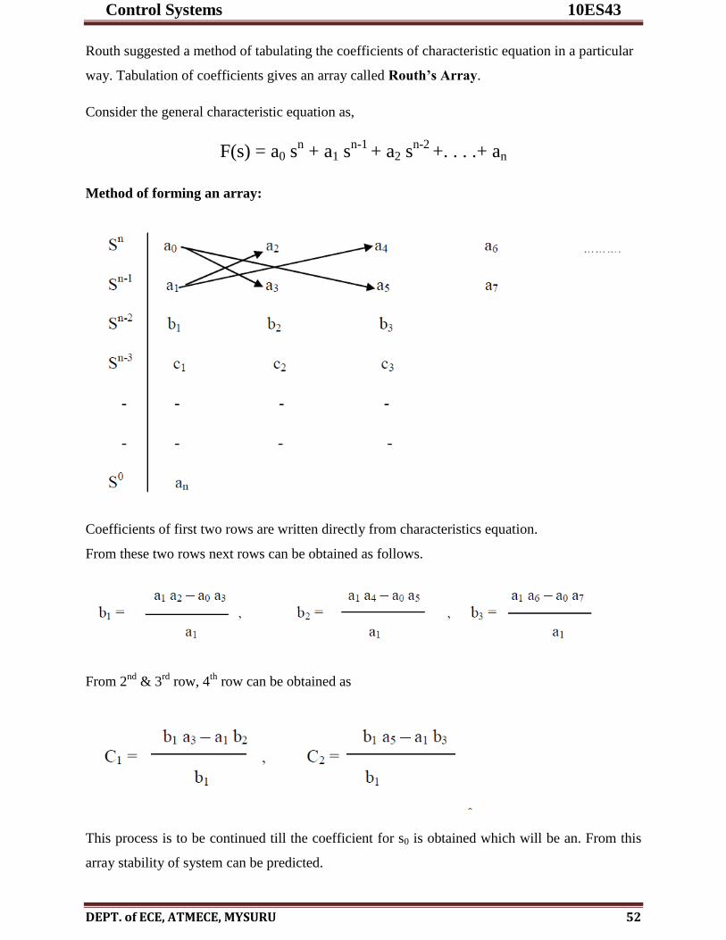
Routh suggested a method of tabulating the coefficients of characteristic equation in a particular
way. Tabulation of coefficients gives an array called Routh’s Array.
Consider the general characteristic equation as,
F(s) = a0 sn + a1 s
n-1 + a2 s
n-2 +. . . .+ an
Method of forming an array:
Coefficients of first two rows are written directly from characteristics equation.
From these two rows next rows can be obtained as follows.
From 2nd
& 3rd
row, 4th
row can be obtained as
This process is to be continued till the coefficient for s0 is obtained which will be an. From this
array stability of system can be predicted.

Control Systems 10ES43
DEPT. of ECE, ATMECE, MYSURU 53
3.5.1 Routh’s Criterion
The necessary and sufficient condition for system to be stable is “All the terms in the first
column of Routh’s array must have the same sign. There should not be any sign change in the
first column of Routh’s array.”
If there are sign changes existing then,
1. System is unstable.
2. The number of sign changes equals the number of roots lying in the right half of the s-plane.
Example 3.2: Examine stability of F(S) = S3+6S
2+11S+6=0
Solution: a0 = 1, a1 = 6, a2 =11, a3 = 6, n = 3
As there is no sign change in the first column, system is stable.
Example 3.3: Examine stability of F(S) = s3 + 4s2 + s + 16 = 0
Solution: a0 =1, a1 = 4, a2 = 1, a3 = 16
As there are two sign changes, system is unstable.
Number of roots located in the right half of s-plane = number of sign changes = 2.

Control Systems 10ES43
DEPT. of ECE, ATMECE, MYSURU 54
3.6 Special Cases of Routh’s Criterion
3.6.1 Special case 1:
First element of any of the rows of Routh’s array is zero and the same remaining row contains at
least one non-zero element.
Effect: The terms in the new row become infinite and Routh’s test fails.
Eg: s5 + 2s
4 + 3s
3 + 6s
2 + 2s + 1 = 0
Following two methods are used to remove above said difficulty.
First method: Substitute a small positive number ‘€’ in place of a zero occurred as a first
element in a row. Complete the array with this number ‘€’. Then examine the sign change by
taking Consider above Example.
To examine sign change,

Control Systems 10ES43
DEPT. of ECE, ATMECE, MYSURU 55
Routh’s array is,
As there are two sign changes, system is unstable.
Second method: To solve the above difficulty one more method can be used. In this, replace
‘S’ by ‘1/Z’ in original equation. Taking L.C.M rearrange characteristic equation in descending
powers of ‘Z’. Then complete the routh’s array with this new equation in ‘Z’ & examine the
stability with this array.
Consider F(s) = s5
+ 2s4 + 3s
3 + 6s
2 + 2s + 1 = 0
Put s = 1 / Z
Z5 + 2Z
4+ 6Z
3+3Z
2+2Z+ 1 = 0

Control Systems 10ES43
DEPT. of ECE, ATMECE, MYSURU 56
As there are two sign changes, system is unstable.
Special case 2:
All the elements of a row in Routh’s array are zero
Effect: The terms of the next row cannot be determined & Routh’s test fails
This indicates no availability of coefficient in that row.
Procedure to eliminate this difficulty:
1. Form an equation by using the coefficients of row which is just above the row of zeros.
Such an equation is called an Auxillary equation denoted as A(s). For above case such
an equation is,
A(s) = ds4 + es
2 + f
Note that the coefficients of any row are corresponding to alternate powers of ‘s’ starting from
the power indicated against it.
So ‘d’ is coefficient corresponding to s4 so first term is ds
4 of A(s).
Next coefficient ‘e’ is corresponding to alternate power of ‘s’ from 4 i.e. S2 .Hence the term es
2
& so on.
2. Taking derivative of auxillary equation with respect to ‘s’ i.e.

Control Systems 10ES43
DEPT. of ECE, ATMECE, MYSURU 57
3. Replace row of zeros by the coefficients of
4. Complete the array of zeros by the coefficients.
Importance of auxillary equation:
Auxillary equation is always the part of original characteristic equation. This means the roots of
the auxillary equation are some of the roots of original characteristics equation. Not only this but
roots of auxillary equation are the most dominant roots of the original characteristic equation,
from the stability point of view. The stability can be predicted from the roots of A(s)=0 rather
than the roots of characteristic equation as the roots of A(s) = 0 are the most dominant from the
stability point of view. The remaining roots of the characteristic equation are always in the left
half & they do not play any significant role in the stability analysis.
e.g. Let F(s) = 0 is the original characteristic equation of say order n = 5.
Let A(s) = 0 be the auxillary equation for the system due to occurrence of special case 2 of the
order m = 2.
Then out of 5 roots of F(s) = 0, the 2 roots which are most dominant (dominant means
very close to imaginary axis or on the imaginary axis or in the right half of s-plane) from the
stability point of view are the 2roots of A(s) = 0. The remaining 5 2 = 3 roots are not significant
from stability point of view as they will be far away from the imaginary axis in the left half of s-
plane.
The roots of auxillary equation may be,
1. A pair of real roots of opposite sign i.e.as shown in the fig. 3.10 (a).

Control Systems 10ES43
DEPT. of ECE, ATMECE, MYSURU 58
Fig 3.10 (a) Fig 3.10 (b)
2. A pair of roots located on the imaginary axis as shown in the fig. 3.10(b).
3. The non-repeated pairs of roots located on the imaginary axis as shown in the fig. 3.10 (c).
Fig 3.10 (C) Fig 3.10 (d)
4. The repeated pairs of roots located on the imaginary axis as shown in the Fig.3.10 (d).
Hence total stability can be determined from the roots of A(s) = 0, which can be out of
four types shown above.
Change in criterion of stability in special case 2:
After replacing a row of zeros by the coeffeicient of dA(s)/ds, Complete the Routh’s array
But now, the criterion that, no sign in 1st column of array for stability, no longer remains
sufficient but becomes a necessary. This is because though A(s) is a part of original characteristic
equation, dA(s)/ds is not, which is in fact used to complete the array.
So if sign change occurs in first column, system is unstable with number of sign changes
equal to number of roots of characteristics equation located in right half of s-plane.
But there is no sign changes, system cannot be predicted as stable. And in such case
stability is to be determined by actually solving A(s) = 0 for its roots. And from the location of
roots of A(s) = 0 in the s-plane the system stability must be determined. Because roots A(s) = 0
are always dominant roots of characteristic equation.

Control Systems 10ES43
DEPT. of ECE, ATMECE, MYSURU 59
Application of Routh’s Criterion:
Relative stability analysis :
If it is required to find relative stability of system about a line s = - i.e. how many roots are
located in right half of this line s = , the Routh’s method can be used effectively.
To determine this form Routh’s aray, shift the axis of s-plane & then apply Routh’s array
i.e substitute s=s1- (= constant) in characteristic equation. Write polynomial in terms of s1.
Complete array from this new equation. The number of sign changes in first column is equal to
number of roots those are located to right of the vertical line s = - .
Determining range of values of K:
In practical system, an amplifier of variable gain K is introduced.
The closed loop transfer function is
Hence the characteristic equation is
F(s) = 1+ KG(s) H(s) = 0
Advantages of Routh’s array are as follows:
1. Stability of the system can be judged without actually solving the characteristic equation.
2. No evaluation of determinants, which saves calculation time.
3. For unstable system it gives number of roots of characteristic equation having positive real
part.
4. Relative stability of the system can be easily judged.
Control Systems 10ES43
DEPT. of ECE, ATMECE, MYSURU 60
5. By using the criterion, critical value of system gain can be determined hence frequency of
sustained oscillations can be determined.
6. It helps in finding out range of values of K for system stability.
7. It helps in finding out intersection points of roots locus with imaginary axis.
Limitations of Routh’s criterion:
1. It is valid only for real coefficients of the characteristic equation.
2. It does not provide exact locations of the closed loop poles in left or right half of s-plane.
3. It does not suggest methods of stabilizing an unstable system.
4. Applicable only to linear system.
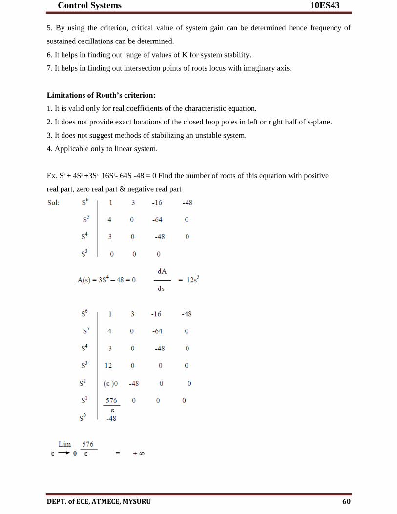
Ex. S6 + 4S5 +3S4- 16S2- 64S -48 = 0 Find the number of roots of this equation with positive
real part, zero real part & negative real part
Control Systems 10ES43
DEPT. of ECE, ATMECE, MYSURU 61
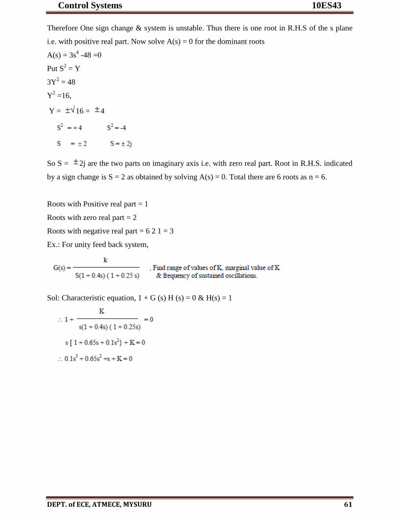
Therefore One sign change & system is unstable. Thus there is one root in R.H.S of the s plane
i.e. with positive real part. Now solve A(s) = 0 for the dominant roots
A(s) = 3s4 -48 =0
Put S2 = Y
3Y2 = 48
Y2 =16,
Y = 16 = 4
So S = 2j are the two parts on imaginary axis i.e. with zero real part. Root in R.H.S. indicated
by a sign change is S = 2 as obtained by solving A(s) = 0. Total there are 6 roots as n = 6.
Roots with Positive real part = 1
Roots with zero real part = 2
Roots with negative real part = 6 2 1 = 3
Ex.: For unity feed back system,
Sol: Characteristic equation, 1 + G (s) H (s) = 0 & H(s) = 1
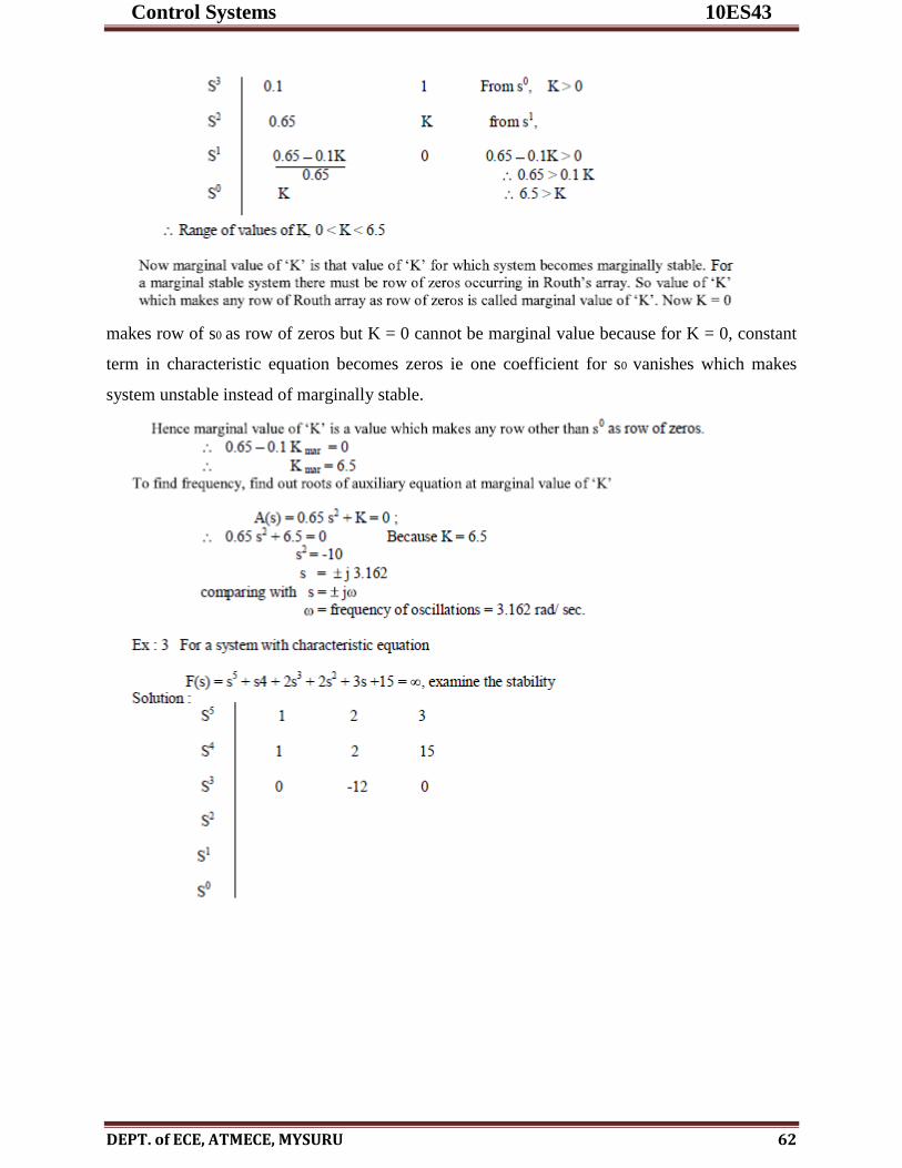
Control Systems 10ES43
DEPT. of ECE, ATMECE, MYSURU 62
makes row of s0 as row of zeros but K = 0 cannot be marginal value because for K = 0, constant
term in characteristic equation becomes zeros ie one coefficient for s0 vanishes which makes
system unstable instead of marginally stable.

Control Systems 10ES43
DEPT. of ECE, ATMECE, MYSURU 63
Ex : Using Routh Criterion, investigate the stability of a unity feedback system
whose open loop transfer function is
Sol: The characteristic equation is

Control Systems 10ES43
DEPT. of ECE, ATMECE, MYSURU 64
Now e -sT
can be Expressed in the series form as
Trancating the series & considering only first two terms we get
esT
= 1 sT
s2 + s + 1 sT = 0
s2 + s (1- T) + 1 = 0
So Routh’s array is
1-T > 0 for stability
T < 1
This is the required condition for stability of the system.
Ex : 5 Determine the location of roots with respect to s = -2 given that
F(s) = s4 + 10 s
3 + 36s
2 + 70s + 75
Sol: shift the origin with respect to s = -2
s = s1 - 2
(s - 2 ) 4 + 10 (s’- 2)
3 + 36(s’- 2 )
2 + 70 ( s’- 2) + 75 = 0

Control Systems 10ES43
DEPT. of ECE, ATMECE, MYSURU 65
Two sign change, there are two roots to the right of s = -2 & remaining ‘2’ are to the left
of the line s = -2. Hence the system is unstable.
Recommended Questions:
1. Explain briefly how system depends on poles and zeros.
2. Mention the necessary condition to have all closed loop poles in LHS of S-Plane
3. Explain briefly the hurwitz’s Criterion.
4. Explain briefly the Routh’s Stability Criterion.
5. Examine the stability of given equation using Routh’s method
s3+6s
2 + 11s + 6 =0
6. Examine the stability of given equation using Routh’s method
s5 + 2s
4 + 3s
3 + 6s
2 + 2s + 1 = 0
7. Using Routh Criterion, investigate the stability of a unity feedback system whose open loop
transfer function is

Control Systems 10ES43
DEPT. of ECE, ATMECE, MYSURU 66
3.7 Introduction to Root Locus Techniques
The characteristics of the transient response of a closed loop control system are related to
location of the closed loop poles. If the system has a variable loop gain, then the location of the
closed loop poles depends on the value of the loop gain chosen. It is important, that the designer
knows how the closed loop poles move in the s-plane as the loop gain is varied. W. R. Evans
introduced a graphical method for finding the roots of the characteristic equation known as root
locus method. The root locus is used to study the location of the poles of the closed loop transfer
function of a given linear system as a function of its parameters, usually a loop gain, given its
open loop transfer function. The roots corresponding to a particular value of the system
parameter can then be located on the locus or the value of the parameter for a desired root
location can be determined from the locus. It is a powerful technique, as an approximate root
locus sketch can be made quickly and the designer can visualize the effects of varying system
parameters on root locations or vice versa. It is applicable for single loop as well as multiple loop
system.
3.8 Root Locus Concept
To understand the concepts underlying the root locus technique, consider the second order
system shown in Fig.3.11.
Fig 3.11.Second order control system
The open loop transfer function of this system is
Where, K and a are constants. The open loop transfer function has two poles one at origin s = 0
and the other at s = -a. The closed loop transfer function of the system shown in Fig.3.11 is
The characteristic equation for the closed loop system is obtained by setting the denominator of
the right hand side of Eqn.(2) equal to zero. That is,
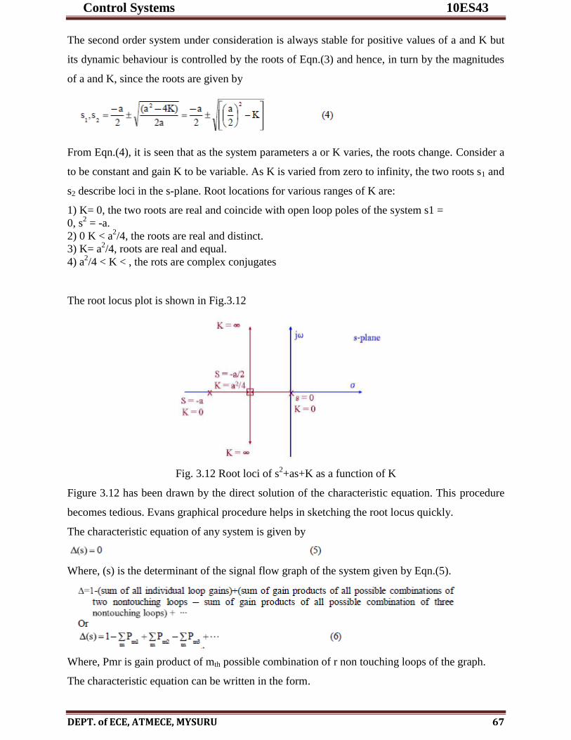
Control Systems 10ES43
DEPT. of ECE, ATMECE, MYSURU 67
The second order system under consideration is always stable for positive values of a and K but
its dynamic behaviour is controlled by the roots of Eqn.(3) and hence, in turn by the magnitudes
of a and K, since the roots are given by
From Eqn.(4), it is seen that as the system parameters a or K varies, the roots change. Consider a
to be constant and gain K to be variable. As K is varied from zero to infinity, the two roots s1 and
s2 describe loci in the s-plane. Root locations for various ranges of K are:
1) K= 0, the two roots are real and coincide with open loop poles of the system s1 =
0, s2 = -a.
2) 0 K < a2/4, the roots are real and distinct.
3) K= a2/4, roots are real and equal.
4) a2/4 < K < , the rots are complex conjugates
The root locus plot is shown in Fig.3.12
Fig. 3.12 Root loci of s2+as+K as a function of K
Figure 3.12 has been drawn by the direct solution of the characteristic equation. This procedure
becomes tedious. Evans graphical procedure helps in sketching the root locus quickly.
The characteristic equation of any system is given by
Where, (s) is the determinant of the signal flow graph of the system given by Eqn.(5).
Where, Pmr is gain product of mth possible combination of r non touching loops of the graph.
The characteristic equation can be written in the form.

Control Systems 10ES43
DEPT. of ECE, ATMECE, MYSURU 68
For single loop system shown in Fig.3.13
Where, G(s) H(s) is open loop transfer function in block diagram terminology or transmittance in
signal flow graph terminology.
Fig 3.13 Single loop feedback system
From Eqn.(7) it can be seen that the roots of the characteristic equation (closed loop poles)occur
only for those values of s where
Since, s is a complex variable, Eqn.(9) can be converted into the two Evans conditions given
below.
Roots of 1+P(s) = 0 are those values of s at which the magnitude and angle condition given by
Eqn.(10) and Eqn.(11). A plot of points in the complex plane satisfying the angle criterion is the
root locus. The value of gain corresponding to a root can be determined from the magnitude
criterion.
To make the root locus sketching certain rules have been developed which helps in visualizing
the effects of variation of system gain K ( K > 0 corresponds to the negative feedback and K < 0
corresponds to positive feedback control system) and the effects of shifting pole-zero locations
and adding in a new set of poles and zeros.
GENERAL RULES FOR CONSTRUCTING ROOT LOCUS
1) The root locus is symmetrical about real axis. The roots of the characteristic equation are
either real or complex conjugate or combination of both. Therefore their locus must be
symmetrical about the real axis.

Control Systems 10ES43
DEPT. of ECE, ATMECE, MYSURU 69
2) As K increases from zero to infinity, each branch of the root locus originates from an open
loop pole (n nos.) with K= 0 and terminates either on an open loop zero (m nos.) with K =
along the asymptotes or on infinity (zero at ). The number of branches
terminating on infinity is equal to (n- m).
3) Determine the root locus on the real axis. Root loci on the real axis are determined by open
loop poles and zeros lying on it. In constructing the root loci on the real axis choose a test point
on it. If the total number of real poles and real zeros to the right of this point is odd, then the
point lies on root locus. The complex conjugate poles and zeros of the open loop transfer
function have no effect on the location of the root loci on the real axis.
4) Determine the asymptotes of root loci. The root loci for very large values of s must be
asymptotic to straight lines whose angles are given by
5) All the asymptotes intersect on the real axis. It is denoted by a , given by
6) Find breakaway and breakin points. The breakaway and breakin points either lie on the real
axis or occur in complex conjugate pairs. On real axis, breakaway points exist between two
adjacent poles and breakin points exist between two adjacent zeros. To calculate these

Control Systems 10ES43
DEPT. of ECE, ATMECE, MYSURU 70
polynomial ds/dK =0 must be solved. The resulting roots are the breakaway / breakin points. The
characteristic equation given by Eqn.(7), can be rearranged as
The breakaway and breakin points are given by
Note that the breakaway points and breakin points must be the roots of Eqn.(15), but not all roots
of Eqn.(15) are breakaway or breakin points. If the root is not on the root locus portion of the
real axis, then this root neither corresponds to breakaway or breakin point. If the roots of
Eqn.(15) are complex conjugate pair, to ascertain that they lie on root loci, check the
corresponding K value. If K is positive, then root is a breakaway or breakin point.
7) Determine the angle of departure of the root locus from a complex pole
Angle of departure from a complex p =180o
- (sum of angles of vectors to a complex pole in question from other poles)
+ (sum of angles of vectors to a complex pole in question from other zeros) (16)
8) Determine the angle of arrival of the root locus at a complex zero
Angle of arrival at complex zero =180o
- (sum of angles of vectors to a complex Zeros in question from other Zeros)
+ (sum of angles of vectors to a complex Zeros in question from other pole) (17)
9) Find the points where the root loci may cross the imaginary axis. The points where the root
loci intersect the j axis can be found by
a) Use Routh’s Hurwitz cretion
b) letting s = in the characteristic equation , equating both the real part and imaginary part to
zero, and solving for and K. The values of thus found give the frequencies at which root loci
cross the imaginary axis. The corresponding K value is the gain at each crossing frequency.

Control Systems 10ES43
DEPT. of ECE, ATMECE, MYSURU 71
10) The value of K corresponding to any point s on a root locus can be obtained using the
magnitude condition, or
Phase Margin And Gain Margin Of Root Locus
Gain Margin
It is a factor by which the design value of the gain can be multiplied before the closed loop
system becomes unstable.
The Phase Margin
Problem No 1
Sketch the root locus of a unity negative feedback system whose forward path transfer function
Is G(s) = k/s
Solution:
1) Root locus is symmetrical about real axis.
2) There are no open loop zeros (m = 0). Open loop pole is at s = 0 (n = 1). One branch of root
locus starts from the open loop pole when K = 0 and goes to asymptotically when K .
3) Root locus lies on the entire negative real axis as there is one pole towards right of any point
on the negative real axis.
4) The asymptote angle is

Control Systems 10ES43
DEPT. of ECE, ATMECE, MYSURU 72
Angle of asymptote is
5) Centroid of the asymptote is
6) The root locus does not branch. Hence, there is no need to calculate the break points.
7) The root locus departs at an angle of -180 from the open loop pole at s = 0.
8) The root locus does not cross the imaginary axis. Hence there is no imaginary axis cross over.
The root locus plot is shown in Fig.3.14
Fig 3.14: Root locus plot of K/s
Comments on stability:
The system is stable for all the values of K > 0. Th system is over damped.

Control Systems 10ES43
DEPT. of ECE, ATMECE, MYSURU 73
Problem No 2
The open loop transfer function is given below. Sketch the root locus plot
Solution:
1) Root locus is symmetrical about real axis.
2) There is one open loop zero at s=-2.0(m=1). There are two open loop poles at
s=-1, -1(n=2). Two branches of root loci start from the open loop pole when
K= 0. One branch goes to open loop zero at s =-2.0 when K -> and other goes to (open loop
zero ) asymptotically when K .
3) Root locus lies on negative real axis for s -2.0 as the number of open loop poles plus
number of open loop zeros to the right of s=-0.2 are odd in number.
4) The asymptote angle is
Angle of asymptote is
5) Centroid of the asymptote is
6) The root locus has break points.

Control Systems 10ES43
DEPT. of ECE, ATMECE, MYSURU 74
The root loci brakesout at the open loop poles at s=-1, when K =0 and breaks in onto the real axis
at s=-3, when K=4. One branch goes to open loop zero at s=-2 and other goes to along the
asymptotically.
7) The branches of the root locus at s=-1, -1 break at K=0 and are tangential to a line s= - 1+j0
hence depart at 90.
8) The locus arrives at open loop zero at 180.
9) The root locus does not cross the imaginary axis, hence there is no need to find the imaginary
axis cross over. The root locus plot is shown in Fig.3.15.
Fig 3.15: Root locus plot for K(S+2)/(S+1)2
Comments on stability:
System is stable for all values of K > 0. The system is over damped for K > 4. It is critically
damped at K = 0, 4.
Problem No 3
The open loop transfer function is given below. Sketch the root locus.
Solution:
1) Root locus is symmetrical about real axis.

Control Systems 10ES43
DEPT. of ECE, ATMECE, MYSURU 75
2) There are one open loop zero at s=-4(m=1). There are two open loop poles at s=0, -2(n=2).
Two branches of root loci start from the open loop poles when K= 0. One branch goes to open
loop zero when K and other goes to infinity asymptotically when
and other goes to infinity asymptotically when
3) Entire negative real axis except the segment between s=-4 to s=-2 lies on the root locus.
4) The asymptote angle is
Angle of asymptote are
5) Centroid of the asymptote is
6) The brake points are given by dK/ds =0.
7) Angle of departure from open loop pole at s =0 is 180o. Angle of departure from pole at s=-2.0
is 0 .
8) The angle of arrival at open loop zero at s=-4 is 180o.
9) The root locus does not cross the imaginary axis. Hence there is no imaginary cross over.
The root locus plot is shown in fig.3.16

Control Systems 10ES43
DEPT. of ECE, ATMECE, MYSURU 76
Fig 3.16: Root locus plot of K(s+4)/s(s+2)
Comments on stability:
System is stable for all values of K.
Problem No 4
The open loop transfer function is given below. Sketch the root locus.
Solution:
1) Root locus is symmetrical about real axis.
2) There is one open loop zero at s = -0.2(m=1). There are three open loop poles at
s = 0, 0, -3.6(n=3). Three branches of root loci start from the three open loop poles when K= 0
and one branch goes to open loop zero at s = -0.2 when and other two go to
asymptotically when .
3) Root locus lies on negative real axis between -3.6 to -0.2 as the number of open loop poles plus open zeros to the right of any point on the real axis in this range is odd.

Control Systems 10ES43
DEPT. of ECE, ATMECE, MYSURU 77
4) The asymptote angle is
Angle of asymptote are
5) Centroid of the asymptote is
6) The root locus does branch out, which are given by dK/ds =0.
The root loci brakeout at the open loop poles at s = 0, when K =0 and breakin onto the real axis
at s=-0.432, when K=2.55 One branch goes to open loop zero at s=-0.2 and other goes breaksout
with the another locus starting from open loop ploe at s= -3.6. The break point is at s=-1.67 with
K=3.66. The loci go to infinity in the complex plane with constant real part s= -1.67.
7) The branches of the root locus at s=0, 0 break at K=0 and are tangential to imaginary axis or
depart at 90. The locus departs from open loop pole at s=-3.6 at 0.
8) The locus arrives at open loop zero at s=-0.2 at 180 .
9) The root locus does not cross the imaginary axis, hence there is no imaginary axis cross over.
The root locus plot is shown in Fig.3.17.
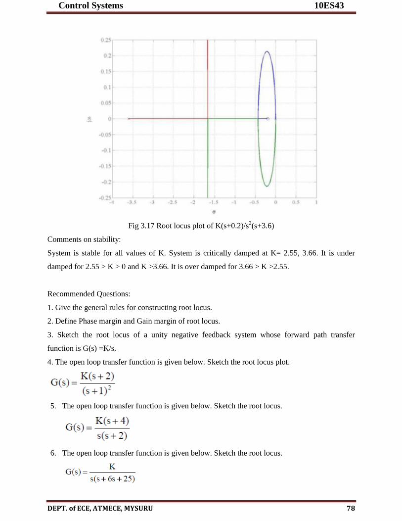
Control Systems 10ES43
DEPT. of ECE, ATMECE, MYSURU 78
Fig 3.17 Root locus plot of K(s+0.2)/s2(s+3.6)
Comments on stability:
System is stable for all values of K. System is critically damped at K= 2.55, 3.66. It is under
damped for 2.55 > K > 0 and K >3.66. It is over damped for 3.66 > K >2.55.
Recommended Questions:
1. Give the general rules for constructing root locus.
2. Define Phase margin and Gain margin of root locus.
3. Sketch the root locus of a unity negative feedback system whose forward path transfer
function is G(s) =K/s.
4. The open loop transfer function is given below. Sketch the root locus plot.
5. The open loop transfer function is given below. Sketch the root locus.
6. The open loop transfer function is given below. Sketch the root locus.
Control Systems 10ES43
DEPT. of ECE, ATMECE, MYSURU 79
7. The open loop transfer function is given below. Sketch the root Locus

Control Systems 10ES43
DEPT. of ECE, ATMECE, MYSURU 80
MODULE 4
FREQUENCY DOMAIN ANALYSIS AND STABILITY
4.1 Bode plots
Bode plots are graphs of the steady state response of stable continuous time Linear time
invariant systems for sinusoidal inputs, plotted as change in magnitude and phase versus
frequency on logarithmic scale. Bode plots are a visual description of the system. So, these
Bode plots are used for the representation of sinusoidal transfer function . In this
representation the magnitude of G(jω) in db, i.e, 20 log G(jω) is plotted against 'log ω'.
Similarly phase angle of G(jω) is plotted against 'log ω' .Hence the abscissa is logarithm of the
frequency and hence the plots are known as logarithmic plots. The plots are named after the
famous mathematician H. W. Bode.
The transfer function G(jω) can be written as G(jω) = G(jω)∟Ф( ω) Where Ф( ω) is the angle
G(jω) .
Since G(jω) consists of many multiplicative factors in the numerator and denominator it is
convenient to take logarithm of G(jω) to convert these factors into additions and subtractions,
which can be carried out easily.
4.1.1 Magnitude Plot
To plot the magnitude plot , magnitude is plotted against input frequency on a logarithmic
scale.It can be approximated by two lines and it forms the asymptotic (approximate) magnitude
Bode plot of the transfer function:
(i) for angular frequencies below ωc it is a horizontal line at 0 dB since at low frequencies the
term ω / ωc is small and can be neglected, making the decibel gain equation above equal to
zero,

Control Systems 10ES43
DEPT. of ECE, ATMECE, MYSURU 81
(ii) for angular frequencies above ωc it is a line with a slope of −20 dB per decade since at
high frequencies the term ω / ωc dominates and the decibel gain expression above simplifies to
-20 log (ω / ωc ) which is a straight line with a slope of −20 dB per decade.
These two lines meet at the corner frequency. From the Bode plot, it can be seen that for
frequencies well below the corner frequency, the circuit has an attenuation of 0 dB,
corresponding to a unity pass band gain, i.e. the amplitude of the filter output equals the
amplitude of the input. Frequencies above the corner frequency are attenuated – the higher the
frequency, the higher the attenuation.
4.1.2 Phase plot
The phase Bode plot is obtained by plotting the phase angle of the transfer function given by
Φ = - tan –
(ω/ωc ) Versus ω ,
Where, ω and ωc are the input and cutoff angular frequencies respectively.
For input frequencies much lower than corner, the ratio ω/ωc is small and therefore the phase
angle is close to zero. As the ratio increases the absolute value of the phase increases and
becomes –45 degrees when ω= ωc . As the ratio increases for input frequencies much greater
than the corner frequency, the phase angle asymptotically approaches −90 degrees. The
frequency scale for the phase plot is logarithmic.
The main advantage of using the Bode plots is that multiplication of magnitudes can be
converted into addition. Also a simple method of plotting an approximate log-magnitude curve is
obtained. It is based on asymptotic approximations. Such approximation by straight line
asymptotes is sufficient if only rough information on the frequency response characteristics is
needed. The phase angle curves can be drawn easily if a template for the phase angle curve of
1+jω is available. Expanding the low frequency range ,by use of a logarithmic scale for the
frequency is very advantageous ,since characteristics at low frequencies are most important in
practical systems. The only limitation is ,it is not possible to draw the curve ,right down to zero
frequency because of the logarithmic frequency (log 0 = ∞) .But this do not give any serious
problem.
4.2 Polar plot
This plot is drawn to study the frequency response in polar co-ordinates. The polar plot of a
sinusoidal transfer function G(jω) is a plot of the magnitude of G(jω) Vs the phase of G(jω) on
polar co-ordinates as ω is varied from 0 to ∞. Polar graph sheet has concentric circles and radial
lines. Concentric circles represent the magnitude. Radial lines represents the phase angles. In

Control Systems 10ES43
DEPT. of ECE, ATMECE, MYSURU 82
polar sheet +ve phase angle is measured in ACW from 00
and -ve phase angle is measured in
CW from 00
.
To sketch the polar plot of G(jω) for the entire range of frequency ω, i.e., from 0 to infinity, there
are four key points that usually need to be known:
The start of plot where ω = 0,
The end of plot where ω = ∞,
where the plot crosses the real axis, i.e., Im(G(jω)) = 0, and
where the plot crosses the imaginary axis, i.e., Re(G(jω)) = 0.
Procedure: The following steps are involved in the plotting of Polar graphs
Express the given expression of OLTF in (1+sT) form.
Get the expressions for | G(jω)H(jω)| & G(jω)H(jω).
Tabulate various values of magnitude and phase angles for different values of ω ranging
from 0 to ∞.
Usually the choice of frequencies will be the corner frequency and around corner
frequencies. Choose proper scale for the magnitude circles.
Fix all the points in the polar graph sheet and join the points by a smooth curve.
Write the frequency corresponding to each of the point of the plot.
4.2.1 Gain Margin
Gain Margin is defined as “the factor by which the system gain can be increased to drive the
system to the verge of instability”.
For stable systems, ωgc < ωpc
│G(j)H(j)│ at ω= ωpc < 1
GM = in positive dB .
More positive the Gain Margin , more stable is the system
For marginally stable systems, ωgc = ωpc │G(j)H(j)│ at ω=ωpc = 1
GM = 0 dB
For Unstable systems, ωgc > ωpc
│G(j)H(j)│ at ω=ωpc > 1
GM = in negative dB
Control Systems 10ES43
DEPT. of ECE, ATMECE, MYSURU 83
Gain is to be reduced to make the system stable
The important conclusions are :
If the gain is high, the GM is low and the system’s step response shows high overshoots
and long settling time.
On the contrary, very low gains give high GM and PM, but also causes higher ess(Error),
higher values of rise time and settling time and in general give sluggish response.
Thus we should keep the gain as high as possible to reduce ess and obtain acceptable
response speed and yet maintain adequate GM and PM.
As a thumb rule an adequate GM of 2 ( ie 6 dB ) and a PM of about 30 is generally
considered sufficient enough.
If the gain of the system is increased by a factor 1/β, then the G(j)H(j) at ω=ωpc becomes
β(1/β) = 1 and hence the │G(j)H(j)│ locus pass through -1+j0 point driving the system to
the verge of instability
4.2.2 PHASE MARGIN
Phase Margin is defined as “the additional phase lag that can be introduced before the system
becomes unstable”.
Let ‘A’ be the point of intersection of │G(j)H(j)│ plot and a unit circle centered at the
origin.
Draw a line connecting the points ‘O’ & ‘A’ and measure the phase angle between the
line OA and +ve real axis. This angle is the phase angle of the system at the gain cross
over frequency.ے G(jωgc)H(jgc) = Фgc
If an additional phase lag of PM is introduced at this frequency, then the phase angle
G(jωgc)H(jωgc) will become 180 and the point ‘A‘ coincides with (-1+j0) driving the
system to the verge of instability.
This additional phase lag is known as the Phase Margin.

Control Systems 10ES43
DEPT. of ECE, ATMECE, MYSURU 84
For a stable system, the phase margin is positive.
A Phase margin close to zero corresponds to highly oscillatory system
A polar plot may be constructed from experimental data or from a system transfer
function
If values of ω are marked along the contour, a polar plot gives the same information as a
Bode plot
Usually, the shape of a polar plot is very important as it gives much information about the
system.
4.3 Relative and absolute stability A stable system is a dynamic system with a bounded response to a bounded input. A necessary
and sufficient condition for a feedback system to be stable is that all the poles of the system
transfer function have negative real parts
A system is considered marginally stable if only certain bounded inputs will result in a bounded
output. In practical systems, it is not sufficient to know that the system is stable but a stable
system must meet the specifications of relative stability which is a quantitative measure of how
fast the transients die out in the system.
Relative stability of a system is usually defined in terms of two design parameters-phase margin
and gain margin.The relative stability of a system can be defined as the property that is measured
by the relative real part of each root or pair of roots. The relative stability of a system can also be
defined in terms of the relative damping coefficients of each complex root pair and, therefore, in
terms of the speed of response and overshoot instead of settling time.

Control Systems 10ES43
DEPT. of ECE, ATMECE, MYSURU 85
4.4 Time Domain Analysis Vs Frequency Domain Analysis
Variable frequency, sinusoidal signal generators are readily available and precision
measuring instruments are available for measurement of magnitude and phase angle. The
time response for a step input is more difficult to measure with accuracy.
It is easier to obtain the transfer function of a system by a simple frequency domain
test.Obtaining transfer function from the step response is more tedious.
If the system has large time constants, it makes more time to reach steady state at each
frequency of the sinusoidal input. Hence time domain method is preferred over frequency
domain method in such systems.
In order to do a frequency response test on a system, the system has to be isolated and the
sinusoidal signal has to be applied to the system. This may not be possible in systems
which can not be interrupted. In such cases, a step signal or an impulse signal may be
given to the system to find its transfer function. Hence for systems which cannot be
interrupted, time domain method is more suitable.
The design of a controller is easily done in the frequency domain method than in time
domain method. For a given set of performance measures in frequency domain , the
parameters of the open loop transfer function can be adjusted easily.
The effect of noise signals can be assessed easily in frequency domain rather than time
domain.
The most important advantage of frequency domain analysis is the ability to obtain the
relative stability of feedback control systems. The Routh Hurwitz criterion is essentially
a time do main method which determines the absolute stability of a system.
Since the time response and frequency response of a system are related through Fourier
transform , the time response can be easily obtained from the frequency response. The
correlation between time and frequency response can be easily established so that the
time domain performance measures can be obtained from the frequency domain
specifications and vice versa.

Control Systems 10ES43
DEPT. of ECE, ATMECE, MYSURU 86
4.4 Frequency Response of a Control System :
To study the frequency response of a control system let us consider second order system with the
transfer function,
The steady state sinusoidal response is obtained by substituting s = j ω in the above equation
Normalizing the frequency ω, with respect to the natural frequency ωn by defining a variable
We have,
From the above equation the magnitude and angle of the frequency response is obtained as,
and
The time response for a unit sinusoidal input with frequency OJ is given by,
The magnitude and phase of steadystate sinusoidal response for variable frequency can be
plotted and are shown in the Fig. (a) and (b).
Control Systems 10ES43
DEPT. of ECE, ATMECE, MYSURU 87
An important performance measure, in frequency domain, is the bandwidth of the system.
From Fig. , we observe that for δ < 0.707 and U > Ur the magnitude decreases monotonically.
The frequency Ub where the magnitude becomes 0.707 is known as the cut off frequency. At
this frequency, the magnitude will be

Control Systems 10ES43
DEPT. of ECE, ATMECE, MYSURU 88
4.5 Nyquist Criteria
A stability test for time invariant linear systems can also be derived in the frequency domain. It is
known as Nyquist stability criterion. It is based on the complex analysis result known as
Cauchy’s principle of argument.
The Nyquist stability criterion relates the location of the roots of the characteristic equation to
the open-loop frequency response of the system. In this, the computation of closed-loop poles is
not necessary to determine the stability of the system and the stability study can be carried out
graphically from the open-loop frequency response. Therefore experimentally determined open-
loop frequency response can be used directly for the study of stability. When the feedback path is
closed. The Nyquist criterion provides the information on absolute and relative stability of the
system.

Control Systems 10ES43
DEPT. of ECE, ATMECE, MYSURU 89
Let us suppose that the system transfer function is a complex function. By applying Cauchy’s
principle of argument to the open-loop system transfer function, we will get information about
stability of the closed-loop system transfer function and arrive at the Nyquist stability criterion
The importance of Nyquist stability lies in the fact that it can also be used to determine the
relative degree of system stability by producing the so-called phase and gain stability margins.
These stability margins are needed for frequency domain controller design techniques
The Nyquist plot is a polar plot of the function D(s) = 1 = G(s).H(s)
The Nyquist criterion states that the number of unstable closed-loop poles is equal to the
number of unstable open-loop poles plus the number of encirclements of the origin of the
Nyquist plot of the complex function D(s).
4.6 Control system Compensators
A control system is usually required to meet three time response specifications, namely, steady
state accuracy, damping factor and settling time. To get the desired design with minimum errors
and to adjust the parameters of the overall system to satisfy the design criterion an additional
subsystem called 'Compensator ‘ must be used.
This compensator may be used in series with the plant in the forward path or in the feedback
path shown in Fig. below. The compensation in the forward path is known as series or cascade
compensation and the later is known as feedback compensation. The compensator may be a
passive network or an active network.
Series compensation Feedback compensation
In general the series compensation is much simpler than the feed back compensation.But the
series compensation frequently require additional amplifiers to increase the gain and to provide
isolation.i.e to avoid power dissipation the series compensator is inserted in the lowest energy
point in the feed forward path.In general the number of components required in feed back
compensation will be less than the number of components in series compensation.
Control Systems 10ES43
DEPT. of ECE, ATMECE, MYSURU 90
There are three important types of compensators.(i) Lead Compensator (ii) Lag compensator and
(iii) Lag-Lead compensator.
In a network ,when a sinusoidal input signal ei is applied at its input and if the steady state
output eo has a phase lead then the network is called a lead network. Similarly In the network for
a sinusoidal input ei ,if the steady state output has a phase lag ,then the network is called a lag
network.
Similarly in a network for a sinusoidal input .if the steady state out put has both phase lag and
lead ,but different frequency regions ,then the network is called lag-lead network. Generally the
phase lag occurs at low frequency regions and the phase lead occurs at higher frequency region.
A compensator having the characteristics of a lead network , lag network or lead-lag network is
called a lead compensator ,lag compensator or lag-lead compensator.
The lead compensators, lag compensators and lag-lead compensators are be designed either
using electronic components like operational amplifiers or using Root Locus methods. The first
type are called electronic lag compensators .The second type are Root locus compensators. The
Root locus compensators are have many advantages over electronic type.
Lead compensation basically speeds up the response of the control system and increase the
stability of the system. Lag compensation improves the steady –state accuracy of the system but
reduces the speed of the response. If improvements in both transient response and steady state
response is required ,both lead compensator and lag compensator are used simultaneously .In
general using a single lag-lead compensator is always economical.
Lag-lead compensation combines the advantage of lag and lead compensation. Since, the lag –
lead compensator possesses two poles and two zeros ,such a compensation increases the order of
the system by 2 ,unless the cancellation of the poles and zeros occurs in the compensated system.
4.6.1 Lead Compensator
It has a zero and a pole with zero closer to the origin. The general form of the transfer function of
the load compensator is,

Control Systems 10ES43
DEPT. of ECE, ATMECE, MYSURU 91
Subsisting

Control Systems 10ES43
DEPT. of ECE, ATMECE, MYSURU 92
Transfer function s
4.6.2 Lag Compensator
It has a zero and a pole with the zero situated on the left of the pole on the negative real axis. The
general form of the transfer function of the lag compensator is
Therefore, the frequency response of the above transfer function will be
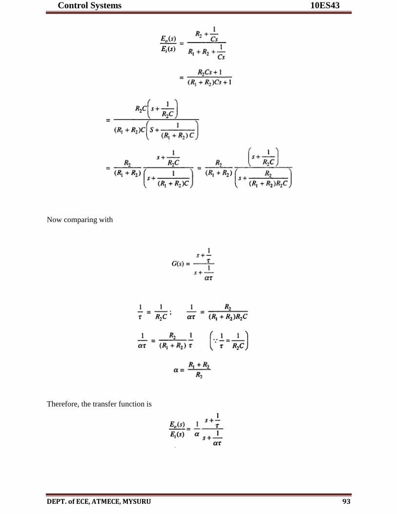
Control Systems 10ES43
DEPT. of ECE, ATMECE, MYSURU 93
Now comparing with
Therefore, the transfer function is

Control Systems 10ES43
DEPT. of ECE, ATMECE, MYSURU 94
4.6.3 Lag-Lead Compensator
The lag-lead compensator is the combination of a lag compensator and a lead compensator. The
lag-section is provided with one real pole and one real zero, the pole being to the right of zero,
whereas the lead section has one real pole and one real zero with the zero being to the right of
the pole.
The transfer function of the lag-lead compensator will be
The figure below shows the lag lead compensator
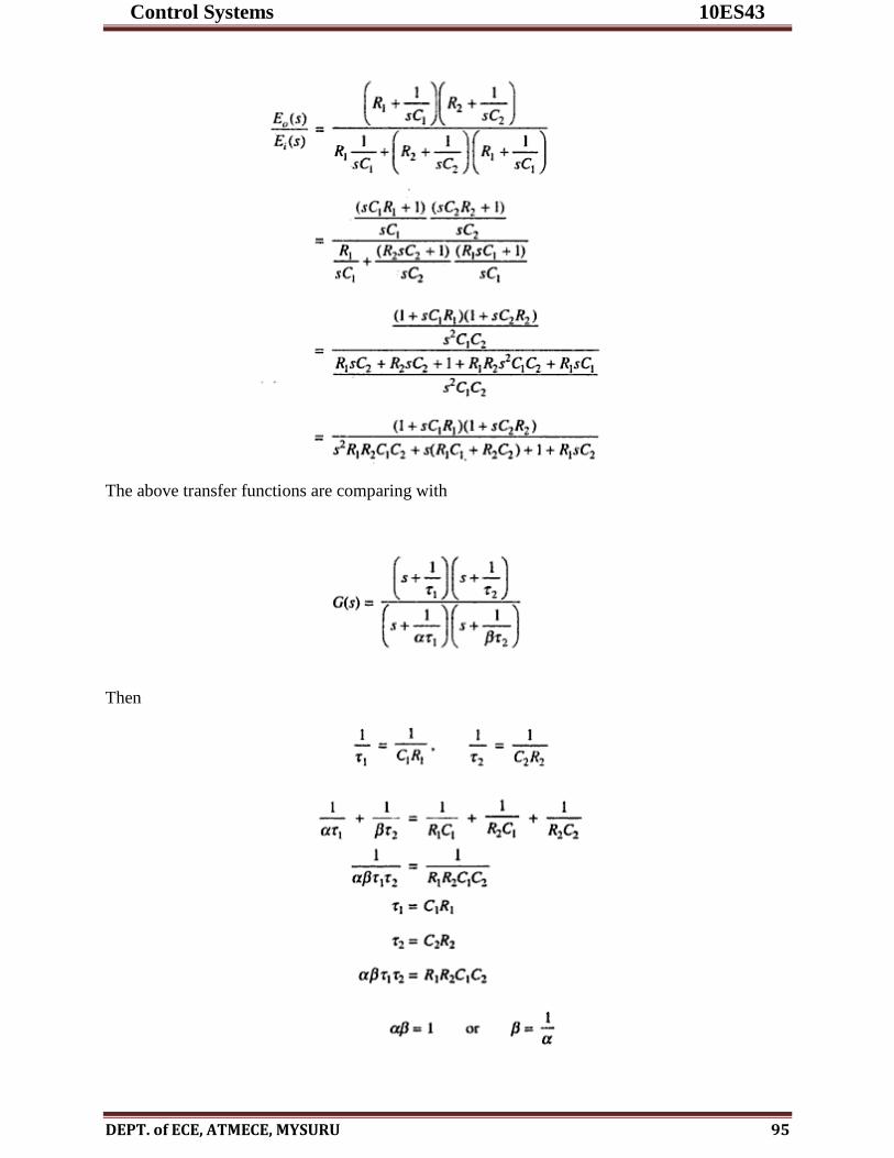
Control Systems 10ES43
DEPT. of ECE, ATMECE, MYSURU 95
The above transfer functions are comparing with
Then

Control Systems 10ES43
DEPT. of ECE, ATMECE, MYSURU 96
Therefore, the transfer function is given by

Control Systems 10ES43
DEPT. of ECE, ATMECE, MYSURU 97
MODULE 5
STATE VARIABLE ANALYSIS
Analysis and the design of feedback control systems by the classical design methods (root locus
and frequency domain methods) based on the transfer function approach are inadequate and not
convenient. So, the development of the state-variable approach, took place .This methos has
the following advantages over the classical approach.
1. It is a direct time-domain approach. Thus, this approach is suitable for digital computer
computations
2. It is a very powerful technique for the design and analysis of linear or nonlinear, time-variant
or time-invariant, and SISO or MIMO systems.
3. In this technique, the nth
order differential equations can be expressed as ‘n’ equations of first
order. Thus, making the solutions easier.
4. Using this approach, the system can be designed for optimal conditions with respect to given
performance indices.
5.1 Definitions:
State : The state of a dynamical system is a minimal set of variables x1(t), x2(t)x3(t) …xn(t)
such that the knowledge of these variables at t = t0 (initial condition), together with the
Knowledge of inputs u1(t), u2(t), u3(t)… um (t) for t ≥0, completely determines the behavior of
the system for t < t0.
State-Variables :
The variables x1(t),x2(t),x3(t)… xm(t) such that the knowledge of these variables at t = t0 (initial
condition), together with the knowledge of inputs u1(t), u2(t), u3(t)… um(t) for t ≥ t0, completely
determines the behavior of the system for t < t0 ; are called state-variables. In other words, the
variables that determine the state of a dynamical system, are called state-variables.
State-Vector :
If n state variables x1(t), x2(t), x3(t)… xn(t) are necessary to determine the behavior of a
dynamical system, then these n state-variables can be considered as n components of a vector
x(t), called state-vector.
State-Space : The n dimensional space, whose elements are the n state-variables, is called state-
space. Any state can be represented by a point in the state-space.

Control Systems 10ES43
DEPT. of ECE, ATMECE, MYSURU 98
5.2 State equation of a linear time-invariant system
For a general system of the Figure shown below the state representation can be arranged in the
form of n first-order differential equations as
……(5.1)
Integrating equation 5.1 , we get
Where I = 1,2,3……..n
Thus, the n state-variables and, the state of the system can uniquely be determined at any t < tn,
provided each state-variable is known at t = tn and all the m control forces are known throughout
the interval t 0 to t.
The n differential equations of 1 may be written in vector form as
………… (5.2)

Control Systems 10ES43
DEPT. of ECE, ATMECE, MYSURU 99
Equation 5. 2 is the state equation for time-invariant systems. However, for time-varying
systems, the function vector f(.) is dependent on time as well, and the vector equation may be
given as ……………….(5.3)
Equation (5.3) is the state equation for time-varying systems.
The output y(t) can, in general, be expressed in terms of the state vector x(t) and input vector u(t)
as ,
For time-invariant systems :
------------------------ -----(5.4)
For time-varying systems: ----------------(5.5)
5.3 STATE MODEL OF A LINEAR SINGLE-INPUT-SINGLE-OUTPUT
SYSTEM
The state model of a linear single-input-single-output system can be written as
(5.6)
(5.7)
Where

Control Systems 10ES43
DEPT. of ECE, ATMECE, MYSURU 100
d = Transmission Constant , u(t) = Input or Control Variable (scalar)
and, y(t) = Output Variable (scalar).
A very important conclusion is that the derivatives of all the state-variables are zero at the
equilibrium point. Thus, the system continues to lie at the equilibrium point unless otherwise
disturbed.
5.6 SOLUTION OF STATE EQUATIONS FOR LINEAR TIME-
INVARIANT SYSTEMS
The state equation of a linear time-invariant system is given by
For a homogeneous (unforced) system
So , we have ………..(5.8)
Take the Laplace Transform on both sides
…………… (5.9)
The above may also be written as
Taking the inverse Laplace transform --------------(5.10)

Control Systems 10ES43
DEPT. of ECE, ATMECE, MYSURU 101
This equation (3) gives the solution of the LTI homogeneous state Equation. It can be observed
that the initial state x(0) at t = 0, is driven to a state x(t) at time t. This transition in state is carried
out by the matrix exponential eAt. Because of this property, eA
t is termed as the State Transition
Matrix and is denoted by ø(t).
5.7 Determination of transfer function using SVA
Let us consider the following state space equation ,
Now, take the Laplace Transform (with zero initial conditions)
We want to solve for the ratio of Y(s) to U(s), which gives the transfer function.So, we need to
remove Q(s) from the output equation. We solve the state equation for Q(s)
The matrix Φ(s) is called the state transition matrix. Now , put this into the output equation
Now solving for transfer function ,we get
This is the method of determining the transfer function from state variable analysis (SVA).


![Ece IV Control Systems [10es43] Notes1](https://img.dokumen.tips/doc/110x75/55cf98ff550346d0339aef46/ece-iv-control-systems-10es43-notes1.jpg)


![Eee IV Control Systems [10es43] Notes](https://img.dokumen.tips/doc/110x75/55cf9c1d550346d033a8a65c/eee-iv-control-systems-10es43-notes.jpg)


![Ece-IV-control Systems [10es43]-Question Paper](https://img.dokumen.tips/doc/110x75/55cf96ef550346d0338ebf13/ece-iv-control-systems-10es43-question-paper.jpg)


![Ece IV Control Systems [10es43] Notes](https://img.dokumen.tips/doc/110x75/55cf96ef550346d0338ebd82/ece-iv-control-systems-10es43-notes.jpg)
