INTERNATIONAL JOURNAL OF PROFESSIONAL ENGINEERING STUDIES Volume VI /Issue 3 / MAY 2016

IJPRES

CONTROL STRATEGY FOR RENEWABLE POWER INTEGRATION TO THE DC MICRO GRID

M.BALAJYOTHI*, N.PHANI KUMAR**

M.Bala Jyothi,M.Tech(PE),Department of Electrical and Electronics Engineering, Eluru College of Engineering and Technology,Eluru,West Godavari(Dt), A.P., India

E-mail: balajyothi33@gmail.com N.Phani Kumar,Assistant Professor, Department of Electrical and Electronics Engineering,

Eluru College of Engineering and Technology,Eluru,West Godavari(Dt), A.P., India E-mail: npk235@gmail.com

ABSTRACT- Several operational controls are designed to support the integration of renewable energy sources within microgrids. An aggregated model of renewable wind and solar power generation forecast is proposed to support the quantification of the operational reserve for day-ahead and real-time scheduling. The power which can be produced from the renewable sources will be synchronized to the ac grid or directly to dc consumers. In these operation BESS (battery energy storage system)is equipped with the system for maintaining the power balance. For obtaining the power balance the adaptive droop control technique has to be proposed and droop curves are evaluated. The droop characteristics are selected on the basis of the deviation between the optimized and real-time SOC of the BESS. Then, a droop control for power electronic converters connected to battery storage is developed using fuzzy logic controller and tested. Compared with the existing droop controls, it is distinguished in that the droop curves are set as a function of the storage state-of-charge (SOC) and can become asymmetric. The controls are implemented for the special case of a dc microgrid that is vertically integrated within a high-rise host building of an urban area. Index Terms—Distributed energy resources, droop control, electric vehicle (EV), microgrid, multilevel energy storage, fuzzy logic controller, power electronic conversion, solar power, wind power.

I. INTRODUCTION Wind is abundant almost in any part of the world. Its existence in nature caused by uneven heating on the surface of the earth as well as the earth’s rotation means that the wind resources will always be available. The trend has been toward increasingly larger turbine sizes, culminating in the installation of off-shore wind parks that are located far from the load centers [2]. This can lead to rather large distances between generation and load in the electricity sector. The transportation sector reveals an even larger disconnect between the locations of fuel

production and consumption. The energy system proposed in this paper seeks to address both issues related to electricity and transportation sectors. One potential solution is a microgrid that can be vertically integrated with a high-rise building as frequently encountered in urban areas. The harvesting of renewable wind and solar energy occurs at the top of the building. The rooftop generation connects to the ground level via a microgrid where electric vehicle (EV) charging stations are supplied, and a battery supports maintaining the balance of supply and demand. The potential value of an urban integration within buildings as considered here comes from the usage of rooftop energy resources, the storage of the latter for offering EV fast charging at the ground level, the contribution to emission-free EV transportation in urban areas, the co-location and integration of generation and load in urban areas, and the grid-friendly integration of the microgrid with the rest of the power system main grid. The combination of wind and solar energy resources on a rooftop was also investigated in [3]. It was verified that the combination of wind and solar energy leads to reduced local storage requirements [4]. The combination of diverse but complementary storage technologies in turn can form a multilevel energy storage, where a supercapacitor or flywheel provides cache control to compensate for fast power fluctuations and to smoothen the transients encountered by a battery with higher energy capacity [5], [6]. Microgrids or hybrid energy systems have been shown to be an effective structure for local interconnection of distributed renewable generation, loads, and storage [7]–[12]. Recent research has considered the optimization of the operation on one hand [13]–[15] and the usage of dc to link the resources on the other [16]–[18]. The dc link voltage was shown to be maintained by a droop control that relates the dc link voltage to the power output of controllable resources. In this paper, it is proposed to set the droop as a function of

INTERNATIONAL JOURNAL OF PROFESSIONAL ENGINEERING STUDIES Volume VI /Issue 3 / MAY 2016

IJPRES

the expected state of charge (SOC) of the battery according to its operational optimization set point versus the actual realtime SOC. The proposed operational optimization is further distinguished in that it quantifies the uncertainty associated with renewable generation forecast, emission constraints, and EV fast charging.

Fig. 1. Layout of the dc microgrid Following this introduction, an outline of the principle of a dc microgrid is given in Section II. In Section III, a method is developed for quantifying the aggregated wind and solar power forecast uncertainty, the resulting required SOC of the battery, and the operational optimization. The optimization guided droop control is dealt with in Section IV. A case study involving a time series and simulation over diverse time scales to substantiate the claims made is discussed in Section V. Conclusions are drawn in Section VI.

II. OUTLINE OF DC MICROGRID A schematic of the dc microgrid with the conventions employed for power is given in Fig. 1. The dc bus connects wind energy conversion system (WECS), PV panels, multilevel energy storage comprising battery energy storage system (BESS) and supercapacitor, EV smart charging points, EV fast charging station, and grid interface. The WECS is connected to the dc bus via an ac–dc converter. PV panels are connected to the dc bus via a dc–dc converter. The BESS can be realized through flow battery technology connected to the dc bus via a dc–dc converter. The supercapacitor has much less energy capacity than the BESS. Rather, it is aimed at compensating for fast fluctuations of power and so provides cache control as detailed in [19]. Thanks to the multilevel energy storage, the intermittent and volatile renewable power outputs can be managed, and a deterministic controlled power to the main grid is obtained by optimization. Providing uninterruptible power supply (UPS) service to loads

when needed is a core duty of the urban microgrid. EV fast charging introduces a stochastic load to the microgrid. The multilevel energy storage mitigates potential impacts on the main grid. In building integration, a vertical axis wind turbine may be installed on the rooftop as shown in Fig. 2. PV panels can be co-located on the rooftop and the

Fig. 3. Overview of optimized scheduling approach facade of the building. Such or similar configurations benefit from a local availability of abundant wind and solar energy. The fast charging station is realized for public access at the ground level. It is connected close to the LV–MV transformer to reduce losses and voltage drop. EVs parked in the building are offered smart charging within user-defined constraints. III. OPERATIONAL OPTIMIZATION OF MICROGRID FOR RENEWABLE ENERGY INTEGRATION

The algorithm for optimized scheduling of the microgrid is depicted in Fig. 3. In the first stage, wind and solar power generation are forecast. The uncertainty of the wind and solar power is presented by a three-state model. An example of such a forecast

INTERNATIONAL JOURNAL OF PROFESSIONAL ENGINEERING STUDIES Volume VI /Issue 3 / MAY 2016

IJPRES

Fig.4. Wind or solar power forecast uncertainty for 1h is shown in Fig. 4. State 1 represents a power forecast lower than the average power forecast. This state is shown by the power forecast of P with the forecast probability of 푃푟 assigned to it. The average power forecast and the probability of forecast assigned to it give state 2. State 3 represents a power forecast higher than the average power forecast. Then, wind and solar power forecasts are aggregated to produce the total renewable power forecast model. TABLE I WIND AND S OLAR POWER FORECAST DATA Individual state State 1 State 2 State

3 Wind forecast probability

0.25 0.50 0.25

Wind power(kw) 40 50 60

Solar forecast probability

0.25 0.50 0.25

Solar power 15 20 25

This aggregation method is formulated in Section III-A. The aggregated power generation data are used to assign hourly positive and negative energy reserves to the BESS for the microgrid operation. The positive energy reserve of the BESS gives the energy stored that can be readily injected into the dc bus on demand. The negative energy reserve gives the part of the BESS to remain uncharged to capture excess power on demand. Energy reserve assessment is performed according to the aggregated renewable power generation forecast. In order to compensate for the uncertainty of the forecast, a method is devised to assess positive and negative energy reserves in Section III-B. Finally, the emission constrained cost optimization is formulated to schedule the microgrid resources for the day-ahead dispatch. The optimized scheduling is formulated in Section III-C. A. Aggregated Model Of Wind And Solar Power Forecast Wind and solar power generation forecast uncertainty data are made available for the urban microgrid. Specifically, as shown in Fig. 4, the output power state and the probability assigned to that state are available. In the three-state model, the number of individual states is K = 3. A sample of forecast data of the wind and solar power generation is provided

for 1 h, as shown in Table I. For example, at a probability of 50% the wind power will be 50 kW in state 2. The aggregation of output power states of the wind and solar power is formed as follows. As the microgrid has two generation resources with three individual states, K = 3, the number of combined states is N = 퐾 , which is equal to nine in this case. The combined states in the forecast uncertainty model of wind and solar power are shown in Fig. 5. In each combined state, the power of those individual states is summed up, and the probability of a combined state is the product of the probabilities in individual states assuming that the individual states are not correlated. TABLE II Combined States Of Wind And Solar Power Forecast

Combined state n

Counter l

Aggregated state m

Power output p , (kw)

Probability

pr ,

1 1 1 40+15=55 0.25*0.25=0.0625

2 2 1 40+20=60 0.25*0.50=0.1250

3 1 2 40+25=65 0.25*0.25=0.0625

4 2 2 50+15=65 0.50*0.25=0.1250

5 3 2 50+20=70 0.50*0.50=0.25

6 4 2 50+25=75 0.50*0.25=0.1250

7 5 2 60+15=75 0.25*0.25=0.0625

8 1 3 60+20=80 0.25*0.50=0.1250

9 2 3 60+25=85 0.25*0.25=0.0625

For the wind and PV power forecast shown in Table I, nine combined states are defined. Those states are provided in Table II. The combined states, as shown by the example in Table II, should be reduced to fewer representative states. To aggregate the combined states, M aggregated states are defined. In this example M = 3. Those states are shown in Table II and denoted by m. The borders between aggregated states are determined based on the borders between individual states in Table I. The average renewable power of individual states 1 and 2

INTERNATIONAL JOURNAL OF PROFESSIONAL ENGINEERING STUDIES Volume VI /Issue 3 / MAY 2016

IJPRES

is 62.5 kW and gives the border between aggregated states 1 and 2. Likewise, the average renewable power of individual states 2 and 3 gives the border between aggregated states 2 and 3. If an aggregated state m covers a number of combined states L, the probability of having one of those aggregated states is the sum of the probabilities of those combined states Pr , =∑ Pr , (1) where Pr , is the forecast probability of renewable power at the aggregated state m, and Pr , is the forecast probability of renewable power at the combined state l within the aggregated state m. The average power of each aggregated state is calculated by the average weighting of all power outputs in the aggregated state m

P , =∑ , × ,

, (2)

where P , is the power forecast of renewables at the aggregated state m, and P , is the power forecast at the combined state l within the aggregated state m. In the example shown in Table II, the combined model is reduced to a three-state wind and solar power forecast model. Employing (1) and (2), the calculation is shown for aggregated state 1 in the following: Pr , =0.0625 + 0.1250 = 0.1875 P , = × . × .

.kW

=58.33 kW. A summary of the aggregated three-state model for the renewable power generation is provided in Table III. In this table, the power output at state 2 represents the average renewable energy source power forecast and is used for optimized scheduling. This three-state model is chosen as an illustrative example because it is the minimum model to represent power generation forecast uncertainty. More states may be used if deemed appropriate. The aggregated output power states are employed to calculate required hourly positive and negative energy reserves in the BESS for operation of the urban microgrid. An example on how to use the aggregated three-state power forecast model to determine hourly positive and negative energy reserves in the BESS is provided in the following. B. Energy Reserve Assessment for Operation of Microgrid Taking into account the aggregated wind and solar power forecast model developed above, an

illustrative example is provided to show how the energy reserve is assessed. In Table IV, an aggregated three-state power forecast model for three continuous hours is assumed. The aggregated power forecast for hour 1 is taken from the example solved in Section III-A. The aggregated power forecast of hours 2 and 3 is calculated by the same method. As shown in Table IV, the probability of having real-time power output at state 1 in three continuous hours is equal to the product of the probabilities in state 1 for those three hours. This probability is thus equal to 0.18753 = 0.00659. This is also the same probability for having state 3 in three continuous hours. The probability is very small. Therefore, the BESS has enough negative energy reserve to cover for uncertainty for three successive hours if the following condition is met: EC =(81.67 − 70) kWh + (127.33 − 110) kWh +(40.83 − 35) kWh == 34.83 kWh. Power at aggregated state 3 represents the power forecast higher than average, state 2. Therefore, the negative reserve that is used to capture excess energy is calculated by summation of the energy pertaining to state 3 minus the energy pertaining to state 2 in a 3-h window. This means that the microgrid has, at the high probability of 1 − 0.18753, the free capacity in the BESS to capture the excess of renewable energy for a 3-h window. Similar to the negative energy reserve assessment, the positive energy reserve is assessed. In order to calculate the positive energy reserve for the example shown in Table IV, energy of state 2 is subtracted from energy of state 1 for all three hours, and the results are summed up. Positive energy reserve is the stored energy in the BESS ready to be injected into the dc bus to mitigate less renewable power generation than expected EC =(70 − 58.33) kWh + (110 − 92.67) kWh +(35 − 29.17) kWh =34.83 kWh. Similar to the example solved for 1 h in Table III, the aggregated model should be developed for the whole dispatch period. For instance, if the scheduling horizon is 24 h, a window sweeps the horizon in 24/3 blocks. Thus, eight blocks of reserve will be determined. Both positive and negative energy reserves are considered in the BESS energy constraint. Based on the operation strategy, BESS storage capacity allocation is shown in Fig. 6. The depth of discharge (DOD), positive energy reserve (PR), operational

INTERNATIONAL JOURNAL OF PROFESSIONAL ENGINEERING STUDIES Volume VI /Issue 3 / MAY 2016

IJPRES

area, and negative energy reserve (NR) are allocated in the BESS. The BESS can only be charged and discharged in the operation area in normal operation mode, which is scheduled by optimization. The BESS may operate in positive and negative energy reserve areas in order to compensate the uncertainties of power generation and load demand in realtime operation. TABLE III Single Hour Of Aggregated Three-State Power Forecast Model

Aggregated state m 1 2 3 Probability pr , 0.1875 0.625

0 0.1875

Power output P , (kw) 58.33 70 81.67 TABLE IV Three Hours Of Aggregated Three-S Tate Power Forecast Model Aggregated state m 1 2 3 Probability pr , 0.1875 0.6250 0.1875 Power p , (kw) at t=1h

58.33 70 81.67

Power p , (kw) at t=1h

92.67 110 127.33

Power p , (kw) at t=1h

29.17 35 40.83

C. Formulation of Optimized Scheduling of Microgrid The objective of the optimization is to minimize operation cost of the microgrid in interconnected mode and provide UPS service in the autonomous mode. These objectives can be achieved by minimization of the following defined objective function: F(푃 , 푃 ) = ∑ 퐶 (푖) × 푃 (푖) × 휏 +∑ 퐶 (푖) × 푃 (푖) × 휏 +∑ 퐸푃퐵퐹 × 퐸푀푆 × 푃 (푖) × 휏 (3) where F is the objective function to be minimized, T is the scheduling horizon of the optimization, τh is the optimization time step which is 1 h, C1kWh is the energy cost for 1 kWh energy, 푃 is the incoming power from the grid, 푃 is the smart charging power for EVs, EPBF is the emission penalty– bonus factor for CO2, and EMS is the average CO2 emission of 1 kWh electrical energy in the power system outside the microgrid. In this objective function, PG and PEVS are to be determined by optimization. The first term in the objective function

above expresses the energy cost, the second term defines the cost of EV smart charging, and the third term describes the emission cost. As shown in Fig. 1, for positive values of PG, the microgrid draws power from the main grid, and for negative values of 푃 the microgrid injects power into the main grid. The emission term penalizes power flow from the main grid to the microgrid. If the microgrid draws power from the main grid, the microgrid would contribute to emissions of the power system. On the other hand, as the microgrid has no unit that produces emission, when the microgrid returns power to the main grid, it contributes to emission reduction. The optimization program determines a solution that minimizes the operation cost of the dc microgrid. Thus, a monetary value is assigned to emission reduction by this approach. This objective function is subject to the constraints as follows. 1) Power limitation of the grid interface introduces a boundary constraint to the optimization P ≤ P (t) ≤ P ∀t ∈ T (4) where P is the lower boundary of the grid power, and P is the upper boundary of the grid power. 2) The BESS power has to be within the limits P ≤ P (t) ≤ P ∀t ∈ T (5) where P is the lower boundary of the outgoing power from the BESS to the dc bus, P is the BESS power to the dc bus, and PBESS+ is the upper boundary of the BESS power. 3) The availability of EV and charging power limits should be met 0≤ P (t) ≤ P ∀t ∈ 푇 (6) where 푃 is the EV charging power, PEVS+ is the upper boundary of the EV charging power, and TEVS gives the hours in which EVs are available for smart charging. 4) The power balance equation has to be valid at all simulation time steps P , (t)+P (t)+P (t)-P (t)-P (t)=0 ∀t ∈ T (7) where P , is the average power forecast of renewable energy sources wind and solar at aggregated state 2, and 푃 is the EV fast charging power forecast. 5) The objective function is also subject to a constraint of the SOC of the BESS. In order to include UPS service, the formulation of the optimization is modified. The key application is supplying loads by the microgrid for a defined time span in the case of a contingency. It is devised so that the microgrid provides backup power for a commercial load such as a bank branch or an office

INTERNATIONAL JOURNAL OF PROFESSIONAL ENGINEERING STUDIES Volume VI /Issue 3 / MAY 2016

IJPRES

during working hours. According to the system layout shown in Fig. 1, this constraint can be defined as follows: E (t) ≤ E -∑ ΔE (j) ≤ E (t) ∀t ∈ T (8) where E is the lower boundary of energy capacity of the BESS, E is the SOC of the BESS at the beginning of the optimization, E is the discharged energy from the BESS to the dc bus at every minute, and E is the upper boundary of energy capacity of the BESS. The SOC of the battery at all time steps should be in the operation zone of the BESS. Therefore, in this equation, the SOC of the battery is calculated and checked to be within the upper and lower SOC limits. Quantities 퐸 , 퐸 , and 퐸 are calculated as follows: E (t)= EC ×(1−DOD) + EC (t) + EC (t) + EC (t) ∀t ∈ T (9) where E is the lower boundary of BESS SOC, EC is the energy capacity of the BESS, DOD is the depth of discharge of the BESS, EC is the positive energy reserve of the BESS to cover power forecast uncertainty, EC is the energy capacity allocated in the BESS for the UPS service of the loads, and EC is the energy capacity forecast for fast charging demand. The first term in the equation takes into account the possible depth of discharge. The BESS cannot be charged up to the full capacity because negative energy reserve is scheduled in the BESS to capture potential excess renewable power as calculated in Section III-B. This boundary constraint is expressed by E (t)=EC -EC (t) ∀t ∈ T (10) where E is the upper boundary of BESS SOC, EC is the energy capacity of the BESS, and EC is the negative energy reserve of the BESS. The discharged energy from the BESS to the dc bus is calculated by

E (t)=( )

휂× 휏 , P ≥ 0

P (t) × 휂 × 휏 (11)

where E is the discharged energy from the BESS to the dc bus in every minute, 휂 is the discharging efficiency of the BESS, 휂 is the charging efficiency of the BESS, and 휏 , is the time step size equal to 1 min. 6) The total required EV smart charging energy for the day-ahead scheduling is to be met. This is defined by an equality constraint

∑ P (i) × 휏 =EC (12) where 푇 is the time that EVs are available for smart charging by the microgrid, 푃 is the smart charging power of EVs, and EC is the total EV smart charging energy forecast for the day-ahead scheduling.

Fig. 7. Droop control of BESS power electronic converter to mitigate power deviations of dc microgrid in normal SOC of the BESS.

Fig. 8. Droop control of BESS power electronic converter to mitigate power deviations of dc microgrid in lower than the scheduled SOC of the BESS.

IV. FUZZY LOGIC CONTROLLER

In FLC, basic control action is determined by a set of linguistic rules. These rules are determined by the system. Since the numerical variables are converted into linguistic variables, mathematical modeling of the system is not required in FC. The FLC comprises of three parts: fuzzification, interference engine and defuzzification. The FC is characterized as i. seven fuzzy sets for each input and output. ii. Triangular membership functions for simplicity. iii. Fuzzification using

INTERNATIONAL JOURNAL OF PROFESSIONAL ENGINEERING STUDIES Volume VI /Issue 3 / MAY 2016

IJPRES

continuous universe of discourse. iv. Implication using Mamdani’s, ‘min’ operator. v. Defuzzification using the height method.

Fuzzification: Membership function values are assigned to the linguistic variables, using seven fuzzy subsets: NB (Negative Big), NM (Negative Medium), NS (Negative Small), ZE (Zero), PS (Positive Small), PM (Positive Medium), and PB (Positive Big). The

Fig.(a) Fuzzy logic controller

partition of fuzzy subsets and the shape of membership CE(k) E(k) function adapt the shape up to appropriate system. The value of input error and change in error are normalized by an input scaling factor

Table1. Fuzzy Rules

Change in error

Error NB NM NS Z PS PM PB

NB PB PB PB PM PM PS Z NM PB PB PM PM PS Z Z NS PB PM PS PS Z NM NB Z PB PM PS Z NS NM NB

PS PM PS Z NS NM NB NB PM PS Z NS NM NM NB NB PB Z NS NM NM NB NB NB

In this system the input scaling factor has been designed such that input values are between -1 and +1. The triangular shape of the membership function of this arrangement presumes that for any particular E(k) input there is only one dominant fuzzy subset. The input error for the FLC is given as

E(k) = ( ) ( )

( ) ( ) (10)

CE(k) = E(k) – E(k-1) (11)

Inference Method: Several composition methods such as Max–Min and Max-Dot have been proposed in the literature. In this paper Min method is used. The output membership function of each rule is given by the minimum operator and maximum operator. Table 1 shows rule base of the FLC.

Fig.(b) Membership functions

Defuzzification: As a plant usually requires a non-fuzzy value of control, a defuzzification stage is needed. To compute the output of the FLC, „height‟ method is used and the FLC output modifies the control output. Further, the output of FLC controls the switch in the inverter. In UPQC, the active power, reactive power, terminal voltage of the line and capacitor voltage are required to be maintained. In order to control these parameters, they are sensed and compared with the reference values. To achieve this, the membership functions of FC are: error, change in error and output

The set of FC rules are derived from

u=-[αE + (1-α)*C]

Where α is self-adjustable factor which can regulate the whole operation. E is the error of the system, C is the change in error and u is the control variable. A large value of error E indicates that given system is not in the balanced state. If the system is unbalanced, the controller should enlarge its control variables to balance the system as early as possible. One the other hand, small value of the error E indicates that the system is near to balanced state. Overshoot plays an important role in the system stability. Less overshoot is required for system stability and in restraining oscillations. During the process, it is assumed that neither the UPQC absorbs active power nor it supplies active power during normal conditions. So the active power flowing through the UPQC is

INTERNATIONAL JOURNAL OF PROFESSIONAL ENGINEERING STUDIES Volume VI /Issue 3 / MAY 2016

IJPRES

assumed to be constant. The set of FC rules is made using Fig.(b) is given in Table 1.

V.DROOP CONTROL CHARACTERISTICS OF BESS In this section, the real-time operation of the microgrid in the interconnected and autonomous modes is studied. In the interconnected mode of operation, an adaptive droop control is devised for the BESS. The adaptive droop characteristic of the BESS power electronic converter is selected on the basis of the deviation between the optimized and real-time SOC of the BESS, as calculated in Section III. Details of the method are provided in Section IV-A. In autonomous mode of operation, the BESS is responsible for keeping the voltage of the dc bus in a defined acceptable range for providing UPS service. The autonomous mode of operation of the microgrid is described in Section IV-B. A. DC Voltage Droop Control in Interconnected Mode The devised droop controls of the BESS are depicted in Figs. 7–9. The change of the battery power P is modified as a function of the dc voltage. It can be noted that two of the three devised droop characteristics are asymmetric. The first droop curve, as shown in Fig. 7, is devised for a case where the real-time SOC of the BESS is within close range of the optimized SOC of the BESS from the scheduling calculated in Section III-C. The acceptable realtime

Fig. 9. Droop control of BESS power electronic converter to mitigate power deviations of dc microgrid in higher than the scheduled SOC of the BESS. SOC is determined through definition of upper and lower boundaries around the optimized SOC. If the real-time SOC is within these boundaries, the droop control of the BESS power electronic converter is selected as shown in Fig. 7 to support the dc voltage. In this case, the upper boundary and the lower boundary lead to a symmetrical droop response. In the voltage range between 푉 and

푉 , battery storage does not react to the voltage deviations of the dc bus. In the voltage range from 푉 to 푉 and also from 푉 to 푉 , the droop control of the BESS reacts. Therefore, PBESS modifies the power output 푃 to mitigate the voltage deviation of the dc bus. Finally, in the voltage range from 푉 to 푉 and also from 푉 to 푉 , the droop curve is in a saturation area, and thus the BESS contribution is at its maximum and constant. The second droop curve as shown in Fig. 8 is devised for a situation where the real-time SOC of the BESS is lower than the optimized and scheduled SOC of the BESS. Therefore, the BESS contributes to stabilizing the dc bus voltage by charging at the same power as shown in Fig. 7. However, the upper boundary of the BESS droop response is reduced by the factor γ, and it is equal to γ · PBESS-D. This way, the SOC can come closer to the optimized and scheduled SOC. The third droop curve as shown in Fig. 9 is devised for a situation where the real-time SOC of the BESS is higher than the optimized and scheduled SOC of the BESS. Therefore, the BESS contributes to stabilizing the dc bus voltage by discharging at the same power as shown in Fig. 7. However, the lower boundary of the BESS droop response is modified by the factor γ, and it is equal to −γ · 푃 . The dc–ac converter connected to the main grid is also controlled by a droop, as shown in Fig. 10. The droop parameters are adjusted to support the droop control of the storage. The boundaries must respect the capacity of the converter. In real-time operation and interconnected mode, the SOC of the BESS is measured and compared against the optimized SOC of the BESS, and the proper droop will be selected as described above. A summary of the droop selection for the BESS in interconnected operation mode is shown in Table V.

Fig. 10. Droop control of the grid power electronic converter in interconnected operation mode of dc microgrid.

INTERNATIONAL JOURNAL OF PROFESSIONAL ENGINEERING STUDIES Volume VI /Issue 3 / MAY 2016

IJPRES

B. Dc Voltage Droop Control In Autonomous Mode In the autonomous mode, the main grid is disconnected. Then, the fast charging service has less priority compared with the supply of other loads. The control of the BESS converter is also defined by the voltage–power droop as discussed. The BESS so supports the voltage of the dc bus. TABLE V Adaptive Droop S Election For The Bess SOC of the BESS in real-time

Droop curve

Close to the optimized scheduling

BESS droop 1(Fig.7)

Lower than in optimized scheduling

BESS droop 2(Fig.8)

Higher than in optimized scheduling

BESS droop 3(Fig.9)

VI. VERIFICATION BY SIMULATION The optimization method is implemented in the MATLAB Optimization Toolbox. The active-set algorithm is used\ to solve the optimization problem with the linear objective function and the associated constraints. Power limits of the components are translated into power boundary conditions in the implemented optimization code. The power balance constraint (7) is implemented as equality constraint. The total required smart EV charging energy (12) is also implemented as an equality constraint. The BESS energy constraint (8) is implemented by an array of inequality constraints. Simulation results are provided in Fig. 13(a) and (b). The battery power delivered to the dc bus of the urban microgrid, SOC of the battery, and power coming from the main grid are given. As shown, the BESS is charged when the energy price is relatively low. The urban microgrid injects power to the grid at high energy prices. The urban microgrid is able to supply all the fast charging demand. From 8 AM to 4 PM, the urban microgrid has adequate SOC to provide 50 kW UPS for a duration of four continuous hours. Thanks to the optimized operation strategy, all the objectives of the urban microgrid operation are met. B. Simulation of Adaptive DC Voltage Droop Control The layout of the urban microgrid which is implemented in PSCAD [20] is shown in Fig. 1. The power electronic converters are represented as average models [22], [23]. The voltage–power droop

control that is described in Section IV for real-time operation of the urban microgrid is implemented. Renewable power generation is simulated for 20 s as shown in Fig. 11(a). The fast charging load is connected to the dc bus at time equal to 10 s at 100 kW as shown in Fig. 11(b).

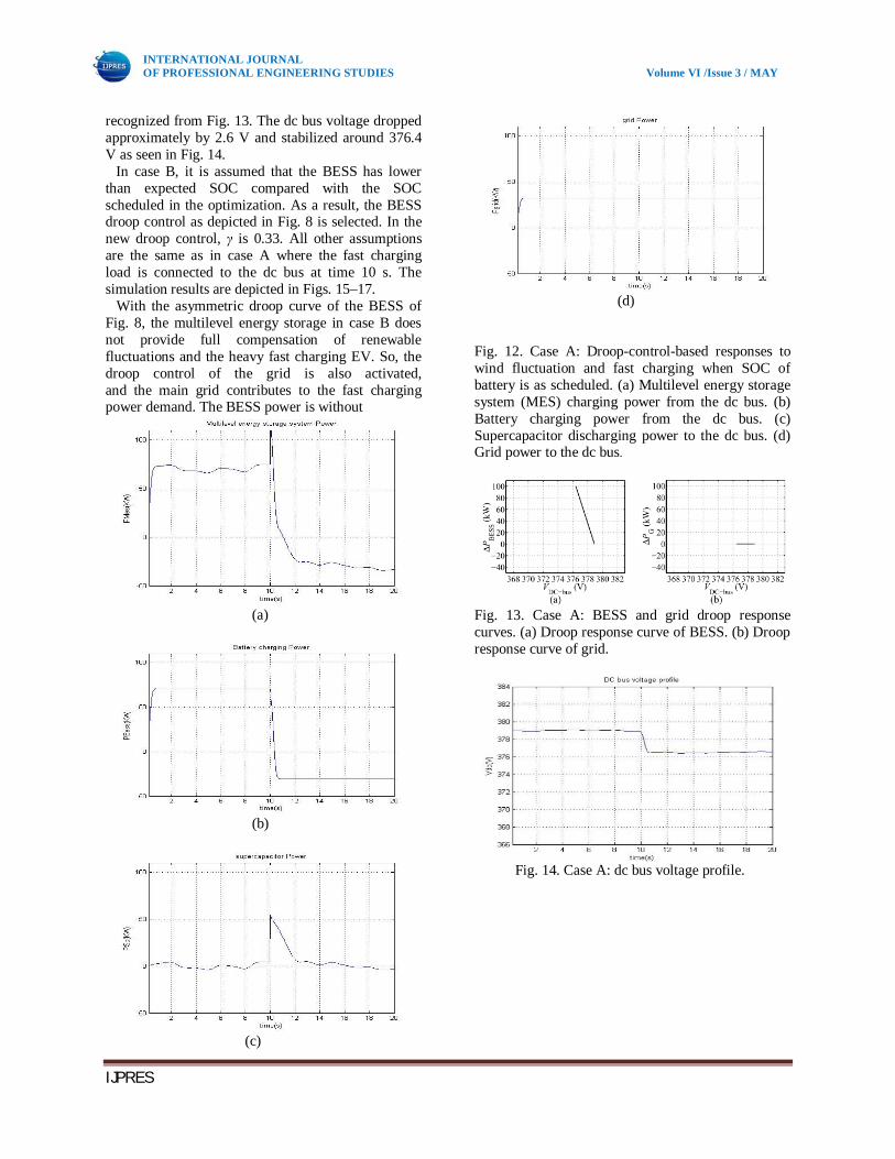
Fig. 11. Case study: Assumptions of the simulation. (a) Renewable power generation. (b) Fast charging load connected to the dc bus. For droop control of the BESS converter in normal SOC of the BESS in Fig. 7, the following assumptions are made: 푉 = (380 ± 1) V, 푉 = (380 ± 6) V, and 푃 = 200 kW. The BESS converter droop is set to react on voltage deviations higher than 1 V, and deviations below that value are neglected. The BESS converter power reaches its maximum change at dc bus voltage deviations of 6 V and higher. The main grid converter droop settings are assumed as follows: VGm1 = (380 ± 5) V, VGm2 = (380 ± 10) V, and maximum grid power is 300 kW. The voltage margins for the droop control of the grid converter are coordinated with the voltage margins for the droop control of the BESS converter in order to achieve the priority of BESS participation in controlling the voltage of the dc bus. Alternative approaches for coordinated droop controls of the converters may be found depending on the objective of the operation. In case A, it is assumed that the SOC of the battery is within close range of the scheduled SOC resulting from the day-ahead optimization. Therefore, the droop control in normal SOC of the battery as depicted in Fig. 7 is employed. The simulation results are shown in Figs. 12–14. The power PMES delivered by the multilevel energy storage combination of BESS and supercapacitor compensates both fast changes of renewable fluctuations and load. The rapid decrease of − PMES at 10 s shows that power is made readily available for fast charging. Thanks to the supercapacitor as cache energy storage, the power fluctuations do not propagate to the main grid. The grid power to the dc bus is unchanged. The droop control of the main grid converter is not active, and thus the grid power remains the same as scheduled. The functionality of the BESS droop control can be

INTERNATIONAL JOURNAL OF PROFESSIONAL ENGINEERING STUDIES Volume VI /Issue 3 / MAY 2016

IJPRES

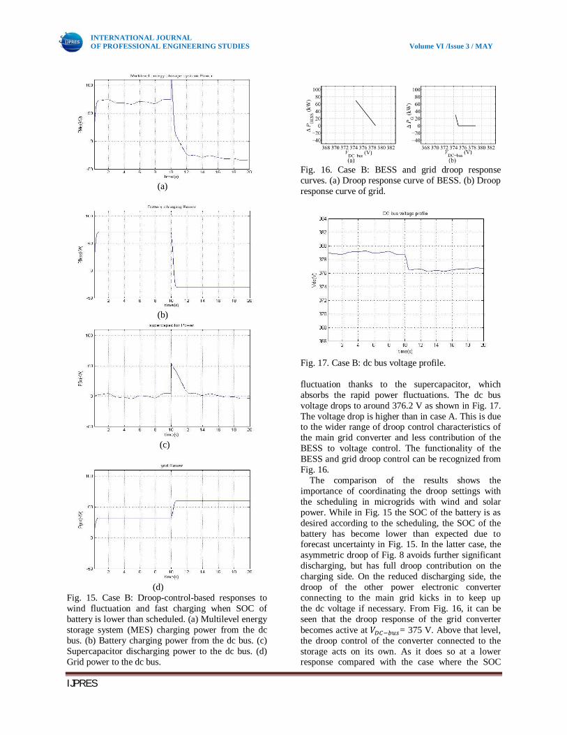
recognized from Fig. 13. The dc bus voltage dropped approximately by 2.6 V and stabilized around 376.4 V as seen in Fig. 14. In case B, it is assumed that the BESS has lower than expected SOC compared with the SOC scheduled in the optimization. As a result, the BESS droop control as depicted in Fig. 8 is selected. In the new droop control, γ is 0.33. All other assumptions are the same as in case A where the fast charging load is connected to the dc bus at time 10 s. The simulation results are depicted in Figs. 15–17. With the asymmetric droop curve of the BESS of Fig. 8, the multilevel energy storage in case B does not provide full compensation of renewable fluctuations and the heavy fast charging EV. So, the droop control of the grid is also activated, and the main grid contributes to the fast charging power demand. The BESS power is without

(a)

(b)

(c)

(d) Fig. 12. Case A: Droop-control-based responses to wind fluctuation and fast charging when SOC of battery is as scheduled. (a) Multilevel energy storage system (MES) charging power from the dc bus. (b) Battery charging power from the dc bus. (c) Supercapacitor discharging power to the dc bus. (d) Grid power to the dc bus.

Fig. 13. Case A: BESS and grid droop response curves. (a) Droop response curve of BESS. (b) Droop response curve of grid.

Fig. 14. Case A: dc bus voltage profile.

INTERNATIONAL JOURNAL OF PROFESSIONAL ENGINEERING STUDIES Volume VI /Issue 3 / MAY 2016

IJPRES

(a)

(b)

(c)

(d) Fig. 15. Case B: Droop-control-based responses to wind fluctuation and fast charging when SOC of battery is lower than scheduled. (a) Multilevel energy storage system (MES) charging power from the dc bus. (b) Battery charging power from the dc bus. (c) Supercapacitor discharging power to the dc bus. (d) Grid power to the dc bus.

Fig. 16. Case B: BESS and grid droop response curves. (a) Droop response curve of BESS. (b) Droop response curve of grid.

Fig. 17. Case B: dc bus voltage profile. fluctuation thanks to the supercapacitor, which absorbs the rapid power fluctuations. The dc bus voltage drops to around 376.2 V as shown in Fig. 17. The voltage drop is higher than in case A. This is due to the wider range of droop control characteristics of the main grid converter and less contribution of the BESS to voltage control. The functionality of the BESS and grid droop control can be recognized from Fig. 16. The comparison of the results shows the importance of coordinating the droop settings with the scheduling in microgrids with wind and solar power. While in Fig. 15 the SOC of the battery is as desired according to the scheduling, the SOC of the battery has become lower than expected due to forecast uncertainty in Fig. 15. In the latter case, the asymmetric droop of Fig. 8 avoids further significant discharging, but has full droop contribution on the charging side. On the reduced discharging side, the droop of the other power electronic converter connecting to the main grid kicks in to keep up the dc voltage if necessary. From Fig. 16, it can be seen that the droop response of the grid converter becomes active at 푉 = 375 V. Above that level, the droop control of the converter connected to the storage acts on its own. As it does so at a lower response compared with the case where the SOC

INTERNATIONAL JOURNAL OF PROFESSIONAL ENGINEERING STUDIES Volume VI /Issue 3 / MAY 2016

IJPRES

is not below the scheduled level, the steady-state ripple of VDC-bus in the first 10 s is higher in Fig. 17 than it is in Fig. 15. VI. CONCLUSION The renewable power which can be produced from the renewable resources can be integrated by the accumulated model. By this accumulated model the power for the individual time can be calculated. At particular time, the load will be connected to the dc bus. The renewable power will be served to the load through dc bus. If there is any uncertainty affiliated with the forecast of aggregated wind and pv based power generation was created and used to quantify the energy reserve of the battery energy storage system. The battery is parallel connected with the super capacitor to form multi level energy storage. The battery plays critical role for compensating the power fluctuations. The control proposed is here adaptive droop control in that the voltage-power droop curves are modified depending on the outcome of operational optimization. These voltage-power droop curves satisfy the load forecast uncertainties. The resulting energy system serves local stationary and ev based mobile consumers, and it is a good citizen within the main gird as it reduces emission by local usage of wind and solar energy.

REFERENCES [1] “Global wind report: Annual market update 2012,” Global Wind Energy Council, Brussels, Belgium, Tech. Rep., 2012. [2] H. Polinder, J. A. Ferreira, B. B. Jensen, A. B. Abrahamsen, K. Atallah, and R. A. McMahon, “Trends in wind turbine generator systems,” IEEE J. Emerg. Sel. Topics Power Electron., vol. 1, no. 3, pp. 174–185, Sep. 2013. [3] F. Giraud and Z. M. Salameh, “Steady-state performance of a gridconnected rooftop hybrid wind-photovoltaic power system with battery storage,” IEEE Trans. Energy Convers., vol. 16, no. 1, pp. 1–7, Mar. 2001. [4] B. S. Borowy and Z. M. Salameh, “Methodology for optimally sizing the combination of a battery bank and PV array in a wind/PV hybrid system,” IEEE Trans. Energy Convers., vol. 11, no. 2, pp. 367–375, Mar. 1996. [5] M. Cheng, S. Kato, H. Sumitani, and R. Shimada, “Flywheel-based AC cache power for stand-alone power systems,” IEEJ Trans. Electr. Electron. Eng., vol. 8, no. 3, pp. 290–296, May 2013. [6] H. Louie and K. Strunz, “Superconducting magnetic energy storage (SMES) for energy cache control in modular distributed hydrogenelectric

energy systems,” IEEE Trans. Appl. Supercond., vol. 17, no. 2, pp. 2361–2364, Jun. 2007. [7] A. L. Dimeas and N. D. Hatziargyriou, “Operation of a multiagent system for microgrid control,” IEEE Trans. Power Syst., vol. 20, no. 3, pp. 1447–1455, Aug. 2005. [8] F. Katiraei and M. R. Iravani, “Power management strategies for a microgrid with multiple distributed generation units,” IEEE Trans. Power Syst., vol. 21, no. 4, pp. 1821–1831, Nov. 2006. [9] A. G. Madureira and J. A. Pecas Lopes, “Coordinated voltage support in distribution networks with distributed generation and microgrids,” IET Renew. Power Generat., vol. 3, no. 4, pp. 439–454, Dec. 2009. [10] M. H. Nehrir, C. Wang, K. Strunz, H. Aki, R. Ramakumar, J. Bing,et al., “A review of hybrid renewable/alternative energy systems forelectric power generation: Configurations, control, and applications,”IEEE Trans. Sustain. Energy, vol. 2, no. 4, pp. 392–403, Oct. 2011. [11] R. Majumder, B. Chaudhuri, A. Ghosh, R. Majumder, G. Ledwich, and F. Zare, “Improvement of stability and load sharing in an autonomous microgrid using supplementary droop control loop,” IEEE Trans. Power Syst., vol. 25, no. 2, pp. 796–808, May 2010. [12] D. Westermann, S. Nicolai, and P. Bretschneider, “Energy management for distribution networks with storage systems—A hierarchical approach,” in Proc. IEEE PES General Meeting, Convers. Del. Electr. Energy 21st Century, Pittsburgh, PA, USA, Jul. 2008. [13] A. Chaouachi, R. M. Kamel, R. Andoulsi, and K. Nagasaka, “Multiobjective intelligent energy management for a microgrid,” IEEE Trans.Ind. Electron., vol. 60, no. 4, pp. 1688–1699, Apr. 2013. [14] R. Palma-Behnke, C. Benavides, F. Lanas, B. Severino, L. Reyes, J. Llanos, et al., “A microgrid energy management system based on the rolling horizon strategy,” IEEE Trans. Smart Grid, vol. 4, no. 2,pp. 996–1006, Jun. 2013. [15] R. Dai and M. Mesbahi, “Optimal power generation and load management for off-grid hybrid power systems with renewable sources via mixed-integer programming,” Energy Convers. Manag., vol. 73,pp. 234–244, Sep. 2013. [16] H. Kakigano, Y. Miura, and T. Ise, “Low-voltage bipolar-type DC microgrid for super high quality distribution,” IEEE Trans. Power Electron., vol. 25, no. 12, pp. 3066–3075, Dec. 2010. [17] D. Chen, L. Xu, and L. Yao, “DC voltage variation based autonomous control of DC microgrids,” IEEE Trans. Power Del., vol. 28, no. 2, pp. 637–648, Apr. 2013.

INTERNATIONAL JOURNAL OF PROFESSIONAL ENGINEERING STUDIES Volume VI /Issue 3 / MAY 2016

IJPRES

[18] L. Roggia, L. Schuch, J. E. Baggio, C. Rech, and J. R. Pinheiro, “Integrated full-bridge-forward DC-DC converter for a residential microgrid application,” IEEE Trans. Power Electron., vol. 28, no. 4, pp. 1728–1740, Apr. 2013. [19] K. Strunz and H. Louie, “Cache energy control for storage: Power system integration and education based on analogies derived from computer engineering,” IEEE Trans. Power Syst., vol. 24, no. 1, pp. 12–19, Feb. 2009. [20] “EMTDC transient analysis for PSCAD power system simulation version 4.2.0,” Manitoba HVDC Research Centre, Winnipeg, MB, Canada, Tech. Rep., 2005. [21] “Carbon dioxide emissions from the generation of electric power in the United States,” Dept. Energy, Environmental Protection Agency, Washington, DC, USA, Tech. Rep., 2000. [22] A. Yazdani and R. Iravani, Voltage-Sourced Converters in Power Systems. New York, NY, USA: Wiley, 2010. [23] E. Tara, S. Filizadeh, J. Jatskevich, E. Dirks, A. Davoudi, M. Saeedifard, et al., “Dynamic average-value modeling of hybrid-electric vehicular power systems,” IEEE Trans. Power Del., vol. 27, no. 1, pp. 430–438, Jan. 2012. Authors Profile:

M.Bala Jyothi pursuing M.Tech in Eluru College Of Engineering and Technology, Eluru.Her Specialization in Power Electronics.She graduated in Electrical and Electronics Engineering in Sri Vasavi Engineering College,Tadepalligudem affliated to JNTU Kakinada.

Mr.N.Phani Kumar, has obtained Eluru College Of Engineering and Technology, Eluru his M.Tech, Presently working as Asst. Professor in

Eluru College Of Engineering and Technology, Eluru,Affiliated to JNTU Kakinada