Embed Size (px)
Citation preview
City University of New York (CUNY) City University of New York (CUNY)
CUNY Academic Works CUNY Academic Works
Dissertations, Theses, and Capstone Projects CUNY Graduate Center
2-2019
Control of Energy Transfer and Molecular Energetics using Control of Energy Transfer and Molecular Energetics using
Photonic Nanostructures Photonic Nanostructures
Rahul Deshmukh The Graduate Center, City University of New York
How does access to this work benefit you? Let us know!
More information about this work at: https://academicworks.cuny.edu/gc_etds/3055
Discover additional works at: https://academicworks.cuny.edu
This work is made publicly available by the City University of New York (CUNY). Contact: [email protected]

1
Control of Energy Transfer and Molecular
Energetics using Photonic Nanostructures
by
Rahul Deshmukh
A dissertation submitted to the Graduate Faculty in Physics
in partial fulfillment of the requirements for the degree of
Doctor of Philosophy, The City University of New York
2019

ii
© 2019
Rahul Deshmukh
All rights reserved
iii
Control of Energy Transfer and Molecular Energetics using Photonic Nanostructures
by
Rahul Deshmukh
This manuscript has been read and accepted for the Graduate Faculty in Physics in satisfaction of
the dissertation requirement for the degree of Doctor of Philosophy.
Date Vinod M. Menon
Chair of Examining Committee
Date Sultan Catto
Executive Officer
Supervisory Committee:
Adam Braunschweig
Swapan Gayen
Neepa Maitra
Jacob Trevino
Joel Yuen Zhou
THE CITY UNIVERSITY OF NEW YORK

iv
ABSTRACT
Control of Energy Transfer and Molecular Energetics using Photonics Nanostructures
By
Rahul Deshmukh
In the last three decades, the design and fabrication of different types of photonic nanostructures
have allowed us to control and enhance the interaction of light (or photons) with matter (or
excitons). In this work, we demonstrate the use of three different nanostructures to control different
material properties. The design and fabrication of the nanostructures is discussed along with the
results obtained using characterization techniques of angle-resolved white light reflectivity and
transmission, and time-resolved and steady-state photoluminescence experiments. Specifically, we
demonstrate the use of Optical Topological Transitions (OTT) in metamaterials to show enhanced
efficiency in the non-radiative transfer of energy between two sets of molecules where the
separation is an order of magnitude higher than the traditional limit beyond which the energy
transfer is usually too small to be observed. We also utilize “strong coupling” : a regime of light-
matter interaction that results in the formation of part-light, part-matter quasi-particles and new
energy eigen states. This phenomenon in exploited in two cases. In the first, we demonstrate strong
coupling of an organic molecule, 3-(dimethylamino)-1-(2-hydroxy-4-methoxyphenyl)-2-propen-
1-one (HMPP), to a microcavity which results in modified dynamics of Excited State
Intramolecular Proton Transport (ESIPT) in HMPP. In the second case, we strongly couple
multiple vibronic transitions in another organic molecule, diindenoperylene (DIP), to surface
plasmons and demonstrate the resulting changes in emission properties at different temperatures.
v
ACKNOWLEDGEMENTS
First and foremost, I would like to thank my advisor, Prof. Vinod Menon for providing me the
opportunity to grow and learn in his research group. His constant enthusiasm for research and
relentless energy always inspires me. I have welcomed his frank feedback and his moral support
during some difficult times over the course of my PhD has been invaluable. I also enjoyed our
conversations about football (soccer), and music and food destinations in New York City. I would
also like to thank the other thesis committee members for their feedback and Daniel Moy in the
Physics Department office at the Graduate Center for his administrative help.
The same spirit of welcome camaraderie flows through the whole lab group, including the graduate
and undergraduate students, post docs and alumni, and I have made friends and enjoyed working
with them all. Special thanks are due to LaNMP alumnus Harish Krishnamoorthy, who I met
during a conference in India and whose talk introduced me to the group. I would also like to thank
Tal Galfsky who helped train me on various fabrication processes and collaborated on my first
project, on metamaterials. The post docs, Xiaoze Liu, Jared Day and Zav Shotan were very
helpful with keeping me focused and on track and were always available for questions and
explaining concepts. I would, however, advise caution while learning skiing with Zav. Deanna
Lombardo indulged my sweet tooth on several occasions with pies and cookies and was a
valuable, funny ally in the tedium of long grading and fabrication sessions. Nicholas Proscia was
my default roommate for most conferences and sounding board for new restaurants to explore. He
also was another valuable ally during the late-night experiment sessions. I will always have very
fond memories of Jie Gu, who helped make the lab a very pleasant place to be with his ready smile
and dedication for ‘beautiful’ research. In later years, I enjoyed the company of Zheng Sun, post
docs Biswanath Chakraborty and Sriram Guddala, and Mandeep Khatoniar. Other LaNMP
vi
members to be thanked include, in no particular order, Ryan Considine, Charles Cohen, Mike
Dollar, Rezlind Bushati, Sahana Das Bhattacharya, Emaad Khwaja, Alex Boehmke, Rian
Koots, Mohammed Hassan, Rong Wu, Paulo Marques and Dr. Divya K. Emaad, Paulo and
Divya also collaborated on my projects on energy transfer across metamaterials, strong coupling
with surface plasmons and cavity optochemistry, respectively. Other collaborators to be
acknowledged include Dr. Anurag Panda from University of Michigan, Dr. Svend-Age Biehs
from Carl von Ossietzky Universität at Oldenburg, Germany, Prof. G. S. Agarwal, now at Texas
A&M University, Prof. George John from the Department of Chemistry at CCNY and Dr. Joel
Yuen Zhou at UC San Diego. I would also like to acknowledge the wonderful nanofabrication
facilities and staff at the CUNY Advanced Science Research Center.
More than five years spent in New York City cannot be made enjoyable without friends outside
the lab and for that I would like to thank my roommates over the years Kailash, Jay, and
Sukhmeet. Vignesh, a friend from middle school took me in when I first arrived in the United
States and made the transition feel seamless. Brian and Rachel introduced me to the wonderful
world of boardgames and were willing outlets for all my other geeky exploits discussing movies,
science fiction and tv series, where they far outstrip my pitiful knowledge. In Siddharth and
Charuta, I found not only close friends but also an invaluable support network and I thank them
for that. Also, my time here could not possibly have been the same were it not for the Ekhalikar,
Ekhelikar and the Pathakji families. You’ve become family and a home away from home.
My parents, Dr. Rajendra and Dr. Shubhada Deshmukh, never put me under any pressure to
choose a particular profession as a kid, something for which I’ll always be grateful. Along with
my brother Sameer, they’ve been a source of unconditional support. My partner and wife Shruti,
joined me in the United States even though she had no guarantees of work and nobody she knew

vii
in a new country, and always loved, believed in me and supported me. My deepest appreciation
goes to her. And lastly, to the city of New York, which was an unforgettable backdrop to my PhD
years in all its busy, chaotic, dirty, smelly, beautiful and awe-inspiring glory.
viii
TABLE OF CONTENTS
ABSTRACT .................................................................................................................. iv
ACKNOWLEDGEMENTS .................................................................................................... v
TABLE OF CONTENTS .................................................................................................... viii
LIST OF FIGURES ........................................................................................................... x
1 Introduction .......................................................................................................... 1
2 Background ........................................................................................................... 5
2.1 Resonant Energy Transfer ............................................................................................................. 5
2.2 Examples of Photonic Nanostructures .......................................................................................... 6
2.2.1 Microcavities ......................................................................................................................... 7
2.2.2 Surface Plasmon Polaritons .................................................................................................. 8
2.2.3 Metamaterials ..................................................................................................................... 11
2.3 Regimes of light-matter interaction............................................................................................ 13
2.3.1 Classical treatment .............................................................................................................. 13
2.3.2 Quantum Mechanical treatment ........................................................................................ 15
2.3.3 A note on Ultra-strong coupling ......................................................................................... 17
2.4 Simulations .................................................................................................................................. 17
2.4.1 Transfer Matrix Method...................................................................................................... 17
2.4.2 Obtaining k and Kramers-Kronig relations .......................................................................... 19
3 Long Range Resonant Energy Transfer using Optical Topological Transitions in Metamaterials .... 21
3.1 Introduction ................................................................................................................................ 21
3.2 Metamaterial Design and Fabrication ........................................................................................ 23
3.3 Time-resolved and steady state experiments ............................................................................. 25
4 Modifying rate of Excited State Intramolecular Proton Transport using Cavity Ultra-Strong Coupling
30
4.1 Introduction ................................................................................................................................ 30
4.2 Sample fabrication and demonstration of strong coupling ........................................................ 31
4.3 Changes in emission trends ........................................................................................................ 35
5 Modification of photoluminescence spectra using strong coupling of vibronic transitions in organic
molecules with surface plasmons ..................................................................................... 40
5.1 Introduction ................................................................................................................................ 40
5.2 Experiment Design and Reflectivity ............................................................................................ 43
5.3 Photoluminescence modification ............................................................................................... 47
APPENDIX ................................................................................................................. 56

ix
A1. MATLAB code for calculating SPP dispersion based on Transfer Matrix Method. ........................ 56
A2. MATLAB code for Transfer Matrix Method (source code: Baruch Trazbonspor) ......................... 59
BIBLIOGRAPHY ........................................................................................................... 62
x
LIST OF FIGURES
Figure 2.1. Schematic representation of a microcavity with metallic mirrors. ................................ 7
Figure 2.2. Schematic representation of a surface plasmon polariton propagating along a metal –
dielectric interface. (Image Credit: Anil Thilsted) .................................................................. 8
Figure 2.3 Typical dispersion relation for surface plasmons in the ω-κ space. Image adapted with
permission from Scott T Parker. ........................................................................................ 9
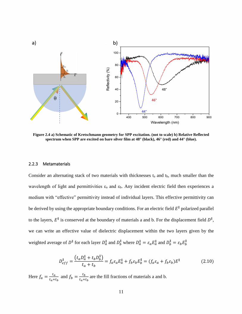
Figure 2.4 a) Schematic of Kretschmann geometry for SPP excitation. (not to scale) b) Relative
Reflected spectrum when SPP are excited on bare silver film at 48° (black), 46° (red) and 44° (blue). 11
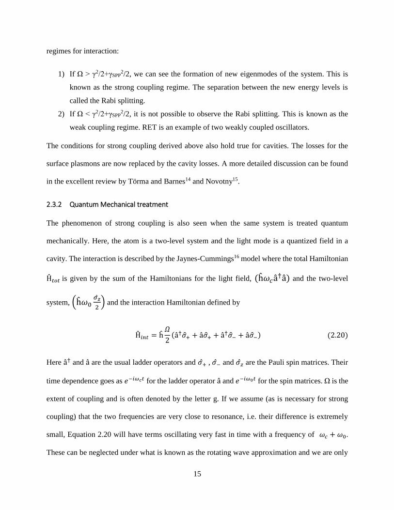
Figure 2.5. Schematic representation of a composite nanostructure with alternating subwavelength
layers. ..................................................................................................................... 12
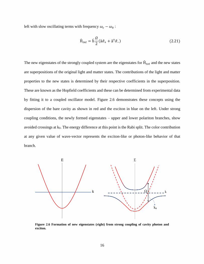
Figure 2.6 Formation of new eigenstates (right) from strong coupling of cavity photon and exciton. .. 16
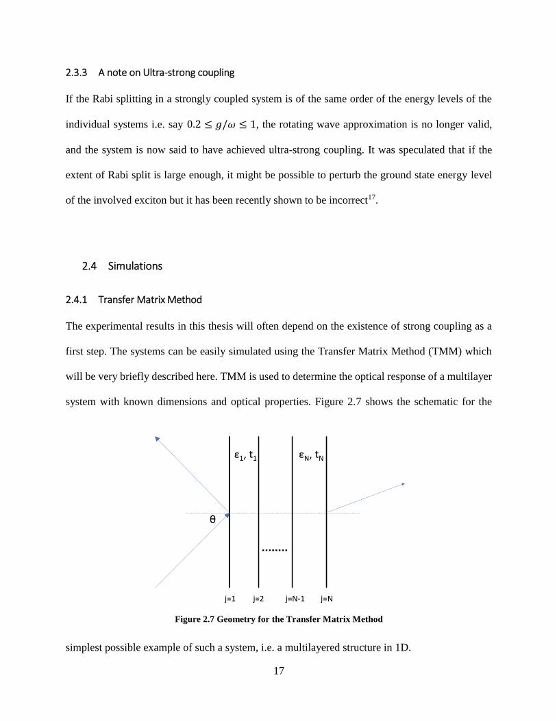
Figure 2.7 Geometry for the Transfer Matrix Method ............................................................. 17
Figure 2.8 Dispersion of SPP simulated using transfer matrix method (color plot) .......................... 19
Figure 3.1. Calculated Energy Transfer efficiency between dipoles oriented parallel and perpendicular
to the metamaterial. (*Image adapted from reference 23 with permission) ................................. 22
Figure 3.2. Sample design to demonstrate long range ET. ....................................................... 23
Figure 3.3. a) Effective medium theory calculations for a Ag/Al2O3 metamaterial with fill fraction 0.28.
b) TEM image of the cross-section of the metamaterial. ........................................................ 24
Figure 3.4. Donor lifetimes on glass (blue), on the metamaterial in the absence of acceptor (red) and
on the metamaterial in the presence of acceptor. ............................................................... 25
Figure 3.5 Donor lifetimes with (red) and without (black) acceptor in control samples where the DA pair
is separated by 160 nm of a) Silver and b) Al2O3 ................................................................... 26
Figure 3.7. a) Steady state emission collected in transmission mode showing increase in acceptor
emission. b) Difference of the two emission spectra (black) in a) superimposed on the acceptor
emission spectrum (red). .............................................................................................. 27
Figure 4.1 a) Tautomeric forms of HMPP. b) Absorption (black) and emission (red) spectra for HMPP in a
PMMA matrix. c) Cartoon showing the ESIPT process and the attempted change. .......................... 32
xi
Figure 4.2 Transmission measurements for HMPP in a cavity showing examples of a) weak coupling, b)
Strong coupling and c) Ultra strong coupling. ...................................................................... 33
Figure 4.3. Dispersion for the polariton branches for all the different concentrations of HMPP inside a
cavity ...................................................................................................................... 34
Figure 4.4 Steady PL spectra from strongly coupled samples collected at normal angle. ................. 35
Figure 4.5 Comparison of emission from HMPP inside the cavity (black squares) vs control sample
without cavity (red circles) ............................................................................................ 36
Figure 4.6. Total intensity of emission detected at normal collection vs concentration of HMPP in
cavities. ................................................................................................................... 37
Figure 4.7 Emission from 6mg/0.5mL HMPP in cavities centered at different redshifted wavelengths . 38
Figure 5.1 Schematic of an energy level diagram showing vibronic transitions. (Image credit: Mark M.
Somoza. Usage under CC license.) ................................................................................... 41
Figure 5.2. Real (black) and imaginary (red) parts of refractive index of DIP in standing orientation. The
inset shows the structure of DIP. Data courtesy of the group of Prof. Stephen Forrest from University of
Michigan ................................................................................................................... 42
Figure 5.3 Schematic of Angle resolved reflection experiment for DIP on silver. ........................... 43
Figure 5.4 Angle resolved reflectivity data from 46º to 69º from 30nm DIP on Silver.. .................... 45
Figure 5.5 a) Dispersion data for the strongly coupled DIP sample overlaid on simulation results. b)
Same dispersion data now plotted in E vs kx.. ..................................................................... 46
Figure 5.6 Calculated Hopfield coefficients for the different polariton branches. ......................... 47
Figure 5.7 Schematic of techniques for Photoluminescence studies a) Leakage radiation collected
through prism into the far field. and b) Emission collected on the same side as directly excited
molecules. ................................................................................................................ 48
Figure 5.8 a) Emission collected through prism and TM polarizer. b) Same data presented as a function
of angle in color plot.. ................................................................................................. 49
Figure 5.9 a) Emission comparison between a control sample of bare DIP on Silicon substrate (blue) and
our strongly coupled sample of DIP on silver (red). b) Same comparison at 77K. ........................... 51
Figure 5.10 Temperature dependent photoluminescence spectra from a) control sample and b) strongly

xii
coupled sample. ......................................................................................................... 53
Figure 5.11 Pl spectra comparing the emission of a) 30nm and b) 3nm DIP on Silicon and Silver
substrates at 77K.. ...................................................................................................... 54
1
The world around us is immersed in the interaction of light with matter as evidenced by phenomena
such as light harvesting for energy production by plants, phytoplankton and some kinds of bacteria,
and conversion of light to electrical signals in the retinas of our eyes. Humans have relentlessly
kept pushing the boundaries of our understanding about these kinds of interactions to harness them
for use in technology. With advancements in technology, we now have the ability to fabricate
devices thinner than a millionth of a meter, which is of the same order of magnitude as the
wavelength of light. These advancements now allow us to design and control the response of light
upon interaction with such devices. Examples include nanoscale mirrors and cavities, ring
resonators, photonic crystals, surface plasmons, metallic lattices for engineering the local response,
and many others including the era of artificially designed materials called metamaterials which
demonstrate properties which cannot occur naturally. We collectively refer to these devices as
photonic nanostructures. Their ability to overcome diffraction limits and squeeze light into ever-
smaller dimensions with highly enhanced fields results in some extraordinary phenomena.
Interaction with materials capable of absorbing and emitting light is affected greatly and we begin
to observe the occurrence of new regimes of interaction which are not observed at macroscopic
levels.
The main theme of this work is to exploit the ability of photonic nanostructures to support these
1 Introduction
2
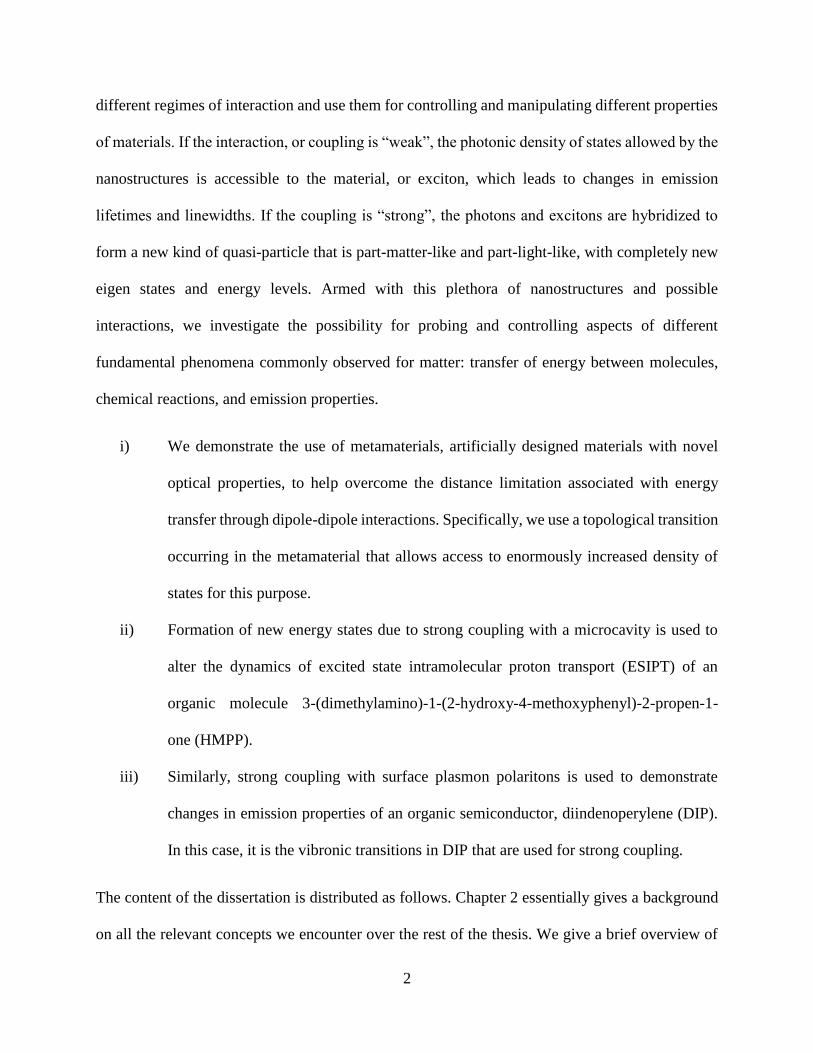
different regimes of interaction and use them for controlling and manipulating different properties
of materials. If the interaction, or coupling is “weak”, the photonic density of states allowed by the
nanostructures is accessible to the material, or exciton, which leads to changes in emission
lifetimes and linewidths. If the coupling is “strong”, the photons and excitons are hybridized to
form a new kind of quasi-particle that is part-matter-like and part-light-like, with completely new
eigen states and energy levels. Armed with this plethora of nanostructures and possible
interactions, we investigate the possibility for probing and controlling aspects of different
fundamental phenomena commonly observed for matter: transfer of energy between molecules,
chemical reactions, and emission properties.
i) We demonstrate the use of metamaterials, artificially designed materials with novel
optical properties, to help overcome the distance limitation associated with energy
transfer through dipole-dipole interactions. Specifically, we use a topological transition
occurring in the metamaterial that allows access to enormously increased density of
states for this purpose.
ii) Formation of new energy states due to strong coupling with a microcavity is used to
alter the dynamics of excited state intramolecular proton transport (ESIPT) of an
organic molecule 3-(dimethylamino)-1-(2-hydroxy-4-methoxyphenyl)-2-propen-1-
one (HMPP).
iii) Similarly, strong coupling with surface plasmon polaritons is used to demonstrate
changes in emission properties of an organic semiconductor, diindenoperylene (DIP).
In this case, it is the vibronic transitions in DIP that are used for strong coupling.
The content of the dissertation is distributed as follows. Chapter 2 essentially gives a background
on all the relevant concepts we encounter over the rest of the thesis. We give a brief overview of
3
all the photonic nanostructures that are used in the presented research – microcavities, surface
plasmons and metamaterials. The theoretical underpinnings of the behavior of the nanostructures
are discussed. We also introduce the topic of light-matter interactions in a little more detail, going
over the different possible regimes and the resultant general outcomes. We briefly discuss the
principles behind the simulations for expected response of the light-matter interaction. The
principles behind Resonance Energy Transfer (RET) are also discussed, which is one of the
properties that can be affected by light matter interaction.
In Chapter 3, we demonstrate the use of metamaterials to enhance the limit of RET. While this
process is fundamentally limited to occur within a range of ~10nm, we demonstrate an order of
magnitude increase over this distance over which we still observe the transfer of energy through
direct interactions. The design of the metamaterial required to show such an effect is discussed.
Evidence from time-resolved and steady state photoluminescence (PL) experiments is used to
support our claim of long-range energy transfer.
Next, we turn our attention to modifying material properties by the formation of hybrid particles
using strong coupling. In Chapter 4, we show ultra-strong coupling of a metallic cavity to an
organic molecule in order to investigate possible effects on its chemical transformations. A brief
overview of the transformation under question, ESIPT, is given. Change in emission trends of the
molecule HMPP in microcavities under strong and ultra-strong coupling are shown through
concentration dependent studies.
Finally, Chapter 5 describes the use of surface plasmon polaritons to change the
photoluminescence properties of an organic semiconductor dye, DIP, using strong coupling with
multiple vibronic transitions in DIP. The strong coupling is demonstrated using angle resolved
reflectivity. We also discuss the different possible configurations to be used for steady-state PL

4
studies and show the use of an uncommon configuration to observe changes in the PL spectra. The
changes come from redistribution of the spectral weights from each of the vibronic transitions
contributing to the total emission. This evolution of this redistribution is studied as a function of
temperature.
5
2.1 Resonant Energy Transfer
Resonance Energy Transfer (RET)1 is a process by which a molecule in its excited state (called
donor) transfers energy to another molecule (called acceptor) non-radiatively. It is the result of
direct interaction between the dipoles of the two molecules. If the transfer of energy happens
without any exchange of an electron, it is called the Förster Resonance Energy Transfer (FRET)2.
The rate of energy transfer depends on the extent of the spectral overlap of the emission spectrum
of the donor with the absorption spectrum of the acceptor, the orientations of the two dipoles, the
quantum yield of the donor, spontaneous emission lifetime of the donor and the distance between
the two molecules. Once a donor-acceptor (DA) pair and the experimental conditions have been
chosen, we can express the FRET rates by1,3
𝑘𝑇(𝑟) =1
𝜏𝐷(𝑅0
𝑟)6
(2.1)
where τD is the donor lifetime in the absence of acceptor and R0 is called the Förster Radius. R0 is
specific to a donor-acceptor pair and contains the dependence on spectral overlap, donor quantum
yield, and dipole orientation factor mentioned earlier. The strong distance dependence means that
RET is not observed beyond a DA separation of ~ 10-15nm.
If we consider donor molecules in their excited state, the total decay rate of the molecules to the
2 Background
6
ground state can be expressed as a sum of the radiative and non-radiative decay rates. When an
acceptor molecule is present at distances less than ~2R0, RET is enabled and the non-radiative
decay rates increase. Thus, by definition, the lifetime of the molecule (Time taken for the number
of molecules in excited states to reduce to 1/e of the original number) must decrease. If the acceptor
is emissive, then the emission intensity from the acceptor must increase. These are the two
conditions required to demonstrate RET. Once these are met, one can determine the ET efficiency
by
𝐸 = 1 −𝜏𝐷𝐴
𝜏𝐷 (2.2)
where τDA is the donor lifetime in the presence of acceptor.
Prominent examples of RET include its use in photosynthesis4,5, where the process is used to
efficiently transfer the energy of absorbed photons to the reaction centers present in a different
location. The distance dependence in RET can also be exploited for use as a molecular ruler in
structural biology4, where fluorescent markers are attached different biomolecules to deduce
folding patterns using the distance between the markers at different times. This same dependence
acts as a limitation in the scope of its use and it would be desirable to overcome this barrier in
RET. This would also help in man-made systems for solar harvesting6,7 and organic LED’s8.
2.2 Examples of Photonic Nanostructures
In this thesis, we will consider 3 different types of nanostructures: microcavities, surface plasmon
polaritons (SPPs) and metamaterials. In each case, the layer thicknesses are subwavelength.
7
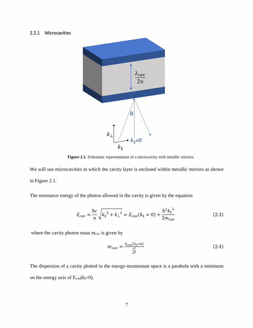
2.2.1 Microcavities
We will use microcavities in which the cavity layer is enclosed within metallic mirrors as shown
in Figure 2.1.
The resonance energy of the photon allowed in the cavity is given by the equation
𝐸𝑐𝑎𝑣 =ħ𝑐
𝑛√𝑘∥
2 + 𝑘⊥2 = 𝐸𝑐𝑎𝑣(𝑘∥ = 0) +
ħ2𝑘∥2
2𝑚𝑐𝑎𝑣 (2.3)
where the cavity photon mass mcav is given by
𝑚𝑐𝑎𝑣 =𝐸𝑐𝑎𝑣(𝑘∥=0)
𝑐2
𝑛2
(2.4)
The dispersion of a cavity plotted in the energy-momentum space is a parabola with a minimum
on the energy axis of Ecav(k∥=0).
Figure 2.1. Schematic representation of a microcavity with metallic mirrors.

8
2.2.2 Surface Plasmon Polaritons
Surface plasmons are quantized electron density oscillations localized at the interface of a metal
and a dielectric. We will follow the approach described by Novotny9 to describe the theory. The
expressions for the electric fields can be obtained by solving the wave equation
𝛻 × 𝛻 × 𝑬(𝒓, 𝜔) −𝜔2
𝑐2𝜀(𝒓, 𝜔)𝑬(𝒓,𝜔) = 0 (2.5)
for both sides of the interface. We look for solutions localized to the interface, i.e. decaying
exponentially away on both sides. This is only possible if we use the expressions for Transverse
Magnetic (TM) or p-polarized wave. Thus, the fields can be written as
𝐸𝑗 = (
𝐸𝑗,𝑥
0𝐸𝑗,𝑧
)𝑒𝑖𝑘𝑥𝑥𝑒−𝑖𝑘𝑗,𝑧|𝑧|𝑒−𝑖𝜔𝑡, 𝑗 = 1,2 (2.6)
where the values for j represent both sides of the interface. We can further use the Maxwell
Figure 2.2. Schematic representation of a surface plasmon polariton propagating along a metal – dielectric
interface. The exponential dependence of the electromagnetic field intensity on the distance away from the
interface is shown on the right. (Image Credit: Anil Thilsted)
9
Equation 𝛻 ⋅ 𝑫 = 0 along with the condition for continuity of parallel component of electric field
and perpendicular component of Displacement field at the interface and obtain
𝜀1
𝜀2= −
𝑘1,𝑧
𝑘2,𝑧 (2.7)
Since the wavevector parallel to the interface kx is conserved, we can use Equation 2.7 to obtain
the dispersion relation for surface plasmons
𝑘𝑥 =𝜔
𝑐√
𝜀1𝜀2
𝜀1 + 𝜀2
(2.8)
The components of wavevectors perpendicular to the interface are given by
𝑘𝑗,𝑧 =𝜔
𝑐
𝜀𝑗
√𝜀1 + 𝜀2
, 𝑗 = 1,2. (2.9)
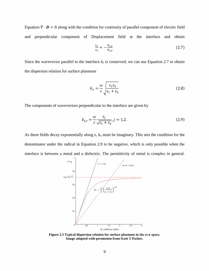
As these fields decay exponentially along z, kz must be imaginary. This sets the condition for the
denominator under the radical in Equation 2.9 to be negative, which is only possible when the
interface is between a metal and a dielectric. The permittivity of metal is complex in general.
Figure 2.3 Typical dispersion relation for surface plasmons in the ω-κ space.
Image adapted with permission from Scott T Parker.

10
Keeping this in mind, Equation 2.8 then describes the propagation of the wave along the interface
for a characteristic length before it gets absorbed by the metal. Equation 2.8 can also be used to
plot the dispersion relation for surface plasmons. Figure 2.3 shows the dispersion relation for an
arbitrarily chosen metal-dielectric interface. The straight line in blue depicts the light line for air,
i.e. the maximum possible wave vector allowed for a photon of a given energy. The dispersion of
the surface plasmons clearly lie below the light line, and thus it is not possible to excite them
plasmons directly from light incident from far field in air. For a given energy, we need a parallel
momentum higher than that of a photon in air. Thus, the incident light has to come through a higher
index material like a prism. A part of the shown dispersion would then lie above the light line for
the prism, again as shown in Figure 2.3 and these modes are now accessible. Since these modes
are coupled to the electromagnetic waves, they are also called the surface plasmon polaritons
(SPP). Another excellent source for detailed theory on SPPs is the monograph by Raether.10
A widely used method for the excitation of SPPs is the Kretschmann configuration11 in which there
is no separation between the metal film and the prism as shown in Figure 2.4a. The reflected light
is recorded relative to the incident white light at various angles. Wherever the required momentum
matching conditions are satisfied, the corresponding wavelengths are utilized in exciting the SPP
and show up as a dip in relative reflected intensity, as shown in Figure 2.4b.
11
2.2.3 Metamaterials
Consider an alternating stack of two materials with thicknesses ta and tb, much smaller than the
wavelength of light and permittivities εa and εb. Any incident electric field then experiences a
medium with “effective” permittivity instead of individual layers. This effective permittivity can
be derived by using the appropriate boundary conditions. For an electric field 𝐸∥ polarized parallel
to the layers, 𝐸∥ is conserved at the boundary of materials a and b. For the displacement field 𝐷∥,
we can write an effective value of dielectric displacement within the two layers given by the
weighted average of 𝐷∥ for each layer 𝐷𝑎∥ and 𝐷𝑏
∥ where 𝐷𝑎∥ = 𝜀𝑎𝐸𝑎
∥ and 𝐷𝑏∥ = 𝜀𝑏𝐸𝑏
∥
𝐷𝑒𝑓𝑓∥ =
(𝑡𝑎𝐷𝑎∥ + 𝑡𝑏𝐷𝑏
∥)
𝑡𝑎 + 𝑡𝑏= 𝑓𝑎𝜀𝑎𝐸𝑎
∥ + 𝑓𝑏𝜀𝑏𝐸𝑏∥ = (𝑓𝑎𝜀𝑎 + 𝑓𝑏𝜀𝑏)𝐸
∥ (2.10)
Here 𝑓𝑎 =𝑡𝑎
𝑡𝑎+𝑡𝑏 and 𝑓𝑏 =
𝑡𝑏
𝑡𝑎+𝑡𝑏 are the fill fractions of materials a and b.
Figure 2.4 a) Schematic of Kretschmann geometry for SPP excitation. (not to scale) b) Relative Reflected
spectrum when SPP are excited on bare silver film at 48° (black), 46° (red) and 44° (blue).

12
If we also express 𝐷𝑒𝑓𝑓∥ as 𝜀𝑒𝑓𝑓
∥ 𝐸𝑒𝑓𝑓∥ , then the effective permittivity reduces to
𝜀𝑒𝑓𝑓||
= 𝑓𝑎𝜀𝑎 + 𝑓𝑏𝜀𝑏 if field is polarized parallel to the layers (2.11)
Similarly, if we consider an electric field polarized perpendicular to the layers, the Displacement
field 𝐷⊥ is conserved at each interface. Following a similar derivation as earlier, we can easily
realize the equation
1
𝜀𝑒𝑓𝑓⊥ =
𝑓𝑎
𝜀𝑎+
𝑓𝑏
𝜀𝑏 if field is polarized normal to the layers (2.12)
Thus, we have an anisotropic material. The dispersion of the material in the energy-momentum
space can then be given by the iso-frequency surface:
𝑘𝑥2+𝑘𝑦
2
𝜀⊥+
𝑘𝑧2
𝜀||= 𝜔2/𝑐2 (2.13)
If both materials are dielectrics, ε⊥ and ε∥ are positive and the surface is just a regular ellipsoid.
Figure 2.5. Schematic representation of a composite nanostructure with alternating subwavelength layers.

13
However, if we choose one of the materials to be a metal, the fill fractions can be adjusted so that
one of the components of the permittivity becomes negative. In this case, when we plot ε∥ as a
function of wavelength/frequency, it changes from positive to zero to negative as the permittivity
of the metal starts becoming more and more negative. During this transition, the iso-frequency
contour changes from a closed ellipsoid to an open hyperboloid. This point is called an optical
topological transition12,13 and the alternating metal-dielectric stack is called a metamaterial. The
available photonic density of states, which is given by the volume enclosed by the iso-frequency
surface, is theoretically infinite. However, once losses are taken into account, this number becomes
finite but remains highly increased. This enormous increase in the density of states is now available
for any exciton present in the near field of the metamaterial.
2.3 Regimes of light-matter interaction
The interaction of light with matter can be classified broadly into two categories – weak and strong.
Theoretically, these can be derived both using either classical or quantum treatments. In this
section, we will briefly describe both.
2.3.1 Classical treatment
We specifically discuss the interaction of matter with SPPs here. The interaction with cavities
follows the same principles.
The expression for the permittivity of a medium can be easily derived using the Lorenz Drude
model and is given by:
𝜀(𝜔) = 1 + 𝜒(𝜔) (2.14)

14
Where χ(ω) is called the susceptibility and given by the equation:
𝜒(𝜔) =𝑁𝑒2
𝑉𝜀0𝑚
1
𝜔02−𝜔2−𝑖𝛾𝜔
(2.15)
We will use these expressions in equation 2.8 to describe the interaction of matter with Surface
plasmons. We assume that the permittivity of the metal is constant and a large negative value. The
permittivity of the other material (in this case, our interacting matter) is now described by the
general expressions for permittivity in Equations 2.13 and 2.14. Substituting the appropriate
values, we get a new equation for the dispersion:
𝜅2 = 𝜔2 (1 +𝛺
𝜔02−𝜔2−𝑖𝛾𝜔
) (2.16)
where κ is the new scaled momentum given by 𝜅2 = 𝑘2 𝑐2|𝜀1+𝜀2|
|𝜀1| and 𝛺 =
𝑁𝑒2
𝑉𝜀0𝑚 (2.17)
We can solve this equation near resonance i.e. under the conditions ω and κ are quite close to ω0:
𝜔± =𝜅
2+
𝜔0
2− 𝑖
𝛾
4±
1
2√𝛺 + (𝜅 − 𝜔0 + 𝑖𝛾/2)2 (2.18)
Here γ is a damping term that describes the material losses. We can also include the losses of the
surface plasmons γSPP by rewriting κ as (κ - iγSPP/2) in equation 2.18 and at resonance, we get the
solutions:
𝜔± = 𝜔0 − 𝑖𝛾
4− 𝑖
𝛾𝑆𝑃𝑃
4±
1
2√𝛺 − (
𝛾
2−
𝛾𝑆𝑃𝑃
2)2
(2.19)
We now seem to have the expressions for two new energy states ω+ and ω-. However, we will be
able to observe these modes in the ω-k plane only if the separation between them is greater than
the damping terms i.e. √𝛺 − (𝛾
2−
𝛾𝑆𝑃𝑃
2)2
>𝛾
2+
𝛾𝑆𝑃𝑃
2. This sets the condition for the different
15
regimes for interaction:
1) If Ω > γ2/2+γSPP2/2, we can see the formation of new eigenmodes of the system. This is
known as the strong coupling regime. The separation between the new energy levels is
called the Rabi splitting.
2) If Ω < γ2/2+γSPP2/2, it is not possible to observe the Rabi splitting. This is known as the
weak coupling regime. RET is an example of two weakly coupled oscillators.
The conditions for strong coupling derived above also hold true for cavities. The losses for the
surface plasmons are now replaced by the cavity losses. A more detailed discussion can be found
in the excellent review by Törma and Barnes14 and Novotny15.
2.3.2 Quantum Mechanical treatment
The phenomenon of strong coupling is also seen when the same system is treated quantum
mechanically. Here, the atom is a two-level system and the light mode is a quantized field in a
cavity. The interaction is described by the Jaynes-Cummings16 model where the total Hamiltonian
Ĥ𝑡𝑜𝑡 is given by the sum of the Hamiltonians for the light field, (ĥ𝜔𝑐â†â) and the two-level
system, (ĥ𝜔0𝜎̂ 𝑧
2) and the interaction Hamiltonian defined by
Ĥ𝑖𝑛𝑡 = ĥ𝛺
2(â†�̂�+ + â�̂�+ + â†�̂�− + â�̂�−) (2.20)
Here ↠and â are the usual ladder operators and 𝜎 + , 𝜎 − and 𝜎 𝑧 are the Pauli spin matrices. Their
time dependence goes as 𝑒−𝑖𝜔𝑐𝑡 for the ladder operator â and 𝑒−𝑖𝜔0𝑡 for the spin matrices. Ω is the
extent of coupling and is often denoted by the letter g. If we assume (as is necessary for strong
coupling) that the two frequencies are very close to resonance, i.e. their difference is extremely
small, Equation 2.20 will have terms oscillating very fast in time with a frequency of 𝜔𝑐 + 𝜔0.
These can be neglected under what is known as the rotating wave approximation and we are only
16
left with slow oscillating terms with frequency 𝜔𝑐 − 𝜔0 :
Ĥ𝑖𝑛𝑡 = ĥ𝛺
2(â�̂�+ + â†�̂�−) (2.21)
The new eigenstates of the strongly coupled system are the eigenstates for Ĥ𝑡𝑜𝑡 and the new states
are superpositions of the original light and matter states. The contributions of the light and matter
properties to the new states is determined by their respective coefficients in the superposition.
These are known as the Hopfield coefficients and these can be determined from experimental data
by fitting it to a coupled oscillator model. Figure 2.6 demonstrates these concepts using the
dispersion of the bare cavity as shown in red and the exciton in blue on the left. Under strong
coupling conditions, the newly formed eigenstates – upper and lower polariton branches, show
avoided crossings at k0. The energy difference at this point is the Rabi split. The color contribution
at any given value of wave-vector represents the exciton-like or photon-like behavior of that
branch.
Figure 2.6 Formation of new eigenstates (right) from strong coupling of cavity photon and
exciton.
17
2.3.3 A note on Ultra-strong coupling
If the Rabi splitting in a strongly coupled system is of the same order of the energy levels of the
individual systems i.e. say 0.2 ≤ 𝑔/𝜔 ≤ 1, the rotating wave approximation is no longer valid,
and the system is now said to have achieved ultra-strong coupling. It was speculated that if the
extent of Rabi split is large enough, it might be possible to perturb the ground state energy level
of the involved exciton but it has been recently shown to be incorrect17.
2.4 Simulations
2.4.1 Transfer Matrix Method
The experimental results in this thesis will often depend on the existence of strong coupling as a
first step. The systems can be easily simulated using the Transfer Matrix Method (TMM) which
will be very briefly described here. TMM is used to determine the optical response of a multilayer
system with known dimensions and optical properties. Figure 2.7 shows the schematic for the
simplest possible example of such a system, i.e. a multilayered structure in 1D.
Figure 2.7 Geometry for the Transfer Matrix Method
18
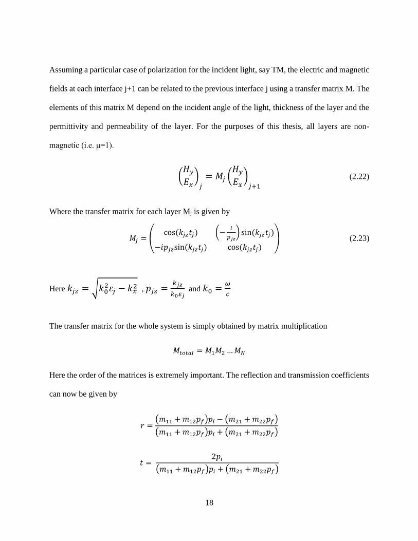
Assuming a particular case of polarization for the incident light, say TM, the electric and magnetic
fields at each interface j+1 can be related to the previous interface j using a transfer matrix M. The
elements of this matrix M depend on the incident angle of the light, thickness of the layer and the
permittivity and permeability of the layer. For the purposes of this thesis, all layers are non-
magnetic (i.e. μ=1).
(𝐻𝑦
𝐸𝑥)𝑗
= 𝑀𝑗 (𝐻𝑦
𝐸𝑥)𝑗+1
(2.22)
Where the transfer matrix for each layer Mj is given by
𝑀𝑗 = (cos (𝑘𝑗𝑧𝑡𝑗) (−
𝑖
𝑝𝑗𝑧) sin (𝑘𝑗𝑧𝑡𝑗)
−𝑖𝑝𝑗𝑧sin (𝑘𝑗𝑧𝑡𝑗) cos (𝑘𝑗𝑧𝑡𝑗)) (2.23)
Here 𝑘𝑗𝑧 = √𝑘02𝜀𝑗 − 𝑘𝑥
2 , 𝑝𝑗𝑧 =𝑘𝑗𝑧
𝑘0𝜀𝑗 and 𝑘0 =
𝜔
𝑐
The transfer matrix for the whole system is simply obtained by matrix multiplication
𝑀𝑡𝑜𝑡𝑎𝑙 = 𝑀1𝑀2 …𝑀𝑁
Here the order of the matrices is extremely important. The reflection and transmission coefficients
can now be given by
𝑟 =(𝑚11 + 𝑚12𝑝𝑓)𝑝𝑖 − (𝑚21 + 𝑚22𝑝𝑓)
(𝑚11 + 𝑚12𝑝𝑓)𝑝𝑖 + (𝑚21 + 𝑚22𝑝𝑓)
𝑡 = 2𝑝𝑖
(𝑚11 + 𝑚12𝑝𝑓)𝑝𝑖 + (𝑚21 + 𝑚22𝑝𝑓)
19
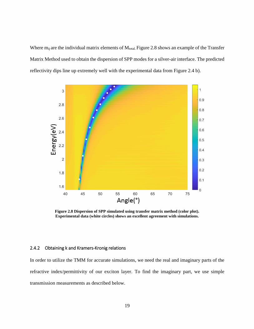
Where mij are the individual matrix elements of Mtotal. Figure 2.8 shows an example of the Transfer
Matrix Method used to obtain the dispersion of SPP modes for a silver-air interface. The predicted
reflectivity dips line up extremely well with the experimental data from Figure 2.4 b).
2.4.2 Obtaining k and Kramers-Kronig relations
In order to utilize the TMM for accurate simulations, we need the real and imaginary parts of the
refractive index/permittivity of our exciton layer. To find the imaginary part, we use simple
transmission measurements as described below.
Figure 2.8 Dispersion of SPP simulated using transfer matrix method (color plot).
Experimental data (white circles) shows an excellent agreement with simulations.
20
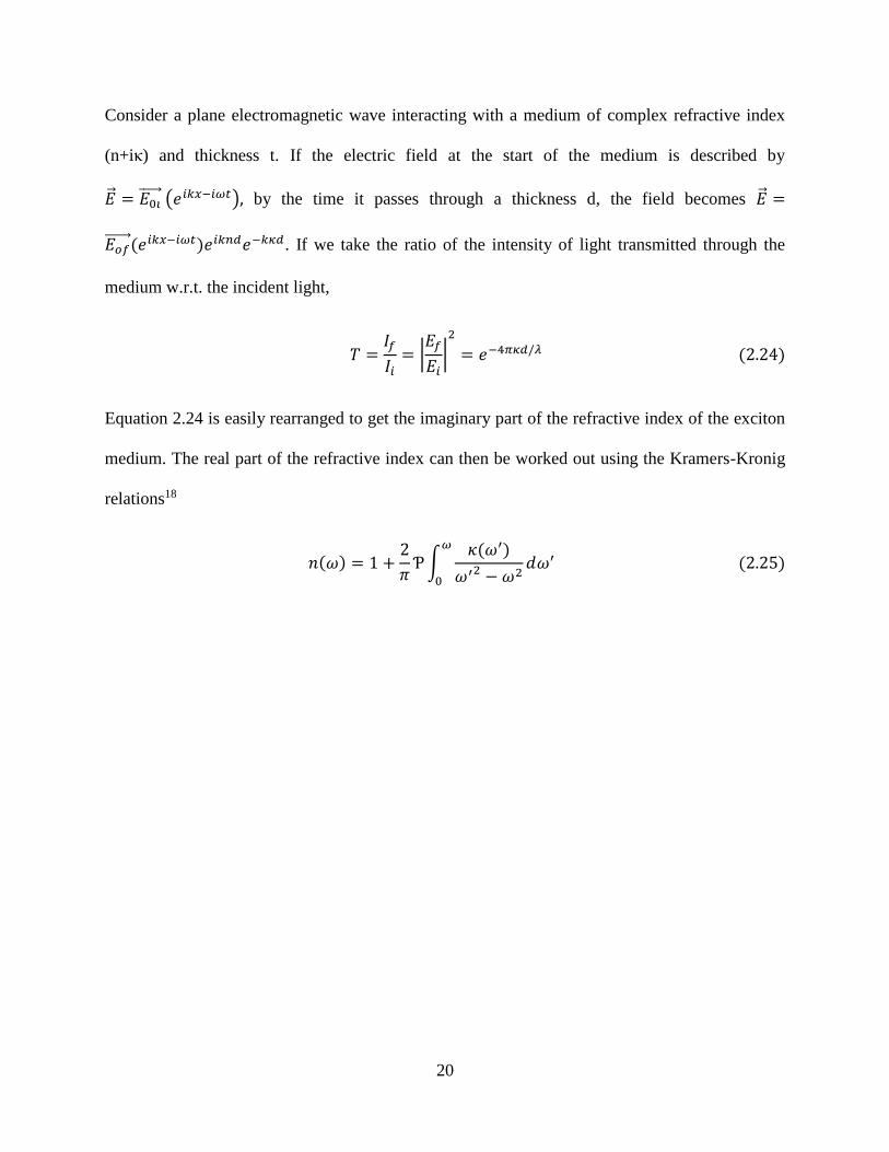
Consider a plane electromagnetic wave interacting with a medium of complex refractive index
(n+iκ) and thickness t. If the electric field at the start of the medium is described by
�⃗� = 𝐸0𝑖⃗⃗ ⃗⃗ ⃗ (𝑒𝑖𝑘𝑥−𝑖𝜔𝑡), by the time it passes through a thickness d, the field becomes �⃗� =
𝐸𝑜𝑓⃗⃗ ⃗⃗ ⃗⃗ (𝑒𝑖𝑘𝑥−𝑖𝜔𝑡)𝑒𝑖𝑘𝑛𝑑𝑒−𝑘𝜅𝑑. If we take the ratio of the intensity of light transmitted through the
medium w.r.t. the incident light,
𝑇 =𝐼𝑓
𝐼𝑖= |
𝐸𝑓
𝐸𝑖|2
= 𝑒−4𝜋𝜅𝑑/𝜆 (2.24)
Equation 2.24 is easily rearranged to get the imaginary part of the refractive index of the exciton
medium. The real part of the refractive index can then be worked out using the Kramers-Kronig
relations18
𝑛(𝜔) = 1 +2
𝜋Ƥ∫
𝜅(𝜔′)
𝜔′2 − 𝜔2𝑑𝜔′
𝜔
0
(2.25)

21
3.1 Introduction
We discussed earlier in Chapters 1 and 2 about the motivation behind improving the efficiency of
the Resonance Energy Transfer (RET) process using various photonic nanostructures. Indeed,
there have been several efforts in this direction, starting with experiments by Andrew and Barnes19
in 2000, where they demonstrated experimentally that the FRET process can be controlled by the
local density of states in a microcavity. They followed this by showing ET at a donor-acceptor
separation of 120 nm across a silver film in 200420 but were unable to conclude if the ET was non-
radiative. These demonstrations paved the way for several other groups to demonstrate long-range
ET assisted by surface plasmon polaritons (SPPs), as seen in the work by Martin-Cano et. al21, de
Torres et. al22. and Bouchet23 et. al. In each of these, ET was demonstrated across a separation of
the order of microns. However, these demonstrations come with the caveat that they were assisted
by the propagating SPPs and thus aren’t true examples of resonant dipole-dipole interactions.
Theoretical works by Ren et. al.24 showed that it might indeed be possible to achieve enhanced
FRET using donor/acceptors at plasmonic hotspots. But the work of Biehs25 et. al. was most
promising, where they theorized that an optimal medium to show FRET rate and efficiency
enhancements could be hyperbolic metamaterials, specifically the points of optical topological
transitions where it is possible to exploit the enormous increase in the Local Density of States
3 Long Range Resonant Energy Transfer using Optical Topological
Transitions in Metamaterials
22
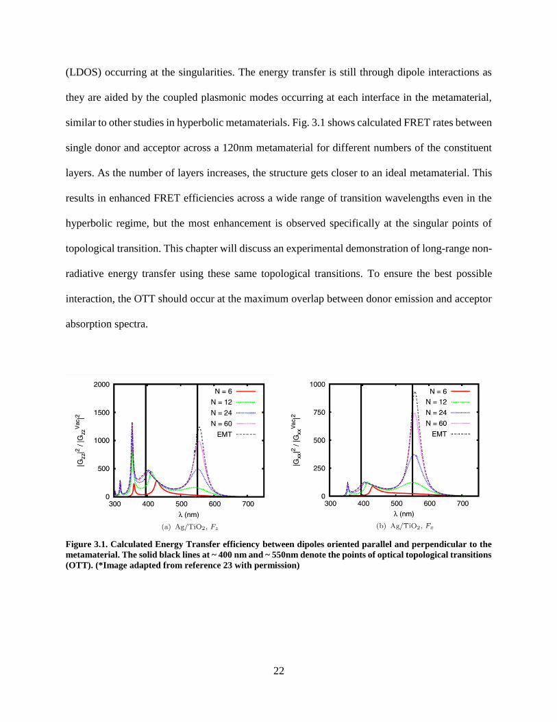
(LDOS) occurring at the singularities. The energy transfer is still through dipole interactions as
they are aided by the coupled plasmonic modes occurring at each interface in the metamaterial,
similar to other studies in hyperbolic metamaterials. Fig. 3.1 shows calculated FRET rates between
single donor and acceptor across a 120nm metamaterial for different numbers of the constituent
layers. As the number of layers increases, the structure gets closer to an ideal metamaterial. This
results in enhanced FRET efficiencies across a wide range of transition wavelengths even in the
hyperbolic regime, but the most enhancement is observed specifically at the singular points of
topological transition. This chapter will discuss an experimental demonstration of long-range non-
radiative energy transfer using these same topological transitions. To ensure the best possible
interaction, the OTT should occur at the maximum overlap between donor emission and acceptor
absorption spectra.
Figure 3.1. Calculated Energy Transfer efficiency between dipoles oriented parallel and perpendicular to the
metamaterial. The solid black lines at ~ 400 nm and ~ 550nm denote the points of optical topological transitions
(OTT). (*Image adapted from reference 23 with permission)
23
3.2 Metamaterial Design and Fabrication
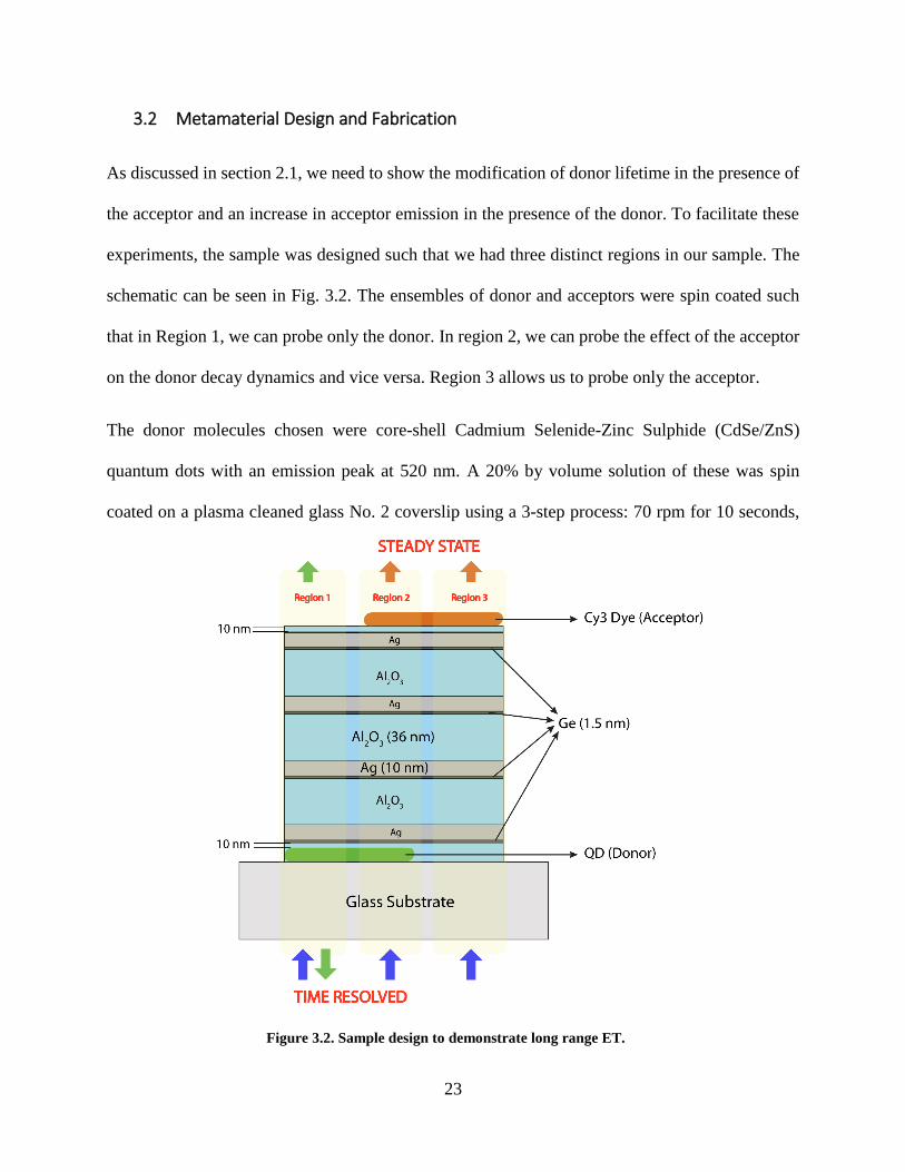
As discussed in section 2.1, we need to show the modification of donor lifetime in the presence of
the acceptor and an increase in acceptor emission in the presence of the donor. To facilitate these
experiments, the sample was designed such that we had three distinct regions in our sample. The
schematic can be seen in Fig. 3.2. The ensembles of donor and acceptors were spin coated such
that in Region 1, we can probe only the donor. In region 2, we can probe the effect of the acceptor
on the donor decay dynamics and vice versa. Region 3 allows us to probe only the acceptor.
The donor molecules chosen were core-shell Cadmium Selenide-Zinc Sulphide (CdSe/ZnS)
quantum dots with an emission peak at 520 nm. A 20% by volume solution of these was spin
coated on a plasma cleaned glass No. 2 coverslip using a 3-step process: 70 rpm for 10 seconds,
Figure 3.2. Sample design to demonstrate long range ET.
24
followed by a short 6 second spin at 150 rpm, finished with a 1300 rpm spin for 30 seconds. The
resultant uniform QD film was 2-3 monolayers thick.
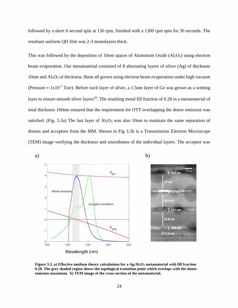
This was followed by the deposition of 10nm spacer of Aluminum Oxide (Al2O3) using electron
beam evaporation. Our metamaterial consisted of 8 alternating layers of silver (Ag) of thickness
10nm and Al2O3 of thickness 36nm all grown using electron beam evaporation under high vacuum
(Pressure ≈ 1x10⁻⁷ Torr). Before each layer of silver, a 1.5nm layer of Ge was grown as a wetting
layer to ensure smooth silver layers26. The resulting metal fill fraction of 0.28 in a metamaterial of
total thickness 160nm ensured that the requirement for OTT overlapping the donor emission was
satisfied. (Fig. 3.3a) The last layer of Al2O3 was also 10nm to maintain the same separation of
donors and acceptors from the MM. Shown in Fig 3.3b is a Transmission Electron Microscope
(TEM) image verifying the thickness and smoothness of the individual layers. The acceptor was
Figure 3.3. a) Effective medium theory calculations for a Ag/Al2O3 metamaterial with fill fraction
0.28. The grey shaded region shows the topological transition point which overlaps with the donor
emission maximum. b) TEM image of the cross-section of the metamaterial.
25
0.67mM of an organic dye, Cyanine 3, spin coated on top using the same recipe as the QDs. The
different regions were formed by dropping the QD and dye at different offsets from the center of
the sample before spin coating.
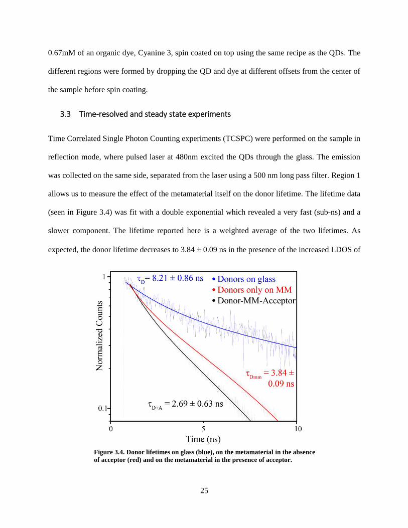
3.3 Time-resolved and steady state experiments
Time Correlated Single Photon Counting experiments (TCSPC) were performed on the sample in
reflection mode, where pulsed laser at 480nm excited the QDs through the glass. The emission
was collected on the same side, separated from the laser using a 500 nm long pass filter. Region 1
allows us to measure the effect of the metamaterial itself on the donor lifetime. The lifetime data
(seen in Figure 3.4) was fit with a double exponential which revealed a very fast (sub-ns) and a
slower component. The lifetime reported here is a weighted average of the two lifetimes. As
expected, the donor lifetime decreases to 3.84 0.09 ns in the presence of the increased LDOS of
Figure 3.4. Donor lifetimes on glass (blue), on the metamaterial in the absence
of acceptor (red) and on the metamaterial in the presence of acceptor.

26
the MM as compared to 8.21 0.86 ns on bare glass. To show ET, donor lifetimes measured in
Region 2 (in the presence of the acceptor) need to be even lower. We measured a lifetime here of
2.69 0.63 ns, which is even less than that measured in Region 1. This ensures that we do indeed
have dipole-dipole interactions between the DA pair.
Time-resolved experiments were also performed with control samples of the DA pairs separated
by 160nm of silver and 160nm of Al2O3 using a geometry similar to the one discussed earlier.
There was no decrease observed in the donor QD lifetimes in the presence of Cyanine 3 acceptor
(red decay curve) on either sample. The data is shown in Figure 3.5. One point to be noted here is
that the donor lifetime in the absence of acceptor is lower than on the metamaterial for both control
cases. The lifetime on Al2O3 is even lower than for silver which is counterintuitive. We could not
determine the cause for this.
To measure the emission increase in the acceptor, experiments were now performed in the
transmission mode, wherein the donor QDs were excited using a 460nm CW diode laser. Steady-
state fluorescence data is collected on the opposite side of the sample. Any emission observed in
Figure 3.5 Donor lifetimes with (red) and without (black) acceptor in control samples where the DA pair is
separated by 160 nm of a) Silver and b) Al2O3

27
Region 3 is because of the laser transmitted through the MM and exciting the dye directly.
However, the thickness of the MM and the fact that excitation of dye is extremely low at 460nm
ensured that there were no emissions in this region. Similarly, any emission from Region 1 is from
the donors directly excited by the laser. These photons will also excite the acceptor and are an
example of photonic transfer of energy. However, energy transfer of this kind does not affect the
decay kinetics of the donor. Dye emission from region 2 has two contributions: photonic transfer
of energy from the donor and ET through resonant dipole-dipole interactions. The former acts as
a background signal which can be accounted for by the measurement in Region 1. Ideally, if we
use a 550 nm filter for the collection, we should be able to filter out a majority of the donor
emission. Unfortunately, the concentration of the QDs used turned out to be quite high and thus,
we had an extremely strong donor emission, enough to completely obscure any signal of the dye
in Region 2. Thus, a 600nm long pass filter was used instead and we observe an increase in
emission in Region 2 as compared to Region 1 (Fig. 3.6a). The difference in the spectrum collected
from these regions should match the emission spectrum of the acceptor and this is verified in Fig
Figure 3.6. a) Steady state emission collected in transmission mode showing increase in acceptor emission.
Also seen is the emission spectrum collected from the donor only which acts as the background. b) Difference
of the two emission spectra (black) in a) superimposed on the acceptor emission spectrum (red).

28
3.6b.
To quantify the direct energy transfer efficiency, we use the formula from equation 2 where τD
(lifetime in absence of acceptor) is the donor lifetime observed in Region 1. We calculate
efficiency of 32% between donors and acceptor separated by 160nm, which is the thickness of the
MM. We also use Equation 2.2 to calculate the energy transfer rate Γ = 0.12 ns-1
There has been another recent report by Newman et. al.27 demonstrating long-range dipole
interaction across a hyperbolic metamaterial of similar thickness. The authors note that a single
donor dipole can interact with many physically separated acceptor dipoles all along the other
surface. If we consider this assertion, our sample geometry with the separate regions is not as
elegant as hoped. However, this does not invalidate our results. The interaction with multiple
acceptor dipoles would imply that donor lifetime measurements in Region 1 would already
encounter the effect of some acceptor molecules. Thus the “true” lifetime in the absence of
acceptor would be even higher. It follows that our measurement represents the lowest possible rate
of energy transfer through dipole interactions. Despite this limitation, we still show ET through
dipole interactions across a DA separation of 160nm.
All the examples discussed so far from literature and our own experiment are examples of the
approach of modifying the density of states in the system. An alternative approach is to use strong
coupling to achieve the similar increase in the efficiency of long-range ET. This was demonstrated
in microcavity systems where the donor acceptor pairs are strongly coupled to the cavity mode.
28,29 Similar effects have also been demonstrated by coupling to plasmonic based systems.30,31 It is
possible that the observed increase in ET efficiency might be related to delocalization of the
exciton wavefunction occurring due to strong coupling in such systems. If true, this would be
29
similar to photosynthetic light harvesting, where it is also suspected that quantum coherence plays
a major role.32,33 Recently, enhanced ET was shown for spatially separated DA systems in a
strongly coupled state in microcavity.34 Further theoretical investigations isolate the role of
strongly coupled donors and strongly coupled acceptors in this process.35,36 This was investigated
for the case of strong coupling with surface plasmons. While we do not explore the possibility of
using this principle in this thesis, it is important to note the role played by the formation of the new
eigenstates brought about by strong coupling lending the hybrid characters to the exciton. This will
have important consequences for our work in Chapter 4.
In summary, we designed a donor-MM-acceptor system such that the OTT of the MM occurs at
the maximum spectral overlap of the donor emission and acceptor excitation. The significant
increase in available LDOS allowed us to verify energy transfer at 32% efficiency directly through
dipole-dipole interactions across 160nm. A notable point is that the scheme can be customized for
any donor-acceptor pair by simply adjusting the metal fill fraction in the metamaterial and thus,
tuning the OTT. While it seems unlikely that the geometry used here will be useful in actual
experiments, it serves as a proof-of-principle and it is hoped that more favorable geometries, for
example in metasurfaces, could be used for real-world applications in pushing the boundaries of
RET.
30
4.1 Introduction
In Chapter 3, we summarized literature hinting that the hybrid nature imparted to an exciton could
be used to enhance the efficiency of RET. This is an important example of how strong light-matter
interaction can be used to affect the dynamics of the excited energy states in molecules. In this
chapter, we will use another effect of strong coupling – the creation of new eigen states for the
coupled system – and demonstrate that this can also be used to control another aspect of excited
state dynamics, that of chemical transformations.
The role of strong coupling in controlling chemical reactions was first proposed by the group of
Thomas Ebbesen. They first reported in 201237, the suppression of the photooxidation process of
an organic molecule spyropyran to merocyanine, using strong coupling of a cavity to the resonance
associated with the merocyanine absorption. Theoretical studies by Galego et. al38 supported the
phenomenon. Alternate approaches were suggested by Herrera and Spano39, where they used
strong coupling to provide a model for decoupling of collective electronic and nuclear degrees of
freedom in disordered organic molecules and enhance the rate of electron transport reactions.
Shalabney et. al. suggested strong coupling of vibrational energy levels in molecules to cavity
fields as a way of modifying bond strengths and affect chemical reactions40. Following up on these
examples, we demonstrate here that ultra-strong coupling can be used to affect the Excited State
4 Modifying rate of Excited State Intramolecular Proton Transport using
Cavity Ultra-Strong Coupling
31
Intramolecular Proton Transport (ESIPT) process in an organic molecule and suppress its
photoluminescence.
ESIPT is a process involving the transfer of a proton through a pre-existing hydrogen bonding
configuration in organic molecules. As it is a reaction involving the transfer of a proton,
understanding the dynamics is important to be able to control many chemical and biological
reactions. This proton transfer is an extremely fast process and has been studied in various
molecules to uncover its dynamics and kinetics41–44. They report that the process is extremely fast,
and the dynamics are practically barrierless in many cases45. Molecules which exhibit ESIPT are
generally characterized by a much larger Stoke shift compared to more commonly used
fluorophores. These studies have led to applications as molecular probes46, materials for lasing47
and white light generation48, organic LED’s49,50 and the like. Controlling the process using strong
coupling would be a new approach where we attempt to control the energy levels instead of just
the environment around the reaction sites as done in previous studies.
4.2 Sample fabrication and demonstration of strong coupling
The molecular system that we use is 3-(dimethylamino)-1-(2-hydroxy-4-methoxyphenyl)-2-
propen-1-one (HMPP). It exists in enol form in the ground state. Upon UV excitation, ESIPT leads
to the formation of the keto tautomer and the molecule relaxes to the ground state of the keto form
which results in highly Stoke shifted emission. It has a high quantum yield in the solid state and
consequently, its emission intensity is highly increased in the PMMA matrix compared to its
solution state because of aggregation induced enhanced emission. Figure 4.1a) shows a schematic
of the tautomer forms. b) shows the absorption maximum at ~355nm and the Stoke shifted
emission from the keto form at a maximum of ~ 500 nm. In Figure 4.1 c) we have shown a highly
simplified cartoon for the ESIPT process, neglecting many details for the sake of simplicity. If

32
strong coupling can be achieved with the excited enol form and the new eigenstates created (shown
by the dotted levels), it might be possible to alter the dynamics of the process and perhaps slow
down the transport process by decreasing the energy difference between the tautomeric forms and
thus, induce a small barrier in the dynamics.
Our sample cavities were designed to be resonant at 355nm. They consisted of 20nm of metallic
silver grown on clean glass micro slips in an E-beam evaporator, followed by a spacer layer of
5nm Al2O3 to separate the HMPP from the silver. The cavity layers were formed by differing
concentration of HMPP in 495 PMMA A2 (Michrochem). The spin coating recipe is varied to get
layer thicknesses as uniform as possible across different samples. Addition of the HMPP into the
PMMA A2 solution makes it considerably more viscous and this viscosity increase depends on the
concentration of HMPP added. (Note: Concentrations will be denoted by the unusual units of
mg/0.5mL. They happened to be chosen for experimental convenience.) Therefore, before spin
coating, the solutions were diluted with appropriately calculated volumes of the solvent Anisole.
The hard baking step for PMMA is also avoided. Baking above 100ºC deactivates the HMPP and
Figure 4.1 a) Tautomeric forms of HMPP. b) Absorption (black) and emission (red) spectra for
HMPP in a PMMA matrix. c) Cartoon showing the ESIPT process and the attempted change.

33
renders it useless for the experiment. Finally, another 5nm of Al2O3 and 20nm of silver were added
to complete the metallic cavity.
To determine the extent of coupling, we must rely on transmission measurements instead of
reflection measurements as the UV range is not suitable for available detectors and light sources.
The angle-resolved transmission measurements were performed using a Horiba Fluoromax
spectrometer. The data is shown in Figure 4.2 for three different concentrations are shown. The
0.02mg/0.5mL HMPP sample shows only one peak following the original cavity distribution and
is thus, a clear example of a weakly coupled cavity. The 1.5mg sample, on the other hand, showed
prominent double peaks in its transmission spectrum. The dispersion of these peaks, especially the
high energy peak, is quite small, but nonetheless, is present. These are signatures of strong
coupling and can be termed as the upper and lower polariton branches. Moving to a higher
concentration, at 8mg, the Rabi split between the polariton branches becomes even larger. Figure
4.3 shows the observed transmission spectra peaks as a function of concentration and angle. We
clearly see a jump in behavior between the 0.02mg and 1.5mg sample where the transition from
weak to strong coupling occurs.
Figure 4.2 Transmission measurements for HMPP in a cavity showing examples of a) weak coupling, b) Strong
coupling and c) Ultra strong coupling.
34
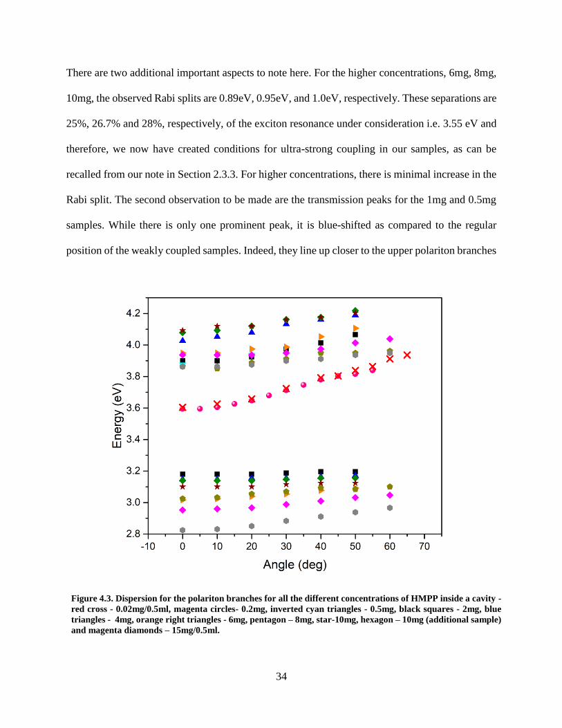
There are two additional important aspects to note here. For the higher concentrations, 6mg, 8mg,
10mg, the observed Rabi splits are 0.89eV, 0.95eV, and 1.0eV, respectively. These separations are
25%, 26.7% and 28%, respectively, of the exciton resonance under consideration i.e. 3.55 eV and
therefore, we now have created conditions for ultra-strong coupling in our samples, as can be
recalled from our note in Section 2.3.3. For higher concentrations, there is minimal increase in the
Rabi split. The second observation to be made are the transmission peaks for the 1mg and 0.5mg
samples. While there is only one prominent peak, it is blue-shifted as compared to the regular
position of the weakly coupled samples. Indeed, they line up closer to the upper polariton branches
Figure 4.3. Dispersion for the polariton branches for all the different concentrations of HMPP inside a cavity -
red cross - 0.02mg/0.5ml, magenta circles- 0.2mg, inverted cyan triangles - 0.5mg, black squares - 2mg, blue
triangles - 4mg, orange right triangles - 6mg, pentagon – 8mg, star-10mg, hexagon – 10mg (additional sample)
and magenta diamonds – 15mg/0.5ml.
35
of the strongly coupled samples. We also see a very weak maximum close to the lower polariton
branch. We interpret this zone as sitting at the borderline between weak and strong coupling.
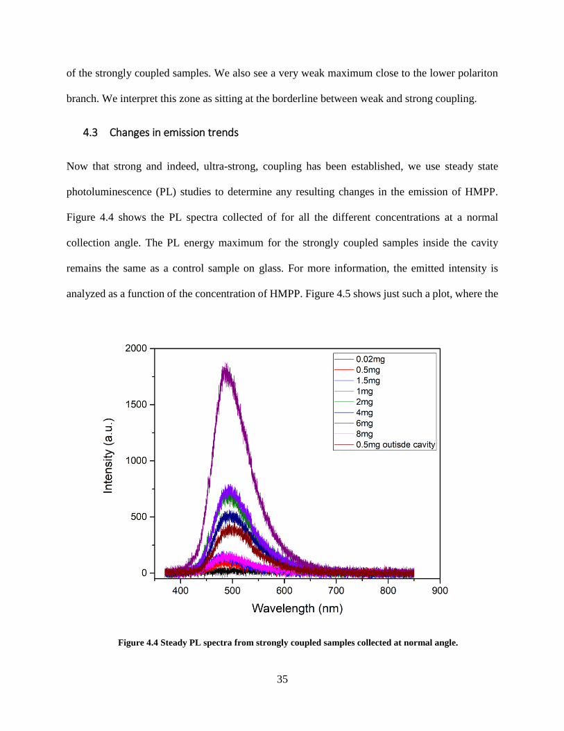
4.3 Changes in emission trends
Now that strong and indeed, ultra-strong, coupling has been established, we use steady state
photoluminescence (PL) studies to determine any resulting changes in the emission of HMPP.
Figure 4.4 shows the PL spectra collected of for all the different concentrations at a normal
collection angle. The PL energy maximum for the strongly coupled samples inside the cavity
remains the same as a control sample on glass. For more information, the emitted intensity is
analyzed as a function of the concentration of HMPP. Figure 4.5 shows just such a plot, where the
Figure 4.4 Steady PL spectra from strongly coupled samples collected at normal angle.

36
red circles show the data for the control samples and the black circles represent the strongly
coupled samples. We see that the collected emission is much weaker as compared to the control
samples, but this, by itself, is not necessarily significant. We need to take into account several
different correction factors to make an accurate comparison of the two different sets of data:
i) The electric field experienced by the molecules inside the cavity is not the same as that
for the control sample. There have been no corrections to account for any field
confinement or enhancement because of the cavity.
ii) The emission observed at the detector will also require a corrective factor as a
significant number of emitted photons might be trapped within the cavity as well.
iii) Losses/enhancements occurring because of the proximity of the aluminum layers.
Figure 4.5 Comparison of emission from HMPP inside the cavity (black squares) vs control sample
without cavity (red circles)
37
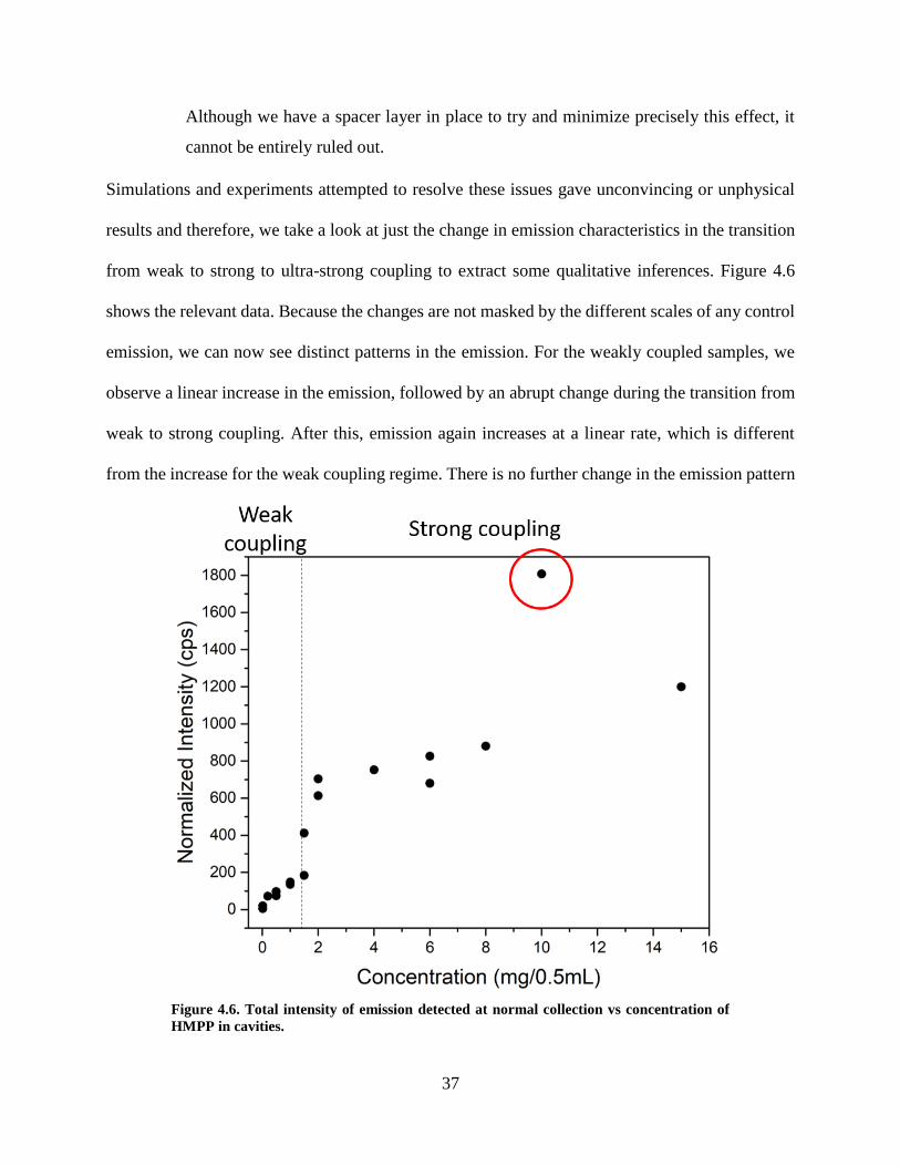
Although we have a spacer layer in place to try and minimize precisely this effect, it
cannot be entirely ruled out.
Simulations and experiments attempted to resolve these issues gave unconvincing or unphysical
results and therefore, we take a look at just the change in emission characteristics in the transition
from weak to strong to ultra-strong coupling to extract some qualitative inferences. Figure 4.6
shows the relevant data. Because the changes are not masked by the different scales of any control
emission, we can now see distinct patterns in the emission. For the weakly coupled samples, we
observe a linear increase in the emission, followed by an abrupt change during the transition from
weak to strong coupling. After this, emission again increases at a linear rate, which is different
from the increase for the weak coupling regime. There is no further change in the emission pattern
Figure 4.6. Total intensity of emission detected at normal collection vs concentration of
HMPP in cavities.
38
for higher concentrations. We do note the anomalous data for the 10mg samples, where the
emission is far stronger than any other concentrations. However, in the absence of any pattern, it
may be ascribed to experimental error, perhaps in the concentration of the sample or occurrence
of defects in the cavity. Time-resolved PL could not be obtained because of the absence of strong
pulsed excitation sources at the required wavelength of 350nm. In the absence of such data, no
concrete conclusions can be drawn, however, simulations by collaborators point towards
reasonable inferences.
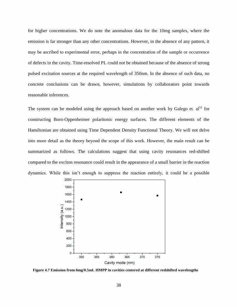
The system can be modeled using the approach based on another work by Galego et. al51 for
constructing Born-Oppenheimer polaritonic energy surfaces. The different elements of the
Hamiltonian are obtained using Time Dependent Density Functional Theory. We will not delve
into more detail as the theory beyond the scope of this work. However, the main result can be
summarized as follows. The calculations suggest that using cavity resonances red-shifted
compared to the exciton resonance could result in the appearance of a small barrier in the reaction
dynamics. While this isn’t enough to suppress the reaction entirely, it could be a possible
Figure 4.7 Emission from 6mg/0.5mL HMPP in cavities centered at different redshifted wavelengths
39
explanation for the change in emission patterns. Unfortunately, cavity samples with a resonance
at 363nm and 375nm failed to show any difference in emission when compared to the cavity at
350nm. The data is shown in Figure 4.7. It is difficult to perform clean experiments for even more
red shifted cavities as higher order modes start overlapping with our original exciton.
In summary, we have demonstrated ultra-strong coupling of a molecule, HMPP, to a metallic
cavity with the objective of modifying the ESIPT process in HMPP. Concentration-dependent
studies show that the Rabi splitting almost gets saturated at higher concentrations. While emission
patterns do get modified under strong coupling, the reasons are not well understood. Further
experiments could be warranted with a different system that is more convenient for probing the
dynamics using time-resolved spectroscopy. The field of strong coupling based chemical reactions
is still very nascent and finding the correct system for such experiments is critical.
40
5.1 Introduction
In Chapters 3 and 4, we have seen that the phenomenon of strong light-matter interaction between
different photonic structures and excitons can and has been used in a wide range of research
directions. To that end, within the optical regime, the demonstration of strong coupling has been
seen in a variety of systems, starting with multiple atoms in a cavity in 198952. This has been
followed by demonstrations with single atoms53 and the first demonstration of strong coupling
with a solid-state system in optical microcavity54. A good review of immediate further
developments may be found in the paper by Skolnick et.al55. The earlier demonstrations were all
at cryogenic temperatures with the first room temperature example of strong coupling coming in
199456,57. All these demonstrations were with inorganic materials and the observed normal mode
or Rabi splitting were of the order of few meV.
The first example of strong coupling with organic materials was shown by Lidzey et. al. in 199858.
This and subsequent demonstrations could be achieved at room temperature with Rabi splitting of
the order of hundreds of meV. This is because of the tightly bound excitons of organic materials
have a high oscillator strength which allowed for easier achievement of strong coupling. In recent
years strong coupling with organic molecules have been used to replicate most of the interesting
5 Modification of photoluminescence spectra using strong coupling of
vibronic transitions in organic molecules with surface plasmons
41
results achieved with inorganic materials and semiconductors, such as Bose Einstein-like polariton
condensation59, and superfluidity60 at room temperature.
There have also been several reports of strong coupling between other photonic structures like
surface plasmons, photonic crystals, micro-ring resonators and optomechanical cavities with other
material resonances like phonons61. However, there have been very few reports of strong coupling
with vibronic transitions. These are resonances arising from simultaneous changes in the electronic
and vibrational energy levels. These transitions are governed by the Franck Condon principles and
are only allowed if there is significant wavefunction overlap between the vibrational levels in the
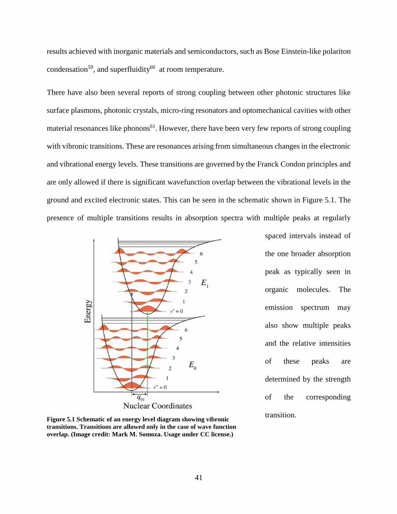
ground and excited electronic states. This can be seen in the schematic shown in Figure 5.1. The
presence of multiple transitions results in absorption spectra with multiple peaks at regularly
spaced intervals instead of
the one broader absorption
peak as typically seen in
organic molecules. The
emission spectrum may
also show multiple peaks
and the relative intensities
of these peaks are
determined by the strength
of the corresponding
transition.
Figure 5.1 Schematic of an energy level diagram showing vibronic
transitions. Transitions are allowed only in the case of wave function
overlap. (Image credit: Mark M. Somoza. Usage under CC license.)
42
The only reports of strong coupling with vibronic transitions are with microcavities56,62,63. In this
chapter, we will discuss our work in strong coupling between vibronic transitions in an organic
molecule with surface plasmon polaritons (SPP) on silver and the interesting modification in the
photoluminescence from the molecule.
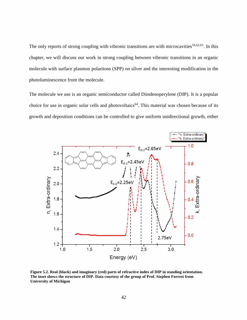
The molecule we use is an organic semiconductor called Diindenoperylene (DIP). It is a popular
choice for use in organic solar cells and photovoltaics64. This material was chosen because of its
growth and deposition conditions can be controlled to give uniform unidirectional growth, either
Figure 5.2. Real (black) and imaginary (red) parts of refractive index of DIP in standing orientation.
The inset shows the structure of DIP. Data courtesy of the group of Prof. Stephen Forrest from
University of Michigan

43
in a standing orientation or flat-lying orientation. In this project, up-standing orientation was
favored for better coupling to the surface plasmon mode. The absorption spectrum in Fig. 5.2
shows E0-0, E0-1, E0-2 transitions occurring separated by 200 meV. There is a fourth peak at 2.75
eV that does not follow the pattern but is probably a result of Davidoff splitting arising out of
interaction with the crystal structure.
5.2 Experiment Design and Reflectivity
Our sample was a 50nm film of Ag evaporated on a 2nm Ge Wetting layer on a glass substrate.
There was also a 3nm Al2O3 spacer layer. The Al2O3 also prevents oxidation of the silver layer.
30nm DIP was thermally evaporated on top. Atomic Force Microscope measurements verify that
the DIP molecules tend to be vertically aligned. The same thickness of DIP was also evaporated
on Silicon substrate for control measurements. Angle-resolved reflectivity measurements were
Figure 5.3 Schematic of Angle resolved reflection experiment for DIP on silver.
44
performed in the Kretschmann configuration. Figure 5.3 shows a schematic for the configuration
where TM polarized white light is incident on the sample on the substrate side through a prism.
For a bare silver sample, we see one just the one SPP mode (refer to Section 2.4). The sample with
the DIP, on the other hand, shows multiple dips at every angle. Figure 6.4 shows the reflectivity
as a function of incident energy of light for angles ranging from 46° to 69°. Also seen is the
extinction data for the bare DIP molecule. The peaks correspond to the energy levels of the
vibronic transitions. There are multiple avoided crossings seen in the reflectivity data which align
perfectly with the vibronic transition energies, which is a clear case for strong coupling. The color
plot in Figure 5.5a shows the reflectivity simulated for the same sample using transfer matrix
approach. The experimental data points collected are plotted as individual points on top and there
is good agreement between the two. To calculate the Rabi splittings, we need to plot the same data
in the Energy-momentum plane (reference). The results are shown in Fig 5.5b. The experimentally
observed Rabi splittings are 94meV for the E0-0, 131meV for E0-1 and 170 meV for E0-2 transitions.
We also use the coupled oscillator model described earlier to calculate the Hopfield coefficients
seen in Figure 5.6.

45
Figure 5.4 Angle resolved reflectivity data from 46º to 69º from 30nm DIP on
Silver. The avoided crossings line up perfectly with the vibronic transition
peaks for DIP.

46
We also use the coupled oscillator model described earlier in section 2. to calculate the Hopfield
coefficients seen in Fig 5.6. The calculated coefficients are along expected lines, with the lowest
branch containing the most contribution from the SPP at low angles and the E0-0 vibronic at high
angles. The contribution of the SPP is decreased for the middle branches and reappears again at
large angles for the uppermost branch.
Figure 5.5 a) Dispersion data for the strongly coupled DIP sample overlaid on simulation results. Horizontal white dashes
are the peaks from absorption spectrum. White dashed curve represents dispersion for a bare silver film modified to take
into account 30nm of dielectric spacer with the same real part of refractive index as DIP. b) Same dispersion data now
plotted in E vs kx. The red dashed lines are the light lines for air and prism. The green curve represents the same
modified dispersion of a bare silver film as in a).

47
5.3 Photoluminescence modification
In most reports of emission studies from strong coupling with surface plasmon polaritons, emission
studies are performed by exciting the emitters directly and collecting leakage radiation through the
prism side into the far field and guiding it through a spectrometer. This situation is analogous to
the polariton emission experiments in cavities where the emission always carries a signature of the
cavity itself, viz. in the form of the dispersion which follows that observed for the polariton
branches in reflection experiments. (We will revisit this point during the discussion of the emission
data.) There are only a very few prominent examples in which the emission is collected on the
Figure 5.6 Calculated Hopfield coefficients for the different polariton branches.
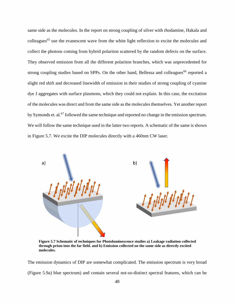
48
same side as the molecules. In the report on strong coupling of silver with rhodamine, Hakala and
colleagues65 use the evanescent wave from the white light reflection to excite the molecules and
collect the photons coming from hybrid polariton scattered by the random defects on the surface.
They observed emission from all the different polariton branches, which was unprecedented for
strong coupling studies based on SPPs. On the other hand, Bellessa and colleagues66 reported a
slight red shift and decreased linewidth of emission in their studies of strong coupling of cyanine
dye J aggregates with surface plasmons, which they could not explain. In this case, the excitation
of the molecules was direct and from the same side as the molecules themselves. Yet another report
by Symonds et. al.67 followed the same technique and reported no change in the emission spectrum.
We will follow the same technique used in the latter two reports. A schematic of the same is shown
in Figure 5.7. We excite the DIP molecules directly with a 460nm CW laser.
The emission dynamics of DIP are somewhat complicated. The emission spectrum is very broad
(Figure 5.9a) blue spectrum) and contain several not-so-distinct spectral features, which can be
Figure 5.7 Schematic of techniques for Photoluminescence studies a) Leakage radiation collected
through prism into the far field. and b) Emission collected on the same side as directly excited
molecules.
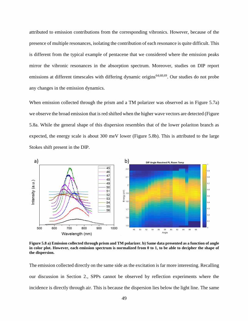
49
attributed to emission contributions from the corresponding vibronics. However, because of the
presence of multiple resonances, isolating the contribution of each resonance is quite difficult. This
is different from the typical example of pentacene that we considered where the emission peaks
mirror the vibronic resonances in the absorption spectrum. Moreover, studies on DIP report
emissions at different timescales with differing dynamic origins64,68,69. Our studies do not probe
any changes in the emission dynamics.
When emission collected through the prism and a TM polarizer was observed as in Figure 5.7a)
we observe the broad emission that is red shifted when the higher wave vectors are detected (Figure
5.8a. While the general shape of this dispersion resembles that of the lower polariton branch as
expected, the energy scale is about 300 meV lower (Figure 5.8b). This is attributed to the large
Stokes shift present in the DIP.
The emission collected directly on the same side as the excitation is far more interesting. Recalling
our discussion in Section 2., SPPs cannot be observed by reflection experiments where the
incidence is directly through air. This is because the dispersion lies below the light line. The same
Figure 5.8 a) Emission collected through prism and TM polarizer. b) Same data presented as a function of angle
in color plot. However, each emission spectrum is normalized from 0 to 1, to be able to decipher the shape of
the dispersion.

50
principle follows in the time-reversed process. An SPP cannot scatter as a photon directly into air
as the momentum matching conditions are forbidden. Therefore, we now have a rather interesting
possibility of observing emission from molecules which have been affected by strong coupling
with a photonic mode, without seeing any effect of the photonic mode dispersion itself. This is
not possible in any other strongly coupled systems as cavities, plasmonic lattices and photonic
crystals etc. can all be coupled to light from free space and therefore polariton emission always
follows the dispersion of the strongly coupled system. To re-emphasize, emission observed using
this detection technique contains contributions from uncoupled molecules (which can be easily
checked using control samples on a different dielectric substrate) and contributions from molecules
strongly coupled to the SPP. It is only the observation of SPP that requires excitation through a
prism. The system itself remains in a strongly coupled state through coupling via vacuum
fluctuations irrespective of the excitation.
With this discussion in mind, we now report the emission collected using technique b in Figure
5.9a). The emission from the strongly coupled DIP on silver is seen in red. For comparison, we
have also shown, the emission spectrum from a control film of DIP grown at the same time on a
Silicon substrate. Both spectra have been normalized from 0 to 1 to see any difference. We can
clearly see a change as the strongly coupled sample seems to have a more uniform contribution
from all the vibronic resonances. However, the very broad emissions make it difficult to draw any
further conclusions and therefore, the same experiment was repeated at 77K. Due to the decrease
in inhomogeneous broadening at cryogenic temperatures, we see a much clearer picture of the
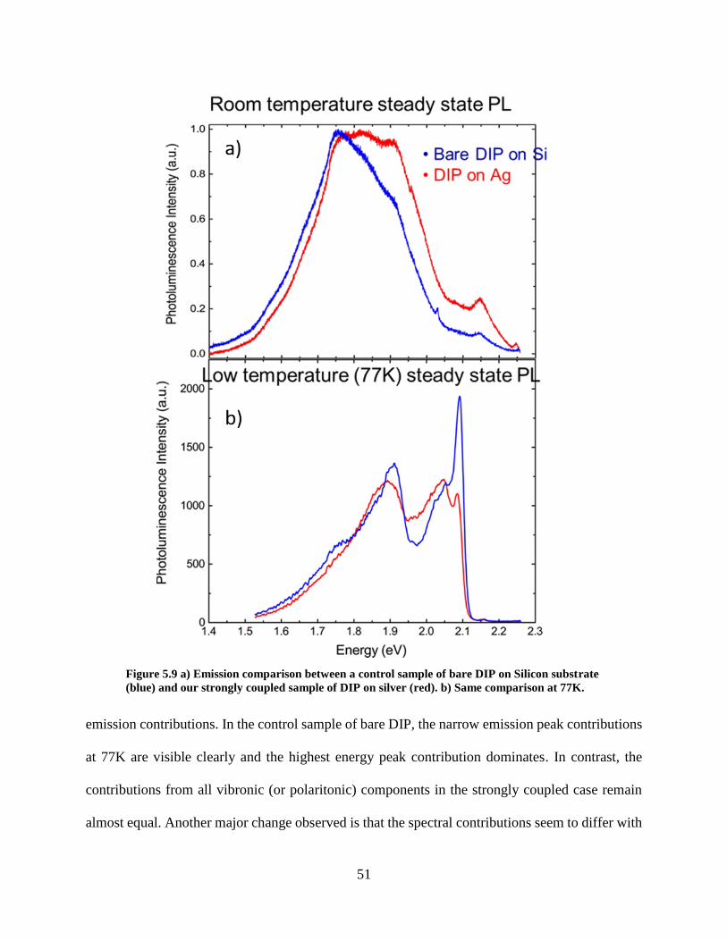
51
emission contributions. In the control sample of bare DIP, the narrow emission peak contributions
at 77K are visible clearly and the highest energy peak contribution dominates. In contrast, the
contributions from all vibronic (or polaritonic) components in the strongly coupled case remain
almost equal. Another major change observed is that the spectral contributions seem to differ with
Figure 5.9 a) Emission comparison between a control sample of bare DIP on Silicon substrate
(blue) and our strongly coupled sample of DIP on silver (red). b) Same comparison at 77K.

52
temperature as well. (high energy peak at low temperature vs low energy peak at room temperature
in bare DIP).
Temperature-dependent PL studies were performed to verify the change in contribution due to
temperature. We only show the results from 90 K to 160 K for the sake of clarity as this is the
temperature range where the maximum change is observed. In Figure 5.10a) we observe the
systematic change in the contribution of the peaks from higher energy to lower energy as we start
increasing temperature. At 70K, the high energy peak at 2.1 eV is the most dominant while the
lower energy peaks cannot be seen on the same scale. The spectrum remains very similar when
the temperature is lowered further. As the temperature starts increasing, first the peak ~2.1 eV and
then the peak at ~2.05eV starts rapidly decreasing in contribution till it almost disappears
completely. The other peaks are slower to degrade. The main change beyond 160K is that the
remaining peak ~1.9eV also decays which leaves the lower energy peaks closer to ~1.7eV as the
dominant ones.
In contrast, the strongly coupled DIP has very equal contributions even at 70K. With increase in
temperature, the higher energy peaks are much more persistent as the 2.05 eV peak only starts to
decrease around 160K. By room temperature, 2.05eV and 2.1eV are the only peaks to decay
significantly while all others remain prominent and contribute equally.

53
Figure 5.10 Temperature dependent photoluminescence spectra from a) control sample
and b) strongly coupled sample.
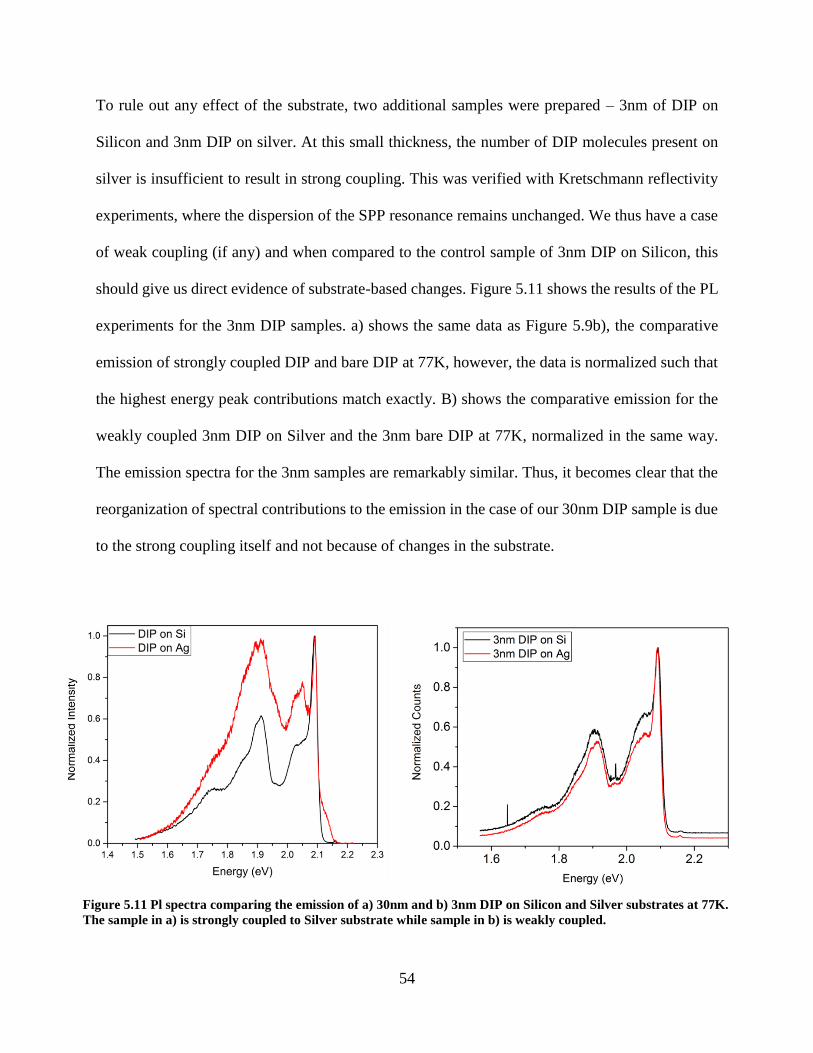
54
To rule out any effect of the substrate, two additional samples were prepared – 3nm of DIP on
Silicon and 3nm DIP on silver. At this small thickness, the number of DIP molecules present on
silver is insufficient to result in strong coupling. This was verified with Kretschmann reflectivity
experiments, where the dispersion of the SPP resonance remains unchanged. We thus have a case
of weak coupling (if any) and when compared to the control sample of 3nm DIP on Silicon, this
should give us direct evidence of substrate-based changes. Figure 5.11 shows the results of the PL
experiments for the 3nm DIP samples. a) shows the same data as Figure 5.9b), the comparative
emission of strongly coupled DIP and bare DIP at 77K, however, the data is normalized such that
the highest energy peak contributions match exactly. B) shows the comparative emission for the
weakly coupled 3nm DIP on Silver and the 3nm bare DIP at 77K, normalized in the same way.
The emission spectra for the 3nm samples are remarkably similar. Thus, it becomes clear that the
reorganization of spectral contributions to the emission in the case of our 30nm DIP sample is due
to the strong coupling itself and not because of changes in the substrate.
Figure 5.11 Pl spectra comparing the emission of a) 30nm and b) 3nm DIP on Silicon and Silver substrates at 77K.
The sample in a) is strongly coupled to Silver substrate while sample in b) is weakly coupled.

55
In summary, we have shown in this chapter, an example of strong coupling of vibronic transitions
in an organic molecule, DIP to the SPP on a silver film. We discuss the advantage offered by the
technique we use for the PL studies. The collection of emission on the same side as direct excitation
might give us a clue to a fundamental question: are there any changes to the basic properties of
any material as a result of hybridization with a photonic component using strong coupling? In this
case, the strong coupling results in a significant spectral weight redistribution in the contribution
to emission from different vibronic resonances. However, it is worth noting that previous reports
using the same technique talk about very little or no changes in the emission. One possible reason
for this difference could be that those reports discuss strong coupling with one or two excitons as
opposed to our study in we use multiple vibronic transitions. If that is indeed the case, it hints that
much more remains to be understood about the emission processes in such systems. If similar
experiments can be performed with organic materials in which we have a much better
understanding of the emission dynamics and with cleaner emission spectra, like that in pentacene,
it is possible that we could have a clearer picture about the physics of vibronic transitions and the
phenomenon of strong coupling itself.
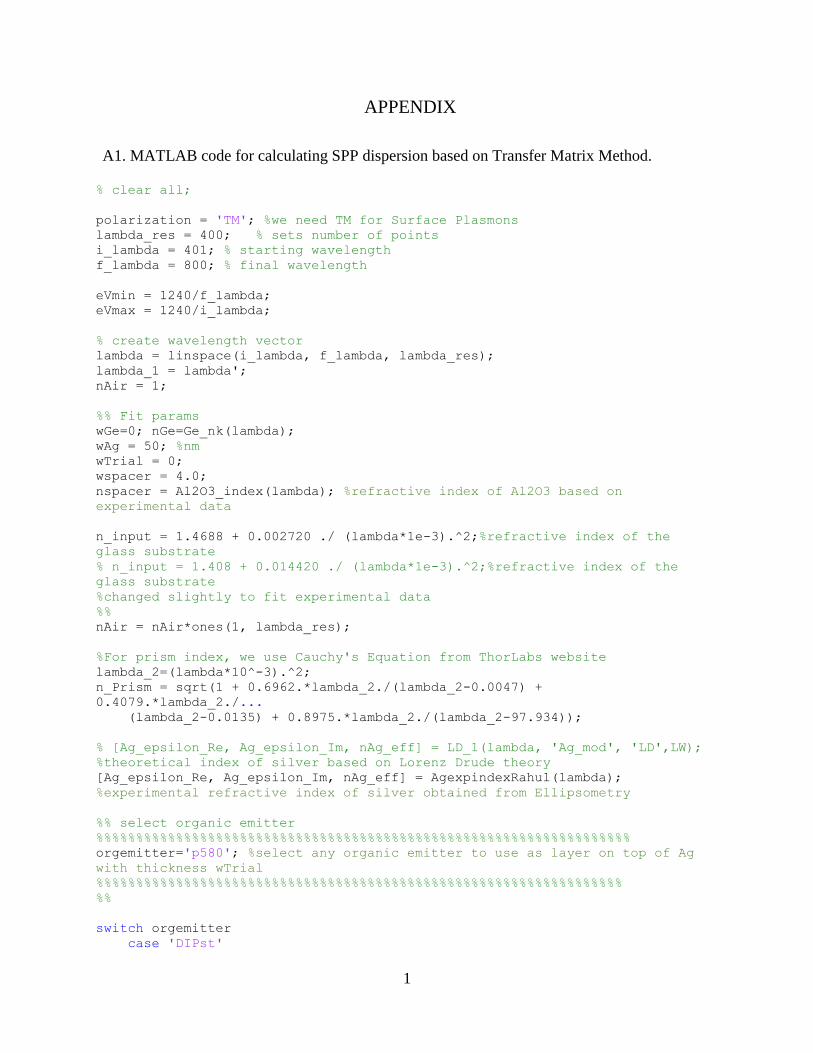
1
APPENDIX
A1. MATLAB code for calculating SPP dispersion based on Transfer Matrix Method.
% clear all;
polarization = 'TM'; %we need TM for Surface Plasmons
lambda_res = 400; % sets number of points
i_lambda = 401; % starting wavelength
f_lambda = 800; % final wavelength
eVmin = 1240/f_lambda;
eVmax = 1240/i_lambda;
% create wavelength vector
lambda = linspace(i_lambda, f_lambda, lambda_res);
lambda_1 = lambda';
nAir = 1;
%% Fit params
wGe=0; nGe=Ge_nk(lambda);
wAg = 50; %nm
wTrial = 0;
wspacer = 4.0;
nspacer = Al2O3_index(lambda); %refractive index of Al2O3 based on
experimental data
n_input = 1.4688 + 0.002720 ./ (lambda*1e-3).^2;%refractive index of the
glass substrate
% n_input = 1.408 + 0.014420 ./ (lambda*1e-3).^2;%refractive index of the
glass substrate
%changed slightly to fit experimental data
%%
nAir = nAir*ones(1, lambda_res);
%For prism index, we use Cauchy's Equation from ThorLabs website
lambda_2=(lambda*10^-3).^2;
n_Prism = sqrt(1 + 0.6962.*lambda_2./(lambda_2-0.0047) +
0.4079.*lambda_2./...
(lambda_2-0.0135) + 0.8975.*lambda_2./(lambda_2-97.934));
% [Ag_epsilon_Re, Ag_epsilon_Im, nAg_eff] = LD_1(lambda, 'Ag_mod', 'LD',LW);
%theoretical index of silver based on Lorenz Drude theory
[Ag_epsilon_Re, Ag_epsilon_Im, nAg_eff] = AgexpindexRahul(lambda);
%experimental refractive index of silver obtained from Ellipsometry
%% select organic emitter
%%%%%%%%%%%%%%%%%%%%%%%%%%%%%%%%%%%%%%%%%%%%%%%%%%%%%%%%%%%%%%%%%%%
orgemitter='p580'; %select any organic emitter to use as layer on top of Ag
with thickness wTrial
%%%%%%%%%%%%%%%%%%%%%%%%%%%%%%%%%%%%%%%%%%%%%%%%%%%%%%%%%%%%%%%%%%
%%
switch orgemitter
case 'DIPst'
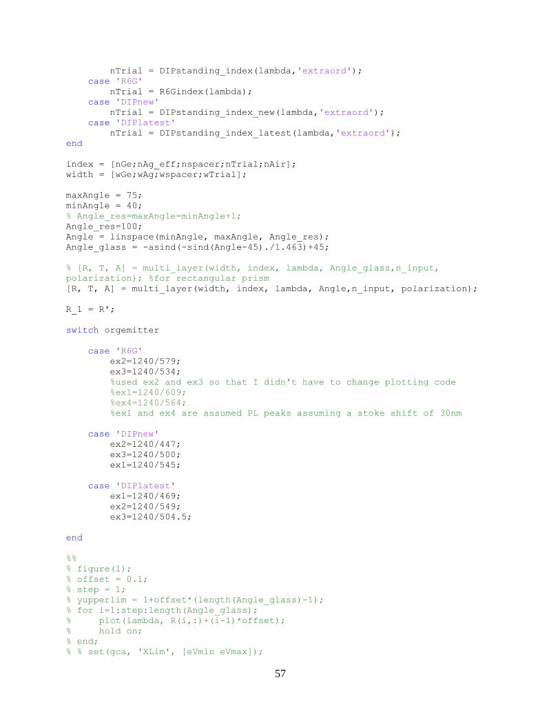
57
nTrial = DIPstanding_index(lambda,'extraord');
case 'R6G'
nTrial = R6Gindex(lambda);
case 'DIPnew'
nTrial = DIPstanding_index_new(lambda,'extraord');
case 'DIPlatest'
nTrial = DIPstanding_index_latest(lambda,'extraord');
end
index = [nGe;nAg_eff;nspacer;nTrial;nAir];
width = [wGe;wAg;wspacer;wTrial];
maxAngle = 75;
minAngle = 40;
% Angle_res=maxAngle-minAngle+1;
Angle_res=100;
Angle = linspace(minAngle, maxAngle, Angle_res);
Angle_glass = -asind(-sind(Angle-45)./1.463)+45;
% [R, T, A] = multi_layer(width, index, lambda, Angle_glass,n_input,
polarization); %for rectangular prism
[R, T, A] = multi_layer(width, index, lambda, Angle,n_input, polarization);
R_1 = R';
switch orgemitter
case 'R6G'
ex2=1240/579;
ex3=1240/534;
%used ex2 and ex3 so that I didn't have to change plotting code
%ex1=1240/609;
%ex4=1240/564;
%ex1 and ex4 are assumed PL peaks assuming a stoke shift of 30nm
case 'DIPnew'
ex2=1240/447;
ex3=1240/500;
ex1=1240/545;
case 'DIPlatest'
ex1=1240/469;
ex2=1240/549;
ex3=1240/504.5;
end
%%
% figure(1);
% offset = 0.1;
% step = 1;
% yupperlim = 1+offset*(length(Angle_glass)-1);
% for i=1:step:length(Angle_glass);
% plot(lambda, R(i,:)+(i-1)*offset);
% hold on;
% end;
% % set(gca, 'XLim', [eVmin eVmax]);
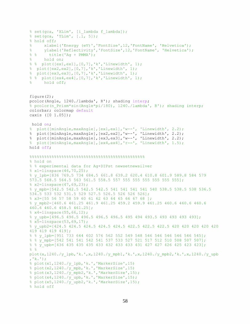
58
% set(gca, 'XLim', [i_lambda f_lambda]);
% set(gca, 'YLim', [.1, 5]);
% hold off;
% xlabel('Energy (eV)','FontSize',12,'FontName', 'Helvetica');
% ylabel('Reflectivity','FontSize',12,'FontName', 'Helvetica');
% % title('Ag + PMMA');
% hold on;
% % plot([ex1,ex1],[0,7],'k','Linewidth', 1);
% plot([ex2,ex2],[0,7],'k','Linewidth', 1);
% plot([ex3,ex3],[0,7],'k','Linewidth', 1);
% % plot([ex4,ex4],[0,7],'k','Linewidth', 1);
% hold off;
figure(2);
pcolor(Angle, 1240./lambda', R'); shading interp;
% pcolor(n_Prism*sin(Angle*pi/180), 1240./lambda', R'); shading interp;
colorbar; colormap default
caxis ([0 1.05]);
hold on;
% plot([minAngle,maxAngle],[ex1,ex1],'w--', 'Linewidth', 2.2);
% plot([minAngle,maxAngle],[ex2,ex2],'w--', 'Linewidth', 2.2);
% plot([minAngle,maxAngle],[ex3,ex3],'w--', 'Linewidth', 2.2);
% plot([minAngle,maxAngle],[ex4,ex4],'r--', 'Linewidth', 1.5);
hold off;
%%%%%%%%%%%%%%%%%%%%%%%%%%%%%%%%%%%%%%%%%%%%%%%
% hold on
% % experimental data for Ag+DIPst newsetnewsilver
% x1=linspace(46,70,25);
% y_lpb=[836 769.5 734 684.5 661.8 639.2 620.4 610.8 601.9 589.8 584 579
573.5 568.5 564.5 563 561.5 558.5 557 555 555 555 555 555 555];
% x2=linspace(47,69,23);
% y_mpb=[542.5 542.5 542.5 542.5 541 541 541 541 540 538.5 538.5 538 536.5
534.5 533 532 531.5 529 527.5 526.5 526 526 526];
% x3=[55 56 57 58 59 60 61 62 63 64 65 66 67 68 ];
% y_mpb2=[460.6 461.25 461.9 461.25 459.2 459.9 461.25 460.6 460.6 460.6
460.6 460.6 458.5 461.25];
% x4=linspace(55,66,12);
% y_upb=[496.5 496.5 496.5 496.5 496.5 495 494 493.5 493 493 493 493];
% x5=linspace(53,69,17);
% y_upb2=[424.5 424.5 424.5 424.5 424.5 422.5 422.5 422.5 420 420 420 420 420
419 419 419 419];
% % y_lpb=[951 733 644 602 576 562 552 549 548 546 546 546 546 546 545];
% % y_mpb=[542 541 541 542 541 537 533 527 521 517 512 510 508 507 507];
% % y_upb=[436 435 435 435 433 432 433 433 431 427 427 426 425 423 423];
% %
plot(x,1240./y_lpb,'k.',x,1240./y_mpb1,'k.',x,1240./y_mpb2,'k.',x,1240./y_upb
,'k.');
% plot(x1,1240./y_lpb,'k.','MarkerSize',15)
% plot(x2,1240./y_mpb,'k.','MarkerSize',15)
% plot(x3,1240./y_mpb2,'k.','MarkerSize',15);
% plot(x4,1240./y_upb,'k.','MarkerSize',15);
% plot(x5,1240./y_upb2,'k.','MarkerSize',15);
% hold off

59
% hold on
% %experimental data for only Ag
% x_P=[45 46 47 48 49 50 51];
% y_P=[592 503 472 4441 425 409 402];
% plot(x_P,1240./y_P,'k.','MarkerSize',20);
% hold off
A2. MATLAB code for Transfer Matrix Method (source code: Baruch Trazbonspor)
%% Calculates the reflectance (R), transmittance (T), and absorbance (A)
%% Input parameters:
% lambda = [1,n] vector of wavelength
% width = [1,m] vector containing the width of each layer
% width(1) = top layer, width(end) = bottom layer
% units must be the same as lambda
% index = [m+1,n] matrix of the refractive indices of each layer
% index(i,j) = index of the ith layer at lambda(j)
% index(m+1,:) = refractive index of the substrate
% angles = [1,k] vector containing angles of incidence in degrees
% varargin = optional parameter for polarization
% valid inputs are 'TE', 'TM', 'S', or 'P' default value = 'TE'
%
% Uses functions: propagator, and transfer_matrix
%%
function [R, T, A] = multi_layer(width, index, lambda, angles, n_gel,
varargin)
% check if polarization is specified
if nargin > 5
% set polarization
polarization = varargin{1};
else
% set default polarization
polarization = 'TE';
end
% defined nair
% nair=n_gel+0.00979./(lambda*1e-3);
nair=n_gel;
% declare spectral variables
R = zeros(length(angles),length(lambda));
T = zeros(length(angles),length(lambda));
A = zeros(length(angles),length(lambda));
%%%% start calculations %%%%
% loop for each angle of incidence
for p=1:length(angles)
% convert to radians
angle = angles(p)*pi/180;

60
% from air to first layer
S = transfer_matrix([nair;index(1,:)],angle,nair,polarization);
% all other layers
for j=1:length(width)
% propagation matrix jth layer
Lj = propagator(lambda,width(j),index(j,:), nair, angle);
% tranfer matrix from layer j to (j+1)
Ijk = transfer_matrix([index(j,:);index(j+1,:)], angle, nair,
polarization);
% for each lambda
for k=1:length(lambda)
% transfer through layer j and into layer j+1
S(:,:,k)=Ijk(:,:,k)*Lj(:,:,k)*S(:,:,k);
end
end
% calculates R and T
R(p,:)=abs((S(2,1,:)./S(2,2,:))).^2;
% T = (n_subs*cos(theta_subs)/(n_1*cos(theta_1))*abs(t)^2
T(p,:)=real(reshape(...
abs(S(1,1,:)+S(1,2,:) .* (-S(2,1,:)./S(2,2,:))).^2, size(nair)).*...
sqrt(index(end,:).^2-(nair*sin(angle)).^2) ./ (nair*cos(angle)));
% absorbance
A(p,:)=1-R(p,:)-T(p,:);
end
function S = transfer_matrix(index,angle,nair,varargin)
% returns transfer matrix for current interface
% inupt arguments: index matrix (containing index of currenr and next
% layer), angle of incidence, and index of air
% check is polarization is defined
if nargin > 3
switch lower(varargin{1})
case {'s','te'}
% defines terms used in transfer matrix
qj=sqrt(index(1,:).^2-(nair.^2)*(sin(angle))^2);
qk=sqrt(index(2,:).^2-(nair.^2)*(sin(angle))^2);
% reflection and transmission coefficients
rjk=(qj-qk)./(qj+qk);
tkj=2*qk./(qj+qk);
case {'p','tm'}
% defines terms used in transfer matrix
qj=index(1,:)./index(2,:).*sqrt(index(2,:).^2 -
(nair.^2)*(sin(angle))^2);
qk=index(2,:)./index(1,:).*sqrt(index(1,:).^2 -
(nair.^2)*(sin(angle))^2);
% reflection and transmission coefficients
rjk=(qj-qk)./(qj+qk);
tkj=2*qj./(qj+qk).*index(2,:)./index(1,:);
otherwise
% if polarization is unknown, display error message
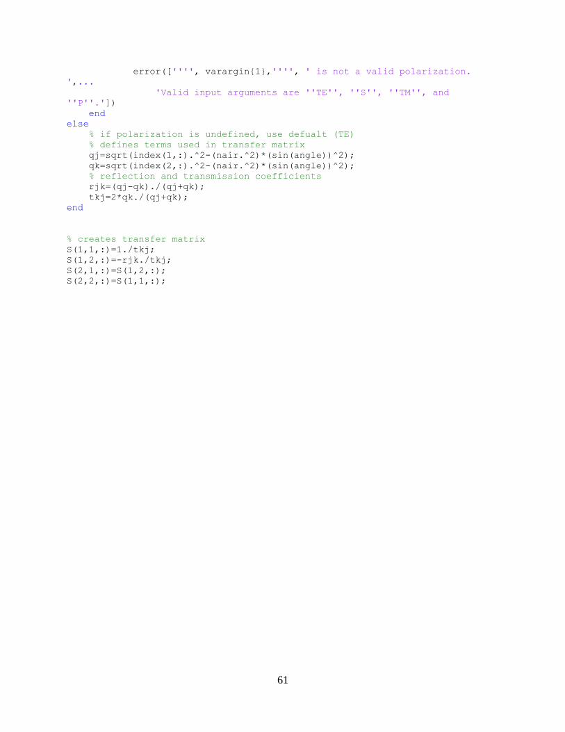
61
error(['''', varargin{1},'''', ' is not a valid polarization.
',...
'Valid input arguments are ''TE'', ''S'', ''TM'', and
''P''.'])
end
else
% if polarization is undefined, use defualt (TE)
% defines terms used in transfer matrix
qj=sqrt(index(1,:).^2-(nair.^2)*(sin(angle))^2);
qk=sqrt(index(2,:).^2-(nair.^2)*(sin(angle))^2);
% reflection and transmission coefficients
rjk=(qj-qk)./(qj+qk);
tkj=2*qk./(qj+qk);
end
% creates transfer matrix
S(1,1,:)=1./tkj;
S(1,2,:)=-rjk./tkj;
S(2,1,:)=S(1,2,:);
S(2,2,:)=S(1,1,:);

62
BIBLIOGRAPHY
(1) Lakowicz, J. R. Principles of Fluorescence Spectroscopy 3rd Ed., 3rd ed.; Springer US,
2006. https://doi.org/10.1007/978-0-387-46312-4.
(2) Forster, T. No Title. Z. Naturforsch. A 1949, 4, 321.
(3) Sapsford, K. E.; Berti, L.; Medintz, I. L.; As, T.; Resonance, F.; Transfer, E.; Dot, Q.;
Biology, M.; Imaging, C. Fluorescence Resonance Energy Transfer. Minerva Biotecnol.
2004, 16 (4), 253–279.
(4) Scholes, G. D. Long-Range Resonance Energy Transfer in Molecular Systems. Annu. Rev.
Phys. Chem. 2003, 54 (1), 57–87.
https://doi.org/10.1146/annurev.physchem.53.082201.124330.
(5) van Grondelle, R.; Dekker, J. P.; GillBro, T.; Sundstorm, V. Energy Transfer and Trapping
in Photosynthesis. Biochim. Biophys. Acta 1994, 1187, 1–65.
(6) Hardin, B. E.; Hoke, E. T.; Armstrong, P. B.; Yum, J.-H.; Comte, P.; Torres, T.; Fréchet, J.
M. J.; Nazeeruddin, M. K.; Grätzel, M.; McGehee, M. D. Increased Light Harvesting in
Dye-Sensitized Solar Cells with Energy Relay Dyes. Nat. Photonics 2009, 3 (7), 406–411.
https://doi.org/10.1038/nphoton.2009.96.
(7) Menke, S. M.; Luhman, W. a; Holmes, R. J. Tailored Exciton Diffusion in Organic
Photovoltaic Cells for Enhanced Power Conversion Efficiency. Nat. Mater. 2013, 12 (2),
152–157. https://doi.org/10.1038/nmat3467.
(8) Baldo, M. A.; O ’Brien, D. F.; You, Y.; Shoustikov, A.; Sibley, S.; Thompson, M. E.;
Forrest, S. R. Highly Efficient Phosphorescent Emission from Organic Electroluminescent
Devices. Nature 1998, 395 (September), 151–154. https://doi.org/10.1038/25954.
(9) Novotny, L.; Hecht, B. Principles of Nano Optics; Cambridge University Press, 2006.
(10) Raether, H. Surface Plasmons on Smooth and Rough Surfaces and on Gratings; Springer:
Berlin, 1988.
(11) Kretschmann, E.; Raether, H. No Title. Z. Naturforsch. A 1968, 23, 2135.
(12) Poddubny, A.; Iorsh, I.; Belov, P.; Kivshar, Y. Hyperbolic Metamaterials. Nat. Photonics
2013, 7 (12), 948–957. https://doi.org/10.1038/nphoton.2013.243.
(13) Krishnamoorthy, H. N. S.; Jacob, Z.; Narimanov, E.; Kretzschmar, I.; Menon, V. M.
Topological Transitions in Metamaterials. Science 2012, 336 (6078), 205–209.
https://doi.org/10.1126/science.1219171.
(14) Törmä, P.; Barnes, W. L. Strong Coupling between Surface Plasmon Polaritons and
Emitters. arXiv 2014, 013901, 1405.1661. https://doi.org/10.1088/0034-4885/78/1/013901.
(15) Novotny, L. Strong Coupling, Energy Splitting, and Level Crossings: A Classical
Perspective. Am. J. Phys. 2010, 78 (11), 1199. https://doi.org/10.1119/1.3471177.
(16) Jaynes, E. T.; Cummings, F. W. Comparison of Quantum and Semiclassical Radiation
63
Theories with Application to the Beam Maser. Proc. IEEE 1963, 51, 89–109.
(17) Martínez-Martínez, L. A.; Ribeiro, R. F.; Campos-González-Angulo, J.; Yuen-Zhou, J. Can
Ultrastrong Coupling Change Ground State Chemical Reactions? 2017, 1–12.
https://doi.org/10.1021/acsphotonics.7b00610.
(18) Lucarini, V.; Saarinen, J. J.; Peiponen, K.-E.; Vartiainen, E. M. Kramers-Kronig Relations
in Optical Materials Research; Springer, 2005.
(19) Andrew, P.; Barnes, W. L. Förster Energy Transfer in an Optical Microcavity. Science (80-
. ). 2000, 290 (5492), 785–788. https://doi.org/10.1126/science.290.5492.785.
(20) Andrew, P.; Barnes, W. L. Energy Transfer across a Metal Film Mediated by Surface
Plasmon Polaritons. Science (80-. ). 2004, 306 (2004), 1002–1005.
https://doi.org/10.1126/science.1102992.
(21) Martín-Cano, D.; Martín-Moreno, L.; García-Vidal, F. J.; Moreno, E. Resonance Energy
Transfer and Superradiance Mediated by Plasmonic Nanowaveguides. Nano Lett. 2010, 10
(8), 3129–3134. https://doi.org/10.1021/nl101876f.
(22) De Torres, J.; Ferrand, P.; Colas Des Francs, G.; Wenger, J. Coupling Emitters and Silver
Nanowires to Achieve Long-Range Plasmon-Mediated Fluorescence Energy Transfer. ACS
Nano 2016, 10 (4), 3968–3976. https://doi.org/10.1021/acsnano.6b00287.
(23) Bouchet, D.; Cao, D.; Carminati, R.; De Wilde, Y.; Krachmalnicoff, V. Long-Range
Plasmon-Assisted Energy Transfer between Fluorescent Emitters. Phys. Rev. Lett. 2016,
116 (3), 037401. https://doi.org/10.1103/PhysRevLett.116.037401.
(24) Ren, J.; Wu, T.; Yang, B.; Zhang, X. Simultaneously Giant Enhancement of Förster
Resonance Energy Transfer Rate and Efficiency Based on Plasmonic Excitations. Phys.
Rev. B - Condens. Matter Mater. Phys. 2016, 94, 125416.
https://doi.org/10.1103/PhysRevB.94.125416.
(25) Biehs, S.-A.; Menon, V. M.; Agarwal, G. S. Long-Range Dipole-Dipole Interaction and
Anomalous F¨ Orster Energy Transfer across a Hyperbolic Metamaterial. Phys. Rev. B -
Condens. Matter Mater. Phys. 2016, 93 (24), 245439.
https://doi.org/10.1103/PhysRevB.93.245439.
(26) Logeeswaran, V. J.; Kobayashi, N. P.; Islam, M. S.; Wu, W.; Chaturvedi, P.; Fang, N. X.;
Wang, S. Y.; Williams, R. S. Ultrasmooth Silver Thin Films Deposited with a Germanium
Nucleation Layer. Nano Lett. 2009, 9 (1), 178–182. https://doi.org/10.1021/nl8027476.
(27) Newman, W. D.; Cortes, C. L.; Afshar, A.; Cadien, K.; Meldrum, A.; Fedosejevs, R.; Jacob,
Z. Observation of Long-Range Dipole-Dipole Interactions in Hyperbolic Metamaterials.
Sci. Adv. 2018, 4 (October), eaar5278. https://doi.org/10.1126/sciadv.aar5278.
(28) Zhong, X.; Chervy, T.; Wang, S.; George, J.; Thomas, A.; Hutchison, J. A.; Devaux, E.;
Genet, C.; Ebbesen, T. W. Non-Radiative Energy Transfer Mediated by Hybrid Light-
Matter States. Angew. Chemie - Int. Ed. 2016, 55 (21), 6202–6206.
https://doi.org/10.1002/anie.201600428.
(29) Coles, D. M.; Somaschi, N.; Michetti, P.; Clark, C.; Lagoudakis, P. G.; Savvidis, P. G.;
64
Lidzey, D. G. Polariton-Mediated Energy Transfer between Organic Dyes in a Strongly
Coupled Optical Microcavity. Nat. Mater. 2014, 13 (7), 712–719.
https://doi.org/10.1038/nmat3950.
(30) Pustovit, V. N.; Urbas, A. M.; Shahbazyan, T. V. Energy Transfer in Plasmonic Systems.
J. Opt. (United Kingdom) 2014, 16 (11). https://doi.org/10.1088/2040-8978/16/11/114015.
(31) Li, J.; Cushing, S. K.; Meng, F.; Senty, T. R.; Bristow, A. D.; Wu, N. Plasmon-Induced
Resonance Energy Transfer for Solar Energy Conversion. Nat. Photonics 2015, 9 (9), 601–
607. https://doi.org/10.1038/nphoton.2015.142.
(32) Jang, S. J.; Mennucci, B. Delocalized Excitons in Natural Light-Harvesting Complexes.
Rev. Mod. Phys. 2018, 90 (3), 35003. https://doi.org/10.1103/RevModPhys.90.035003.
(33) Strümpfer, J.; Sener, M.; Schulten, K. How Quantum Coherence Assists Photosynthetic
Light Harvesting. J. Phys. Chem. Lett. 2012, 3 (4), 536–542.
https://doi.org/10.1021/jz201459c.
(34) Zhong, X.; Chervy, T.; Zhang, L.; Thomas, A.; George, J.; Genet, C.; Hutchison, J. A.;
Ebbesen, T. W. Energy Transfer between Spatially Separated Entangled Molecules. Angew.
Chemie - Int. Ed. 2017, 56, 9034–9038. https://doi.org/10.1002/anie.201703539.
(35) Du, M.; Martínez-Martínez, L. A.; Ribeiro, R. F.; Hu, Z.; Menon, V. M.; Yuen-Zhou, J.
Theory for Polariton-Assisted Remote Energy Transfer. Chem. Sci. 2018, 9 (32), 6659–
6669. https://doi.org/10.1039/c8sc00171e.
(36) Zhang, X.; Marocico, C. A.; Lunz, M.; Gerard, V. A.; Gun’Ko, Y. K.; Lesnyak, V.;
Gaponik, N.; Susha, A. S.; Rogach, A. L.; Bradley, A. L. Experimental and Theoretical
Investigation of the Distance Dependence of Localized Surface Plasmon Coupled Förster
Resonance Energy Transfer. ACS Nano 2014, 8 (2), 1273–1283.
https://doi.org/10.1021/nn406530m.
(37) Hutchison, J. A.; Schwartz, T.; Genet, C.; Devaux, E.; Ebbesen, T. W. Modifying Chemical
Landscapes by Coupling to Vacuum Fields. Angew. Chemie - Int. Ed. 2012, 51 (7), 1592–
1596. https://doi.org/10.1002/anie.201107033.
(38) Galego, J.; Garcia-Vidal, F. J.; Feist, J. Suppressing Photochemical Reactions with
Quantized Light Fields. Nat. Commun. 2016, 7, 1–6.
https://doi.org/10.1038/ncomms13841.
(39) Herrera, F.; Spano, F. C. Cavity-Controlled Chemistry in Molecular Ensembles. Phys. Rev.
Lett. 2016, 116 (June), 238301. https://doi.org/10.1103/PhysRevLett.116.238301.
(40) Shalabney, A.; George, J.; Hutchison, J. a.; Pupillo, G.; Genet, C.; Ebbesen, T. W. Coherent
Coupling of Molecular Resonators with a Microcavity Mode. Nat. Commun. 2015, 6 (Umr
7006), 5981. https://doi.org/10.1038/ncomms6981.
(41) Lochbrunner, S.; Schultz, T.; Schmitt, M.; Shaffer, J. P.; Zgierski, M. Z.; Stolow, A.
Dynamics of Excited-State Proton Transfer Systems via Time-Resolved Photoelectron
Spectroscopy. J. Chem. Phys. 2001, 114 (6), 2519–2522.
https://doi.org/10.1063/1.1345876.
65
(42) Hsieh, C. C.; Chou, P. T.; Shih, C. W.; Chuang, W. T.; Chung, M. W.; Lee, J.; Joo, T.
Comprehensive Studies on an Overall Proton Transfer Cycle of the Ortho -Green
Fluorescent Protein Chromophore. J. Am. Chem. Soc. 2011, 133 (9), 2932–2943.
https://doi.org/10.1021/ja107945m.
(43) Sarker, N.; Das, K.; Das, S.; Datta, A.; Nath, D.; Bhattacharyya, K. Excited-State
Intramolecular Proton Transfer of 2-(2’-Hydroxyphenyl)Benzimidazole in Micelles. J.
Phys. Chem. 1995, 99 (50), 17711–17714. https://doi.org/10.1021/j100050a007.
(44) Barbara, P. F.; Walsh, P. K.; Brus, L. E. Picosecond Kinetic and Vibrationally Resolved
Spectroscopic Studies of Intramolecular Excited-State Hydrogen Atom Transfer. J. Phys.
Chem. 1989, 93 (1), 29–34. https://doi.org/10.1021/j100338a011.
(45) Hsieh, C. C.; Jiang, C.-M.; Chou, P. T. Recent Experimental Advances on Excited-State
Intramolecular Proton Coupled Electron Transfer Reaction. Acc. Chem. Res. 2010, 43 (10),
1364–1374.
(46) Wu, J.; Liu, W.; Ge, J.; Zhang, H.; Wang, P. New Sensing Mechanisms for Design of
Fluorescent Chemosensors Emerging in Recent Years. Chem. Soc. Rev. 2011, 40 (7), 3483–
3495. https://doi.org/10.1039/c0cs00224k.
(47) Chen, K. Y.; Hsieh, C. C.; Cheng, Y. M.; Lai, C. H.; Chou, P. T. Extensive Spectral Tuning
of the Proton Transfer Emission from 550 to 675 Nm via a Rational Derivatization of 10-
Hydroxybenzo[h]Quinoline. Chem. Commun. 2006, 1 (42), 4395–4397.
https://doi.org/10.1039/b610274c.
(48) Tang, K. C.; Chang, M. J.; Lin, T. Y.; Pan, H. A.; Fang, T. C.; Chen, K. Y.; Hung, W. Y.;
Hsu, Y. H.; Chou, P. T. Fine Tuning the Energetics of Excited-State Intramolecular Proton
Transfer (ESIPT): White Light Generation in a Single ESIPT System. J. Am. Chem. Soc.
2011, 133 (44), 17738–17745. https://doi.org/10.1021/ja2062693.
(49) Kwon, J. E.; Park, S. Y. Advanced Organic Optoelectronic Materials: Harnessing Excited-
State Intramolecular Proton Transfer (ESIPT) Process. Adv. Mater. 2011, 23 (32), 3615–
3642. https://doi.org/10.1002/adma.201102046.
(50) Padalkar, V. S.; Seki, S. Excited-State Intramolecular Proton-Transfer (ESIPT)-Inspired
Solid State Emitters. Chem. Soc. Rev. 2016, 45 (1), 169–202.
https://doi.org/10.1039/c5cs00543d.
(51) Galego, J.; Garcia-Vidal, F. J.; Feist, J. Cavity-Induced Modifications of Molecular
Structure in the Strong-Coupling Regime. Phys. Rev. X 2015, 5 (4), 041022.
https://doi.org/10.1103/PhysRevX.5.041022.
(52) Raizen, M. G.; Thompson, R. J.; Brecha, R. J.; Kimble, H. J.; Carmichael, H. J. Normal-
Mode Splitting and Linewidth Averaging for Two-State Atoms in an Optical Cavity. Phys.
Rev. Lett. 1989, 63 (3), 240–243. https://doi.org/10.1103/PhysRevLett.63.240.
(53) Thompson, R. J.; Rempe, G.; Kimble, H. J. Observation of Normal-Mode Splitting for an
Atom in an Optical Cavity. Phys. Rev. Lett. 1992, 68 (8), 1132–1135.
(54) Weisbuch, C.; Nishioka, M.; Ishikawa, A.; Arakawa, Y. Observation of the Coupled
Exciton-Photon Mode Splitting in a Semiconductor Quantum Microcavity. Phys. Rev. Lett.
66
1992, 69 (23), 3314–3317.
(55) Skolnick, M. S.; Fisher, T. A.; Whittaker, D. M. Strong Coupling Phenomena in Quantum
Microcavity Structures - Abstract - Semiconductor Science and Technology - IOPscience.
1998.
(56) Holmes, R. J.; Forrest, S. R. Strong Exciton-Photon Coupling and Exciton Hybridization in
a Thermally Evaporated Polycrystalline Film of an Organic Small Molecule. Phys. Rev.
Lett. 2004, 93 (October), 186404. https://doi.org/10.1103/PhysRevLett.93.186404.
(57) Holmes, R. J.; Forrest, S. R. Strong Exciton-Photon Coupling in Organic Materials. Org.
Electron. 2007, 8 (2–3), 77–93. https://doi.org/10.1016/j.orgel.2006.05.005.
(58) Lidzey, D. G.; Bradley, D. D. C.; Skolnick, M. S.; Virgili, T.; Walker, S.; Whittaker, D. M.
Strong Exciton-Photon Coupling in an Organic Semiconductor Microcavity. Nature 1998,
395 (6697), 53–55. https://doi.org/10.1038/25692.
(59) Plumhof, J. D.; Stöferle, T.; Mai, L.; Scherf, U.; Mahrt, R. F. Room-Temperature Bose-
Einstein Condensation of Cavity Exciton-Polaritons in a Polymer. Nat. Mater. 2013, 13 (4),
247–252. https://doi.org/10.1038/nmat3925.
(60) Lerario, G.; Fieramosca, A.; Barachati, F.; Ballarini, D.; Daskalakis, K. S.; Dominici, L.;
De Giorgi, M.; Maier, S. A.; Gigli, G.; Kéna-Cohen, S.; et al. Room-Temperature
Superfluidity in a Polariton Condensate. 2017, 13 (September), 837–842.
https://doi.org/10.1038/nphys4147.
(61) Törmä, P.; Barnes, W. L. Strong Coupling between Surface Plasmon Polaritons and
Emitters : A Review. Reports Prog. Phys. 2015, 78, 13901. https://doi.org/10.1088/0034-
4885/78/1/013901.
(62) Kéna-Cohen, S.; Forrest, S. R. Giant Davydov Splitting of the Lower Polariton Branch in a
Polyerystalline Tetracene Microcavity. Phys. Rev. B - Condens. Matter Mater. Phys. 2008,
77, 073205. https://doi.org/10.1109/LEOS.2007.4382308.
(63) Herrera, F.; Spano, F. C. Dark Vibronic Polaritons and the Spectroscopy of Organic
Microcavities. Phys. Rev. Lett. 2017, 118 (22), 223601–1.
https://doi.org/10.1103/PhysRevLett.118.223601.
(64) Nichols, V. M.; Broch, K.; Schreiber, F.; Bardeen, C. J. Excited-State Dynamics of
Diindenoperylene in Liquid Solution and in Solid Films. 2015.
https://doi.org/10.1021/acs.jpcc.5b03353.
(65) Hakala, T. K.; Toppari, J. J.; Kuzyk, a.; Pettersson, M.; Tikkanen, H.; Kunttu, H.; Törmä,
P. Vacuum Rabi Splitting and Strong-Coupling Dynamics for Surface-Plasmon Polaritons
and Rhodamine 6G Molecules. Phys. Rev. Lett. 2009, 103 (July), 1–4.
https://doi.org/10.1103/PhysRevLett.103.053602.
(66) Bellessa, J.; Bonnand, C.; Plenet, J. C.; Mugnier, J. Strong Coupling between Surface
Plasmons and Excitons in an Organic Semiconductor. Phys. Rev. Lett. 2004, 93 (3), 036404-
1. https://doi.org/10.1103/PhysRevLett.93.036404.
(67) Symonds, C.; Bonnand, C.; Plenet, J. C.; Bréhier, A.; Parashkov, R.; Lauret, J. S.; Deleporte,
67
E.; Bellessa, J. Particularities of Surface Plasmon-Exciton Strong Coupling with Large Rabi
Splitting. New J. Phys. 2008, 10. https://doi.org/10.1088/1367-2630/10/6/065017.
(68) Heilig, M. Ã.; Domhan, M.; Port, H. Optical Properties and Morphology of Thin
Diindenoperylene Films. 2004, 110, 290–295.
https://doi.org/10.1016/j.jlumin.2004.08.023.
(69) Zhang, D.; Horneber, A.; Mihaljevic, J.; Heinemeyer, U.; Braun, K.; Schreiber, F.; Scholz,
R.; Meixner, A. J. Plasmon Resonance Modulated Photoluminescence and Raman
Spectroscopy of Diindenoperylene Organic Semiconductor Thin Film. J. Lumin. 2011, 131
(3), 502–505. https://doi.org/10.1016/j.jlumin.2010.09.008.