Contributions of Internal Variability and External Forcing to the Recent Trends in theSoutheastern Pacific and Peru–Chile Upwelling System

BEYREM JEBRI, MYRIAM KHODRI, VINCENT ECHEVIN, GUILLAUME GASTINEAU, SYLVIE THIRIA,JÉROME VIALARD, AND NICOLAS LEBAS

LOCEAN-IPSL, Sorbonne-Université, CNRS/IRD/UPMC/MNHN, Paris, France

(Manuscript received 25 April 2019, in final form 30 December 2019)

ABSTRACT

In a warming world context, sea surface temperature (SST) off central-south Peru, northern Chile, and

farther offshore increases at a slower rate than the global average since several decades (i.e., cools, relative to

the global average). This tendency is synchronous with an interdecadal Pacific oscillation (IPO) negative

trend since;1980, which has a cooling signature in the southeastern Pacific. Here, we use a large ensemble of

historical coupled model simulations to investigate the relative roles of internal variability (and in particular

the IPO) and external forcing in driving this relative regional cooling, and the associated mechanisms. The

ensemble mean reproduces the relative cooling, in response to an externally forced southerly wind anomaly,

which strengthens the upwelling off Chile in recent decades. This southerly wind anomaly results from the

poleward expansion of the Southern Hemisphere Hadley cell. Attribution experiments reveal that this

poleward expansion and the resulting enhanced upwelling mostly occur in response to increasing greenhouse

gases and stratospheric ozone depletion since ;1980. An oceanic heat budget confirms that the wind-forced

upwelling enhancement dominates the relative cooling near the coast. In contrast, a wind-forced deepening of

the mixed layer drives the offshore cooling. While internal variability contributes to the spread of tendencies,

the ensemble-mean relative cooling in the southeastern Pacific is consistent with observations and occurs

irrespectively of the IPO phase, hence, indicating the preeminent role of external forcing.

1. Introduction

The Humboldt Peru–Chile upwelling system (PCUS;

Strub et al. 1998) is one of the most productive oceanic

regions globally in terms of phytoplankton (Chavez

et al. 2008; Kämpf and Chapman 2016) and represents

one of the leading fisheries in the world, thriving with

high biological diversity (Cushing 1971; Fréon et al.

2009). As in other eastern boundary upwelling systems,

alongshore equatorward wind stress and the associated

wind stress curl drive coastal upwelling. The action of

the surface wind stress pushes surface waters offshore

and pumps up deeper, cold, and nutrient-rich waters

(Sverdrup 1938), triggering the high surface productiv-

ity. Ecosystems and fisheries are already under strong

pressure from climate change globally, with projections

pointing to an overall oceanic warming, acidification,

deoxygenation, and reduced primary productivity (e.g.,

Bopp et al. 2013, Beaugrand et al. 2019). Due to the

strong socioeconomic relevance of the PCUS (Ibarra

et al. 2000; Pérez et al. 2010), it is critical to further in-

vestigate and quantify the potential impacts of climate

change in this region.

Previous works documenting the PCUS long-term

upwelling trends have mostly relied on wind stress

based upwelling indices over recent decades (e.g., Aravena

et al. 2014) or estimates from phase 5 of the Coupled

Model Intercomparison Project (CMIP5) global circula-

tion models to infer wind-driven upwelling intensity vari-

ations into the twenty-first century (e.g., Rykaczewski et al.

2015; Wang et al. 2015). Analyses from general circulation

models have suggested mixed results and even con-

tradictory trends for the Humboldt system (Oyarzúnand Brierley 2019). On the other hand, sea surface

temperature (SST) cooling trends (Figs. 1a,b) have

been observed off Chile since the 1980s (Falvey and

Garreaud 2009) and off central-south Peru since the

1950s (Gutiérrez et al. 2011). These coastal trends havebeen interpreted as an indirect evidence of wind-driven

upwelling intensification.

Denotes content that is immediately available upon publica-

tion as open access.

Corresponding author: Beyrem Jebri, beyrem.jebri@locean-ipsl.

upmc.fr

15 DECEMBER 2020 J EBR I ET AL . 10555

DOI: 10.1175/JCLI-D-19-0304.1

� 2020 American Meteorological Society. For information regarding reuse of this content and general copyright information, consult the AMS CopyrightPolicy (www.ametsoc.org/PUBSReuseLicenses).

Unauthenticated | Downloaded 02/26/22 12:24 PM UTC

Low-frequency SST changes in this region can also be

associated with internal climate variability (Montecinos

et al. 2003; Vargas et al. 2007). While El Niño–SouthernOscillation (ENSO; e.g., McPhaden et al. 2006) is the

leading mode of interannual climate variability in the

Pacific Ocean, its decadal fluctuations imprint a pan-

Pacific pattern of coherent SST decadal variability

(Newman et al. 2016) through atmospheric teleconnections

(e.g., Alexander et al. 2002). This pattern is known as the

interdecadal Pacific oscillation (IPO), and is the leading

mode of internal, decadal to multidecadal variability in

the PacificOcean (Folland et al. 1999; Power et al. 1999).

The IPO SST pattern is broadly similar to that of ENSO,

but less equatorially confined in the eastern Pacific and

more prominent in the extratropical latitudes (Minobe

1997; Minobe 1999; Deser et al. 2004; Deser et al. 2010).

The IPO has experienced a trend from a positive (i.e., El

Niño–like) to a negative (La Niña–like) phase over the

1980–2014 period (Fig. 1c), associated with an intensi-

fication of Pacific trade winds and with a shoaling of

the thermocline in the eastern equatorial Pacific (e.g.,

Balmaseda et al. 2013; de Boisséson et al. 2014; England

et al. 2014; Kociuba and Power 2015; Choi et al. 2016;

Gastineau et al. 2018). Poleward propagating coastal

waves and a shoaling of the nearshore thermocline may

also play a key role in modulating SST at decadal time

scales off Chile (e.g., Montecinos et al. 2007). Such an

IPO phase transition during the 1980–2014 period is

indeed associated with a central and eastern equatorial

Pacific cooling that extends toward midlatitudes and in

particular into the southeastern Pacific (hereafter, SEP)

and the broad PCUS region (Figs. 1a,b). Thus, the IPO

might have contributed to the recent cooling trend in

this region.

Nevertheless, the PCUS trends over recent decades

could also result from external forcing. Under green-

house gas forcing continental surface temperatures in-

crease more than nearby SSTs because of the drier

environment and larger lapse-rate over land (e.g., Joshi

et al. 2008; Dommenget 2009). This lowers pressure over

land (e.g., Bayr and Dommenget 2013) and potentially

strengthens the land–sea sea level pressure gradient and

the upwelling-favorable alongshore wind stress (Bakun

et al. 2010). Indeed, CMIP5model projections point to a

FIG. 1. Sea surface temperature trend in austral summer (December–February) for the period 1980–2014,

in 8Cdecade21 for (a) ERSSTv4, (b) ERA-Interim, and (d) ALL ensemble mean. Stippling denotes regions where

the observed or ensemble mean trend is significant at the 90% confidence level. The black contour lines in

(d) indicate where at least 90% of the ALL ensemble members have a positive sea surface temperature trend.

(c) IPO TPI index from ERSSTv4 dataset. The green curve shows the ALL ensemble-mean IPO index. The purple

dashed line corresponds to the 1980–2014 IPO index linear trend from ERSSTv4.

10556 JOURNAL OF CL IMATE VOLUME 33

Unauthenticated | Downloaded 02/26/22 12:24 PM UTC

significant increase in the duration and intensity of

upwelling-favorable winds in the poleward portions

of the fourmajor eastern boundary upwellings (California,

Canary, Humboldt, Benguela), which highly correlates to

the land–sea temperature gradient (Wang et al. 2015).

The alongshore winds intensification is, however, not

accompanied by a clear reinforcement of the land low

pressure system either in CMIP5 historical simulations

or in projections (Rykaczewski et al. 2015). Belmadani

et al. (2014) suggest that the enhancement of upwelling-

favorable winds over the PCUS are rather due to sub-

tropical southerly wind anomalies linked to a poleward

expansion of the Southern Hemisphere Hadley cell

(HC). Several observational datasets and reanalyses

indeed show that the Southern Hemisphere HC southern

edge (;208S in the current climate) has shifted southward

by about 0.38–0.58 of latitude per decade since 1979

(Johanson and Fu 2009; Hu et al. 2011, 2013; Choi et al.

2014; Staten et al. 2018; Grise et al. 2019), with the largest

poleward expansion during austral summer (Chen et al.

2014). Climate model experiments suggest that the HC

poleward expansion is forced by the ozone depletion

from 1979 to the late 1990s (e.g., Son et al. 2010;

McLandress et al. 2011; Hu et al. 2013; Min and Son

2013) and by the rising concentration of atmospheric

greenhouse gases (Lu et al. 2007; Staten et al. 2012;

Quan et al. 2014; Adam et al. 2014). However, the

tendency toward more La Niñas in relation with the

recent IPO trend may also contribute to the HC pole-

ward shift (Nguyen et al. 2013).

To our knowledge, previous studies have not specifi-

cally examined (i) the respective role of anthropogenic

forcing and internal climate variability in long-term

trends in the PCUS, (ii) the specific role of the HC ex-

pansion on PCUS changes and its attribution to specific

sources of external forcing, and (iii) the physical pro-

cesses responsible for the weak SST warming in the

southeastern Pacific (relative to the global mean) over

the last decades. These are the questions addressed in

this study. Here, we assess the 1940–2020 PCUS climate

changes, using observations and a set of 20–30-member

ensembles conductedwith the IPSL-CM5A-LR (Dufresne

et al. 2013) coupled general circulation model. The

paper is organized as follows: in section 2, we describe

the model, data, and methods. Section 3 presents the

globally averaged SST trends in the model, and then

focuses on the PCUS region, for a validation of the

ensemble-mean climatology and overview of the en-

semble trends. In section 4, we explore the relative

roles of externally forced versus internal variability.

Section 5 describes the contribution of various exter-

nal forcing (greenhouse gases, stratospheric ozone,

volcanoes) on the Hadley cell expansion and PCUS.

In section 6, we investigate the mechanisms responsi-

ble for the relative SST cooling in the southeastern Pacific.

Results are discussed in section 7 before concluding.

2. Methods and data

a. The coupled model

We used the CMIP5 version of the Institut Pierre-

Simon Laplace (IPSL) atmosphere–ocean general cir-

culation model, called IPSL-CM5A-LR (Dufresne et al.

2013). LR stands for low resolution, as the atmospheric

grid resolution is 1.878 in latitude and 3.758 in longitude. It

includes the LMDZ5A atmospheric component (Hourdin

et al. 2013), with 39 hybrid sigma-pressure levels, in-

cluding 15 in the stratosphere. LMDZ5A is coupled to

the ORCHIDEE (Krinner et al. 2005) land surface

component. The oceanic component uses Nucleus for

European Modelling of the Ocean (NEMO), version

3.2 (Madec 2008), with 31 vertical levels (and resolu-

tion decreasing from 10m near the surface to 500m

toward the bottom), a mean spatial horizontal resolu-

tion of about 28 (with a refinement to a 0.58 latitudinalresolution near the equator). The oceanmodel includes

the LIM2 sea ice model (Fichefet and Maqueda 1997).

Compared to other CMIP5 models, IPSL-CM5A-LR

has a relatively large transient climate response, reach-

ing 2K per CO2 doubling. It thus ranks among the high-

sensitivity climate models of CMIP5 (multimodel mean

of 1.82 6 0.63K) (Andrews et al. 2012; Forster et al.

2013), due to a large positive low-level clouds feedback

(Brient and Bony 2013). Previous works show that this

model reproduces ENSO variability with two spectral

peaks around 3–3.5 years and beyond 4 years, which is in

good qualitative agreement with observations (Bellenger

et al. 2014). IPSL-CM5A-LR is also realistic for other

aspects of the climate variability. It simulates well the

characteristics of observed North Pacific variability

(Fleming and Anchukaitis 2016) and the links between

ENSO and the IPO (Nidheesh et al. 2017). However,

like many global climate models, IPSL-CM5A-LR

simulates a double intertropical convergence zone

(ITCZ) and the classical cold tongue bias in the Pacific

(Dufresne et al. 2013). The observed ENSO seasonal

phase locking is also not well captured (Bellenger et al.

2014). Last, IPSL-CM5A-LR also has a rather strong

cold bias for the surface air temperature, in particular

in the midlatitudes.

b. Experimental protocol

We performed four IPSL-CM5A-LR ensembles with

historical external forcing for the 1940–2020 period (see

Table 1). The first ensemble of 30 members (referred

to as the ALL ensemble) uses the historical CMIP5

15 DECEMBER 2020 J EBR I ET AL . 10557

Unauthenticated | Downloaded 02/26/22 12:24 PM UTC

(Taylor et al. 2012) concentrations of greenhouse gases

(GHG) from 1940 to 2005 and from RCP8.5 between

2006 and 2020 (Riahi et al. 2011). The standard CMIP5

ozone concentration used in IPSL-CM5A-LR was cal-

culated from a separate atmospheric simulation with

interactive atmospheric chemistry (Szopa et al. 2013).

We also use the historical stratospheric aerosol forcing

from the main volcanic eruptions by prescribing the

aerosol optical depth, as given in Sato et al. (1993) (2012

updated version).

Three other ensembles use each forcing individually,

namely either volcanic (referred to as VOLC), green-

house gases (referred to as GHG), or ozone (referred to

as OZ) forcing, while maintaining other forcing at their

1940 level. The VOLC, GHG, and OZ ensembles have

20 members each. Each ensemble member starts in

January 1940 from randomly sampled initial conditions

(31 December) chosen over 1920–60 in a set of IPSL-

CM5A CMIP5 historical simulations (initiated in 1870)

using all forcings (i.e., similar to ALL). Tropospheric

aerosols forcing is maintained to the preindustrial level

in all simulations.

Taking initial conditions that sample random phases

of the internal climate variability guarantees that this

variability is largely uncorrelated across members from

the start of the experiments. The ensemble averaging of

the large number of members hence damps the internal

climate variability by a factor of On in a n-member en-

semble, so that it is reduced by a factor of;5.5 and 4.5 in

the 30- and 20-member ensembles, respectively. It al-

lows effective isolation of the externally forced vari-

ability. This is demonstrated in Fig. 1c, which shows the

ALL ensemble mean IPO index (green curve) whose

variability is much smaller than the observed one,

confirming that the large ensemble averaging success-

fully damps out internal variability.

c. Trend analysis and statistical testing

All anomalies are calculated by removing the 1941–

61 monthly mean seasonal cycle to the time series. We

then applied a Hanning filter with a 7-yr cutoff period to

focus only on the decadal variability. All the linear

trends in the paper are computed from the low-pass-

filtered time series, using least squares. On time series

plots, the ensemble mean is plotted, along with an esti-

mate of the intermember spread. Depending on the

figure, this spread is either estimated from the 5th and

95th percentiles or from the 90% confidence interval,

assuming Gaussian distributions and considering each

member as independent. Trendmaps are computed over

1980–2014 and regions where the trend (ensemble mean

trend for simulations) is significantly different from zero

at 90% confidence level are estimated with a Wald test

using a t distribution for the test statistic. We also indi-

cate regions where more than 60% and 90% of the

members display anomalies of the same sign as the en-

semble mean trend.

d. Upwelling and IPO indices

We considered four main variables to characterize the

variations of the PCUS in each ensemble: meridional

surface wind stress (ty), wind stress curl (z), SST, and

vertical velocity at 100-m depth (w100). Because the re-

gions over which the variability of these variables is

homogenous are not necessarily square boxes, and may

depend on the variable, we have defined specific regions

for each variable according to their covariability. We

defined regions in the broad southeast Pacific region

(108N–528S, 1138–668W) by clustering, for each variable,

nearby grid points with similar temporal variations

based on correlations of their 1940–2020 time series. To

do so we combined the ClustVar (Vigneau and Qannari

2003) algorithms and the self-organizing map (SOM)

(Kohonen 1998) topological ordering proprieties in or-

der to aggregate variables together according to their

covariability. We then extract spatial regions of coher-

ent temporal variability from this clustering. To ana-

lyze the IPO, we use the SST tripole index (TPI; Henley

et al. 2015), defined as the central equatorial Pacific SST

(108S–108N, 1708E2908W) minus the average of north-

west (258–458N, 1408E21458W) and southwest (158–508S,1508E21608W) Pacific SST, smoothed using a 13-yr

Chebyshev low-pass filter.

e. Mixed layer heat budget

We compute a simplified mixed layer heat budget for

each member of the ALL ensemble using monthly data,

in order to quantify the respective contributions of sur-

face heat flux and oceanic processes to the SST ten-

dencies. The mixed layer heat budget is expressed as

follows:

DSST (t)5

ðtt0

"Q

atm(t0)

r3 cp3 h (t0)

#dt0 1OCE

dyn(t) , (1)

TABLE 1. Ensemble size and external forcing considered over the

1940–2020 period for the ensemble IPSL-CM5A-LR experiments

used in this study (see section 2b).

Used external forcing

Experiment

name

Greenhouse

gases Ozone

Volcanic

forcing

Model

members

ALL 3 3 3 30

GHG 3 — — 20

OZ — 3 — 20

VOLC — — 3 20

10558 JOURNAL OF CL IMATE VOLUME 33

Unauthenticated | Downloaded 02/26/22 12:24 PM UTC

with

Qatm

5Qlw1Q

flat1Q

sens1Q

sw2Q

swh, (2)

where DSST(t) is the SST monthly variation between t0(taken as 1950) and t. The first term of the right-hand

side in Eq. (1) represents the SST anomaly due to sur-

face heat flux. The Qatm(t) represents the anomalous

net surface heat flux into the oceanic mixed layer. The

h(t) is the thickness of the mixed layer defined as the

depth at which the vertical eddy diffusivity coefficient

falls below a given value (here taken equal to back-

ground value of 5 cm2 s21) and can be interpreted as a

maximum penetration depth of the turbulent motion

in the surface layer. HereCp and r denote the seawater

specific heat (4000 J kg21 K21) and a reference density

(1025 kgm23), respectively. We compute the first term

on the right-hand side of the equation using monthly

mean averages. The net surface heat flux is composed

of Qsw the shortwave radiative flux at the ocean sur-

face, Qswh the shortwave radiative flux transmitted

through the bottom of the mixed layer, Qlw the long-

wave radiative flux,Qflat the latent heat flux, and Qsens

the sensible heat flux. The net heat flux is defined

positive downward. The second term on the right-hand

side of Eq. (1) is the SST anomaly due to ocean dy-

namics OCEdyn(t) (including the local influence of

upwelling) estimated as a residual. It corresponds to

ocean processes such as the horizontal and vertical ad-

vection of temperature and horizontal and vertical tur-

bulent mixing. Since the ocean dynamical term is

estimated as a residue from the SST change and the

atmospheric heat flux effect, it may also contain errors

associated with neglecting the submonthly variations

of surface heat flux and mixed layer depth when

computing the atmospheric forcing term.

f. Observations and reanalyses

Our study uses global gridded monthly analyses of

NOAAOptimal Interpolation Sea Surface Temperature,

version 2 (OISSTv2; Reynolds et al. 2002), which begins

in December 1981 and ERSSTv4 (Huang et al. 2015),

which starts in 1854. We also analyze the SST seasonal

cycle and the wind stress patterns from SODA2.2.1

Ocean Reanalyses climatology (Carton and Giese 2008),

representative of the 1941–61 period. Last, we use sea

level pressure (SLP), surface wind stress, 2-m air

temperature, 3D wind, and pressure fields (to compute

the atmospheric meridional overturning streamfunction)

from the European Centre for Medium-RangeWeather

Forecasts (ECMWF) ERA-Interim reanalysis (ERA-I)

over 1979–2014 (Dee et al. 2011), twentieth-century

NOAA–CIRES (NOAA-20C; Compo et al. 2011), and

NCEP (Kalnay et al. 1996).

3. Model validation

a. Global warming signal and contributions fromindividual forcing sources

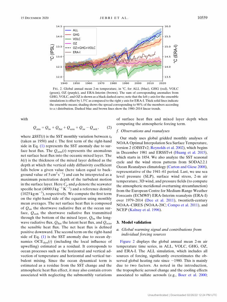
Figure 2 displays the global annual mean 2-m air

temperature time series, in ALL, VOLC, GHG, OZ,

and ERA-I. The ALL simulation, which includes all

sources of forcing, significantly overestimates the ob-

served global heating rate since ;1980. This is mainly

due to two factors. As noted in the introduction,

the tropospheric aerosol change and the cooling effects

associated to sulfate aerosols (e.g., Boer et al. 2000;

FIG. 2. Global annual mean 2-m temperature, in 8C, for ALL (blue), GHG (red), VOLC

(green), OZ (purple), and ERA-Interim (brown). The sum of corresponding anomalies from

GHG, VOLC, andOZ is shown as a black dashed curve; note that the left y axis for the ensemble

simulations is offset by 1.58C as compared to the right y axis for ERA-I. Thick solid lines indicate

the ensemble means; shading shows the spread corresponding to 90% of the members according

to a t distribution. Dashed blue and brown lines show the 1980–2014 linear trends.

15 DECEMBER 2020 J EBR I ET AL . 10559

Unauthenticated | Downloaded 02/26/22 12:24 PM UTC

Allen and Ajoku 2016) are omitted in these simulations

(see section 2b). The overestimated warming also orig-

inates from the large climate sensitivity of IPSL-CM5A-

LR (Forster et al. 2013). Besides, the (GHG1VOLC1OZ) mean 2-m air temperature fits well that of ALL,

suggesting linear additivity of the response to individual

external forcing, in terms of global mean 2-m air tem-

perature anomalies. GHG forcing is clearly the main

driver of the 2-m air temperature increase and explains

most (10.758C) of the 1980–2014 warming trend in ALL

(10.998C), consistent with the behavior of other CMIP5

models (Knutson et al. 2017). Only a weak warming

(10.188C) is simulated in OZ over the period. This

probably reflects the transient adjustment of the climate

system toward a warmer state. It could also be due to

the small increase in tropospheric ozone acting as a

greenhouse gas. VOLC illustrates the strong cooling

contribution to ALL a few years following the three

main historical volcanic eruptions, namely Agung in

1963, El Chichón in 1982, and Pinatubo in 1991. We

further use the GHG, VOLC, and OZ experiments in

section 5c to attribute changes in the PCUS to specific

forcing sources.

b. Global warming trend pattern

The comparison of the ALL ensemble-mean and ob-

served 1980–2014 SST trends reveals large differences

(Figs. 1a,b,d). The two observational products display

significant positive SST trends over the North Atlantic

Ocean, most of the western Indian Ocean, the tropical

and subtropical western Pacific, while weak cooling

trends are observed over much of the eastern equatorial

Pacific. The observed SST trends capture the negative

IPO-like trend pattern (Figs. 1a,b; Deser et al. 2010),

with coastal cooling off California and Chile–Peru (Falvey

andGarreaud 2009;Gutiérrez et al. 2011) and overmost of

the equatorial Pacific. The ensemble averaging in ALL

filters out internal variability such as that of the IPO, hence

reveals the externally forced warming over the period.

As a result, theALL experiment (Fig. 1d) features a large-

scale positive trend, largest in subtropical latitudes (Foster

and Rahmstorf 2011). The lack of tropospheric aerosol

forcing and overestimated climate sensitivity also probably

contribute to the more preeminent warming than in

observations. Despite these differences, the ALL en-

semble mean reveals a weak warming trend over much

of the SEP, the Southern Ocean and the subpolar

Atlantic, consistently with the SST patterns simulated

by most models in response to natural and anthropo-

genic forcing of the twentieth century (e.g., Stouffer

et al. 1989). In particular, no significant SST trend

is simulated off the coasts of central and south Chile

(308–508S). This weak surface warming off Chile can be

interpreted as an indirect evidence of the intensifica-

tion of upwelling in the PCUS in response to the an-

thropogenic forcing, as suggested by Belmadani et al.

(2014),Wang et al. (2015), and Rykaczewski et al. (2015).

c. Peru–Chile upwelling system

In this subsection, we validate the climatological

structure of the PCUS in the ALL experiment. Coastal

upwelling dynamics are very sensitive to the wind stress

structure near the coast (Capet et al. 2004; Small et al.

2015; Renault et al. 2016). Alongshore wind stress at the

coast drives the offshore Ekman transport that leads to

coastal upwelling. The wind stress also weakens when

approaching the coast due to the enhanced friction on

land, generating negative wind stress curl and upward

Ekman pumping (e.g., Belmadani et al. 2014). Despite

its coarse resolution, the model reproduces the first-order

seasonal characteristics of the PCUS, namely the inten-

sification of meridional wind stress, associated coastal

cooling and positive oceanic velocities off Chile (;208–308S) in boreal winter (DJF) and off south Peru (;158–208S) in boreal summer (JJA) (Fig. 3). The known ‘‘cold

tongue’’ bias of coupled climate models (e.g., Li and Xie

2014) is visible in JJA, but does not extend into the PCUS.

d. Hadley circulation

We here diagnose the Hadley circulation in our

model based on the meridional streamfunction. The

meridional streamfunction in ALL (Figs. 4a,b, black

contours) is consistent with results from previous

model studies (Gastineau et al. 2008; Kim et al. 2017)

and reanalyses (Mitas and Clement 2005). We define

the Southern Hemisphere Hadley cell edge as the

linearly interpolated latitude for which the 500-hPa

meridional streamfunction (c500) is equal to zero.

There is an overall good agreement between the ALL

and ERA-I c500 (Fig. 4c) despite a southern edge lo-

cated too much equatorward (2.28 latitude in DJF and

0.98 in JJA) as in other coupled general circulation

models. This discrepancy is linked to the positions of

subtropical jets that are also positioned too close to the

equator (Barnes and Polvani 2013; Arakelian and

Codron 2012).

4. Long-term regional trends and external forcingcontribution

a. Regional trends in the Peru–Chile upwelling system

We already underlined that the broad SEP region

warms less than the global average in the previous sec-

tion. To visualize that signal more clearly, and to get

rid of the overestimated warming in our simulations, we

now examine SST trends relative to the global average

10560 JOURNAL OF CL IMATE VOLUME 33

Unauthenticated | Downloaded 02/26/22 12:24 PM UTC

FIG. 3. Mean climatological sea surface temperature (SST, in 8C) and surface wind stress (t, in

Pa) for the 1941–61 period for (a),(b) SODA2.2.4 and (c),(d)ALLensemblemean, inDecember–

February (DJF) and June–August (JJA), respectively. (e),(f) Mean climatological ocean vertical

velocity at 100-m depth (W100, mday21) over the 1941–61 period for ALL ensemble mean in

DJF and JJA. Red (blue) shading corresponds to upward (downward) velocity.

15 DECEMBER 2020 J EBR I ET AL . 10561

Unauthenticated | Downloaded 02/26/22 12:24 PM UTC

(hereafter relative SST trends, similar to, e.g., Vecchi

and Soden 2007). The ERA-I SST displays an extended

coastal cooling in both seasons (Figs. 5a,b), with a

maximum negative trend off Chile between 358 and 438SinDJF, and off Peru between 108 and 278S in JJA. InALL,

the cooling trend off the South American coast occurs

between 208 and 358S during both seasons (Figs. 5e,f).

Although the cooling trend pattern in ALL broadly agrees

with that of the observed negative SST trend, it is shifted

northward by about 58 in DJF and southward by 58 in JJA.

Consistent and significant southerly (i.e., upwelling-

favorable) wind stress trends develop off Chile in DJF

and off north Chile and south Peru in JJA in ERA-I and

ALL, albeit with a 4 times stronger amplitude in ERA-I.

The amplitude difference is probably related to en-

semble averaging, which damps the internal climate

variability by a factor of On in an n-member ensemble.

Such positive wind stress trends are, however, located at

the poleward boundaries of their climatological pattern,

suggesting a southward extension of the southerly wind

regime, in agreement with other CMIP5 climate change

projections (Rykaczewski et al. 2015; Wang et al. 2015).

FIG. 4. Mean meridional streamfunction, in 1010 kg s21, positive clockwise, for (a) DJF and (b)

JJA for theALL ensemble mean. The black contour corresponds to the climatological values with

contours every 23 1010 kg s21. The color shading shows the trend in 1010 kg s21 per decade for the

1980–2014 period. Stippling denotes regions where at least 90% of the ensemble members have

anomalies of the same sign. The horizontal dashed lines locate the 500-hPa level. (c),(d) Mean

climatological meridional streamfunction at 500 hPa (c500) for the 1941–61 period for ALL (thick

solid lines) and ERA-I (dashed lines) in DJF (blue) and JJA (red). The dots locate the south-

ernmost (DJFs, JJAs) boundaries of the Southern Hemisphere Hadley cell (see text for details).

10562 JOURNAL OF CL IMATE VOLUME 33

Unauthenticated | Downloaded 02/26/22 12:24 PM UTC

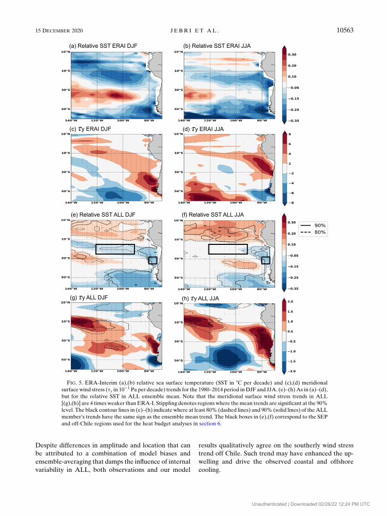
Despite differences in amplitude and location that can

be attributed to a combination of model biases and

ensemble-averaging that damps the influence of internal

variability in ALL, both observations and our model

results qualitatively agree on the southerly wind stress

trend off Chile. Such trend may have enhanced the up-

welling and drive the observed coastal and offshore

cooling.

FIG. 5. ERA-Interim (a),(b) relative sea surface temperature (SST in 8C per decade) and (c),(d) meridional

surfacewind stress (ty in 1021 Pa per decade) trends for the 1980–2014 period inDJF and JJA. (e)–(h)As in (a)–(d),

but for the relative SST in ALL ensemble mean. Note that the meridional surface wind stress trends in ALL

[(g),(h)] are 4 times weaker thanERA-I. Stippling denotes regions where themean trends are significant at the 90%

level. The black contour lines in (e)–(h) indicate where at least 80% (dashed lines) and 90% (solid lines) of theALL

member’s trends have the same sign as the ensemble mean trend. The black boxes in (e),(f) correspond to the SEP

and off-Chile regions used for the heat budget analyses in section 6.

15 DECEMBER 2020 J EBR I ET AL . 10563

Unauthenticated | Downloaded 02/26/22 12:24 PM UTC

Figure 6 displays the time evolution of variables that

characterize the variations of the upwelling off central

Chile. The dynamical variables have physically con-

sistent variations during both seasons, with southerly

(positive) wind stress, negative wind stress curl, and

positive ocean velocities all consistent with an en-

hanced wind-driven upwelling (Figs. 6b,d). In DJF,

these variables start evolving around the mid-1970s to

reach a new steady state with higher mean values

around 2000 (Fig. 6b). While those dynamical param-

eters clearly point to an increased upwelling in re-

sponse to the external forcing, the picture is less clear

for SST that remains relatively steady in the 1980s but

then warms from the mid-1990s onward. This may be

due to the compensation between the cooling driven

by the enhanced upwelling of cold subsurface water

and warming due to positive radiative forcing. In austral

winter (JJA), the upwelling enhances more clearly from

the late 1990s onward, when SST has already started

rising due to the radiative forcing (Fig. 6d). It is also

reasonable to hypothesize that cooling due to the in-

crease of the upwelling is partly counterbalancing the

radiatively forced SST increase during this season as

well.Wewill investigate this hypothesis in more detail in

section 6.

b. Relative roles of forced versus internal variabilityon simulated regional trends

In this subsection, we characterize the relative con-

tributions of externally forced and internal variability

on decadal and multidecadal variations in the Pacific in

our model. In ALL we rely on an empirical orthogonal

function (EOF) analysis of SST, sea surface height (SSH),

and zonal (tx) and meridional (ty) wind stress in the

Pacific sector between 608N and 508S (Fig. 7). Figure 7a

displays the PC time series obtained from projecting

FIG. 6. Area averagedmeridional surfacewind stress (ty, blue, in 1022Nm22), sea surface temperature (SST, red, in 8C),

wind curl (§, green, in 1029Nm23), and vertical velocity at 100-m depth in the ocean (W100, purple, in mday21) for ALL

in (b) DJF and (d) JJA. Thick solid lines indicate the ensemble means; shading shows the 95% confidence interval. The

regions used for the area average are shown in (a),(c), colored, respectively, as the variables (see section 2c).

10564 JOURNAL OF CL IMATE VOLUME 33

Unauthenticated | Downloaded 02/26/22 12:24 PM UTC

each ensemble member on the first EOF of ALL en-

semble mean (Fig. 7b; hereafter EOF-FOR), that is, a

robust estimate of the model externally forced re-

sponse. EOF-FOR explains 98%, 78%, 88%, and 98%

of the total variance of the ensemble-mean SST, ty, tx,

and SSH, respectively (Fig. 7a; the ensemble mean and

spread are displayed).We then isolated the leading mode

of internal variability (EOF-IPO) by applying an EOF

analysis of ALL individual members residuals, after

removing signals associated with EOF-FOR (Figs. 7c,d).

The first PCs fromEOF-IPO (Fig. 7c) explain 29% of the

ensemble total variance for SST and ty, 26% for SSH, and

22% for tx, respectively. The related PCs exhibit a much

larger spread than the first EOF-FOR PCs, as expected

from internally generated climate variability. Their spatial

pattern (Fig. 7d) strongly projects onto that of the IPO, the

leading mode of observed internal variability at decadal

time scale (Deser et al. 2010). This procedure is used to

FIG. 7. EOFs and associated standardized PCs for ALL sea surface temperature (SST, in blue), meridional

surface wind stress (ty, red), zonal surface wind stress (tx in green), and sea surface height (SSH in purple) derived

from (a),(b) the leading ensemble mean EOF for each variable (EOF-FOR, capturing 80%–98% of the ensemble

mean variations) and from (c),(d) the leading EOF of the residual (EOF-IPO) obtained after removal of the forced

components. Shading in (a) and (c) shows the 90% confidence interval. (b) The regression pattern for the EOF-

FOR and (d) the EOF-IPO PCs for each variable on the corresponding field anomalies of SST (color shading,

in 8C), surface wind stress (arrows, in 0.1 Pa), and SSH (in m; contours). The percentage of variance explained by

the reconstructed ty (shading) and SST (white contours) field using the corresponding EOF-FOR and EOF-IPO

PCs for the 1980–2014 period are shown in (e) and (f), respectively. The white and black contours in (b) and (d) for

SSH, are in meters per standard deviation. The black boxes in (e),(f) correspond to the SEP and off-Chile regions

used for the heat budget analyses in section 6.

15 DECEMBER 2020 J EBR I ET AL . 10565

Unauthenticated | Downloaded 02/26/22 12:24 PM UTC

separate the forced signal (EOF-FOR) from the leading

mode of internal variability at decadal scale (EOF-IPO).

The forced surface wind stress, SST and SSH evolu-

tions obtained from EOF-FOR (Figs. 7a,b) are consis-

tent with Fig. 1d, and display enhanced trade winds over

the central equatorial Pacific. Ourmodel results contrast

with the majority of CMIP3/5 scenario simulations that

rather project a weakened Walker circulation and an El

Niño–like response pattern, with the central and eastern

equatorial Pacific SST warming more than the western

equatorial Pacific in response to anthropogenic climate

change (e.g., Collins et al. 2005; Held and Soden 2006;

Kociuba and Power 2015). The SSH also rises more in

the western Pacific in our model, in response to the

strengthened equatorial trades.

In our region of focus, EOF-FOR reveals a weaker SST

warming than in other regions and a wind strengthening

in an oblique band from the Chilean coast to the central

equatorial Pacific (Fig. 7b). In ALL, the forced compo-

nent of the simulated variability accounts for more than

60% of the upwelling-favorable meridional wind stress

(ty) increase (Fig. 7e) and about 20% of SST decadal

variability locally off Chile (white contours in Fig. 7e). In

contrast, internal variability related to IPO has no sig-

nificant contribution to meridional wind stress and SST

variability off Chile (Fig. 7f), but mostly contributes to

these variables in the North Pacific. Farther offshore in

the SEP box, the SST internal decadal variability is more

important (Fig. 7f), the IPO explaining 10%–20% of SST

variance while the forced component accounts for more

than 40% (Fig. 7e). This analysis hence indicates that

in our model IPO-related SST changes are weak relative

to the forced changes in the SEP region, and very weak in

the Chile upwelling region.

c. Relative roles of forced versus internal variabilityon observed regional trends

To evaluate the robustness of our model results and

provide an estimate of the relative roles of external

forcing and the IPO in observations, Figs. 8a–c display

the regressed SST, surface winds, and sea level pressure

(SLP) fields onto indices of the global warming signal

(globally averaged SST) and IPO for the 1940–2014

period. The results reveal the imprint of the radiatively

induced global warming except in North Pacific, south-

ern Pacific, and off the Chilean coast where there is no

warming signal. The global mean SST explains 1%,

32%, and 53% of the total variance for SST, meridional

winds, and SLP, respectively, off Chile while the IPO

explains 23% of SST variance and 1% of variance on

average for both meridional winds and SLP variables

(Figs. 8d–g). Farther offshore in the SEP region, the SST

internal decadal variability related to IPO explains 37%,

30%, and 37% of SST, meridional winds and SLP vari-

ance, respectively, while the forced component accounts

for 19%, 5%, and 17%. This analysis hence suggests that

IPO-related upwelling-favorable meridional winds and

related SLP changes in the Chile upwelling region are

not significant, the coastal region being dominated by the

forced changes while farther offshore in the SEP box, the

SST internal decadal variability plays a more important

role. These results are robust when the analysis is per-

formed over a shorter, better-observed period (1960–2014;

not shown). This analysis supports our conclusions based

on our model large ensemble that the relative cooling

off Chile and in the SEP might be tightly linked to the

anthropogenic external forcing signal, which probably

exerts a dominant role in reinforcing the coastal upwelling.

To further evaluate the role of the IPO phase on 1980–

2014 regional SST trends in our model and observations,

we show relative SST (RSST) trends in the SEP and off-

Chile regions separately for ensemble members with a

positive or negative IPO trend during the period (about

half of the members for each, Fig. 9a). In observations, the

negative IPO trend (20.298Cdecade21; green vertical

dashed line in Fig. 9a) is associated with a significant rel-

ative cooling trend both off Chile (20.178Cdecade21) and

in the SEP box (20.148Cdecade21) regions (Figs. 9b,c;

green vertical dashed line). In the model, however, the

phase of the IPO does not have a clear fingerprint on local

nor regional RSST trend. A significant RSST decrease off

Chile (20.208Cdecade21) and in SEP (20.128Cdecade21)

is simulated and its amplitude is consistent with observa-

tions, regardless of the IPO phase. This suggests again that

the internally generated SST decadal variability is over-

whelmed by the external forcing influence in ALL during

the period 1980–2014. External forcing therefore likely

influences the observed 1980–2014 trend.

Overall, this section demonstrates that the strength-

ening of the southerlies over recent decades is domi-

nated by external forcing, both at the coast and offshore.

The relative cooling trend is also dominated by external

forcing in the Chile upwelling and SEP regions, with a

larger contribution of internal variability (including the

IPO) in the SEP. In the following section, we will relate

this southerly wind anomaly to theHadley cell extension

and attribute this extension to specific external forcing.

5. Influence of the HC meridional extension andattribution to individual forcing

a. Connections between the HC and the PCUS

The strengthening of upwelling-favorable winds off

Chile can be explained by large-scale atmospheric circu-

lation changes. The climatological low-level atmospheric

circulation in the PCUS region is associated with the

10566 JOURNAL OF CL IMATE VOLUME 33

Unauthenticated | Downloaded 02/26/22 12:24 PM UTC

eastern flank of the South Pacific anticyclone (SPA;

Figs. 10a,b, black contours). We now evaluate the fol-

lowing hypotheses for explaining the development of

externally forced southerly anomalies in the PCUS

region: either a southward expansion of the HC and

southward shift of the SPA (e.g., Belmadani et al. 2014) or

strengthening of the land-ocean sea level pressure contrast

in the context of climate change (Bakun et al. 2010).

FIG. 8. (a) IPO (black curve; tripole index see section 2d), global warming signal (blue curve; globally averaged SST),

atmospheric GHG (red curve; as provided by CMIP6), and stratospheric ozone (green curve; as provided by CMIP6)

standardized indices for the 1940–2014 period. (b) The regression pattern on the IPO and (c) the global mean SST

standardized indices on field anomalies of SST (ERSSTv4 dataset; color shading, in 8C), 10-m winds (fromNOAA-20C

reanalyses; vectors, inm s21), and sea level pressure (SLP, fromNOAA-20C reanalyses; contours, in Pa). The percentage

of variance explained for themeridional 10-mwind (color shading), SST (white contours), and SLP (color shading) field

using the IPO and global mean SST indices are shown in (d),(f) and (e),(g), respectively. The black contours in (b) and

(c) for SLP are in Pa per standard deviation. The black boxes in (d)–(g) locate the SEP and off-Chile regions.

15 DECEMBER 2020 J EBR I ET AL . 10567

Unauthenticated | Downloaded 02/26/22 12:24 PM UTC

We isolate regions of homogeneous variability of

meridional wind stress and vertical velocity at 100-m

depth off Chile to build area-average low-pass-filtered

time series for both variables (colored contours in

Figs. 10a and 10b; see section 2d). Figures 10a and 10b

display the regression of the SLP anomalies onto the

low-pass-filtered meridional wind stress time series off

Chile in ALL (Figs. 10a,b). Southerly wind anomalies

off Chile since the 1970s (1990s) in DJF (JJA) are as-

sociated with positive SLP anomalies in the southern

edge of the SPA, consistent with the HC poleward ex-

pansion in other CMIP5models (e.g., Min and Son 2013;

Choi et al. 2014; Nguyen et al. 2015). TheALL ensemble

mean, however, does not reproduce a decline of SLP

inland over South America, as would be expected from

the Bakun et al. (2010) mechanism.

To further illustrate the relationship between the

Southern Hemisphere HC edge (see section 3d) and the

SPA, we define an area-averaged low-pass-filtered SLP

index, using box average over the region outlined on

Figs. 10a and 10b (yellow box). The high correlation

(0.98 and 0.96 in DJF and JJA, respectively) between

the latitudinal position of the southern edge of the HC

(as defined in section 3d) and the SPA SLP further il-

lustrates the strong link between the HC southward

expansion and SPA strengthening (Fig. 10c). We also

find strong relations between the SPA SLP and the low-

pass-filtered time series of the velocity at 100-m depth

(upwelling intensity) off Chile (correlation values of

0.97 and 0.98 in DJF and JJA, respectively, Fig. 10d).

Overall, analyses in this subsection illustrate a strong

link between the simulated positions of theHC southern

boundary, the intensification of the SPA, the southerly

winds, and the strengthened coastal upwelling off the

Chilean coast.

b. Attribution of HC variations to individual externalforcing

Figure 11 displays the time series of the ensemble-

mean latitude of the Southern Hemisphere HC pole-

ward edge inALL,GHG, andOZ during 1940–2020 and

in twentieth-century NOAA–CIRES (Compo et al.

2011), NCEP (Kalnay et al. 1996), andERA-I (Dee et al.

2011) reanalyses. The reanalyses and ALL ensemble

mean all reveal (with the exception of NCEP in JJA) a

significant poleward shift of the subsiding branch of the

Hadley cell, from the 1970s onward with a stabilization

during the last two decades of the simulated period. The

shift is more pronounced in DJF (;0.88S in 1980–2014)

than in JJA (;0.458S). ALL results are within the range

of reanalyses uncertainties, which indicate a 0.258 to 38poleward expansion of the HC southern edge since the

seventies (Figs. 11c,d; Seidel and Randel 2007; Staten

et al. 2018; Grise et al. 2019).

Single-forcing experiments suggests that volcanic forc-

ing does not contribute to the HC southward expansion

(Figs. 11a,b). During austral winter (JJA), the ozone con-

tribution is also weak, and the greenhouse gas forc-

ing dominates the HC expansion, producing a linear

trend in the HC poleward expansion, from 1970 to 2020

(Fig. 11b). GHG and stratospheric ozone depletion

both act to expand theHC in austral summer, the impact

of ozone depletion dominating before 1995 in agree-

ment with previous studies (e.g., Min and Son 2013;

FIG. 9. Probability density function (pdf) for (a) the IPO index trends during 1980–2014 (8Cdecade21). We computed the IPO index

[relying on the tripole index (TPI) from Henley et al. (2015)], defined as the central equatorial Pacific SST (108S–108N, 1708E2908W)

minus the average of northwest (258–458N, 1408E21458W) and southwest (158–508S, 1508E21608W) Pacific SST, smoothed using a 13-yr

Chebyshev low-pass filter (see section 2d). We then use this index to build a pdf of 34-yr-long IPO index trends allowing to split between

positive (red bars) and negative (blue bars) trends. (b) As in (a), but for the relative sea surface temperature (RSST) trends (in

8Cdecade21) off Chile. (c) As in (b), but in SEP. The off-Chile and SEP regions used for the SST area-averaged in (b) and (c) are shown as

black rectangles in Figs. 5 and 7. The vertical dashed lines in (a)–(c) correspond to ALL ensemble mean (black) and the mean for positive

(red bars) and negative (blue bars) IPO index trends. The green vertical dashed lines correspond to ERSSTv4 trends. Note we use relative

SST anomalies, respectively, to the global mean SST for both ERSSTv4 and ALL (see text).

10568 JOURNAL OF CL IMATE VOLUME 33

Unauthenticated | Downloaded 02/26/22 12:24 PM UTC

Waugh et al. 2015). After 1995, the ozone recovery

(Szopa et al. 2013) yields a stabilization of the ozone

contribution to the HC expansion, at a level similar to

that of GHGs. Together, these two effects yield an

austral summer HC meridional expansion from 1970 to

2000, followed by stabilization from 2000 onward.

c. Attribution of PCUS variations to various externalforcing

Since all the variables that characterize the PCUS are

highly correlated (see section 4a), Fig. 12 displays only

SST and w100 (hereafter upwelling) anomalies in single-

forcing ensemble simulations. The (GHG 1 VOLC 1OZ)mean SST andw100 time series fit well with theALL

curve, suggesting a linear additivity of each individual

externals forcings. Increased upwelling caused by the

ozone depletion (Fig. 12a) explains most of the SST

cooling visible in the early 1980s in DJF (Fig. 12c). The

SST variations in OZ hence largely reflect wind-driven

changes linked to stratospheric ozone changes. These

effects of the ozone forcing start decreasing after 1995 in

association with the ozone recovery. GHG contributes

FIG. 10. Sea level pressure (SLP) 1941–61 climatology (black contours, every 4 hPa) and linear regression

(shading, in hPa Pa21) of the SLP on the mean meridional surface wind stress off Chile in (a) DJF and (b) JJA for

the 1980–2014 period using ALL Ensemble mean. (c) Scatterplot between the latitudinal positions of the Southern

HemisphereHadley cell boundaries vs the area averaged South Pacific sea level pressure (SLP, in hPa) anomalies in

DJF (DJFs, crosses) and JJA (JJAs, dots). (d) Scatterplot between vertical velocity at 100-m depth (W100, in

m day21) off the Chilean coast with the area averaged South Pacific SLP anomalies (in hPa) in DJF (crosses) and

JJA (dots). The scatterplots are using values from ALL ensemble mean. The coefficient of determination (R2)

between each variable is given in (c),(d). The dots and crosses in (c),(d) are colored from the oldest (dark blue) to

the most recent years (yellow) of the simulation for the whole 1940–2020 period. The blue and red lines show the

regression lines in DJF (blue) and JJA (red). The yellow box in (a),(b) corresponds to the regions used for the SLP

South Pacific anticyclone. The blue and purple contours in (a),(b) indicate the region used for the area average of

meridional surface wind and W100 off Chile.

15 DECEMBER 2020 J EBR I ET AL . 10569

Unauthenticated | Downloaded 02/26/22 12:24 PM UTC

mainly to upwelling changes in JJA (Fig. 12b) through

dynamically induced cooling but this is overwhelmed by

radiatively induced warming (Fig. 12d). Hence the two

competing effects between cooling through strength-

ened upwelling and warming through GHGs, radiative

effect sustain the relatively limited surface warming off

Chile as compared to the surrounding regions (Fig. 1).

Even if the volcanic forcing contributes through a small

weakening after Agung (March 1963), El Chichón (April

1982), and Pinatubo (June 1991), we clearly see a dy-

namical response with an upwelling intensification in re-

sponse to the anthropogenic forcing during both seasons.

GHG and OZ forcing within ALL combine to produce

the upwelling intensification since the 1970s. This up-

welling intensification first counteracts the effect of the

GHGs radiative forcing, leading to a stable SST until

;2000.After the ozone recovery, the forcing fromGHGs

overwhelms the cooling effect of the enhanced upwelling,

yielding a SST increase. Overall, this is consistent with

the weaker SST increase off Chile than in surrounding

regions, in response to radiative forcing. In the follow-

ing section, we further investigate this surface warming

using a simplified heat budget of the upper oceanic layer.

6. Why does the southeast Pacific warm less thanthe rest of Pacific Ocean?

We contrast the SST upper ocean budget of our two

regions of interest, namely nearshore off Chile (328–308S,

808–758W) and farther offshore in the subtropical SEP

(258–178S, 1208–908W; Fig. 13a), with that of the entire

Pacific (508S–508N, 1208E–758W), in order to elucidate

why these two regions warm at a reduced rate. The

average Pacific warming starts 20 years earlier in the

1970s and is larger (11.28C in 2020) than that of the SEP

(10.68C) and off-Chile (10.28C) regions (Fig. 13b). Thecontributions from the surface heat flux (labeled ATM;

first term in the rhs of Eq. (1) in section 2d) and the

oceanic processes (labeled OCEdyn, second term in the

rhs of Eq. (1), including lateral and vertical advection

and mixing) are detailed in Fig. 13c.

At the scale of the PacificOcean (Fig. 13c, red curves),

the GHG forcing induces a positive net air–sea flux

(dominated by downward longwave radiation, not shown)

that warms the ocean, as expected from the effect of

greenhouse gases (e.g., Barnett et al. 2005). A cooling

by oceanic processes largely compensates this warm-

ing. The climate change induced warming indeed oc-

curs predominantly in the ocean surface layer (e.g.,

Barnett et al. 2005), and hence increases the tempera-

ture difference between the surface layer and the sub-

surface, and thus the cooling by turbulent fluxes at the

bottom of the mixed layer. In the nearshore region, the

warming is also due to atmospheric heat fluxes, but

partly compensated by a larger cooling due to increased

upwelling. This is supported by Fig. 13c (blue curves),

which reveals a stronger cooling by oceanic processes

in the off-Chile region (presumably largely because of

FIG. 11. Time series of the poleward edge of the Southern Hemisphere Hadley cell in (a) December–February

(DJFs) and (b) June–August (JJAs) for ALL (blue), GHG (orange), VOLC (green), and OZ (red). Colored thick

solid lines indicate the ensemble means, shading shows the 95% confidence interval. The sum between GHG,

VOLC, and OZ is shown as a black dashed curve. The vertical dashed lines indicate the timing of Agung (March

1963), El Chichón (April 1982), and Pinatubo (June 1991) eruptions. (c),(d) As in (a),(b), but for NCEP (in yellow),

NOAA-CIRES 20CR (in pink), and ERA-I (in black) reanalyses. Solid thick lines correspond to the annual time

series and dashed lines after applying a 7-yr Hanning filter.

10570 JOURNAL OF CL IMATE VOLUME 33

Unauthenticated | Downloaded 02/26/22 12:24 PM UTC

changes in upwelling) than over the entire Pacific (pre-

sumably largely because of changes in thermal stratifi-

cation and vertical mixing of heat). Figure 13f displays

upward velocity and cooling trends in the top 500m near

the coast off Chile that supports this view.

It is intriguing that in the offshore SEP region the

warming rate is also less than for the Pacific average

since it is not an upwelling region (Fig. 13b, green

curve). There, the impact of atmospheric net air–sea

heat fluxes trend [Qatm in Eq. (2)] is almost nearly

neutral (Fig. 13d, green dashed line) due to a balance

between increased longwave radiations [Qlw in Eq. (2)]

contributing to warming (6.288Cdecade21 during 1980–

2014) and the negative trend of net shortwave radiations at

ocean surface [Qsw 2 Qswh in Eq. (2); 24.258Cdecade21

during 1980–2014], assuming a fixed climatological mixed

layer depth. Indeed, more low-level clouds are increas-

ingly formed over the SEP region (not shown), due to

relatively colder SST and boundary layer stratification

under the synoptic HC descent over the SEP region

(Bony et al. 2006), which results in a local planetary al-

bedo increase. The strengthening of the surface wind

anomalies also favors cooling through enhanced latent

heat flux (24.038Cdecade21 during 1980–2014), while

sensible heat fluxes anomalies explain a small warming

(10.638Cdecade21 during 1980–2014). Near the coast,

however, low-level cloud cover decreases in response

to a stronger southerly coastal jet in our simulations.

This is consistent with the observed synoptic-scale co-

variability of surface winds and low cloud cover off Chile

at 338S (Garreaud and Muñoz 2005). Consequently, thedownward shortwave flux is more intense near the coast

than offshore, resulting in a larger Qatm. Wind stress

strengthening over SEP and coastal regions (Figs. 5g,h)

also influences the mixed layer depth and hence could

modulate the atmospheric heat fluxes impact on SST.

The respective roles of the mixed layer thickness (h)

and net surface downward heat flux (Q) variations in

ATM can be evaluated by fixing either h or Q to their

climatological values (Fig. 13d). Whereas SST increases

in the three considered regions, the mixed layer depth

increases during 1960–2000 particularly in DJF at rates

over 0.9 and 0.7mdecade21 in the SEP and nearshore

regions, respectively, whereas no changes is evidenced

on average over the Pacific basin (figures not shown).

The annual-mean surface net heat flux in the SEP region

being positive (4.80Wm22 in ALL), a thickening of

the mixed layer (and hence higher mixed layer heat

capacity) results in a decrease of heating rate by surface

heat fluxes (25.188Cdecade21 during 1980–2014; green

solid curve in Fig. 13c; green crossed line in Fig. 13d)

(i.e., an anomalous cooling).

FIG. 12. (a),(b) Off-Chile vertical velocity at 100-m depth (in m day21) and (c),(d) sea surface temperature

(in 8C) in DJF and JJA for ALL (blue), GHG (red), VOLC (green), and OZ (purple). The regions used for the

area average off Chile are shown as purple and red contours in (a) and (c) of Fig. 6. The sum between GHG,

VOLC, and OZ is shown as a black dashed curve and dashed–dotted lines. Colored thick solid lines indicate the

ensemble means; shading shows the 95% confidence interval.

15 DECEMBER 2020 J EBR I ET AL . 10571

Unauthenticated | Downloaded 02/26/22 12:24 PM UTC

In contrast, the ocean processes in the SEP con-

tribute to an anomalous warming trend (green dashed

curve in Fig. 13c). This can be explained neither by

changes in vertical velocities nor mixing, because these

changes (upwelling tendency and larger warming near

the surface, Fig. 13e) would rather be conducive to

cooling. This suggests that changes in lateral advection

drive the warming. The SEP reduced warming with

respect to its surroundings (Fig. 13a) implies a warm-

ing trend due to the advection of anomalous SST by

mean surface currents. The currents’ changes also in-

volve a southward component (due to Ekman transport,

FIG. 13. ALL (a) ensemble mean trends of sea surface temperature (SST, shading, 8Cdecade21) and surface current (arrows,

103m day21 decade21) over 1980–2014, (b) sea surface temperature anomalies, and (c) integrated net mixed layer heat budget for the

Pacific basin (red curves), southern Pacific (SEP, green curves), and off-Chile (blue curves) regions. The regions used for the SEP and off-

Chile area averages are shown as black boxes an (a). In (c) the thick solid lines correspond to the influence of heat flux (ATM) and the

dashed lines to the influence of oceanic processes (OCEdyn); see section 2e for details. (d) Influence of heat flux considering both heat flux

(Q) andmixed layer (h) variations (thick solid lines), onlyQ (dashed lines), or only h variations (crossed lines). The h0 andQ0 in the legend

indicate that the climatological value is used for the calculation. Thick lines indicate the ensemble means while shading shows the 90% con-

fidence interval. (e),(f) Vertical section of potential temperature (color shading, 8Cdecade21) and velocity (arrows, 102mday21 decade21)

trends over 1980–2014 period off Chile at 30.58S and in SEP region at 29.58S, respectively, for theALL ensemblemean.A scaling factor of 1.43104 off-Chile and 1.6 3 104 in SEP is applied on the vertical velocity.

10572 JOURNAL OF CL IMATE VOLUME 33

Unauthenticated | Downloaded 02/26/22 12:24 PM UTC

Fig. 13a) that increases the southward advection of

warmer water from farther north.

7. Discussion and conclusions

A SST cooling trend is observed off northern Chile

since 1980 and off southern Peru since themid-twentieth

century. Bakun et al. (2010) argue that surface pressure

decreases more on land than over the ocean in response to

anthropogenic forcing, giving rise to upwelling-favorable

winds in eastern boundary upwelling systems (EBUS),

which would explain the PCUS cooling trend. The ob-

served negative interdecadal Pacific oscillation (IPO)

trend over the same period is, however, also associated

with cooling in the southeastern Pacific and could con-

tribute to the observed trend. In this study, we quantify

the relative role of internal and external forcing in this

trend, and the associated mechanisms. Our ensemble-

mean historical simulation reproduces a weaker recent

SST trend in the southeastern part of the basin than

in the surroundings, with virtually no warming off Chile

since the 1970s, and a southerly wind anomaly at the

coast and offshore.

In line with other studies based on CMIP5 models

(e.g., Wang et al. 2015; Rykaczewski et al. 2015), we find

no clear low pressure trend over South America that

could lead to a southerly wind and upwelling intensifi-

cation. The externally forced component of the simulated

variability accounts for more than 60% of upwelling-

favorable meridional wind stress increase off Chile,

while a negative IPO canonical internal variability pat-

tern has no significant contribution to the meridional

wind stress positive trend over the same period. In the

real world the IPO has a different spatial structure,

amplitude and time behavior to that in CMIP5-class

models (Kravtsov 2017). Analyses of observed decadal

trends in SST, wind stresses and SLP separated into the

IPO and forced components are however consistent

with our model results. Hence, regional and local SST

cooling patterns in the SEP and off Chile might be

tightly linked to the anthropogenic external forcing

signal, which potentially exerts a dominant role in re-

inforcing the costal upwelling. PCUS can also be mod-

ulated by coastally trapped waves remotely forced by

equatorial Pacific zonal wind fluctuations (Montecinos

et al. 2007). This process may also contribute to the

coastal upwelling enhancement.

Previous modeling work shows that south of 338S the

poleward South Pacific anticyclone migration causes

geostrophy to break down due to the Andes orographic

barrier (Muñoz and Garreaud 2005; Belmadani et al.

2014), locally precluding the establishment of the geo-

strophic equilibrium in the alongshore direction. This

probably explains why the increase in modeled along-

shore winds is rather associated with an intensification

of the alongshore pressure gradient. We further link the

development of these southerly wind anomalies to a

poleward expansion of the Southern Hemisphere Hadley

cell, and strengthened South Pacific anticyclone, from

around 1980 until a new steady state is reached in austral

summer 2000 and in austral winter 2010. Attribution

analyses demonstrate that enhanced alongshore winds

and upwelling near the Chilean coast are due to

greenhouse gases and ozone anthropogenic forcings,

as both contribute to shift poleward the Hadley cell

southern boundary (e.g., Staten et al. 2018; Grise et al.

2019). The large tendency in the 1980s and the rela-

tively stable steady state later are consistent with the

reduced influence of stratospheric ozone after 1995.

The upwelling intensification is the main driver of the

negative relative SST (RSST) trend along the Chilean

coast. Farther offshore, previous studies suggest that the

mainmechanism for the robust negativeRSST trend in the

SEP region is thewind–evaporation–SST (WES) feedback

(e.g., Xie et al. 2010; Timmermann et al. 2010; Lu andZhao

2012) (i.e., that stronger winds enhance evaporative cool-

ing locally). Instead, we find a dominant role of the wind-

forced mixed layer deepening, which leads to a decreased

warming rate by surface air–sea fluxes.

A potential caveat of our study is the coarse spatial

resolutions of both the atmospheric (1.878 in latitude and

3.758 longitude) and ocean (28 horizontal resolution of

Chile) components of the IPSL-CM5A coupled model.

Our coarse model resolution (similar to CMIP5 class

models) does not resolve several small-scale coastal

processes, such as those associated with mesoscale oce-

anic eddies that contribute to the offshore transport of the

cold upwelled water (e.g., Colas et al. 2013), coastal capes

(e.g., Renault et al. 2016), sea breeze (Franchito et al.

1998), and the intensified temperature gradient induced

by the warming of the narrow plains between the coast

and the high Andes off Peru and northern Chile (e.g.,

Garreaud and Falvey 2009). Our results are nevertheless

consistent with those obtained by Belmadani et al. (2014)

that used an atmospheric model at higher horizontal res-

olution (50km). Relying on dynamical downscaling of

global GCM climate scenarios, Belmadani et al. (2014)

obtain a wind strengthening off central Chile around 308–358S and aweakening or no changes off Peru in agreement

with regional atmosphericmodeling (horizontal resolution

;45km)works byQuijano-Vargas (2011) andMuñoz andGarreaud (2005) for central Peru and north-central Chile

coastal regions, respectively. These studies did not how-

ever include coupling with the ocean. Future work with

regional coupled models at higher spatial resolution will

be needed to confirm the robustness of our results.

15 DECEMBER 2020 J EBR I ET AL . 10573

Unauthenticated | Downloaded 02/26/22 12:24 PM UTC

Themodel and observations are consistent in terms of

relative SST (i.e., in displaying a cooling relative to the

regional average in the SEP and PCUS). However, in

terms of absolute SST, the observations indicate a slight

cooling trend in the PCUS region, while the model

indicates a slight warming trend. This is most likely as-

sociated with the too strong climate sensitivity of our

climate model (Andrews et al. 2012; Forster et al. 2013),

which results in an overestimated surface global warming

that offsets the regional cooling trend. This is accentuated

by the fact that aerosol forcing (which induces a global

cooling trend) is omitted in our simulation. We however

probably partly remove this bias by using relative SST

(i.e., subtracting the overestimated global mean SST

warming). Our approach relying on relative SST, ob-

servations, and large ensembles needed to explore the

regional responses to internal variability and to forcing

histories nevertheless allows shedding light on the in-

trinsic dynamics of the southeast Pacific in recent de-

cades. Upcoming CMIP6 simulations would offer the

possibility to evaluate those results in a multimodel

context.

We did not discuss changes along the tropical Peruvian

coast (48–158S) in detail since this region does not display

any clear relative SST cooling or significant changes in

wind intensity in the ALL ensemble mean. Previous

studies however suggest that SST trends off northern

Peru are dominated by more frequent central Pacific El

Niños after 1980 (Dewitte et al. 2012). Note that the

analysis of observed winds also suggests no clear trend in

the northern part of the Peruvian upwelling (Belmadani

et al. 2014) despite the negative IPO trend during 1980–

2014 (Vuille et al. 2015). Other eastern boundary up-

welling systems (EBUS) of the Southern Hemisphere

such as the Benguela system off southern Africa (e.g.,

Lamont et al. 2018) and the one west of Australia (e.g.,

Rousseaux et al. 2012) do not appear to show any cooling

(Fig. 1). Observed SST trends during 1980–2014 in the

Atlantic Ocean mainly capture a large tropical Atlantic

warming (Li et al. 2016) while Indian Ocean SST

displays a warming trend that may reflect the global

warming signal (Dong and McPhaden 2016; Fig. 1).

Dedicated studies are needed to attribute the ocean

expression of the Southern Hemisphere HC expansion

in other southern EBUSs, which largely depends on the

local features such as bottom topography, mixed layer

depth, net surface fluxes, strength of the stratification,

and regional ocean currents.

To summarize, we find that GHG increase and ozone

depletion over the last few decades project onto robust

southeasterly wind stress and negative RSST trend pat-

terns in the southeastern Pacific. Anthropogenic forcings

dominate this negative RSST trend in our model, as

almost all the members display a weaker cooling in

the southeastern Pacific than in surrounding regions

(and the observed RSST trend lying within the simu-

lated distribution). Our results suggest that GHG and

ozone anthropogenic forcing are likely the key driving

factors for the recent observed PCUS intensification,

and that the recent negative IPO phase played little or

no role in this regional trend. Considering the continu-

ous increase in atmospheric GHG and the unexpected

and persistent global emissions of stratospheric ozone-

depleting CFC-11 since 2012 (Montzka et al. 2018), our

results provide practical guidance for the future climate

response in the PCUS.

Acknowledgments. This research was supported by the

French National Research Agency under the program

Facing Societal, Climate and Environmental Changes

(MORDICUS Project, Grant ANR-13-SENV-0002).

This work was granted access to the HPC resources of

TGCCunder the allocations 2016-017403 andA003017403

made by GENCI. This study also benefited from the IPSL

mesocenter facility, which is supported by CNRS, UPMC,

Labex L-IPSL (funded by the ANR Grant ANR-10-

LABX-0018 and by the European FP7 IS-ENES2 Grant

312979). We thank the ECMWF for providing the ERA-

Interim reanalysis. TheOISSTdatasetwas provided by the

NOAA/OAR/ESRL PSD, Boulder, Colorado. Support

for the Twentieth Century Reanalysis Project, version 2c,

dataset is provided by the U.S. Department of Energy,

Office of Science Biological and Environmental Research

(BER), and by the National Oceanic and Atmospheric

Administration Climate ProgramOffice. NCEP reanalysis

data are provided by the NOAA/OAR/ESRL PSD,

Boulder, Colorado (https://www.esrl.noaa.gov/psd/).

REFERENCES

Adam, O., T. Schneider, and N. Harnik, 2014: Role of changes in

mean temperatures versus temperature gradients in the recent

widening of the Hadley circulation. J. Climate, 27, 7450–7461,

https://doi.org/10.1175/JCLI-D-14-00140.1.

Alexander,M.A., I. Bladé, M. Newman, J. R. Lanzante, N.-C. Lau,

and J. D. Scott, 2002: The atmospheric bridge: The influence of

ENSO teleconnections on air–sea interaction over the global

oceans. J. Climate, 15, 2205–2231, https://doi.org/10.1175/1520-

0442(2002)015,2205:TABTIO.2.0.CO;2.

Allen, R. J., and O. Ajoku, 2016: Future aerosol reductions and

widening of the northern tropical belt. J. Geophys. Res. Atmos.,

121, 6765–6786, https://doi.org/10.1002/2016JD024803.

Andrews, T., J. M. Gregory, M. J. Webb, and K. E. Taylor, 2012:

Forcing, feedbacks and climate sensitivity in CMIP5 coupled

atmosphere-ocean climate models. Geophys. Res. Lett., 39,

L09712, https://doi.org/10.1029/2012GL051607.

Arakelian, A., and F. Codron, 2012: Southern Hemisphere jet

variability in the IPSL GCM at varying resolutions. J. Atmos.

Sci., 69, 3788–3799, https://doi.org/10.1175/JAS-D-12-0119.1.

10574 JOURNAL OF CL IMATE VOLUME 33

Unauthenticated | Downloaded 02/26/22 12:24 PM UTC

Aravena, G., B. Broitman, and N. C. Stenseth, 2014: Twelve years

of change in coastal upwelling along the central-northern

coast of Chile: Spatially heterogeneous responses to climatic

variability. PLOS ONE, 9, e90276, https://doi.org/10.1371/

journal.pone.0090276.

Bakun,A.,D. B. Field,A.Redondo-Rodriguez, and S. J.Weeks, 2010:

Greenhouse gas, upwelling-favorable winds, and the future of

coastal ocean upwelling ecosystems. Global Change Biol., 16,

1213–1228, https://doi.org/10.1111/j.1365-2486.2009.02094.x.

Balmaseda, M. A., K. E. Trenberth, and E. Källén, 2013: Distinctive

climate signals in reanalysis of global ocean heat content.Geophys.

Res. Lett., 40, 1754–1759, https://doi.org/10.1002/grl.50382.Barnes, E. A., and L. Polvani, 2013: Response of the midlatitude

jets, and of their variability, to increased greenhouse gases in

the CMIP5 models. J. Climate, 26, 7117–7135, https://doi.org/

10.1175/JCLI-D-12-00536.1.

Barnett, T. P., D. W. Pierce, K. M. AchutaRao, P. J. Gleckler, B. D.

Santer, J. M. Gregory, andW.M.Washington, 2005: Penetration

of human-induced warming into the world’s oceans. Science, 309,

284–287, https://doi.org/10.1126/science.1112418.

Bayr, T., and D. Dommenget, 2013: The tropospheric land–sea

warming contrast as the driver of tropical sea level pressure

changes. J. Climate, 26, 1387–1402, https://doi.org/10.1175/

JCLI-D-11-00731.1.

Beaugrand, G., and Coauthors, 2019: Prediction of unprecedented

biological shifts in the global ocean. Nat. Climate Change, 9,

237–243, https://doi.org/10.1038/s41558-019-0420-1.

Bellenger, H.,É. Guilyardi, J. Leloup,M. Lengaigne, and J. Vialard,

2014: ENSO representation in climate models: From CMIP3 to

CMIP5. Climate Dyn., 42, 1999–2018, https://doi.org/10.1007/

s00382-013-1783-z.

Belmadani, A., V. Echevin, F. Codron, K. Takahashi, and

C. Junquas, 2014: What dynamics drive future wind scenarios

for coastal upwelling off Peru and Chile? Climate Dyn., 43,

1893–1914, https://doi.org/10.1007/s00382-013-2015-2.

Boer, G., G. Flato, and D. Ramsden, 2000: A transient climate

change simulation with greenhouse gas and aerosol forcing:

Projected climate to the twenty-first century.ClimateDyn., 16,

427–450, https://doi.org/10.1007/s003820050338.

Bony, S., and Coauthors, 2006: How well do we understand and

evaluate climate change feedback processes? J. Climate, 19,

3445–3482, https://doi.org/10.1175/JCLI3819.1.

Bopp,L., andCoauthors, 2013:Multiple stressors of ocean ecosystems in

the 21st century: Projections with CMIP5 models. Biogeosciences,

10, 6225–6245, https://doi.org/10.5194/bg-10-6225-2013.

Brient, F., and S. Bony, 2013: Interpretation of the positive low-

cloud feedback predicted by a climate model under global

warming.ClimateDyn., 40, 2415–2431, https://doi.org/10.1007/

s00382-011-1279-7.

Capet, X. J., P. Marchesiello, and J. C. McWilliams, 2004:

Upwelling response to coastal wind profiles. Geophys. Res.

Lett., 31, L13311, https://doi.org/10.1029/2004GL020123.

Carton, J. A., andB. S.Giese, 2008:A reanalysis of ocean climate using

Simple Ocean Data Assimilation (SODA).Mon. Wea. Rev., 136,

2999–3017, https://doi.org/10.1175/2007MWR1978.1.

Chavez, F. P.,A.Bertrand,R.Guevara-Carrasco, P. Soler, and J.Csirke,

2008: The northern Humboldt Current system: Brief history,

present status and a view towards the future. Prog. Oceanogr., 79,

95–105, https://doi.org/10.1016/j.pocean.2008.10.012.

Chen, S., K. Wei, W. Chen, and L. Song, 2014: Regional changes

in the annual mean Hadley circulation in recent decades.

J. Geophys. Res. Atmos., 119, 7815–7832, https://doi.org/

10.1002/2014JD021540.

Choi, J., S. W. Son, J. Lu, and S. K. Min, 2014: Further observa-

tional evidence of Hadley cell widening in the Southern

Hemisphere. Geophys. Res. Lett., 41, 2590–2597, https://

doi.org/10.1002/2014GL059426.

Choi, J.-W., I.-G. Kim, J.-Y. Kim, and C.-H. Park, 2016: The recent

strengthening of Walker circulation. SOLA, 12, 96–99, https://

doi.org/10.2151/SOLA.2016-022.

Colas, F., X. Capet, J. C. McWilliams, and Z. Li, 2013: Mesoscale

eddy buoyancy flux and eddy-induced circulation in eastern

boundary currents. J. Phys. Oceanogr., 43, 1073–1095, https://

doi.org/10.1175/JPO-D-11-0241.1.

Collins, M., and Coauthors, 2005: El Niño- or La Niña-like climate

change? Climate Dyn., 24, 89–104, https://doi.org/10.1007/

s00382-004-0478-x.

Compo, G. P., and Coauthors, 2011: The Twentieth Century

Reanalysis project. Quart. J. Roy. Meteor. Soc., 137, 1–28,

https://doi.org/10.1002/qj.776.

Cushing, D. H., 1971: Upwelling and the production of fish. Adv.

Mar. Biol., 9, 255–334, https://doi.org/10.1016/S0065-2881(08)

60344-2.

de Boisséson, E., M. A. Balmaseda, S. Abdalla, E. Källeìn, andP. E. M. Janssen, 2014: How robust is the recent strengthening

of the tropical Pacific trade winds? Geophys. Res. Lett., 41,

4398–4405, https://doi.org/10.1002/2014GL060257.

Dee, D. P., and Coauthors, 2011: The ERA-Interim reanalysis:

Configuration and performance of the data assimilation sys-

tem.Quart. J. Roy. Meteor. Soc., 137, 553–597, https://doi.org/

10.1002/qj.828.

Deser, C., A. S. Phillips, and J. W. Hurrell, 2004: Pacific inter-

decadal climate variability: Linkages between the tropics

and the North Pacific during boreal winter since 1900.

J. Climate, 17, 3109–3124, https://doi.org/10.1175/1520-0442(2004)

017,3109:PICVLB.2.0.CO;2.

——, M. A. Alexander, S.-P. Xie, and A. S. Phillips, 2010: Sea

surface temperature variability: Patterns and mechanisms.

Annu. Rev. Mar. Sci., 2, 115–143, https://doi.org/10.1146/

annurev-marine-120408-151453.

Dewitte, B., and Coauthors, 2012: Change in El Niño flavours over

1958–2008: Implications for the long-term trend of the up-

welling off Peru. Deep-Sea Res. II, 77–80, 143–156, https://

doi.org/10.1016/j.dsr2.2012.04.011.

Dommenget, D., 2009: The ocean’s role in continental climate

variability and change. J. Climate, 22, 4939–4952, https://

doi.org/10.1175/2009JCLI2778.1.

Dong, L., and M. J. McPhaden, 2016: Interhemispheric SST gra-

dient trends in the IndianOcean prior to and during the recent

global warming hiatus. J. Climate, 29, 9077–9095, https://

doi.org/10.1175/JCLI-D-16-0130.1.

Dufresne, J.-L., and Coauthors, 2013: Climate change projections

using the IPSL-CM5 Earth system model: From CMIP3 to

CMIP5. Climate Dyn., 40, 2123–2165, https://doi.org/10.1007/

s00382-012-1636-1.

England, M. H., and Coauthors, 2014: Recent intensification of

wind-driven circulation in the Pacific and the ongoing warm-

ing hiatus. Nat. Climate Change, 4, 222–227, https://doi.org/

10.1038/nclimate2106.

Falvey, M., and R. D. Garreaud, 2009: Regional cooling in a

warming world: Recent temperature trends in the southeast

Pacific and along the west coast of subtropical South America

(1979–2006). J. Geophys. Res., 114, D04102, https://doi.org/

10.1029/2008JD010519.

Fichefet, T., and M. Maqueda, 1997: Sensitivity of a global sea ice

model to the treatment of ice thermodynamics and dynamics.

15 DECEMBER 2020 J EBR I ET AL . 10575

Unauthenticated | Downloaded 02/26/22 12:24 PM UTC

J. Geophys. Res., 102, 12 609–12 646, https://doi.org/10.1029/

97JC00480.

Fleming, L. E., and K. J. Anchukaitis, 2016: North Pacific decadal

variability in the CMIP5 last millennium simulations. Climate

Dyn., 47, 3783–3801, https://doi.org/10.1007/s00382-016-3041-7.

Folland,C.,D. Parker,A.Colman, andR.Washington, 1999: Large scale

modes of ocean surface temperature since the late nineteenth cen-

tury.BeyondElNiño:Decadal and Interdecadal ClimateVariability,

A. Navarra, Ed., Springer Science & Business Media, 73–102.

Forster, P. M., T. Andrews, P. Good, J. M. Gregory, L. S. Jackson,

and M. Zelinka, 2013: Evaluating adjusted forcing and model

spread for historical and future scenarios in the CMIP5 gen-

eration of climate models. J. Geophys. Res. Atmos., 118, 1139–

1150, https://doi.org/10.1002/JGRD.50174.

Foster, G., and S. Rahmstorf, 2011: Global temperature evolution

1979–2010. Environ. Res. Lett., 6, 044022, https://doi.org/

10.1088/1748-9326/6/4/044022

Franchito, S. H., V. B. Rao, J. L. Stech, and J. A. Lorenzzetti, 1998:

The effect of coastal upwelling on the sea-breeze circulation at

Cabo Frio, Brazil: A numerical experiment. Ann. Geophys.,

16, 866–871, https://doi.org/10.1007/S00585-998-0866-3.

Fréon, P., M. Barange, and J. Aristegui, 2009: Eastern boundary

upwelling ecosystems: Integrative and comparative ap-

proaches. Prog. Oceanogr., 83, 1–14, https://doi.org/10.1016/

j.pocean.2009.08.001.

Garreaud, R., and R. Muñoz, 2005: The low-level jet off the west

coast of South America: Structure and variability. Mon. Wea.

Rev., 133, 2246–2261, https://doi.org/10.1175/MWR2972.1.

——, and M. Falvey, 2009: The coastal winds off western sub-

tropical South America in future climate scenarios. Int.

J. Climatol., 29, 543–554, https://doi.org/10.1002/joc.1716.Gastineau, G., H. Le Treut, and L. Li, 2008: Hadley circulation

changes under global warming conditions indicated by cou-

pled climate models. Tellus, 60A, 863–884, https://doi.org/

10.1111/j.1600-0870.2008.00344.x.

——, A. Friedman, M. Khodri, and J. Vialard, 2018: Global ocean

heat content redistribution during the 1998-2012 Interdecadal

Pacific Oscillation negative phase. Climate Dyn., 53, 1187–

1208, https://doi.org/10.1007/S00382-018-4387-9%20.

Grise, K. M., and Coauthors, 2019: Recent tropical expansion:

Natural variability or forced response? J. Climate, 32, 1551–

1571, https://doi.org/10.1175/JCLI-D-18-0444.1.

Gutiérrez, D., and Coauthors, 2011: Coastal cooling and in-

creased productivity in the main upwelling zone off Peru

since the mid-twentieth century. Geophys. Res. Lett., 38,

L07603, https://doi.org/10.1029/2010GL046324.

Held, I. M., and B. J. Soden, 2006: Robust responses of the hy-

drological cycle to global warming. J. Climate, 19, 5686–5699,

https://doi.org/10.1175/JCLI3990.1.

Henley, B. J., J. Gergis, D. J. Karoly, S. Power, J. Kennedy, and

C. K. Folland, 2015: A tripole index for the Interdecadal

Pacific Oscillation. Climate Dyn., 45, 3077–3090, https://

doi.org/10.1007/s00382-015-2525-1.

Hourdin, F., and Coauthors, 2013: Impact of the LMDZ atmo-

spheric grid configuration on the climate and sensitivity of the

IPSL-CM5A coupled model. Climate Dyn., 40, 2167–2192,

https://doi.org/10.1007/s00382-012-1411-3.

Hu, Y., C. Zhou, and J. Liu, 2011: Observational evidence for

poleward expansion of the Hadley circulation. Adv. Atmos.

Sci., 28, 33–44, https://doi.org/10.1007/s00376-010-0032-1.

——, L. Tao, and J. Liu, 2013: Poleward expansion of the Hadley

circulation in CMIP5 simulations. Adv. Atmos. Sci., 30, 790–

795, https://doi.org/10.1007/s00376-012-2187-4.

Huang, B., and Coauthors, 2015: Extended Reconstructed Sea

Surface Temperature version 4 (ERSST.v4). Part I: Upgrades

and intercomparisons. J. Climate, 28, 911–930, https://doi.org/

10.1175/JCLI-D-14-00006.1.

Ibarra, A. A., C. Reid, andA. Thorpe, 2000: The political economy

of marine fisheries development in Peru, Chile and Mexico.

J. Latin Amer. Stud., 32, 503–527, https://doi.org/10.1017/

S0022216X00005824.

Johanson, C. M., and Q. Fu, 2009: Hadley cell widening: Model

simulations versus observations. J. Climate, 22, 2713–2725,

https://doi.org/10.1175/2008JCLI2620.1.

Joshi,M.M., J.M.Gregory,M. J.Webb,D.M.H. Sexton, and T. C.

Johns, 2008: Mechanisms for the land/sea warming contrast

exhibited by simulations of climate change. Climate Dyn., 30,

455–465, https://doi.org/10.1007/s00382-007-0306-1.

Kalnay, E., and Coauthors, 1996: The NCEP/NCAR 40-Year

Reanalysis Project. Bull. Amer. Meteor. Soc., 77, 437–471,

https://doi.org/10.1175/1520-0477(1996)077,0437:TNYRP.2.0.CO;2.

Kämpf, J., and P. Chapman, Eds., 2016: The Peruvian-Chilean

coastal upwelling system. Upwelling Systems of the World,

Springer, 161–194.

Kim, Y. H., S. K. Min, S. W. Son, and J. Choi, 2017: Attribution of

the local Hadley cell widening in the Southern Hemisphere.

Geophys. Res. Lett., 44, 1015–1024, https://doi.org/10.1002/

2016GL072353.

Knutson, T., J. P. Kossin, C. Mears, J. Perlwitz, and M. F. Wehner,

2017: Detection and attribution of climate change. Climate

Science Special Report: Fourth National Climate Assessment,

D. J. Wuebbles et al., Eds., Vol. I, U.S. Global Change

Research Program, 114–132.

Kociuba, G., and S. B. Power, 2015: Inability of CMIP5models to

simulate recent strengthening of the Walker circulation:

Implications for projections. J. Climate, 28, 20–35, https://

doi.org/10.1175/JCLI-D-13-00752.1.

Kohonen, T., 1998: The self-organizing map. Neurocomputing, 21,

1–6, https://doi.org/10.1016/S0925-2312(98)00030-7.

Kravtsov, S., 2017: Pronounced differences between observed and

CMIP5-simulated multidecadal climate variability in the

twentieth century. Geophys. Res. Lett., 44, 5749–5757, https://

doi.org/10.1002/2017GL074016.

Krinner, G., and Coauthors, 2005: A dynamic global vegetation

model for studies of the coupled atmosphere-biosphere sys-

tem. Global Biogeochem. Cycles, 19, GB1015, https://doi.org/

10.1029/2003GB002199.

Lamont, T., M. García-Reyes, S. J. Bograd, C. D. van der Lingen, and

W. J. Sydeman, 2018: Upwelling indices for comparative ecosys-

tem studies: Variability in the Benguela upwelling system. J. Mar.

Syst., 188, 3–16, https://doi.org/10.1016/j.jmarsys.2017.05.007.

L’Heureux, M., S. Lee, and B. Lyon, 2013: Recent multidecadal

strengthening of the Walker circulation across the tropical

Pacific. Nat. Climate Change, 3, 571–576, https://doi.org/

10.1038/nclimate1840.

Li, G., and S.-P. Xie, 2014: Tropical biases in CMIP5 multimodel

ensemble: The excessive equatorial pacific cold tongue and

double ITCZ problems. J. Climate, 27, 1765–1780, https://

doi.org/10.1175/JCLI-D-13-00337.1.

Li, X., S. P. Xie, S. T. Gille, and C. Yoo, 2016: Atlantic-induced pan-

tropical climate change over the past three decades.Nat. Climate

Change, 6, 275–279, https://doi.org/10.1038/nclimate2840.

Lu, J., and B. Zhao, 2012: The role of oceanic feedback in the cli-

mate response to doubling CO2. J. Climate, 25, 7544–7563,

https://doi.org/10.1175/JCLI-D-11-00712.1.

10576 JOURNAL OF CL IMATE VOLUME 33

Unauthenticated | Downloaded 02/26/22 12:24 PM UTC

——,G.A. Vecchi, and T. Reichler, 2007: Expansion of theHadley

cell under global warming. Geophys. Res. Lett., 34, L06805,

https://doi.org/10.1029/2006GL028443%20.

Madec, G., 2008: NEMO Ocean engine. Institut Pierre-Simon

Laplace (IPSL), Note du Pole de Modélisation 27, 300 pp.

McLandress, C., T. G. Shepherd, J. F. Scinocca, D. A. Plummer,

M. Sigmond, A. I. Jonsson, andM. C. Reader, 2011: Separating

the dynamical effects of climate change and ozone depletion.

Part II: SouthernHemisphere troposphere. J. Climate, 24, 1850–

1868, https://doi.org/10.1175/2010JCLI3958.1.

McPhaden, M. J., S. E. Zebiak, and M. H. Glantz, 2006: ENSO as

an integrating concept in earth science. Science, 314, 1740–

1745, https://doi.org/10.1126/science.1132588.

Min, S. K., and S. W. Son, 2013: Multimodel attribution of the

Southern Hemisphere Hadley cell widening: Major role of

ozone depletion. J. Geophys. Res. Atmos., 118, 3007–3015,

https://doi.org/10.1002/JGRD.50232.

Minobe, S., 1997: A 50–70 year climatic oscillation over the North

Pacific and North America. Geophys. Res. Lett., 24, 683–686,

https://doi.org/10.1029/97GL00504.

——, 1999: Resonance in bidecadal and pentadecadal climate

oscillations over the North Pacific: Role in climatic regime

shifts. Geophys. Res. Lett., 26, 855–858, https://doi.org/

10.1029/1999GL900119.

Mitas, C. M., and A. Clement, 2005: Has the Hadley cell been

strengthening in recent decades? Geophys. Res. Lett., 32,

L03809, https://doi.org/10.1029/2004GL021765.

Montecinos, A., S. Purca, and O. Pizarro, 2003: Interannual-to-

interdecadal sea surface temperature variability along the

western coast of South America.Geophys. Res. Lett., 30, 1570,

https://doi.org/10.1029/2003GL017345.

——, O. Leth, and O. Pizarro, 2007: Wind-driven interdecadal

variability in the eastern tropical South Pacific. J. Geophys.

Res., 112, C04019, https://doi.org/10.1029/2006JC003571.Montzka, S. A., and Coauthors, 2018: An unexpected and persis-

tent increase in global emissions of ozone-depleting CFC-11.

Nature, 557, 413–417, https://doi.org/10.1038/s41586-018-

0106-2.

Muñoz, R. C., andR.Garreaud, 2005:Dynamics of the low-level jet

off the west coast of subtropical South America. Mon. Wea.

Rev., 133, 3661–3677, https://doi.org/10.1175/MWR3074.1.

Newman, M., and Coauthors, 2016: The Pacific decadal oscillation,

revisited. J. Climate, 29, 4399–4427, https://doi.org/10.1175/

JCLI-D-15-0508.1.

Nguyen, H., A. Evans, C. Lucas I. Smith, and B. Timbal, 2013: The

Hadley circulation in reanalyses: Climatology, variability, and

change. J. Climate, 26, 3357–3376, https://doi.org/10.1175/

JCLI-D-12-00224.1.

——, C. Lucas, A. Evans, B. Timbal, and L. Hanson, 2015:

Expansion of the Southern Hemisphere Hadley cell in re-

sponse to greenhouse gas forcing. J. Climate, 28, 8067–8077,

https://doi.org/10.1175/JCLI-D-15-0139.1.

Nidheesh, A., M. Lengaigne, J. Vialard, T. Izumo, A. Unnikrishnan,

and C. Cassou, 2017: Influence of ENSO on the Pacific decadal

oscillation in CMIP models. Climate Dyn., 49, 3309–3326,

https://doi.org/10.1007/s00382-016-3514-8.

Oyarzún, D., and C. M. Brierley, 2019: The future of coastal up-

welling in the Humboldt current from model projections.

Climate Dyn., 52, 599–615, https://doi.org/10.1007/s00382-018-

4158-7.

Pérez, F. F., and Coauthors, 2010: Plankton response to weakening

of the Iberian coastal upwelling. Global Change Biol., 16,

1258–1267, https://doi.org/10.1111/j.1365-2486.2009.02125.x.

Power, S., T. Casey, C. Folland,A.Colman, andV.Mehta, 1999: Inter-

decadalmodulation of the impact of ENSOonAustralia.Climate

Dyn., 15, 319–324, https://doi.org/10.1007/s003820050284.Quan, X.-W., M. P. Hoerling, J. Perlwitz, H. F. Diaz, and T. Xu,

2014: How fast are the tropics expanding? J. Climate, 27, 1999–

2013, https://doi.org/10.1175/JCLI-D-13-00287.1.

Quijano-Vargas, J. J., 2011: Simulación de la dinámica del viento

superficial sobre la costa de Ica utilizando el modelo

numérico de la atmósfera de mesoescala MM5. M.S. thesis

in Engineering in Fluid Mechanics, Universidad Nacional

Mayor de San Marcos, 172 pp., https://repositorio.igp.gob.pe/

handle/IGP/83.

Renault, L., C. Deutsch, J. C. McWilliams, H. Frenzel, J. H. Liang,

and F. Colas, 2016: Partial decoupling of primary productivity

from upwelling in the California Current system.Nat. Geosci.,

9, 505–508, https://doi.org/10.1038/ngeo2722.

Reynolds, R. W., N. A. Rayner, T. M. Smith, D. C. Stokes, and

W.Wang, 2002: An improved in situ and satellite SST analysis

for climate. J. Climate, 15, 1609–1625, https://doi.org/10.1175/

1520-0442(2002)015,1609:AIISAS.2.0.CO;2.

Riahi, K., and Coauthors, 2011: RCP 8.5—A scenario of compar-

atively high greenhouse gas emissions. Climatic Change, 109,

33–57, https://doi.org/10.1007/s10584-011-0149-y.

Rousseaux, C. S. G., R. J. Lowe, M. Feng, A. M. Waite, and P. A.

Thompson, 2012: The role of the Leeuwin Current and mixed

layer depth on the autumn phytoplankton bloom off Ningaloo

Reef, Western Australia. Cont. Shelf Res., 32, 22–35, https://

doi.org/10.1016/j.csr.2011.10.010.

Rykaczewski, R. R., J. P. Dunne, W. J. Sydeman, M. García-Reyes, B. A. Black, and S. J. Bograd, 2015: Poleward dis-

placement of coastal upwelling-favorable winds in the

ocean’s eastern boundary currents through the 21st century.

Geophys. Res. Lett., 42, 6424–6431, https://doi.org/10.1002/

2015GL064694.

Seidel, D. J., andW. J. Randel, 2007: Recent widening of the tropical

belt: Evidence from tropopause observations. J. Geophys. Res.,

112, D20113, https://doi.org/10.1029/2007JD008861.

Small, R. J., E. Curchitser, K. Hedstrom, B. Kauffman, and W. G.

Large, 2015: The Benguela upwelling system: Quantifying the

sensitivity to resolution and coastal wind representation in a

global climate model. J. Climate, 28, 9409–9432, https://

doi.org/10.1175/JCLI-D-15-0192.1.

Son, S. W., and Coauthors, 2010: Impact of stratospheric ozone on

Southern Hemisphere circulation change: A multimodel as-

sessment. J. Geophys. Res., 115, D00M07, https://doi.org/

10.1029/2010JD014271.

Staten, P. W., J. J. Rutz, T. Reichler, and J. Lu, 2012: Breaking

down the tropospheric circulation response by forcing.

Climate Dyn., 39, 2361–2375, https://doi.org/10.1007/s00382-

011-1267-y.

——, J. Lu, K. M. Grise, S. M. Davis, and T. Birner, 2018: Re-

examining tropical expansion. Nat. Climate Change, 8, 768–

775, https://doi.org/10.1038/s41558-018-0246-2.

Stouffer, R., S. Manabe, and K. Bryan, 1989: Interhemispheric

asymmetry in climate response to a gradual increase of at-

mospheric CO2. Nature, 342, 660–662, https://doi.org/10.1038/

342660a0.

Strub, P. T., J. Mesías, V. Montecino, J. Ruttlant, and S. Salinas,

1998: Coastal ocean circulation off western South America

Coastal Segment (6,E). The Global Coastal Ocean: Regional

Studies and Syntheses, A. R. Robinson and K. H. Brink, Eds.,

The Sea—Ideas and Observations on Progress in the Study of

the Seas, Vol. 11, John Wiley and Sons, 273–314.

15 DECEMBER 2020 J EBR I ET AL . 10577

Unauthenticated | Downloaded 02/26/22 12:24 PM UTC

Sverdrup, H. U., 1938: On the process of upwelling. J. Mar. Res., 1,

155–164, https://doi.org/10.1357/002224038806440638.

Szopa, S., and Coauthors, 2013: Aerosol and ozone changes as

forcing for climate evolution between 1850 and 2100. Climate

Dyn., 40, 2223–2250, https://doi.org/10.1007/s00382-012-1408-y.

Taylor, K. E., R. J. Stouffer, andG.A.Meehl, 2012: An overview of

CMIP5 and the experiment design. Bull. Amer. Meteor. Soc.,

93, 485–498, https://doi.org/10.1175/BAMS-D-11-00094.1.

Timmermann, A., S. McGregor, and F. Jin, 2010:Wind effects on past

and future regional sea level trends in the southern Indo-Pacific.

J.Climate, 23, 4429–4437, https://doi.org/10.1175/2010JCLI3519.1.

Vargas, G., S. Pantoja, J. A. Rutllant, C. B. Lange, and L. Ortlieb,

2007: Enhancement of coastal upwelling and interdecadal

ENSO-like variability in the Peru–Chile current since late

19th century. Geophys. Res. Lett., 34, L13607, https://doi.org/10.1029/2006GL028812.

Vecchi, G. A., and B. J. Soden, 2007: Effect of remote sea surface

temperature change on tropical cyclone potential intensity.

Nature, 450, 1066–1070, https://doi.org/10.1038/nature06423.

Vigneau, E., and E. M. Qannari, 2003: Clustering of variables

around latent components.Commun. Stat. Simul. Comput., 32,

1131–1150, https://doi.org/10.1081/SAC-120023882.

Vuille, M., E. Franquist, R. Garreaud, W. Lavado, and C. Bolivar

Cáceres, 2015: Impact of the global warming hiatus onAndean

temperature. J. Geophys. Res. Atmos., 120, 3745–3757, https://

doi.org/10.1002/2015JD023126.

Wang, D., T. C. Gouhier, B. A. Menge, and A. R. Ganguly, 2015:

Intensification and spatial homogenization of coastal upwell-

ing under climate change. Nature, 518, 390–394, https://

doi.org/10.1038/nature14235.

Waugh, D. W., C. I. Garfinkel, and L. M. Polvani, 2015: Drivers of

the recent tropical expansion in the Southern Hemisphere:

Changing SSTs or ozone depletion? J. Climate, 28, 6581–6586,

https://doi.org/10.1175/JCLI-D-15-0138.1.

Xie, S.-P., C. Deser, G. A. Vecchi, J. Ma, H. Teng, and A. T.

Wittenberg, 2010: Global warming pattern formation: Sea

surface temperature and rainfall. J. Climate, 23, 966–986,

https://doi.org/10.1175/2009JCLI3329.1.

10578 JOURNAL OF CL IMATE VOLUME 33

Unauthenticated | Downloaded 02/26/22 12:24 PM UTC