Embed Size (px)
Citation preview

1
Contribution of angular measurements in the diagnosis of gear faults by artificial neural networks
Semchedine Fedala1, Didier Rémond2, Rabah Zegadi1 and Ahmed Felkaoui1
1 LMPA, IOMP, Ferhat Abbas University, Sétif 1 – 19000. Algeria
{semchedinef, rzegadi, a_felkaoui}@yahoo.fr} 2 LaMCoS, INSA- Lyon, – France - F69621 Villeurbanne CEDEX,
{[email protected]} Abstract Currently, work on the automation of vibration diagnosis is mainly based on indicators extracted from the Time Sampled Acceleration signals (TSA). There are other much more attractive alternatives such as those based on angle synchronized measurement which can provide a considerable number of more relevant and diverse indicators and, thus, lead to better performance in classification. The diversity of angular measurements (Instantaneous Angular Speed (IAS), Transmission Error (TE) and Angular Sampled Acceleration (ASA)) represents all potential sources of relevant information in fault detection and diagnosis systems, but also to construct Pattern Vector (PV) to make the methods of classification robust and effective even for different running speed or load conditions. In this paper, we propose to build several PVs based on indicators derived from the angular techniques to compare them to the one calculated from the time signals, in order to improve the detection and identification of gear defects. It will be a question to demonstrate the effectiveness of angular indicators in increasing performance of the classification, using a supervised classifier based on Artificial Neural Networks (ANNs): The Multilayer Perceptron (MLP).
1 Introduction
Vibration monitoring of rotating machinery [1] enables to detect any problems and to follow their evolution [2] in order to plan a mechanical intervention. This monitoring can be automated by implementing classification methods [3]. The performances of these methods are closely related to the relevance of fault indicators making up the vector of input parameters of these methods of classification. Furthermore, it requires a large amount of data to provide the most possible complete information on the status of the device monitored by way of a greater number of indicators. Figure 1 summarizes the different steps of an automated diagnosis, based on an analysis of the signals provided by the sensors installed on the system. It is necessary to extract from it digital values (or parameters). These indicators, which also constitute the PV, must be able to describe the different modes of operation or damage of the system, and also reflect the precise definition of the classes that represent the different modes of operation [4]. These indicators must also be constructed automatically to make the most robust analysis possible.
Figure 1: Structure of an automated vibration monitoring
The Time Sampled Acceleration signals (TSA) are very sensitive to operating speed conditions especially in non stationary conditions. Therefore, there is variation in the number of samples acquired by revolution but also changes in excitation frequencies related to the discrete geometry rotation. In this context, it is difficult to identify a characteristic frequency in the spectrum in an automated manner. One alternative is to have angularly sampled signals, which ensures a constant integer number
Feature extraction (Pattern Vectors) Classification Running conditions
Signals from sensors

2
of samples per revolution and by getting rid of speed fluctuations. Furthermore, the estimate of the level of the frequency component of interest may be biased by the phenomenon of "picket fence effect" [5]. However, there are several possible solutions to obtain these signals sampled angularly [6 - 7]:
- Direct angular sampling, where the signal from encoder mounted on a shaft of the rotating machine is directly used to realize the angular sampling. This signal is used as an external clock for the acquisition card. Each rising edge triggers the acquisition of the sample and the accelerometer signal conversion or any analog signal. This technique remains costly and constraining on the experimental point of view (need of a DAQ and acquisition environment with this feature).
- The angular resampling, unlike the previous method, does not require to invest in an expensive instrumentation. It involves sampling the accelerometer and the encoder signals separately by conventional acquisition time, usually at high frequency. Then it suffices to determine the moments corresponding to each position angle interpolation, times when the acceleration signal is resampled by software interpolation. This method is limited in frequency.
Both solutions can advantageously be supplemented by an intermediate technique called counting which enables us to determine the time of appearance of the edges in signal delivered by the encoder(s) with a better precision. Knowledge of the times of occurrence of angular events from one or more angular sensors also opens other perspectives since it allows access to new characteristic quantities of the operation of the rotary machine. The knowledge of these moments of angular sampling is indeed very interesting because:
• It offers the possibility to calculate several other signals, in particular the Transmission Error [5] and Instantaneous Angular Speed [8-11]
• It allows us to get a large number and variety of indicators if you want to build a PV to automate the diagnosis from these signals.
However, the high number of indicators is not necessarily an advantage, since it may make the classification very expensive in computation time. The redundancy of indicators or irrelevance can even lead to misclassification and thus misdiagnosis. To work around this problem, there are methods of selection to keep just a small number of relevant parameters and non-redundant in order to reduce the classification [12], to increase performance while maintaining the same detection rate defects [13]. Improving the relevance of the indicators used by the methods of classification therefore requires analysis of new signals with new sensors. This is the subject of the present contribution.
In this study, we propose to use several angular techniques to show their ability to automate fault detection on gears. It will be a matter of using the time sampling, angular resampling of signals registered by accelerometers and to build two new signals, the Transmission Error and the Instantaneous Angular Speed signals, using two optical encoders mounted on the rotating shafts of a single stage gearbox. Thus, we show the expanding opportunities for the construction of indicators relevant to a supervised classifier based on Artificial Neural Networks (ANNs): the Multilayer Perceptron (MLP), but also the robustness of the extraction of indicators no matter how the operating conditions change, in particular in speed.
The first part of the article provides an overview of the measuring principle and angular techniques used, a description of the experimental device as well as the various test conditions. Then, we present the analysis of the characteristics from the measured variables and the different indicators introduced as a PV. Finally, we compare the performances of the MLP classification for these different PVs in order to show the advantages of the proposed approach. 2. Measuring principle
The use of high resolution optical encoders, that is to say having a large number of pulses per revolution, offers the possibility to measure the angular displacement, in other words the Transmission Error between the different shafts forming a gearbox. The principle of this measurement is based on counting the number of pulses supplied by a very high frequency clock between two rising edges of
3
the signals output from the two optical encoders. This count should be carried out simultaneously on both channels and with the same reference, that is to say the same clock and the same counter. These allow us to get a solid time reference for each channel encoders and to measure and to measure the simultaneous difference between them [5]. Then it is possible to reconstruct the law of evolution of the angular positions of the encoders according to time and this at a rhythm given by the number of lines on each encoder (Figure 2.a).
The reconstruction of Transmission Error signal occurs, for example, each time a new edge appears on channel 1. It will thus be sampled at a constant angular spacing depending on the position of the shaft 1 and will be an estimate of the Transmission Error angularly sampled in reference to the shaft carrying the encoder 1. To determine the value of the position of the shaft 2, it needs only to interpolate the position of the shaft 2 in the time of appearance of the forehead on channel 1 (Fig. 2b)
(a) Building of angular position laws for the
pinion and the wheel (b) Angular method of reconstitution of the
Transmission Error
Figure 2: Principle of angular measurement Expression of Transmission Error will be rebuilt taking into account the gear ratio numerically, at
the times corresponding to the passage of a line of encoder 1, and may be written as follows [5]: (1)
with Z1 : the number of teeth of the pinion, Z2 : the number of teeth of the toothed wheel, : the angular position of the pinion, : the angular position of the toothed wheel.
Each encoder can also determine a variable with information on the presence of defects which is the change in Instantaneous Angular Speed (IAS) [8]. The clock counter counts the number of rising edges between two tops (Figure 2-a). The reconstruction of the IAS signal is directly calculated by the following formula [9]:
(2)
avec : the number of pulses of the clock at the frequency between two rising edges of the encoder signal,
: the resolution of the optical encoder. The resampling of the angular acceleration signal is performed by interpolating the acceleration
signal at the instants corresponding to each angular position of the encoder and will be the signal called ASA (Angular Sampled Acceleration) [5].

4
As an example of construction of indicators and of automation of their extraction, the power spectral density is a very useful tool for the diagnosis of faults in rotating machinery. If one wants to get an accurate resolution in a spectral representation it requires a high number of samples and thus a long recording time [1]. However, we know that the rotation speed varies continuously especially since the acquisition time will be important. The peak that is to be observed will then become inevitably a more or less wide frequency band as the frequency of occurrence of events representing defects is proportional to the rotational speed in the case of rotating a discrete geometry. Therefore, the major risk is to stock information on bands superimposed on each other. The use of the Fourier transform on an angularly sampled rather than time sampled one overcomes the rotating speed and allows to consider directly the characteristic frequencies of the different signal components. For instance, the frequencies of observation of the gears are no more changed by the rotational speed of the machine, but are directly observable peaks corresponding to the number of gear teeth [5]. Thus, the frequency channel of interest in the gear will be directly identified from the kinematics of the machine and the acquisition parameters (resolution of optical encoder and length of acquisition). 3. Test bench and experimental protocol
The test stand (Fig. 4) used in this study consists of two rotating shafts, on which are mounted a pinion and a spur gear offering a gear ratio of 25/56 respectively. To compare the effectiveness of methods of analysis, we used six pinions, the first one is referred as Good (G), whereas the others have several different types of defects: a Root Crack (RC), a Chipped Tooth in Width (CTW), a Chipped Tooth in Length (CTL), a Missing Tooth (MT) and General Surface Wear (GSW) (Figure 3). Three pinions are simultaneously mounted on the input shaft of the gearbox, the engagement change is done by a simple axial movement of the wheel on its axis Fig. 4(B).
(a) G (b) RC (c) CTW (d) CTL (e) MT (f) GSW
Figure 3: View of six used pinions
Figure 4: The test bench

5
The input shaft is driven by an electric dc motor controlled in rotational speed. The engine ensures a maximum speed of 3600 rpm. The output shaft is connected to a magnetic powder brake capable of generating different resistive torques.
To record vibration signals, two accelerometers are mounted radially, one vertically and the other horizontally on the outer surface of the bearing case of output shaft of the gearbox as shown in Fig. 4(C). To measure the angular positions of the shafts, two optical encoders of 2500 pulses per revolution are mounted at the free ends of the two shafts of the gearbox Fig. 4(A). The clock frequency of the counting acquisition system is 80 MHz, generally considered sufficient to locate the rising edges of the encoder signals. The sampling frequency of the accelerometer channels is 125 kHz. The cut-off frequency of the anti-aliasing filter is 27 kHz. The acquisition time is 30 seconds. The accelerometer signals and the angular positions have been measured for different operating conditions by varying the speed of rotation and the resistant torque for each of the six gears used (Tab. I). Each test is repeated ten times in order to have a sufficient number of signals for the training and testing of neural networks such as MLP. In total, 1200 records have therefore been made, 200 records for each class of operation.
Fault description Denomination RPMs (tr/min) Load (N.m) Good Root Crack Chipped Tooth in Width Chipped Tooth in Length Missing Tooth General Surface Wear
G RC CTW CTL MT GSW
900, 1200, 1500, 1800, 2400 900, 1200, 1500, 1800, 2400 900, 1200, 1500, 1800, 2400 900, 1200, 1500, 1800, 2400 900, 1200, 1500, 1800, 2400 900, 1200, 1500, 1800, 2400
0, 5, 8, 11 0, 5, 8, 11 0, 5, 8, 11 0, 5, 8, 11 0, 5, 8, 11 0, 5, 8, 11
Table 1 : Running conditions
4. Experimental part The flowchart in Figure 5 shows a complete overview of the techniques used in this study. From
records made on the test bench, several signals of different types in terms of the sampling are implemented in order to extract different types of indicators in order to build multiple PVs which, afterwards, will be used to the training and the testing of the neural network multilayer perceptron type. The performance of the classification will determine the most suitable for the detection and identification of defects gears approach.

6
4.1. Signal analysis
4. 1. 1. Analysis of Time Sampled Accelerometer signals TSA
Figures (6-a and b) represent the accelerometer signals in the two radial directions respectively: vertical (TSAv) and horizontal (TSAh) for the different pinion used, for an operating speed of 40 Hz and a load torque of 11 N.m The presence of defects on the pinion causes:
- A significant increase in the energy of the time signal, - As for localized defects, a presence of a repeated shock repeated at every rotational period.
0 0.02 0.04 0.06 0.08 0.1 0.12 0.14 0.16-25
-20
-15
-10
-5
0
5
10
15
20
25
time [s]
TSA
v [V
olts
]
MTGSWCTLCTWRCG
0 0.02 0.04 0.06 0.08 0.1 0.12 0.14 0.16
-25
-20
-15
-10
-5
0
5
10
15
20
25
Time [s]
TSA
h [V
olts
]
MTGSWCTLCTWRCG
(a) TSAv (b) TSAh
Figure 6: TSA presentation for pinions: Good (G), Root Crack (RC), Chipped Tooth in Width (CTW), Chipped Tooth in length (CTL), Missing Tooth (MT) and General Surface Wear (GSW). (2400 rpm,
load: 11 N.m)
Gearbox
Accelerometers Optical encoders
Time sampling Angular sampling Angular resampling
TSAh TSAv ASAv/1 ASAh/1 TE/1 IAS1
Time and frequency domain features
Time and angular domain features
Artificial Neural Network Multilayer Perceptron (MLP)
Gearbox condition
recognition
Figure 5: Flowchart of Training and testing of the fault identification system
Gearbox condition Diagnosis result
Training
Testing
Input Target

7
By comparing the spectra in the figure (7), we remark that not only the peak amplitude characteristic frequency varies depending on the type of fault, but also its location frequency changes value when theoretically it should remain fixed. These changes of the frequency localization are due to speed conditions from one test to the other that are not reproducible but representative of real conditions on rotating machines. For automatically measuring the amplitude of the meshing frequency and sidebands whatever the rotational speed, it is necessary to know the real rotation speed during the test, the average of the IAS calculated by the equation (2) allows to pinpoint with precision the components of interest in the spectrum, in order to introduce them as indicators, for example: The theoretical meshing frequency: However, for the fault-free case, the peak of the meshing frequency is located at 962.3 Hz rotation frequency obtained by averaging the IAS which is equal to 38.5 Hz, leading to the real meshing frequency: For cases with defects, the position of the peak of the meshing frequency varies about ten hertz. So to automatically collect the amplitude of these components one have to search the maximum value in a very narrow range of less than one Hertz.
500 600 700 800 900 1000 1100 1200 1300 1400 15000
10
20
30
40
50
60
70
X: 962.3Y: 62.2
V
Frequency (Hz)
Pow
er/F
requ
ency
500 600 700 800 900 1000 1100 1200 1300 1400 15000
500
1000
1500
2000
2500
3000
3500
4000
X: 963.3Y: 3718
V
Frequency (Hz)
Pow
er/F
requ
ency
(a) Good (G) (b) Root Crack (RC)
500 600 700 800 900 1000 1100 1200 1300 1400 15000
200
400
600
800
1000
1200
1400
X: 960.3Y: 1247
Frequency (Hz)
Pow
er/F
requ
ency
500 600 700 800 900 1000 1100 1200 1300 1400 15000
2000
4000
6000
8000
10000
12000
14000
X: 960.6Y: 680.4
V
Frequency (Hz)
Pow
er/F
requ
ency
(c) Chipped Tooth in Width (CTW) (d) Chipped Tooth in length (CTL)
500 600 700 800 900 1000 1100 1200 1300 1400 15000
1000
2000
3000
4000
5000
6000
7000
8000
9000
X: 953.3Y: 4671
Frequency (Hz)
Pow
er/F
requ
ency
500 600 700 800 900 1000 1100 1200 1300 1400 15000
1000
2000
3000
4000
5000
6000
7000
8000
X: 958.8Y: 1049
V
Frequency (Hz)
Pow
er/F
requ
ency
(e) Missing Tooth (MT) (f) General Surface Wear (GSW)
Figure7: Spectral presentation of TSAv using pinions: Good (G), Root Crack (RC), Chipped Tooth in
Width (CTW), Chipped Tooth in length (CTL), Missing Tooth (MT) and General Surface Wear (GSW). (2400 rpm, Load 11 N.m)
8
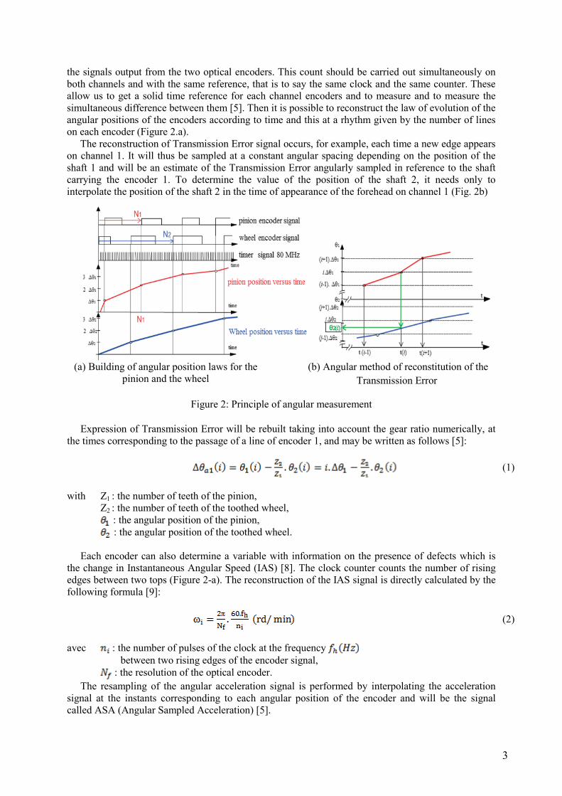
A zoom of spectrum of TSAv signal with generalized wear defect (FIG. 8), allows observing the meshing frequency and sidebands spaced at a pitch of 38.36 Hz corresponding to the average rotational speed of the primary shaft supporting the tested gears. Naturally there is a significant increase in the peak amplitude that characterizes the meshing frequency and the level of sidebands representative of modulation phenomena encountered in the power transmission gear unit [14]. It is therefore justified to take as indicators:
- The peak amplitudes of the harmonics of the meshing frequency, - And the energy of the sidebands around the harmonics of the meshing frequency. These
indicators are called harmonic modulations [15].
500 1000 15000
1000
2000
3000
4000
5000
6000
7000
8000
Frequency (Hz)
Powe
r/Fre
quen
cy
Carrier Freq = 9.6e+002 Hzsidebands Spacing = 38 Hz
Figure 8: Zoom spectra presentation of TSAv around the first harmonic of the gear mesh for General
Surface Wear pinion (GSW), (Speed: 2400 rpm, Load 11 N.m) 4. 1. 2. Analysis of Angle Sampled Acceleration ASA
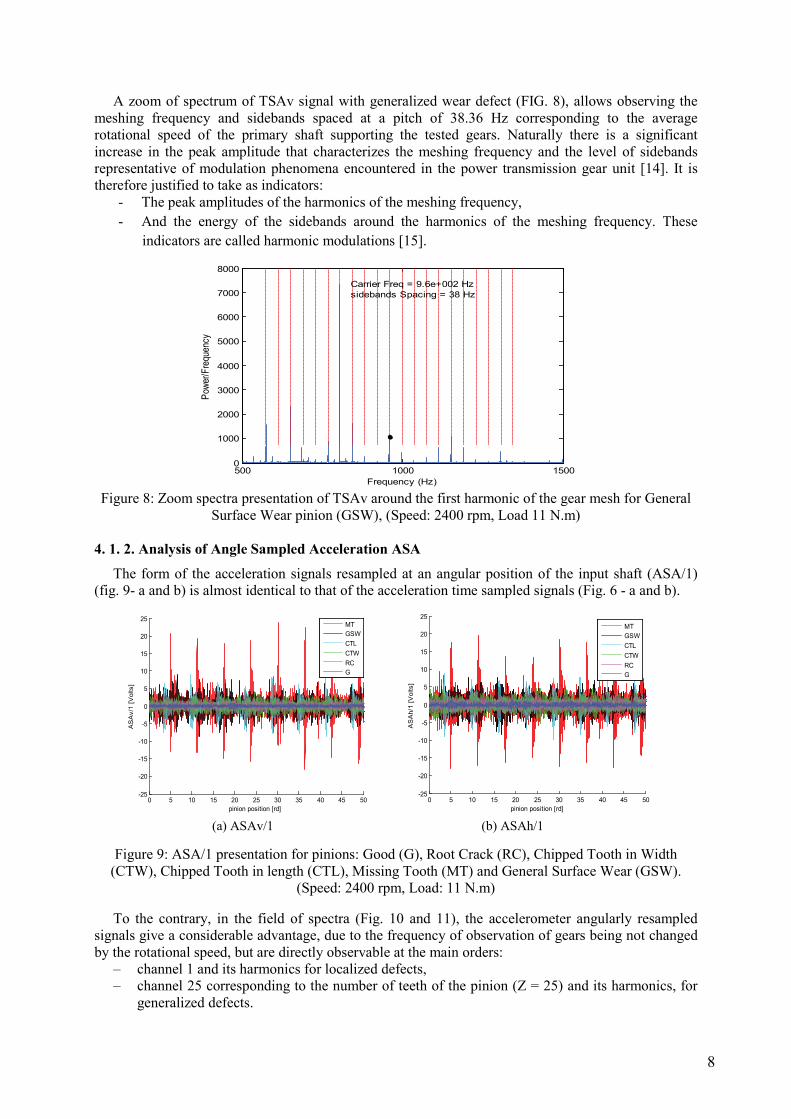
The form of the acceleration signals resampled at an angular position of the input shaft (ASA/1) (fig. 9- a and b) is almost identical to that of the acceleration time sampled signals (Fig. 6 - a and b).
0 5 10 15 20 25 30 35 40 45 50-25
-20
-15
-10
-5
0
5
10
15
20
25
pinion position [rd]
AS
Av/
1 [V
olts
]
MTGSWCTLCTWRCG
0 5 10 15 20 25 30 35 40 45 50
-25
-20
-15
-10
-5
0
5
10
15
20
25
pinion position [rd]
AS
Ah/
1 [V
olts
]
MTGSWCTLCTWRCG
(a) ASAv/1 (b) ASAh/1
Figure 9: ASA/1 presentation for pinions: Good (G), Root Crack (RC), Chipped Tooth in Width
(CTW), Chipped Tooth in length (CTL), Missing Tooth (MT) and General Surface Wear (GSW). (Speed: 2400 rpm, Load: 11 N.m)
To the contrary, in the field of spectra (Fig. 10 and 11), the accelerometer angularly resampled
signals give a considerable advantage, due to the frequency of observation of gears being not changed by the rotational speed, but are directly observable at the main orders:
– channel 1 and its harmonics for localized defects, – channel 25 corresponding to the number of teeth of the pinion (Z = 25) and its harmonics, for
generalized defects.

9
So, the presence of the fault on the pinion causes a number of events per revolution, the significant increase in the peak amplitude of the frequency channel corresponding either to the number of teeth of the pinion (Z = 25) for generalized defects, or on the frequency channel 1 for localized defects. Figures 10 and 11 show respectively the event spectra of ASA and event spectra of ASAv zoomed around principal orders: order 1 and order 25 and its harmonics (50 and 75) for the different pinions used as well as an increase in energy of the intermediate levels. It is found that the positions of these peaks will remain fixed despite variations in speed from one test to another, whereas the amplitudes vary in a different way from one frequency channel to another and depending on the type of fault. These amplitudes are subsequently used as indicators of the PV.
0 20 40 60 80 100 120
2
4
6
8
10
12
14
16
18x 10
4
X: 25Y: 1.058e+05
AS
Av/
1 [V
olts
]
X: 50Y: 3.888e+04
X: 75Y: 1.464e+05
X: 100Y: 6.919e+04
event frequency (event per revolution)
MTGSWCTLCTWRCG
0 20 40 60 80 100 120
0
0.5
1
1.5
2
2.5
3
3.5x 10
5
X: 25Y: 1.813e+05
AS
Ah/
1 [V
olts
]
event frequency (event per revolution)
X: 50Y: 1.185e+05
X: 75Y: 1.65e+05 X: 100
Y: 1.55e+05
MTGSWCTLCTWRCG
(a) Event spectra of ASAv1 (b) Event spectra of ASAh1
Figure 10: Event spectra of ASA using pinions: Good (G), Root Crack (RC), Chipped Tooth in Width
(CTW), Chipped Tooth in length (CTL), Missing Tooth (MT) and General Surface Wear (GSW). (speed: 2400 rpm, load 11 N.m)
0.97 0.98 0.99 1 1.01 1.02 1.030
2
4
6
8
10
12x 10
4
AS
Av/
1 [V
olts
]
event frequency (event per revolution)
MTGSWCTLCTWRCG
24.97 24.98 24.99 25 25.01 25.02 25.030
2
4
6
8
10
12x 10
4
AS
Av/
1 [V
olts
]
event frequency (event per revolution)
MTGSWCTLCTWRCG
49.97 49.98 49.99 50 50.01 50.02 50.030
2
4
6
8
10
12x 10
4
AS
Av/
1 [V
olts
]
event frequency (event per revolution)
MTGSWCTLCTWRCG
74.97 74.98 74.99 75 75.01 75.02 75.030
5
10
15x 10
4
AS
Av/
1 [V
olts
]
event frequency (event per revolution)
MTGSWCTLCTWRCG
Figure 11: Event spectra of ASA zoomed around principal orders (1, 25, 50 and 75) using pinions: Good (G), Root Crack (RC), Chipped Tooth in Width (CTW), Chipped Tooth in length (CTL), Missing Tooth (MT) and General Surface Wear (GSW). (Speed: 2400 rpm, load 11 N.m)

10
4. 1. 3. Transmission Error signal analysis TE
The angular sampling method in reference to the encoder 1 was used because it is the element affected by the defect, and we reconstructed the Transmission Error of the pinion from Eq. (1). The transmission Errors signals shown in Figure (12) clearly show low frequency components corresponding to the rotation speed of the shaft, and the passage of the teeth at higher frequencies. We also note that the energy depends on the type of fault.
0 5 10 15 20 25 30
-5
0
5
10
15x 10
-3
pinion position [rd]
ET(/p
ignon
) [rd]
MTGSWCTLCTWRCG
Figure 12: TE presentation for pinions: Good (G), Root Crack (RC), Chipped Tooth in Width (CTW),
Chipped Tooth in length (CTL), Missing Tooth (MT) and General Surface Wear (GSW). (Speed: 2400 rpm, Load: 11 N.m)
The orders spectra of Transmission Errors signals and their zooms shown in Figures (13 and 14) demonstrate the main orders of interest mentioned in the previous paragraph. We can say that the Transmission Error signal is a good indicator of the excitation linked to the meshing. Consequently, it is a source of building highly relevant indicators.
0 20 40 60 80 100 1200
2
4
6
8
10
12
14
X: 75Y: 0.921
X: 100Y: 1.541
X: 50Y: 1.738
X: 25Y: 13.39
Mag
nitud
e
event frequency (event per revolution)
MTGSWCTLCTWRCG
Figure 13: Event spectra of TE using pinions: Good (G), Root Crack (RC), Chipped Tooth in Width (CTW), Chipped Tooth in length (CTL), Missing Tooth (MT) and General Surface Wear (GSW).
(speed: 2400 rpm, load 11 N.m)

11
0.5 0.6 0.7 0.8 0.9 1 1.1 1.2 1.3 1.4 1.50
10
20
30
40
50
60
70
Mag
nitu
de
event frequency (event per revolution)
MTGSWCTLCTWRCG
24.5 24.6 24.7 24.8 24.9 25 25.1 25.2 25.3 25.4 25.50
5
10
15
20
25
Mag
nitu
de
event frequency (event per revolution)
MTGSWCTLCTWRCG
49.5 49.6 49.7 49.8 49.9 50 50.1 50.2 50.3 50.4 50.50
0.5
1
1.5
2
2.5
3
3.5
4
Mag
nitu
de
event frequency (event per revolution)
MTGSWCTLCTWRCG
74.5 74.6 74.7 74.8 74.9 75 75.1 75.2 75.3 75.4 75.50
0.5
1
1.5
2
2.5
3
Mag
nitu
de
event frequency (event per revolution)
MTGSWCTLCTWRCG
Figure 14: Event spectra of TE zoomed around principal orders (1, 25, 50 and 75) using pinions: Good (G), Root Crack (RC), Chipped Tooth in Width (CTW), Chipped Tooth in length (CTL), Missing
Tooth (MT) and General Surface Wear (GSW). (speed: 2400 rpm, load 11 N.m)
4. 1. 4. Instantaneous Angular Speed signals analysis IAS
The IAS signals are calculated from Eq. (2), using the encoder signal mounted on the input shaft of the gearbox where pinions with defects are mounted on. Figure 15 clearly shows the presence of a defect that is manifested by an increase in IAS.
0 5 10 15 20 25 3032
34
36
38
40
42
44
pinion position [rd]
IAS1
[Hz]
MTGSWCTLCTWRCG
Figure 15: IAS presentation for pinions: Good (G), Root Crack (RC), Chipped Tooth in Width (CTW), Chipped Tooth in length (CTL), Missing Tooth (MT) and General Surface Wear (GSW).
(Speed: 2400 rpm, Load: 11 N.m)
The event spectra corresponding to each measurement and their zooms are shown respectively on figures (16 and 17). These figures are used to track with precision the frequency components associated to the different types of defects and to the supervised geometrics (number of teeth of the pinion), whether they are localized or generalized.
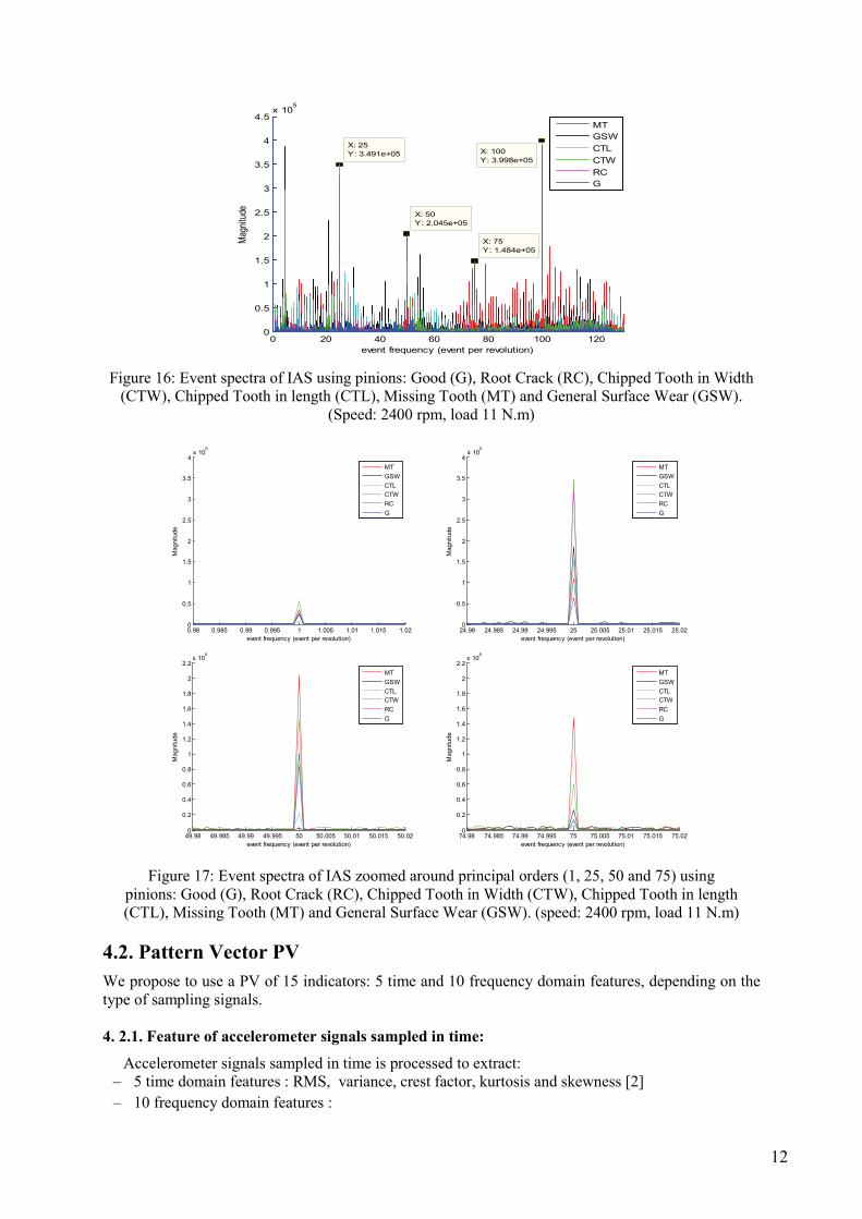
12
0 20 40 60 80 100 1200
0.5
1
1.5
2
2.5
3
3.5
4
4.5x 10
5
X: 25Y: 3.491e+05
event frequency (event per revolution)
X: 50Y: 2.045e+05
X: 75Y: 1.484e+05
X: 100Y: 3.998e+05
Magn
itude
MTGSWCTLCTWRCG
Figure 16: Event spectra of IAS using pinions: Good (G), Root Crack (RC), Chipped Tooth in Width (CTW), Chipped Tooth in length (CTL), Missing Tooth (MT) and General Surface Wear (GSW).
(Speed: 2400 rpm, load 11 N.m)
0.98 0.985 0.99 0.995 1 1.005 1.01 1.015 1.020
0.5
1
1.5
2
2.5
3
3.5
4x 10
5
Mag
nitu
de
event frequency (event per revolution)
MTGSWCTLCTWRCG
24.98 24.985 24.99 24.995 25 25.005 25.01 25.015 25.020
0.5
1
1.5
2
2.5
3
3.5
4x 10
5M
agni
tude
event frequency (event per revolution)
MTGSWCTLCTWRCG
49.98 49.985 49.99 49.995 50 50.005 50.01 50.015 50.020
0.2
0.4
0.6
0.8
1
1.2
1.4
1.6
1.8
2
2.2x 10
5
Mag
nitu
de
event frequency (event per revolution)
MTGSWCTLCTWRCG
74.98 74.985 74.99 74.995 75 75.005 75.01 75.015 75.020
0.2
0.4
0.6
0.8
1
1.2
1.4
1.6
1.8
2
2.2x 10
5
Mag
nitu
de
event frequency (event per revolution)
MTGSWCTLCTWRCG
Figure 17: Event spectra of IAS zoomed around principal orders (1, 25, 50 and 75) using pinions: Good (G), Root Crack (RC), Chipped Tooth in Width (CTW), Chipped Tooth in length (CTL), Missing Tooth (MT) and General Surface Wear (GSW). (speed: 2400 rpm, load 11 N.m)
4.2. Pattern Vector PV We propose to use a PV of 15 indicators: 5 time and 10 frequency domain features, depending on the type of sampling signals. 4. 2.1. Feature of accelerometer signals sampled in time:
Accelerometer signals sampled in time is processed to extract: – 5 time domain features : RMS, variance, crest factor, kurtosis and skewness [2] – 10 frequency domain features :
13
o the level of meshing frequency, o the level of second harmonic of meshing frequency, o the level of third harmonic of meshing frequency, o the level of meshing frequency added to the sum of the levels of twenty sidebands (10 left and
10 right of the meshing frequency), o the sum of the levels of twenty sidebands (10 left and 10 right of the meshing frequency), o the level of second harmonic of meshing frequency added to the sum of the levels of twenty
sidebands (10 left and 10 right of second harmonic of the meshing frequency), o the sum of the levels of twenty sidebands (10 left and 10 right of second harmonic of the
meshing frequency), o the level of third harmonic of meshing frequency added to the sum of the levels of twenty
sidebands (10 left and 10 right of third harmonic of the meshing frequency), o the sum of the levels of twenty sidebands (10 left and 10 right of third harmonic of the meshing
frequency), o the sum of the three first harmonic levels of meshing frequency.
4. 2.2. Feature of signals sampled in angle:
Accelerometer signals sampled in angle, Transmission Error and Instantaneous angular speed are processed to extract:
– 5 angle domain features : RMS, variance, crest factor, kurtosis and skewness – 10 ordres frequency domain features : o the level of order 1, o the level of order 25, o the level of order 50, o the level of order 75, o the level of order 100, o the sum of the levels of the 2nd to 24th order, o the sum of the levels of the 26th to 49th order, o the sum of the levels of the 51th to 74th order, o the sum of the levels of the 76th to 99th order, o the sum of the levels of the 101th to 124th order.
4.3. Designing MLP neural network for fault classification
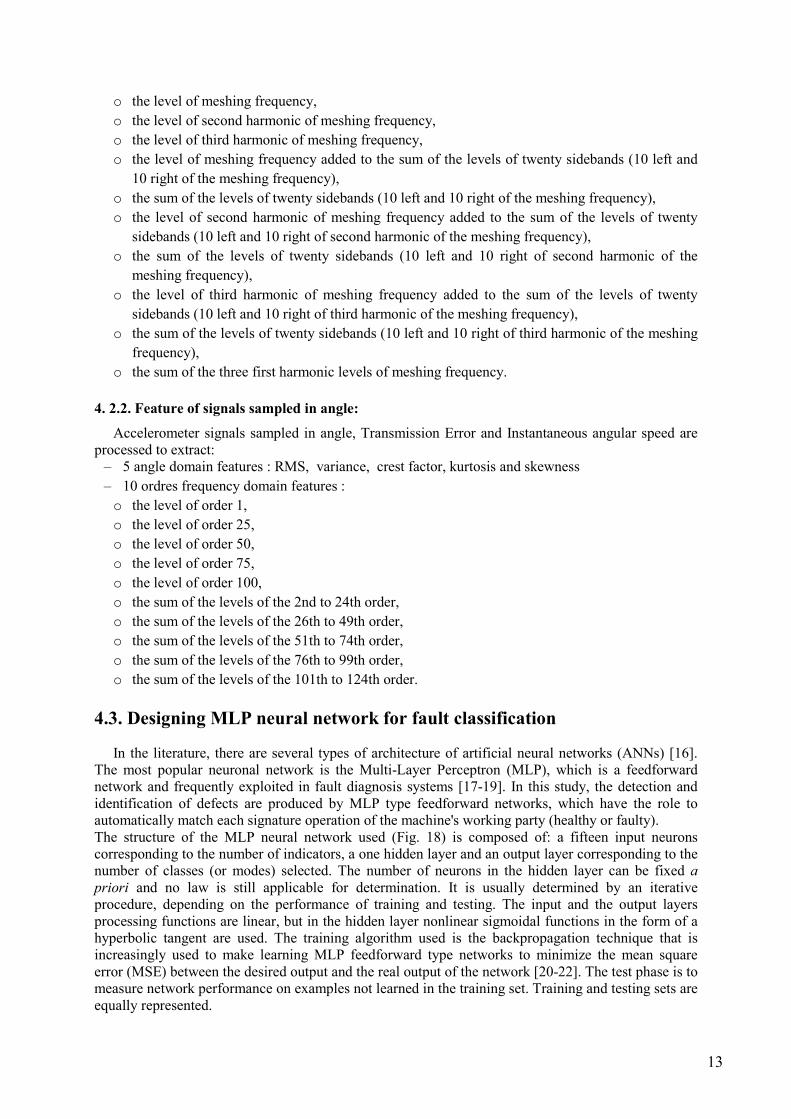
In the literature, there are several types of architecture of artificial neural networks (ANNs) [16]. The most popular neuronal network is the Multi-Layer Perceptron (MLP), which is a feedforward network and frequently exploited in fault diagnosis systems [17-19]. In this study, the detection and identification of defects are produced by MLP type feedforward networks, which have the role to automatically match each signature operation of the machine's working party (healthy or faulty). The structure of the MLP neural network used (Fig. 18) is composed of: a fifteen input neurons corresponding to the number of indicators, a one hidden layer and an output layer corresponding to the number of classes (or modes) selected. The number of neurons in the hidden layer can be fixed a priori and no law is still applicable for determination. It is usually determined by an iterative procedure, depending on the performance of training and testing. The input and the output layers processing functions are linear, but in the hidden layer nonlinear sigmoidal functions in the form of a hyperbolic tangent are used. The training algorithm used is the backpropagation technique that is increasingly used to make learning MLP feedforward type networks to minimize the mean square error (MSE) between the desired output and the real output of the network [20-22]. The test phase is to measure network performance on examples not learned in the training set. Training and testing sets are equally represented.
14
Figure 18: Schematic diagram of the MLP network
We have several types of defects, so it is important to not only detect these defects (detection phase) but also to classify them (identification phase). For this, a MLP network is specifically used at each stage of diagnosis: the detection phase, where the training set consists of examples in normal and fault conditions, so a number of neurons in the output layer equal to 2. The identification phase, where the training set consists only of examples in fault conditions, so a number of neurons in the output layer equals to 5 (5 damaged pinions). To improve the performance of MLP network, the input and output data are normalized so that they lie in the interval [-1 1]. The performance of these methods depends mainly on the relevance of the parameters of the PV selected. It is preferable to have discriminant parameters for different classes. 4.4. Classification performance
4.4. 1. Detection Phase
The network parameters are adjusted using a training set consisting of 100 vectors forms in normal condition and 500 defective conditions. Network performance is evaluated using a second base called of test (or of evaluation) like the previous. The hidden layer contains 1 to 15 neurons. Figures (19 - a and b) show the evolution of the classification rate depending on the number of neurons in the hidden layer for the different signals used. The performance of the classification using the PVs computed from the angle sampled signals is greater than those using time sampled signals. The best performances are obtained using the PVs of: TE, IAS, ASA and TSA respectively, regardless of the number of neurons in the hidden layer. For the PV of the TE we note that the classification performance is maximized when the number of neurons in the hidden layer is greater than or equal to 2. The classification rate is then higher than 99%. While for other PV performances are maximum from a number of hidden neurons greater than or equal to 11 neurons. The removal of the PVs extracted from the unload condition of training and test databases improves the performance of the classification for all types of signals used (Figure 19 - b), due to the unload operation in certain cases of gear default does not allow to discriminate them. For example, the performance of the classification with the PV of TE reaches 100% instead of 99%, when we remove the feature vectors calculated on the unload conditions from training and testing bases
.
.
.
.
.
.
Input Hidden Output
E1
E2
E3
En
S1
S2
Sn

15
(a) With the consideration of all load conditions
(b) Without consideration of the unload condition
Figure 19: MLP success rates for different number of neurons in the hidden layer
4.4. 2. Identification phase
The parameters of the network are adjusted using a base of training consisting of 75 PVs for each of the five defective operating conditions.
The results of classification by MLP represented on the figures (20- a and b) show clearly that: – the better performances are obtained when the PV is calculated starting from the angularly
sampled signals, – the best performances are obtained by using the PVs respectively of: the IAS, TE, ASA and
TSA, – the suppression of the unload mode from training and test databases makes it possible to
significantly improve the performance of classification (Figure 20-b). On the other hand, the optimum number of neurons in hidden layer was reduced at only 6 neurons.

16
(a) With the consideration of all load
conditions (b) Without consideration of the unload condition
Figure 20: MLP success rates for different number of neurons in the hidden layer
5. Conclusion In this article, we showed that starting from two accelerometers and two optical encoders, it is possible to obtain several new signals representative of the behavior of the transmission, like the Transmission Error (TE) and the Instantaneous Angular Speed (IAS) of the two shafts. The techniques of angular sampling and resampling associated to the knowledge of the laws of evolution of the angular positions of the shafts also make it possible to diversify the exploitation and the analysis carried out on the signals recorded in direct relationship with the discrete geometry in rotation (gears or bearings). Contrary to time sampling, the angular techniques are more robust to changes of operating conditions of speed or to non stationary conditions. They indeed make it possible to locate precisely and in relation to the geometrical data of the mechanical components, the frequential channels carrying information. In a general way, the results obtained in operational phases of the diagnosis by MLP neural networks, show that the best performances are obtained with the pattern vectors (PVs) built starting from the angularly sampled signals. More especially, the IAS in the identification phase and the TE in the detection phase. The angular resampling of the accelerometer signals also makes it possible to improve the performances of classification compared to time sampling. In the consequence, using angular domain features extracted from TE and IAS is recommended to diagnosis the gear faults. The removal of the PVs extracted from the signals recorded without load of the bases of training and test, makes it possible to improve the performances of classification for all the types of signals used.
17
References [1] B. Randall, Vibration-based Condition Monitoring; industrial, aerospace and automotive
applications. Editions John Wiley & Sons 2011.
[2] G. Zwingelstein, Diagnostic des défaillances. Théorie et pratique pour les systèmes industriels, Série Diagnostic et Maintenance. Editions Hermès 1995.
[3] B. Dubuisson, Diagnostic et reconnaissance des formes. Traité des nouvelles technologies. Série: Diagnostic et Maintenance. Editions Hermès, Paris 1990.
[4] G. Vachtsevanos, F.L. Lewis, M. Roemer, A.Hess, B. Wu, Intelligent Fault Diagnosis and Prognosis for Engineering Systems, John Wiley & Sons, New Jersey 2006.
[5] D. Rémond, Practical performances of high-speed measurement of gear transmission error or torsional vibrations with optical encoders. Measurement Science & Technology, Vol. 9, No. 3, (1998), pp. 347-353.
[6] F. Bonnardot, M. El Badaoui, R.B. Randall, J. Danière, F. Guillet, Use of the acceleration of a gearbox in order to perform angular resampling with limited speed fluctuation, Mechanical Systems and Signal Processing, Vol. 19, (2005), pp. 766-785.
[7] H. André, J. Antoni, Z. Daher , D. Rémond, Comparison between angular sampling and angular resampling methods applied on the vibration monitoring of a gear meshing in non stationary conditions, In Proceedings of the International Conference on Noise and Vibration Engineering, Leuven, Belgium, 2010 20-22 September.
[8] L. Renaudin, F. Bonnardot, O. Musy, J.B. Doray, D. Rémond, Natural roller bearing fault detection by angular measurement of true instantaneous angular speed, Mechanical Systems and Signal Processing, Vol. 24 (2010), pp. 998-2011.
[9] H. André, A. Bourdon, D. Rémond, Instantaneous Angular Speed monitoring of a 2MW wind turbine using a parametrization process, In Proceedings of the International Conference on Condition Monitoring of Machinery in Non-Stationary Operations, Hammamet, Tunisia, 2011 March 26-28, pp. 415-423.
[10] Y. Li, F. Gu, G. Harris, A. Ball, N. Bennett, K. Travis, The measurement of instantaneous angular speed, Mechanical Systems and Signal Processing, Vol. 19, Issue 1, (2005), pp. 786-805.
[11] S. Fedala, D. Rémond, R. Zegadi, A. Felkaoui, Utilisation de l'Erreur de Transmission et de la Variation de la Vitesse Instantanée pour le diagnostic vibratoire des défauts des engrenages, 3ième Colloque: Analyse vibratoire Expérimentale, Blois, France (2012), November 20 – 21.
[12] S. Fedala, A. Felkaoui, R. Zegadi, R. Ziani, Optimisation des paramètres du vecteur forme : application au diagnostic vibratoire automatisé des défauts d’une boite de vitesse d’un hélicoptère, J. Matériaux & Techniques, Vol. 97, No. 2, (2009)., pp. 149-155.
[13] A. Hajnayeb, A. Ghasemloonia, S. E. Khadem, M. H. Moradi, Application and comparison of an ANN-based feature selection method and the genetic algorithm in gearbox fault diagnosis, Expert Systems with Applications, Vol. 38, Issue 8, (2011), pp. 10205–10209.
[14] A. Boulenger, C. Pachaud, Analyse vibratoire en maintenance: Surveillance et diagnostic vibratoire, Technique et Ingénierie, Dunod /L'Usine Nouvelle, 2007.
18
[15] C. Fontanive, P. Prieur, Surveillance et diagnostic des engrenages, EDF, Collection de notes internes de la DER, 93NB00094.
[16] G. Drefus, J. M. Martinez, M. Samuelides, M. B. Gordon, F. Badran, S. Thiria, L. Herault, Réseaux de neurons: Méthodologie et applications. Editions Eyrolles, Paris 2002.
[17] S. Haykin, Neural networks A comprehensive foundation. 2nd ed.: Prentice Hall 1999.
[18] S. Rajakarunakaran, P. Venkumar, D. Devaraj, K. S. P. Rao, Artificial neural network approach for fault detection in rotary system, Applied Soft Computing, Vol. 8 (1), ( 2008), pp 740–748.
[19] W. Bartelmus, R. Zimroz, H. Batra, Gearbox vibration signal pre-processing and input values choice for neural network training, Artificial Intelligence Methods, Gliwice, Poland (2003) November 5–7.
[20] J. Zarei, Induction motors bearing fault detection using pattern recognition techniques, Expert Systems with Applications, Vol. 39, (2012), pp. 68–73.
[21] J. Rafiee, F. Arvani, A. Harifi, M.H. Sadeghi, Intelligent condition monitoring of a gearbox using artificial neural network, Mechanical Systems and Signal Processing, Vol. 21, (2007), pp. 1746-1754.
[22] J. C. Trigeassou, Diagnostic des machines électriques, Edition Lavoisier, Paris 2011.