Contract contingency in vertically related markets∗

Emanuele BACCHIEGA†1, Olivier BONROY‡2, and Emmanuel PETRAKIS§3

1Dipartimento di Scienze Economiche, Alma Mater Studiorum - Universita di Bologna, Italy.2INRA, Universite Grenoble Alpes, UMR GAEL, 38000 Grenoble, France.3Department of Economics, University of Crete, Rethymnon 74100, Greece.

March 8, 2017

Abstract

We study the optimal contract choice of an upstream monopolist producing an essential

input that may sell to two vertically differentiated downstream firms. The upstream

supplier can offer an exclusive contract to one of the firms or non-exclusive contracts

to both firms. Each of the latter can be made contingent or not on the breakdown

of the negotiations between the upstream supplier and the rival downstream firm. The

distribution of bargaining power during the contract terms negotiations is the main driving

force of the monopolist’s choices. A powerful supplier always opts for an exclusive contract.

By contrast, a weaker supplier offers non-exclusive contracts and makes each of them

contingent or non-contingent such as to guarantee the most favorable outside option in

its negotiations. Our main results hold under an horizontally differentiated downstream

market too.

Keywords: Vertical relationships, exclusive vs. non-exclusive relationships, contract

contingency, two-part tariff, product differentiation.

JEL classification: D43, L13, L14.

∗We wish to thank Tommaso Valletti and Christian Wey for very useful comments and discussion andthe audiences at 2016 Annual Meeting of ASSET, XXXV Jornadas de Economıa Industrial, Alicante 2015,5th EIEF-Unibo-Bocconi IGIER Workshop on Industrial Organization, Rome 2015 and CORE@50 conference,Louvain-la-Neuve, 2016. The usual disclaimer applies.†Bemanuele.bacchiega@unibo.it‡Bolivier.bonroy@inra.fr§Bpetrakis@uoc.gr

1

1 Introduction

The bulk of final products in the market has passed through various production stages. Verti-

cal relations, and in particular vertical contracting, is thus of crucial importance for the final

good prices, the profitability of firms along the vertical supply chain, the consumer surplus

and the social welfare. Vertical contracting refers not only to the type of contracts used in

the trading between upstream and downstream firms, but also to the process via which the

specific contractual terms are determined. There is a variety of contract types used in the real

world. In some industries firms use simple linear wholesale price contracts in their trading, yet

in others the contract types are more complicated.1 In addition, there is strong evidence that

the trading terms of these contracts are negotiated among upstream and downstream firms.2

This is mainly due to the recently observed increased concentration in many downstream

sectors that has transformed downstream firms to powerful actors.3

In this paper we investigate the optimal contact choices of an upstream monopolist that

may sell an essential input to downstream firms that produce vertically differentiated prod-

ucts. Once the contracts have been selected, their terms are negotiated between the upstream

supplier and the downstream firm(s). Assuming that contracts take the form of two-part

tariffs, we inquire into the following issues. Does the upstream supplier have incentives to

foreclose one of the downstream firms by offering an exclusive contract to the other firm?

And if so, the foreclosed firm will be the high- or the low-quality one? When the upstream

firm offers non-exclusive contracts to both downstream firms, what will be the specific type of

these contracts? Under what conditions, will it offer a contingent contract that allows renego-

tiation of contract terms with one downstream firm in case of breakdown in the negotiations

with the other one?4 Or when will it offer a non-contingent contract not allowing for such

renegotiations? What are the market and societal implications of the upstream monopolist

contract configuration selection?

We consider a vertically related industry with an upstream monopolist and (potentially)

two downstream firms. The upstream supplier produces an essential input that sells to one

or both downstream firms, depending on its decision at the outset of the game to offer an

exclusive or two non-exclusive contracts, respectively. The downstream firms are endowed

1For empirical studies regarding the contract types used see e.g., Villas-Boas (2007), Thanassoulis andSmith (2009) and Bonnet and Dubois (2010). In addition, in the case of grocery retailing anecdotal evidenceindicates the use of very complex contracts that avoid double marginalization (see Inderst and Mazzarotto,2008).

2For evidence of bargaining among milk suppliers and supermarkets see Thanassoulis and Smith (2009). Inaddition, there is evidence that large retailers, such as Wal-Mart bargain with product suppliers, large bookretailers, such as Barnes & Noble, bargain with publishers, large tour operators bargain with hotels.

3The increase in downstream concentration has been noted in a number of policy reports (see e.g. EuropeanCommission, 1999, OECD, 1999, and FTC, 2001).

4According to (Bazerman and Gillespie, 1998, p. 155), “the terms of a contingent contract are not finalizeduntil the uncertain event in question–the contingency–takes place.”

2

with different technologies that allow the production of different output qualities using the

same input (see Gabszewicz and Thisse, 1979; Shaked and Sutton, 1983).5 If the upstream

supplier chooses to offer contracts to both downstream firms, it must also decide whether

each of them is contingent or non-contingent. A contingent contract is more flexible and

allows negotiating parties to set different contractual terms in case of agreement and in case

of disagreement in the rival bargaining pair. This flexibility is absent under a non-contingent

contract.

We study a three-stage game with observable actions. In the first stage, the upstream

monopolist decides to offer an exclusive contract or two non-exclusive ones. In the former case,

it also decides to which of the downstream firms to make the offer. In the latter case, it also

decides the configuration of contracts to be offered, i.e., two contingent, two non-contingent,

or mixed (one contingent and another non-contingent) contracts. In legal terms, this can be

materialized by using a letter of intent wherewith the upstream firm sets out its intentions

about the number and type of contractual relations to enter.6 In the second stage, negotiations

over contract terms take place between the upstream monopolist and the downstream firm(s).

In case of non-exclusive contracts, these negotiations take place simultaneously and separately

between the upstream supplier and each of the downstream firms. In the last stage, under

non-exclusive contracts, the downstream firms compete in the market by selecting their prices

or their quantities; under an exclusive contract, the downstream monopolist sets its price.

As the alternative types of non-exclusive contracts are central in our analysis, a discussion

in detail of their features will be of great help for the sequel. A non-exclusive contract signed

between the upstream supplier and a downstream firm can be of two types: contingent and

non-contingent. A contingent contract contains specific terms in the event of a breakdown in

the negotiations in the rival bargaining pair. An immediate consequence is that the outside

options for the negotiating firms fully internalize the implications of the negotiation failure

in the rival pair. By contrast, a non-contingent contract does not allow for renegotiation of

contract terms in case of a breakdown in the negotiations in the rival bargaining pair. As a

consequence, the outside options for the negotiating firms are determined by their equilibrium

contractual terms.Therefore, the crucial difference between the two types of non-exclusive

contracts lies on the outside options that are attributed to negotiating parties under each of

them (see e.g., Milliou and Petrakis (2007)).

5For instance, one of the downstream firms has a proprietary technology that allows it to increase at nocost the quality of its good.

6With a letter of intent, a party sets forth its intention to sign a contract in the circumstances reported inthe letter. It is worth noticing that “A letter of intent is not itself a formal contract but certain of its provisions(e.g. concerning payment for any work completed) may nevertheless be enforceable. Letters of intent are widelyused in the UK construction industry, where their usual purpose is to encourage a contractor to begin workon a time-sensitive project before legal formalities have been completed. Recent case law suggests that thecourts are increasingly willing to find that a letter of intent constitutes a binding contract, provided that allnecessary elements of a contract are present [. . . ]” Law (2016).

3

Our analysis highlights the role of the bargaining power distribution between the upstream

supplier and each of the downstream firms for the optimal selection of contracts. In particu-

lar, when the upstream supplier is quite powerful, it offers an exclusive contract to the high

quality downstream firm, whereas it selects two non-exclusive contracts when its bargaining

power is not too high. The upstream supplier faces the following trade-off when selecting

between an exclusive and two non-exclusive contracts. Under an exclusive contract, competi-

tion downstream is absent altogether, therefore, under two-part tariff contracts, the vertically

integrated structure outcome is obtained. Yet, the upstream supplier’s outside option (i.e.,

its profits when the negotiations with the downstream firm break down) is nil in this case.

This entails that its share of the vertically integrated entity’s profits is proportional to the

upstream bargaining power. The lower the latter, the smaller the profit that the upstream

supplier is able to extract. By contrast, with non-exclusive contracts that are negotiated si-

multaneously and separately, competition downstream erodes part of the aggregate producer

surplus (O’Brien and Shaffer, 1992). Yet, with non-exclusive contracts, the upstream sup-

plier may have a stronger bargaining position, i.e., it may enjoy positive outside options in

its negotiations with the downstream firms, for any level of its bargaining power. A powerful

upstream firm can extract most of the vertically integrated structure’s profit and prefers, thus,

to avoid creating downstream competition that reduces the aggregate producers surplus. In

addition, as the production of the high-quality good generates a higher surplus, the upstream

opts to offer the contract to the high quality downstream firm. In this way, the upstream

supplier forecloses the low-quality firm.

As the upstream supplier becomes less powerful, it can extract a lower share of the verti-

cally integrated structure. Nonetheless, by offering two non-exclusive contracts, the upstream

supplier can enjoy a stronger bargaining position through the creation of outside options in its

negotiations with the downstream firms (of course, this comes at the cost of reducing the ag-

gregate producer surplus due to downstream competition). In particular, for “intermediate”

levels of bargaining power, the upstream firm opts for two non-exclusive, contingent contracts,

whereas for even lower values of it, it offers a non-contingent contract to the high-quality down-

stream firm and a contingent contract to the low-quality one. Finally, an upstream supplier

with quite low bargaining power opts for two non-exclusive, non-contingent contracts. As dis-

cussed above, a contingent contract is more flexible in the sense that it allows a negotiating

pair to specify different contract terms in case of agreement and in case of disagreement in the

rival bargaining pair. This translates into higher outside options for the upstream supplier

under contingent than under non-contingent contracts, but only if its bargaining power is not

too low. The opposite holds for lower values of the upstream bargaining power, in which case

the upstream supplier opts for one or two non-contingent contracts. In the mixed contract

configuration, the non-contingent contract is always offered to the high-quality firm. In this

4

way, the upstream supplier enjoys the largest outside options once again. Finally, our analy-

sis reveals that the degree of vertical product differentiation affects the upstream supplier’s

choice of the configuration of non-exclusive contracts. In particular, as the goods become less

differentiated, the range of parameters for which the upstream supplier offers mixed contracts

shrinks; moreover, that non-contingent contracts are more often selected when the product

differentiation takes intermediate values.

Interestingly, the fixed fees of the equilibrium non-exclusive contracts are sometimes neg-

ative, i.e., the upstream supplier pays “slotting allowances” (Shaffer, 1991; Marx and Shaffer,

2010) to one or both downstream firms. This is always true when the upstream supplier offers

two non-contingent contracts. It is also true under contingent and mixed contracts as long as

the upstream bargaining power is low enough. Surprisingly, under some circumstances, the

contract offered to the low-quality firm generates an overall loss for the upstream supplier.

This loss is however covered by a substantial gain for the upstream supplier that so enjoys a

stronger bargaining position vis-a-vis the high-quality downstream firm.

Our main findings carry on, to a major extent, when downstream firms compete in quanti-

ties, instead of prices. There are, however, two points of departure. First, two non-exclusive,

non-contingent contracts are never observed in equilibrium. This is because the outside op-

tions they imply for the upstream supplier are lower than under contingent contracts, con-

firming thus the intuition of the price setting market. And second, the degree of vertical

product differentiation now plays a crucial role. Mixed contracts are never observed in equi-

librium when the goods are not differentiated enough . Moreover, an exclusive contract to

the high-quality firm is selected by the upstream supplier even if its bargaining power is low,

provided that the goods are not too differentiated.

Finally, we show that our main findings are not specific to the vertical product differen-

tiation setup, but hold also in an horizontally differentiated model in which a representative

consumer has a Bowley (1924), Spence (1976), Dixit (1979) utility function. The main depart-

ing point in this case is that exclusive contracts are observed in equilibrium only if the goods

are close substitutes. When the goods are poor substitutes, the upstream supplier prefers

to strengthen its bargaining position by offering non-exclusive, contingent contracts to both

downstream firms.

Our paper connects to several strands of the literature. First, it contributes to the litera-

ture on vertical contracting. A main theme within this literature is the commitment problem

that arises for an upstream monopolist when it trades with multiple competing downstream

firms (see, e.g. Horn and Wolinsky, 1988; O’Brien and Shaffer, 1992; McAfee and Schwartz,

1994, 1995; Rey and Verge, 2004). These papers, however, do not consider the optimal choice

of contracts offered by the upstream supplier to the downstream firms. Our paper undertakes

this task and highlights the differential impact of contingent and non-contingent, non-exclusive

5

contracts on the severity of the upstream monopolist’s commitment problem. Based on that,

we are able to identify conditions under which an upstream monopolist offers an exclusive or

two non-exclusive contracts, and within the non-exclusive contracts when it offers contingent,

non-contingent and mixed contracts to the downstream firms.

It also contributes to the literature on the effects of countervailing buyer power (see, e.g.

Inderst and Wey, 2003, 2007). More closely related to our analysis is the paper by Milliou

and Petrakis (2007). Their focus is on merger incentives when upstream supplier(s) choose(s)

optimally the contracts to be offered to the downstream firms. They consider the choice

between wholesale price and two-part tariff contracts, assuming though that these contracts

are non-contingent. By contrast, we consider two-part tariff contracts and highlight that the

contingency or non-contingency of their terms is crucial for the selection of contracts by the

upstream monopolist. As in Milliou and Petrakis (2007), upstream and downstream firms ne-

gotiate over contract terms, with the bargaining power distribution among negotiating parties

to be exogenously given.7 Further, Miklos-Thal et al. (2011) consider powerful downstream

retailers offering take-it-or-leave-it contracts to an upstream supplier that may be contin-

gent on an exclusive relationship, and show that contingency may lead to the replication of

monopoly outcomes. From another standpoint, Iozzi and Valletti (2014) delve into the role of

the observability of negotiations breakdown in determining the outside option of an upstream

supplier facing multiple downstream retailers, when negotiations are determined through the

generalized Nash bargaining solution.

Our paper also contributes to the literature on vertical foreclosure. Hart and Tirole (1990),

O’Brien and Shaffer (1992), and McAfee and Schwartz (1994) show that under secret contract-

ing, exclusive agreements or vertical integration can help a dominant supplier to reestablish

its market power. Rey and Tirole (2007) provide an excellent overview on vertical foreclosure

and stress the anticompetitive motives for upstream firms to use exclusive agreements and

vertical mergers in order to foreclose downstream firms. The received literature, however,

does not consider vertically differentiated industries. In line with this literature, we show

that an upstream monopolist opts for an exclusive contract with the high-quality downstream

firm, thus foreclosing the low-quality one, in order to restore its market power. Nevertheless,

this is optimal for the supplier only when its bargaining power is sufficiently high. Otherwise,

the upstream supplier has incentive to keep both competing downstream firms in the market.

Finally, our paper contributes to the debate regarding the choice of a firm to offer or not

a pooling or a separating menu in markets of vertical product differentiation, see Acharyya

(1998), Bacchiega et al. (2013) and Chambolle and Villas-Boas (2015). These papers consider

either a monopolist selling to heterogeneous consumers different qualities of a good or two

7In a different vein, Alipranti et al (2014), assuming negotiations over two-part tariff non-contingent con-tracts between an upstream supplier and two downstream firms, compare Cournot and Bertrand downstreamcompetition.

6

upstream suppliers offering different qualities of products to a monopolist retailer or to two

competing retailers. In contrast, we assume that the downstream market is vertically differen-

tiated, whereas the essential input produced by the upstream supplier is homogeneous. In line

with this literature, we identify circumstances under which the upstream monopolist offers the

same or different types of non-exclusive contracts to both downstream firms. In particular,

when the upstream bargaining power is relatively low (but not too low), the supplier opts for

a contingent contract to the low-quality downstream firm and a non-contingent contract to

the high-quality one.8

The remainder of the paper is organized as follows. Section 2 presents the model, Section

3 explores the various contractual choices and Section 4 performs the contractual choice

equilibrium analysis. Section 5 discusses the equilibrium outcomes. Section 6 explores the

robustness of our results. Finally, Section 7 provides concluding remarks.

2 The model

2.1 Firms and market structure

Consider an upstream monopolist, denoted by U , producing at no cost an essential input

that may sell to two downstream firms. Downstream firms use this input to produce, on a

one-to-one basis, a final good. Besides the input costs, downstream firms incur no additional

production costs. One of these firms has a proprietary technology that allows it to increase

at no cost the quality of its good. Denote the latter “high-quality good” and the downstream

producer “high-quality firm”, Dh. The other downstream firm, the “low-quality firm”, Dl,does not dispose such a technology and thus produces the “basic” version of the good, i.e., the

“low-quality good”. The upstream monopolist decides whether to offer an exclusive supply

contract and if so, to which of the downstream firms to make the offer. Under an exclusive

contract the upstream monopolist commits to trade with one downstream firm alone, therefore

the downstream market is a monopoly.

By contrast, if the upstream supplier chooses to sign non-exclusive contracts, it trades

with both downstream firms and thus the downstream market is a vertically differentiated

duopoly. Non-exclusive contracts can be of two types: non-contingent and contingent. Con-

tingent contracts allow bargaining partners U and Di to renegotiate the contract in case of

disagreement between U and Dj . Under non-contingent contracts, the bargaining partners

should stick to their negotiated contract terms under all contingencies. The upstream supplier

8From a broader perspective, our viewpoint of contract contingency as an instrument to affect the bargainingposition of the negotiating parties is alternative to those suggested in the economic literature, in which contractcontingency is seen as a tool to reduce the incompleteness of contracts (see, e.g. Hart and Holmstrom, 1987),and in the management literature, in which it is seen as a tool to share risks (Byialogorsky and Gerstner,2004).

7

decides which type of non-exclusive contract to offer to each downstream firm.9

Vertical contracts are non-linear and in particular, take the form of two-part tariffs, and

are bargained between the upstream monopolist and the downstream firm(s). During the

contract negotiations, the bargaining power of U and Di, i = h, l, are µ and 1−µ, 0 ≤ µ ≤ 1,

respectively.

2.2 Demand

A continuum of heterogeneous consumers of unit mass is uniformly distributed with unitary

density over the interval [0, 1]. A consumer θ, θ ∈ [0, 1], is characterized by the indirect utility

function

U(θ, ui) =

θui − pi when buying one unit of good i,

0 otherwise(1)

where ui is the (given) quality level of good i and pi is its price. Remember that ui only

depends upon the downstream firm selling the good.

Under an exclusive contract, there is only one good available in the market. Using the

standard marginal consumer approach, its demand is

Dm(pm) = 1− pmui, (2)

where the subscript m indicates “downstream monopoly” and i = h, l, depending on which

downstream firm the supply contract has been signed with. In this case, the consumer surplus

is

CSm(pm) =

∫ 1

pmui

(θui − pm)dθ. (3)

Under non-exclusive contracts, two goods are available in the market. Using again the stan-

dard marginal consumer approach,10 their demands are

Dh(ph, pl) = 1− ph − pluh − ul

, Dl(ph, pl) =ph − pluh − ul

− plul, (4)

with uh > ul > 0 being the quality levels of the two goods. The consumers surplus is

9This may be materialized by writing a letter of intent which contains the number and - in case of nonexclusivity - the type of contractual relationships which the upstream supplier is willing to enter. Contractsmay then be made contingent by including in such letters the appropriate conditions precedent.

10The consumer which is indifferent between buying the high or the low quality good is determined byθhluh − ph = θhlul − pl; and the consumer which is indifferent between buying the low quality good or notbuying at all is determined by θl0ul − pl = 0.

8

CS(ph, pl) ≡∫ ph−pl

uh−ul

plul

(θul − pl)dθ +

∫ 1

ph−pluh−ul

(θuh − ph)dθ. (5)

2.3 Timing

We consider a three-stage game with observable actions. At the first stage, the upstream

supplier decides whether to offer an exclusive contract, and if so, to which of the downstream

firms. If, instead, it decides to offer non-exclusive contracts, the upstream supplier selects

also whether to make each of these contracts contingent or non-contingent. In addition, it

decides whether or not to offer the same type of contract to both downstream firms. In

case that the two contracts differ, the upstream supplier decides whether to offer, e.g., the

contingent contract to the low or the high quality downstream firm. At the second stage,

the upstream monopolist and the downstream firm(s) bargain (simultaneously) over two-part

tariff contract(s). Finally, the downstream firm(s) set price(s) in the market.11

As is standard, we use subgame perfection to solve our three-stage game. Moreover, we

invoke the Nash equilibrium of simultaneous generalized Nash bargaining problems to solve

for the simultaneous contract terms negotiations between U and each of Di, i = h, l, under

non-exclusive contracts. Under exclusive contracts, the generalized Nash bargaining solution

is also used to solve for the contract terms negotiations between U and one of the downstream

firms.

3 Contract terms and market outcomes

In the next subsections, we analyze the subgames in which the upstream monopolist offers

respectively an exclusive contract or two non-exclusive contracts. In the latter case, we

distinguish between the symmetric cases in which both downstream firms are offered either

non-contingent or contingent contracts and the mixed cases of one downstream firm being

offered a contingent and the other a non-contingent contract.

3.1 Exclusive contract

Under an exclusive contract, the downstream firm to which the upstream supplier offers the

contract becomes a monopolist in the final good market. Let Tm ≡ (wm, tm) be the two-

part tariff contract signed by the upstream and the downstream firm, where wm is the input

price and tm is the fixed fee, with m standing for downstream monopoly. The profits of the

11Section 6 deals with the alternative case in which firms compete in quantities.

9

upstream and downstream firms are, respectively

Πm(pm, Tm) = Dm(pm)wm + tm, πm(pm, Tm) = Dm(pm)(pm − wm)− tm. (6)

In the last stage, the downstream firm maximizes its profit by setting pm(wm) = ui+wm2 .

Substituting the latter into (6), we obtain downstream and upstream equilibrium profits

Πm(Tm) = (ui−wm)wm2ui

+ tm (7)

and

πm(Tm) = (ui−wm)2

4ui− tm. (8)

Turning to the second stage, the upstream supplier and the downstream firm negotiate over

the contract terms. As the upstream supplier is committed to offer an exclusive contract, in

case of failure to reach an agreement neither the upstream nor the downstream firm operate

in the market; hence both firms’ outside options are nil. The generalized Nash product is,

therefore,

NPm(Tm) = Πm(Tm)µπm(Tm)1−µ. (9)

The maximization of (9) with respect to wm and tm yields w∗m = 0 and t∗m = ui4 µ. As standard

in this case, the two-part tariff contract is set in such a way as to maximize the joint profit of

the vertical chain. This is achieved by setting the input price equal to the upstream marginal

cost and by apportioning the maximum joint profit between the upstream and downstream

firm via the fixed fee, according to their respective bargaining powers. Therefore, the profits

accruing to the upstream firm are ui4 µ and are increasing in the quality of the good ui. As

a consequence, the upstream supplier will offer the exclusive contract to the high quality

downstream firm. The following Lemma summarizes our findings.

Lemma 1. If the upstream supplier opts for an exclusive contract, it offers it to the high

quality downstream firm. The equilibrium contract terms are w∗m = 0 and t∗m = uh4 µ. The

equilibrium price is p∗m = uh2 ,the equilibrium demand is D∗m = 1

2 , and the equilibrium profits

of the upstream and downstream firms are, respectively, Π∗m = uh4 µ and π∗m = uh

4 (1 − µ).

Moreover, the consumer surplus is CS∗m = uh8 .

3.2 Non-exclusive non-contingent contracts

We now turn to the case in which the upstream monopolist offers supply contracts to both

downstream firms. For the sake of brevity, we will often refer to the contract signed between

the upstream supplier and the high (low) quality downstream firm as “the high (low) quality

contract”.We assume that negotiations over contract terms within each (U ,Di) pair occur

10

simultaneously and separately, and that the contracts are interim observable, i.e., once the

contracts have been signed, their terms become known to all the parties (see e.g., McAfee

and Schwartz, 1995). It is well-known that in such a situation, the vertical relations between

the upstream supplier and each of the downstream firms are affected by opportunism. In

particular, within each (U ,Di) negotiating pair, an incentive exists to secretly renegotiate the

contract terms at their own advantage and at the expense of the rival downstream firm j

(i, j = h, l, i 6= j). One of the consequences is that multiple equilibria may arise in this case.

To deal with this issue and obtain a unique outcome, we invoke pairwise proofness in the

equilibrium contracts (O’Brien and Shaffer, 1992; Milliou and Petrakis, 2007; Alipranti et al.,

2014).

In this subsection, we consider that the upstream supplier offers non-contingent contracts

to both downstream firms, while the case of contingent and mixed contracts will be analyzed

in the following two subsections. A contract between U and Di is non-contingent if its terms

remain intact independently whether the (U ,Dj) negotiating pair reaches or not an agreement.

Stated differently, the (out-of-equilibrium) occurrence of breakdown in the negotiations be-

tween the upstream supplier and the downstream firm j does not initiate negotiations anew

between U and Di, instead the (U ,Di) pair abides with its agreed contract terms. By contrast,

a contract is contingent when it specifies different contract terms for the case of agreement

and for the case of disagreement in the rival bargaining pair. For a thorough discussion of

contract contingency see Milliou and Petrakis (2007).

In the last stage, given the demand system in (4) and the contracts Ti ≡ (wi, ti) signed be-

tween the upstream supplier and the downstream firm i, i = h, l, the profits of the downstream

firm i and the upstream supplier are

πi(ph, pl, Ti) = Di(ph, pl)(pi − wi)− ti, i = h, l, (10)

Π(ph, pl, Th, Tl) = Dh(ph, pl)wh +Dl(ph, pl)wl + th + tl. (11)

Solving the system of equations defined by the first-order conditions ∂πi(·)∂pi

= 0 and ob-

serving that the second-order conditions are satisfied as long as uh > ul > 0, it is easy to

obtain the equilibrium prices

ph(wh, wl) =uh[2(uh − ul + wh) + wl]

4uh − ul, pl(wh, wl) =

ul(uh − ul + wh) + 2uhwl4uh − ul

. (12)

Substituting (12) into (10) and (11), the equilibrium downstream and upstream profits

11

are

πh(Th, wl) =

[2u2h + uh(wl − 2(ul + wh)) + ulwh

]2(uh − ul)(4uh − ul)2

− th, (13)

πl(Tl, wh) =uh [uh(ul − 2wl) + ul(wh + wl − ul)]2

ul(uh − ul)(4uh − ul)2− tl, (14)

Π(Th, Tl) =ulϑ+ uhulwl(uh − ul + 2wh) + uhw

2l (ul − 2uh)

ul(uh − ul)(4uh − ul)+ th + tl, (15)

with ϑ =[w2h(ul − 2uh) + 2uhwh(uh − ul)

].

We next turn to the bargaining stage. As noted above, in the case of non-contingent

contracts, say, the (U ,Dh) pair cannot include in their bargaining agenda contract terms that

will be executed only in the (out-of-equilibrium) case of negotiations breakdown between Uand Dl.This entails that the outside option for the upstream monopolist when bargaining with

downstream firm i depends on the equilibrium contract terms signed with firm j.

Let TNi ≡ (wNi , tNi ), i = h, l, be the equilibrium non-contingent contract signed within

the (U ,Di) pair. In the bargaining with, say, firm Dh, the outside option of the upstream

monopolist is the profit it would earn in case of negotiations breakdown with firm Dh itself.

Should this occur, the upstream supplier still expects to sign the contract TNl with down-

stream firm Dl, which, however, will be a monopolist in the final good market. The outside

option for the upstream monopolist is, therefore, Πm(TNl ), whereas the outside option for the

downstream firm Dh is zero (Similarly, for the bargaining between U and Dl).12 Accordingly,

the generalized Nash products are

NPNh (Th, TNl ) =

[Π(Th, T

Nl )− Πm(TNl )

]µπh(Th, w

Nl )1−µ, (16)

NPNl (TNh , Tl) =[Π(TNh , Tl)− Πm(TNh )

]µπl(Tl, w

Nh )1−µ. (17)

12Inderst and Wey (2003); de Fontenay and Gans (2005) develop an explicit strategic bargaining game tomodel the idea that the negotiation between parties can come to a breakdown.

12

Standard maximization techniques allow us to find the equilibrium non-contingent contracts13

TNh = (wNh , tNh ) =

(ul4,8µu3h − 4(1 + µ)u2hul + 2(1− µ)uhu

2l − (1− µ)u3l

32u2h

), (18)

TNl = (wNl , tNl ) =

(u2l

4uh,ul[2µuh − (3− µ)ul]

32uh

). (19)

Substituting the above back into prices, demands and profits yields the following result.

Lemma 2. If the upstream supplier offers non-contingent contracts to both downstream firms

then the equilibrium contract terms are (18) and (19). The equilibrium prices are pNh = 2uh−ul4

and pNl = ul4 , and the equilibrium demands DN

h = 12 and DN

l = 14 . The equilibrium profit of

the upstream monopolist is ΠN =8µu3h−2µu

2hul+(1−µ)uhu2l−(1−µ)u

3l

32u2h, and those of the downstream

firms are πNh = (1−µ)(2uh−ul)2(2uh+ul)32u2h

and πNl = (1−µ)ul(2uh+ul)32uh

. Finally, the consumer surplus

is CSN = uh8 + 5

32ul.

3.3 Non-exclusive contingent contracts

Contingent contracts capture the idea that bargaining pairs can come to a permanent and

irrevocable breakdown in their negotiations (see, e.g. Inderst and Wey, 2003; de Fontenay

and Gans, 2005). Therefore, a contingent contact between the upstream monopolist and the

downstream firm i contains specific terms that will be executed in case that the negotiations

between U and Dj breakdown. In such a case, the downstream firm i becomes a monopolist

in the final good market and the upstream supplier’s profit is as under exclusive contracts,

namely, ui4 µ (see subsection 3.1). The latter is thus the outside option of the upstream supplier

in the bargaining with the downstream firm i, while the outside option of the downstream

firm is again nil.

As the last stage of the game is unaffected by the contingency or not of the contracts (see

subsection 3.2 for last stage equilibrium outcomes), the generalized Nash products are

NPCh (Th, TCl ) =

[Π(Th, T

Cl )− ul

4µ]µπh(Th, w

Cl )1−µ, (20)

NPCl (TCh , Tl) =[Π(TCh , Tl)−

uh4µ]µπl(Tl, w

Ch )1−µ. (21)

where TCi ≡ (wCi , tCi ), i = h, l, is the equilibrium contingent contract signed between U and

Di.13Maximizing first each generalized Nash product NPNi (·) w.r.t. ti, then plugging the solution back into

NPNi (·), we end up with an expression proportional to the excess joint profits of the (U ,Di) pair. Thenmaximizing these excess joint profits w.r.t. wi and solving the system of the first order conditions, we obtain theequilibrium contract terms. Second-order conditions are locally satisfied, which, together with the uniquenessof the maximizers, insures the uniqueness of the solution. The detailed (and cumbersome) calculations areavailable upon request.

13

Unlike in the case of non-contingent contracts, concavity of the functions (20) and (21)

at the critical points identified by the first order conditions (focs) is not always guaranteed.

Nevertheless, a sufficient condition that guarantees concavity at the unique solution of the

system of the focs is that µ ≤ 34 . In fact, if 3

4 < µ ≤ 1, the profit of the low quality downstream

firm at the solution of the focs turns out to be negative, thereby violating its participation

constraint. Here we will focus on the analysis of the interior solution, relegating that of the

corner solution (34 < µ ≤ 1) to the Appendix 1. As we will see, offering two contingent

contracts in this latter case turns out to be a dominated strategy for the upstream supplier.

Let µ ≤ 34 . Using standard maximization techniques,14 we obtain the equilibrium contracts

TCh = (wCh , tCh ) =

(ul4,4µ(2− µ)uh − (3 + µ)ul)

16(2− µ)

), (22)

TCl = (wCl , tCl ) =

(u2l

4uh,ul[(−1 + 6µ− 4µ2)uh − (2− µ)ul]

16(2− µ)uh

). (23)

The following Lemma summarizes our findings.

Lemma 3. If the upstream supplier offers contingent contracts to both downstream firms then:

(i) If µ ≤ 34 , the equilibrium contract terms are given by (22) and (23). The equilibrium

prices are pCh = 2uh−ul4 , pCl = ul

4 , and the equilibrium demands are DCh = 1

2 , DCl = 1

4 .

The equilibrium profits of the upstream monopolist are ΠC = µ[4uh−ul+4(1−µ)(uh+ul)]16(2−µ) and

those of the downstream firms are πCh = (1−µ)[4uh(2−µ)−5ul]16(2−µ) and πCl = ul(1−µ)(3−4µ)

16(2−µ) . The

consumer surplus is CSC = uh8 + 5

32ul.

(ii) If 34 < µ ≤ 1, the upstream supplier should adjust the fixed fee downwards in order to

incentivize the low-quality firm to sign the contract. Non exclusive contingent contracts

are, however, dominated by an exclusive contract offered to the high-quality downstream

firm.

3.4 Non-exclusive mixed contracts

In this subsection we consider the case in which the upstream supplier offers a non-contingent

contract to one downstream firm and a contingent contract to the other one. In what follows,

we focus on the analysis of the case in which the contingent contract is offered to the low-

quality downstream firm and the non-contingent contract to the high-quality one. As is shown

in the Appendix 2, the reverse case is always dominated by the upstream supplier offering

contingent contracts to both downstream firms.

14see footnote 13.

14

When Dl is offered a contingent contract, Dh knows that in case of a breakdown in its

negotiations with the upstream supplier, U and Dl will behave as a chain of monopolies.

Therefore, the outside option for the upstream supplier in the negotiations with the high

quality downstream firm is µul4 . Conversely, the outside option for U in the negotiations with

Dl stems from the fact that its contract with Dh cannot include clauses that are contingent

on the disagreement between U and Dl itself. Letting TMi ≡ (wMi , tMi ) be the equilibrium

contract signed between U and Di, i = h, l, the generalized Nash products are

NPMh (Th, TMl ) =

[Π(Th, T

Ml )− ul

4µ]µπh(Th, w

Ml )1−µ, (24)

NPMl (TMh , Tl) =[Π(TMh , Tl)− Πm(TMh )

]µπl(Tl, w

Mh )1−µ. (25)

As in the case of contingent contracts, the generalized Nash products (24) and (25) are not

always concave at the solution of the system of the first-order conditions. In particular,

the concavity of NPMh (·) is guaranteed either when uluh≤ 4

5 or when uluh

> 45 and µ ≤

8u2h−4uhul−u2l

ul(6uh−ul) < 1.15

In this parameter constellation, standard maximization techniques16 lead to the equilib-

rium contracts

TMh = (wMh , tMh ) =

(ul4,8µu2h − 2

(3µ2 − µ+ 2

)uhul + (1− µ)2u2l

32uh

), (26)

TMl = (wMl , tMl ) =

(u2l

4uh,ul[2µuh − (3− µ)ul]

32uh

). (27)

Note that the fixed fee offered to the low-quality downstream firm tMl is equal to the

respective one under non-contingent contracts tNl .This is because tMl does not depend on the

fixed fee offered to the high-quality firm. Yet, the latter differs from the fixed fee offered to

the high-quality firm under non-contingent contracts.

The following Lemma summarizes our findings.

Lemma 4. If the upstream supplier offers a contingent contract to the low-quality downstream

firm and a non-contingent contract to the high-quality one then:

(i) If uluh≤ 4

5 , or uluh

> 45 and µ ≤ 8u2h−4uhul−u

2l

ul(6uh−ul) < 1, the equilibrium contract terms are

given by (26) and (27). The equilibrium prices are pMh = 2uh−ul4 , pMl = ul

4 , and the

15When these conditions fail to hold, then in the interior solution the high-quality downstream firm makesnegative profits and thus, its participation constraint is violated. To keep the high-quality downstream firmin the market, the upstream should adjust the fixed fee downwards. However, as it is shown in Appendix 3,the latter strategy is dominated by the upstream supplier offering an exclusive contract to the high-qualitydownstream firm.

16see footnote 13.

15

equilibrium demands are DMh = 1

2 , DMl = 1

4 . The equilibrium profits of the upstream

supplier are ΠM =µ(8u2h+(4−6µ)uhul+(µ−1)u2l )

32uh, and those of the downstream firms are

πMh =(1−µ)[8u2h−µul(6uh−ul)−(4uh+ul)u`]

32uhand πMl = (1−µ)ul(2uh+ul)

32uh. The consumer surplus

is CSC = uh8 + 5

32ul.

(ii) If uluh

> 45 and

8u2h−4uhul−u2l

ul(6uh−ul) < µ < 1, the upstream supplier must adjust the fixed fee

downwards in order to incentivize the high-quality firm to sign the contract. These non-

exclusive mixed contracts are, however, dominated by an exclusive contract offered to

the high-quality downstream firm.

Proof. See Appendix 3 for the part ii).

4 Contract selection

We are now in a position to determine the optimal contract choice for the upstream supplier.

Let r ≡ uluh

, with r ∈ (0, 1). The following Proposition states our main result.

Proposition 1. Let µ1(r) ≡ r(1−r)6−r and µ2(r) ≡ 2(1−r)

6−r , with 0 < µ1(r) < µ2(r) <3

4. The

upstream supplier offers:

(i) two non-exclusive, non-contingent contracts for µ ∈ [0, µ1(r)],

(ii) a non-exclusive, non-contingent contract to downstream firm Dh and a non-exclusive,

contingent contract to downstream firm Dl for µ ∈ [µ1(r), µ2(r)],

(iii) two non-exclusive, contingent contracts for µ ∈ [µ2(r),34 ],

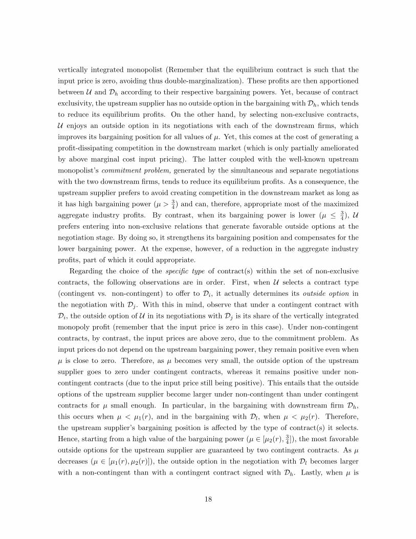
(iv) an exclusive contract to downstream firm Dh for µ ∈ [34 , 1].

Proof. See Appendix 4.

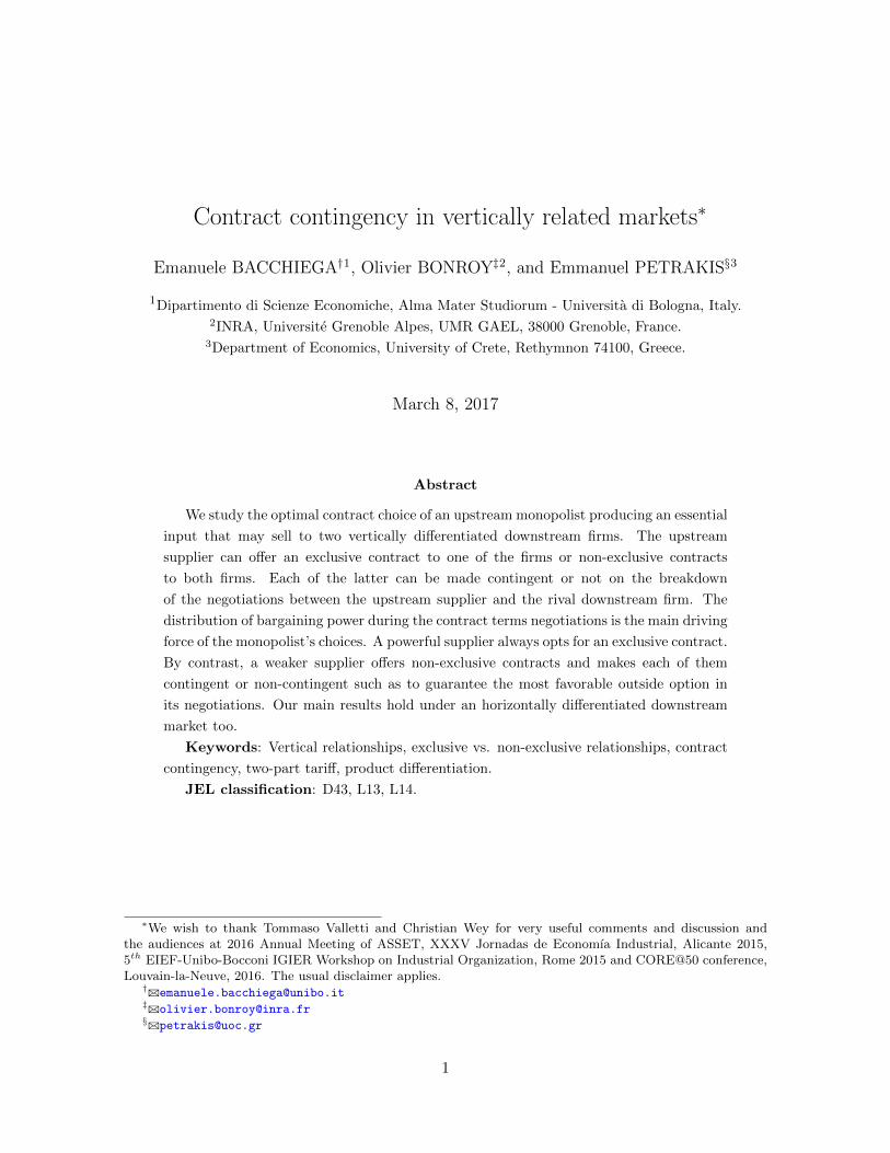
Figure 1 depicts in the (r, µ)-space the equilibrium contract selection. Two main mech-

anisms govern the choice of the upstream supplier over the type of contract(s) to be offered

to the downstream firms. The first mechanism concerns the choice between an exclusive con-

tract and two non-exclusive contracts. The second one applies to the choice within the class

of non-exclusive contracts and refers to the specific type of contract to be offered to each of

the downstream firms.

As far as the first trade-off is concerned, the forces at stake are as follows. On the

one hand, an exclusive contract allows U to create a monopoly in the downstream market.

As a consequence, aggregate industry profits are maximized and are equal to those of a

16

Exclusive contract

Contingent contracts

Contingent contract for firml

Non-contingent for firm h

Non-contingent contracts

0.0 0.2 0.4 0.6 0.8 1.0

0.0

0.2

0.4

0.6

0.8

1.0

μ

r

Figure 1: Equilibrium contract partition under price competition.

17

vertically integrated monopolist (Remember that the equilibrium contract is such that the

input price is zero, avoiding thus double-marginalization). These profits are then apportioned

between U and Dh according to their respective bargaining powers. Yet, because of contract

exclusivity, the upstream supplier has no outside option in the bargaining withDh, which tends

to reduce its equilibrium profits. On the other hand, by selecting non-exclusive contracts,

U enjoys an outside option in its negotiations with each of the downstream firms, which

improves its bargaining position for all values of µ. Yet, this comes at the cost of generating a

profit-dissipating competition in the downstream market (which is only partially ameliorated

by above marginal cost input pricing). The latter coupled with the well-known upstream

monopolist’s commitment problem, generated by the simultaneous and separate negotiations

with the two downstream firms, tends to reduce its equilibrium profits. As a consequence, the

upstream supplier prefers to avoid creating competition in the downstream market as long as

it has high bargaining power (µ > 34) and can, therefore, appropriate most of the maximized

aggregate industry profits. By contrast, when its bargaining power is lower (µ ≤ 34), U

prefers entering into non-exclusive relations that generate favorable outside options at the

negotiation stage. By doing so, it strengthens its bargaining position and compensates for the

lower bargaining power. At the expense, however, of a reduction in the aggregate industry

profits, part of which it could appropriate.

Regarding the choice of the specific type of contract(s) within the set of non-exclusive

contracts, the following observations are in order. First, when U selects a contract type

(contingent vs. non-contingent) to offer to Di, it actually determines its outside option in

the negotiation with Dj . With this in mind, observe that under a contingent contract with

Di, the outside option of U in its negotiations with Dj is its share of the vertically integrated

monopoly profit (remember that the input price is zero in this case). Under non-contingent

contracts, by contrast, the input prices are above zero, due to the commitment problem. As

input prices do not depend on the upstream bargaining power, they remain positive even when

µ is close to zero. Therefore, as µ becomes very small, the outside option of the upstream

supplier goes to zero under contingent contracts, whereas it remains positive under non-

contingent contracts (due to the input price still being positive). This entails that the outside

options of the upstream supplier become larger under non-contingent than under contingent

contracts for µ small enough. In particular, in the bargaining with downstream firm Dh,

this occurs when µ < µ1(r), and in the bargaining with Dl, when µ < µ2(r). Therefore,

the upstream supplier’s bargaining position is affected by the type of contract(s) it selects.

Hence, starting from a high value of the bargaining power (µ ∈ [µ2(r),34 ]), the most favorable

outside options for the upstream supplier are guaranteed by two contingent contracts. As µ

decreases (µ ∈ [µ1(r), µ2(r)]), the outside option in the negotiation with Dl becomes larger

with a non-contingent than with a contingent contract signed with Dh. Lastly, when µ is

18

small (µ ∈ [0, µ1(r)]), also the outside option in the negotiation with Dh becomes larger under

a non-contingent contract. The latter sheds light on why the upstream supplier never finds it

optimal to offer a contingent contract to Dh and a non-contingent contract to Dl.

5 Discussion of equilibrium outcomes

We should stress again that equilibrium input prices do not depend on the contingency or not

of the non-exclusive contracts. This is not surprising, because the variable part of the two-

tariff contract wi maximizes the excess joint profits of the (U ,Di) negotiating pair, whereas

the fixed part ti apportions the maximized excess joint profits to each of the involved parties

according to their respective bargaining powers. As a result, input prices are independent

of the distribution of the bargaining power. Note however that equilibrium input prices are

higher than the upstream marginal cost because of the upstream monopolist’s endeavor to

relax downstream price competition. Yet, the upstream monopolist is unable to publicly

commit to contracts and due to this commitment problem (O’Brien and Shaffer, 1992), the

equilibrium contract terms fail to maximize the aggregate industry profits.

As equilibrium input prices coincide under all types of non-exclusive contracts, the final

goods prices are the same as well. This, in turn, entails that equilibrium demands and

consumer surplus are the same too (compare Lemmata 2, 3 and 4). By contrast, the profits

accruing to the upstream supplier and the downstream firms differ, because the equilibrium

fixed fees are different under contingent, non-contingent and mixed contracts, reflecting the

differences in the upstream monopolist’s outside options.

Interestingly, the fixed fees may be positive or negative depending on the distribution of the

bargaining power, as reported in the following Lemma. Letting Ril ≡ wilDil + til, i ∈ {C,M,N}

be the upstream supplier’s profits from selling input to the low-quality firm, we obtain the

following results.

Lemma 5. (i) If the optimal contracts are non-contingent (i.e., µ ∈ [0, µ1(r)]), then the

fixed fees, tNh and tNl , are both negative; moreover, RNl < 0.

(ii) If the optimal contracts are mixed (i.e., µ ∈ [µ1(r), µ2(r)]), then:

∀r > 0.448 ⇒ tMh < 0, otherwise tMh R 0⇔ µ R4 + r − r2 −

√16 + 8r − 31r2 + 8r3

(6r − r2)≡ µMh (r)

∀r > 0.202 ⇒ tMl < 0, otherwise tMl R 0⇔ µ R3r

2 + r≡ µMl (r)

∀r > 0.472 ⇒ RMl < 0, otherwise RMl R 0⇔ µ Rr

2 + r≡ µMR (r)

19

(iii) If the optimal contracts are contingent (i.e., µ ∈ [µ2(r), 3/4]), then:

tCh R 0 ⇔ µ R8− r −

√64− 64r + r2

8≡ µCh (r)

tCl R 0 ⇔ µ R6 + r −

√20− 20r + r2

8≡ µCl (r)

RCl R 0 ⇔ µ R3−√

5

4≡ µCR(r)

Figure 2 depicts the various regions described in Lemma 5. In the purple-shaded areas

the respective variables take positive values, whereas in the yellow-shaded areas they take

negative values.

Under all types of non-exclusive contracts, if the bargaining power of the upstream sup-

plier is large (µ high), the share of the excess joint profits of each negotiating pair accruing,

via the fixed fee, to the upstream supplier is large. As µ decreases, the fixed fees shrink.

Ultimately, when µ becomes sufficiently small, the fixed fees become negative: The upstream

monopolist partially subsidizes, through the fixed fees, the downstream firms, yet it receives

positive payments via sales at input prices above its marginal cost. Surprisingly, the non-

exclusive contract offered to the low-quality downstream firm can, in fact, generate losses

for the upstream supplier, i.e., the positive revenues from input sales can be lower than the

negative fixed fee (see yellow region in Figure 2c).17 In this case, the upstream supplier op-

timally suffers such a loss in order to gain a stronger outside option in the negotiations with

the high-quality downstream firm that sells the “high value-added” product. The above are

particularly relevant under non-contingent contracts in which case both fixed fees tNh and tNlare always negative and at the same time, the revenue collected by input sales to Dl does not

cover the negative fixed fee - transfer downstream (i.e., RNl < 0).

The following Proposition summarizes our findings.

Proposition 2. Under non-contingent, non-exclusive equilibrium contracts, the fixed fees

always act as subsidies to the downstream firms, and moreover, the contract offered to the low-

quality downstream firm generates a loss for the upstream supplier. These observations hold

also under contingent and mixed, non-exclusive equilibrium contracts as long as the bargaining

power of the upstream supplier is sufficiently low.

Note that the parameter space in which fixed fees are negative grows larger as the products

become less differentiated (as r increases). Intuitively, the less differentiated the products,

the smaller the industry producer surplus to be shared among the upstream supplier and

the downstream firms. As downstream firms pay positive input prices, but should still earn

17Note that for any µ we have Rih = wihDih + tih > 0, i.e., the contract offered to the high-quality firm

generates always gains for the upstream supplier.

20

tNh<0

tCh<0

tCh>0

tMh<0

tMh>0

0.0 0.2 0.4 0.6 0.8 1.0

0.0

0.2

0.4

0.6

0.8

1.0

r

μ

(a) tCh , tMh

tNl<0

tCl<0

tCl>0

tMl<0

tMl>0

0.0 0.2 0.4 0.6 0.8 1.0

0.0

0.2

0.4

0.6

0.8

1.0

r

μ

(b) tCl , tMl

RNl<0

RCl<0

RCl>0

RMl<0

RMl>0

0.0 0.2 0.4 0.6 0.8 1.0

0.0

0.2

0.4

0.6

0.8

1.0

r

μ

(c) RCl , RM

l

Figure 2: Optimal tariffs and total profit from Dl under Contingent and Mixed equilibriumcontracts.

overall non-negative profits, a higher part of the industry producer surplus accrues to them

as the goods become less differentiated.

6 Extensions

6.1 Quantity competition

In this Section, we explore the optimal choice of contracts by the upstream supplier under

the alternative assumption of downstream quantity competition. It is well-known that com-

petition in quantities softens the competitive pressure on firms in one-tier industries (see e.g.

Singh and Vives, 1984), but this result is not robust when considering multi-layer industries

(Alipranti et al., 2014). As most of the analysis parallels that of downstream price competi-

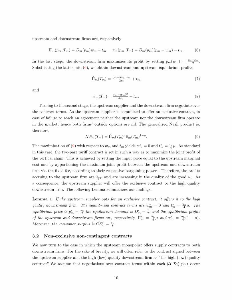
tion, we report hereafter only our main findings.18 Figure 3 depicts the equilibrium contract

configurations in the (r, µ) space of parameters.

The main message drawn from Figure 3 is that, under downstream quantity competition,

the equilibrium contract selection conveys important similarities to the case of price competi-

tion considered above. In particular, when U has relatively high bargaining power, it selects

to enter into an exclusive relationship with Dh. For intermediate values of the bargaining

power, U offers two non-exclusive, contingent contracts. Whereas for lower values of µ, Uoffers a contingent contract to Dl and a non-contingent one to Dh. These contract offers are

qualitatively similar to the case of downstream price competition. Yet, in contrast to price

competition, U never offers non-contingent contracts to both downstream firms.

18Needless to say, the detailed analysis, which follows exactly the same steps as under downstream pricecompetition, is available upon request.

21

Exclusive contract

Contingent contracts

Contingent contract for firm l ,

non-contingent for firm h

0.0 0.2 0.4 0.6 0.8 1.0

0.0

0.2

0.4

0.6

0.8

1.0

r

μ

Figure 3: Equilibrium contract partition under quantity competition.

A few observations are worth making here, that will help in pinpointing the similarities

and divergences relative to the downstream price competition case. First, under exclusive

contracts there is no competition downstream and the equilibrium outcome is as in Section

3.1. Second, equilibrium input prices again coincide under different non-exclusive contract

configurations, yet they are now below upstream marginal cost due to the commitment prob-

lem (see, e.g. Alipranti et al., 2014). The latter tends to reduce, relative to the downstream

price competition case, the profits accruing to the upstream supplier.

An immediate consequence is that non-contingent contracts offered to both downstream

firms are never optimal for the upstream supplier. In fact, when µ is low, the fixed fees

ti, i = h, l are small. In addition, the upstream supplier’s outside options under non-contingent

contracts are negative. As a consequence, U ’s profits are small and eventually become negative

for low enough µ (and are thus significantly lower than in the case of downstream price

competition). By contrast, a contingent contract offered to Dl, along with a non-contingent

one offered to Dh, makes the outside option of U in its bargaining with Dl positive and as a

consequence, the mixed contract configuration dominates non-contingent contacts offered to

both downstream firms.

The intuition regarding the upstream supplier’s choice between an exclusive contract of-

22

fered to Dh and non-exclusive, contingent contracts offered to both downstream firms is

qualitatively similar to that under downstream price competition. This is also the case for

the upstream supplier’s choice between the latter contracts and the mixed contracts.

The comparison of the regions in which mixed contracts are selected - the green areas in

Figures 1 and 3 - leads to a last remark. Contrary to the case of downstream price com-

petition, mixed contracts under quantity competition are never optimal when the degree of

vertical product differentiation is low (large r).19 In the latter case downstream competition

is fierce and as a consequence, the total producer surplus generated in the industry is small,

entailing that U ’s outside options are small too. This implies that under mixed contracts, as

the products become more homogeneous, the outside option of U in the negotiation with Dl

becomes small (and eventually negative) even for relatively large values of µ. By contrast,

under contingent contracts, the upstream supplier’s outside options, albeit lower under down-

stream quantity competition, are non-negative even when the degree of product differentiation

is small. As a consequence, U opts to offer contingent contracts to both downstream firms in

this case.

6.2 Alternative utility specification

One natural question that may arise is to which extent our results rely on the assump-

tion of vertically differentiated products with Mussa and Rosen (1978) utility function (MU,

henceforth). In this section, we demonstrate that qualitatively similar results hold when

the products are horizontally differentiated and the utility function is as specified in Bowley

(1924), Spence (1976) and Dixit (1979) (BSD, henceforth). In particular, the utility of the

representative consumer is

U(D1, D2) = αD1 + αD2 −1

2

(D2

1 +D22 + 2γD1D2

)+m, (28)

where Di is the quantity of good i, i ∈ {1, 2} that the consumer purchases and m is the

respective quantity of the “composite” good. The consumer’s optimal behavior gives rise to

the following linear demand system

D1(p1, p2) =α(1− γ)− p1 + γp2

1− γ2, D2(p1, p2) =

α(1− γ)− p2 + γp11− γ2

, (29)

where p1 and p2 are the prices of goods 1 and 2 respectively, α > 0 and γ ∈ (0, 1) indicates the

degree of product substitutability. When γ is close to zero, the goods are almost independent,

whereas when γ tends to one, the goods become almost homogenous. The most remarkable

19Indeed, in order mixed contracts to be optimal, a necessary (but not sufficient) condition is that r < 0.382,see figure 3.

23

0.0 0.2 0.4 0.6 0.8 1.0

0.0

0.2

0.4

0.6

0.8

1.0

γ

μ

Exclusive

contract

Contingent contracts

Non-contingent contracts

(a) Price competition

0.0 0.2 0.4 0.6 0.8 1.0

0.0

0.2

0.4

0.6

0.8

1.0

γμ

Exclusive contract

Contingent contracts

(b) Quantity competition

Figure 4: Equilibrium contract configurations with BSD utility.

differences between the present model and our main model are that under the utility function

in (28) (i) the goods are symmetric from the point of view of the consumer and (ii) the

consumer is not restricted to purchase discrete quantities of the goods.

The analysis here closely follows the steps presented in the previous sections. To save

on space, we will present the main findings under the BSD utility specification diagrammat-

ically.20 Figure 4, panel (4a) and panel (4b), depict the equilibrium contract configurations

under downstream price and quantity competition, respectively.

As can easily be seen from Figure 4, our findings under the BSD utility specification convey

important similarities with those under the MR utility specification. The most remarkable

difference is that the upstream supplier never finds it optimal to offer mixed contracts. In

contrast to the MR utility specification, as the consumer’s preferences are symmetric over the

two goods in this case, the upstream supplier is indifferent between offering the contingent

contract to downstream firm 1 (D1) and the non-contingent to downstream firm 2 (D2) or

vice versa. Mixed contracts are then dominated either by contingent or by non-contingent

contracts offered to both downstream firms. In particular, under quantity competition, mixed

contracts are always dominated by two contingent contracts, whereas under price competition

they are dominated by two contingent (non-contingent) contracts as long as µ is high (low).21

20The detailed analysis is available upon request.21The critical value is µ(γ) ≡ 2γ2(2−γ−γ2)

8+γ(1+γ)(2−γ2) which separates the regions of contingent and non-contingent

contracts in Figure 4 panel (4a).

24

Clearly, under quantity competition, a non-contingent contract signed with Di leads to an

outside option for the upstream supplier in its bargaining with Dj smaller than when it signs

a contingent contract with Di. As a result, two contingent contracts always dominate a mixed

contract. Under price competition, for low µ, U ’s outside option in the bargaining with Djunder a contingent contract signed with Di is smaller than when it signs a non-contingent

contract with Di. As a result, two non-contingent contracts dominate mixed contracts for

low values of µ. The reverse reasoning holds for high µ and thus, two contingent contracts

dominate mixed contracts.

Another difference lies in the characteristics of the parameter region in which an exclusive

contract is chosen by the upstream supplier. In fact, in the MR utility specification case,

under both price and quantity downstream competition, an exclusive contract is offered to

Dh for any degree of vertical product differentiation (provided that µ is large enough). This

is not so with the BSD utility specification, in which case an exclusive contract is offered

only if goods are close enough substitutes (γ high enough). This can be seen by comparing

Figures (1) and (3), with (4). This is due to the different nature of the two models. Under the

MR utility specification, the goods are vertically differentiated, with all consumers a priori

preferring the high-quality over the low-quality good. The coexistence of high- and low-

quality variants has a profit erosion effect that is particularly detrimental on the upstream

supplier’s revenues from the sales of the high-quality good, i.e., the good that allows for a

higher extraction of consumer surplus. As a consequence, when the upstream supplier can

extract most of the surplus from the downstream market (µ is high), it prefers to avoid

profit-dissipating downstream competition and opts thus for an exclusive contract with the

high-quality downstream firm. Under the BSD utility specification, goods are symmetrically

horizontally differentiated, with the representative consumer having a priori no preference

for one or the other good. As a consequence, when the degree of product substitutability

is low (γ is low), the loss in industry producer surplus due to downstream competition is

small. This entails that the upstream supplier prefers to strengthen its bargaining position by

offering non-exclusive, contingent contracts to both downstream firms even if it can extract

most of the industry producer surplus (µ high). By contrast, an exclusive contract becomes

rentable only if the degree of product substitutability is high. When γ is high, downstream

competition has a strong negative effect on industry producer surplus. Then the upstream

supplier prefers to avoid profit-eroding downstream competition, opting thus for an exclusive

contract.

25

7 Conclusion

We have investigated the optimal contract choice of an upstream monopolist that may sell an

essential input to two downstream firms that produce vertically differentiated products and

compete in prices or in quantities in the final goods market. In the outset of the game, the

upstream supplier can offer an exclusive contract to one of the downstream firms, or non-

exclusive contracts to both of them, in which case each of the contracts could be contingent

or non-contingent. Contract terms negotiations, and in particular over two-part tariffs, are

then conducted between the upstream supplier and the downstream firm(s). A non-contingent

contract does not allow renegotiation of contract terms with a downstream firm in case that

the upstream supplier does not reach an agreement with the rival downstream firm. A con-

tingent contract instead allows for different contract terms in case of agreement and in case

of disagreement in the negotiations between the upstream supplier and the rival downstream

firm.

We show that the distribution of the bargaining power and the degree of vertical product

differentiation play a crucial role in determining the equilibrium outcome. In particular, when

the bargaining power of the upstream supplier is relatively high, it prefers to sign an exclusive

contract with the high-quality downstream firm. In this way, it avoids downstream compe-

tition that erodes aggregate industry profits and moreover, it extracts most of the producer

surplus generated by the ensuing vertically integrated market structure. For lower values of

bargaining power, the upstream supplier opts for non-exclusive contracts. In this way, the

upstream supplier generates outside options in its negotiations with the downstream firms,

at the cost however of increasing downstream competition. By strengthening its bargaining

position, it obtains a larger share of an otherwise smaller industry producer surplus and in-

creases thus its profits. Further, we show that for intermediate bargaining power values, the

upstream supplier prefers to offer contingent contracts to both downstream firms; whereas for

lower values, it opts for mixed contracts, i.e., a contingent contract to the low-quality down-

stream firm and a non-contingent to the high-quality one. Finally, the upstream supplier offers

non-contingent contracts to both downstream firms only if the upstream bargaining power

is quite low and downstream firms compete in prices. This never occurs under downstream

quantity competition because the upstream monopolist suffers from a strong commitment

problem that results to negative input prices.

Finally, we have shown that our main findings are qualitatively similar when we consider

symmetrically horizontally differentiated markets. In those markets, if we replace the degree

of vertical product differentiation with the degree of product substitutability, we obtain a

similar partition of the parameter space regarding the upstream supplier’s contract choices.

Our analysis leads to a number of testable implications. In markets with a powerful

26

upstream supplier, we should observe foreclosure in the downstream market. In particular,

low-quality downstream firms are expected to be foreclosed by the upstream monopolist. By

contrast, when the upstream supplier is not so powerful, we should observe non-exclusive

contracts offered to downstream firms. In addition, the “complexity” of non-exclusive con-

tracts is expected to be positively related to the bargaining power of the upstream supplier:

More powerful suppliers should sign contracts including clauses that allow for renegotiation in

case of an increase in downstream concentration, whereas in contracts signed by less powerful

upstream suppliers, such clauses are expected to be absent. Furthermore, mixed contracts

should mainly be observed in markets where goods dispose some vertical product differenti-

ation characteristics, whereas they should be much less common in markets for horizontally

differentiated goods. Finally, in markets with quantity competition, exclusive contracts should

be observed more frequently than in markets characterized by price competition.

Our analysis suggests several lines for future research. First, one direction is to consider

that the two downstream firms have different bargaining powers relative to the upstream

supplier. We expect that our intuitive arguments concerning the choice between exclusive

and non-exclusive contracts would apply in this case too. However, due to the asymmetry

in bargaining powers, mixed contracts with a contingent contract offered to high-quality firm

and a non-contingent to the low-quality firm could emerge. Another direction is to let the

number of competing downstream firms increase. The configuration of contracts to be offered

by the upstream supplier is expected to be richer now, but the upstream bargaining power

will still play a significant role in its choice of specific contracts. One should expect that the

higher the upstream bargaining power, the more concentrated the downstream market will

be.

References

Acharyya, R. (1998). “Monopoly and product quality: Separating or pooling menu?” Eco-

nomics Letters, 61(2):187–194.

Alipranti, M., Milliou, C., and Petrakis, E. (2014). “Price vs. quantity competition in a

vertically related market”. Economics Letters, 124(1):122–126.

Bacchiega, E., Bonroy, O., and Mabrouk, R. (2013). “Paying not to sell”. Economics Letters,

121(1):137–140.

Bazerman, M. H. and Gillespie, J. J. (1998). “Betting on the future: the virtues of contingent

contracts.” Harvard Business Review, 77(5):155–60.

Bonnet, C. and Dubois, P. (2010). “Inference on vertical contracts between manufacturers and

27

retailers allowing for nonlinear pricing and resale price maintenance”. The RAND Journal

of Economics, 41(1):139–164.

Bowley, A. L. (1924). The mathematical groundwork of economics. Oxford University Press,

reprinted by A.M. Kelley New York, 1965.

Byialogorsky, E. and Gerstner, E. (2004). “Contingent Pricing to Reduce Price Risks”. Mar-

keting Science, 23(1):146–155.

Chambolle, C. and Villas-Boas, S. B. (2015). “Buyer power through the differentiation of

suppliers”. International Journal of Industrial Organization, 43:56–65.

de Fontenay, C. C. and Gans, J. S. (2005). “Vertical Integration in the Presence of Upstream

Competition”. RAND Journal of Economics, pages 544–572.

Dixit, A. K. (1979). “A model of duopoly suggesting a theory of entry barriers”. The Bell

Journal of Economics, 10(1):20–32.

European Commission (1999). “Buyer Power and its Impact on Competition in the Food Re-

tail Distribution Sector of the European Union”. Technical report, European Commission,

DG IV, Brussels.

FTC (2001). “Report on the Federal Trade Commission Workshop on Slotting Allowances

and Other Marketing Practices in the Grocery Industry”. Technical report, Federal Trade

Commission, Washington D.C.

Gabszewicz, J. J. and Thisse, J.-F. (1979). “Price competition, quality and income dispari-

ties”. Journal of Economic Theory, 20(3):340–359.

Hart, O. and Holmstrom, B. (1987). “The Theory of Contracts”. In T. Bewley, editor,

“Advances in Economic Theory, 5th World Congress of the Econometric Society”, pages

71–155.

Hart, O. and Tirole, J. (1990). “Vertical Integration and Market Foreclosure”. Brookings

Papers on Economic Activity. Microeconomics, pages 205–286.

Horn, H. and Wolinsky, A. (1988). “Bilateral Monopolies and Incentives for Merger”. The

RAND Journal of Economics, 19(3):pp. 408–419.

Inderst, R. and Mazzarotto, N. (2008). “Buyer Power in Distribution”. In W. Collins, editor,

“Issues in Competition Law and Policy”, (ABA Antitrust Section Handbook), pages 1953–

1978. ABA.

28

Inderst, R. and Wey, C. (2003). “Bargaining, Mergers, and Technology Choice in Bilaterally

Oligopolistic Industries”. RAND Journal of Economics, pages 1–19.

Inderst, R. and Wey, C. (2007). “Buyer power and supplier incentives”. European Economic

Review, 51(3):647–667.

Iozzi, A. and Valletti, T. (2014). “Vertical bargaining and countervailing power”. American

Economic Journal: Microeconomics, 6(3):106–135.

Law, J., editor (2016). A Dictionary of Law. Oxford University Press, online (8th) edition.

Marx, L. M. and Shaffer, G. (2010). “Slotting Allowances and Scarce Shelf Space”. Journal

of Economics & Management Strategy, 19(3):575–603.

McAfee, R. P. and Schwartz, M. (1994). “Opportunism in Multilateral Vertical Contract-

ing: Nondiscrimination, Exclusivity, and Uniformity”. The American Economic Review,

84(1):pp. 210–230.

McAfee, R. P. and Schwartz, M. (1995). “The non-existence of pairwise-proof equilibrium”.

Economics Letters, 49(3):251–259.

Miklos-Thal, J., Rey, P., and Verge, T. (2011). “Buyer power and intrabrand coordination”.

Journal of the European Economic Association, 9(4):721–741.

Milliou, C. and Petrakis, E. (2007). “Upstream horizontal mergers, vertical contracts, and

bargaining”. International Journal of Industrial Organization, 25(5):963–987.

Mussa, M. and Rosen, S. (1978). “Monopoly and Product Quality”. Journal of Economic

Theory, 18(2):301–317.

O’Brien, D. P. and Shaffer, G. (1992). “Vertical Control with Bilateral Contracts”. The

RAND Journal of Economics, 23(3):pp. 299–308.

OECD (1999). “Buying Power of Multiproduct Retailers”. Technical report, Series Roundta-

bles on Competition Policy DAFFE/CLP(99)21. OECD, Paris.

Rey, P. and Tirole, J. (2007). “Chapter 33 A Primer on Foreclosure”. volume 3 of Handbook

of Industrial Organization, pages 2145–2220. Elsevier.

Rey, P. and Verge, T. (2004). “Bilateral Control with Vertical Contracts”. The RAND Journal

of Economics, 35(4):pp. 728–746.

Shaffer, G. (1991). “Slotting Allowances and Resale Price Maintenance: A Comparison of

Facilitating Practices”. The RAND Journal of Economics, 22(1):120–135.

29

Shaked, A. and Sutton, J. (1983). “Natural oligopolies”. Econometrica, 51(5):1469–1483.

Singh, N. and Vives, X. (1984). “Price and Quantity Competition in a Differentiated

Duopoly”. The RAND Journal of Economics, 15(4):546–554.

Spence, M. (1976). “Product Differentiation and Welfare”. American Economic Review,

66(2):407–14.

Thanassoulis, J. and Smith, H. (2009). “Bargaining between retailers and their suppliers”. In

A. Ezrachi and U. Bernitz, editors, “Private Labels, Brands and Competition Policy: The

Changing Landscape of Retail Competition”, Oxford University Press.

Villas-Boas, S. B. (2007). “Vertical relationships between manufacturers and retailers: Infer-

ence with limited data”. The Review of Economic Studies, 74(2):625–652.

Appendix

1 Contingent contracts: the case 34 < µ ≤ 1

Assume that 34 < µ ≤ 1. In this parameter region the low-quality downstream firm cannot

enjoy non-negative profits in the interior solution, nonetheless, to sign the contract, it must

not incur losses as well. As a consequence, the equilibrium contract must be such that the

low quality downstream firm reaps zero profits. Nevertheless, the low quality contract must

still maximize the excess joint profits of the (U ,Dl) pair which, by virtue of the foregoing

observation, completely accrue to the upstream supplier. In fact, the fixed fee charged by

U to Dl is adjusted downwards such that the downstream firm is indifferent between signing

or not the contract. Thus, the equilibrium contracts are obtained by solving the following

problem

maxwh,th

NPCh (Th, TCl ), max

wl[Π(TCh , Tl) + πl(Tl, w

Ch )], and πl(Tl, w

Ch )

tl= 0. (30)

The equilibrium contracts are then

TCh = (wCh , tCh ) =

(ul4,4uhµ+ ul(−3 + (3− 4µ)µ)

16

)(31)

TCl = (wCl , tCl ) =

(u2l

4uh,ul(uh − ul))

16uh

). (32)

The equilibrium prices are pCh = 2uh−ul4 , pCl = ul

4 , and the equilibrium demands are DCh =

30

12 , DC

l = 14 . The equilibrium profit of the upstream supplier is ΠC = µ[4uh+ul(3−4µ)]

16 < Π∗m.

Such a contract is then strictly dominated by an exclusive contract.

2 Contingent high-quality contract and non-contingent low-

quality contract

Let us consider the case in which U offers a contingent contract to Dh and a non-contingent

contract to Dl. Let TZi ≡ (wZi , tZi ), i = h, l be the equilibrium contracts. Using similar argu-

ments as in (3.3) to determine the outside options for the upstream supplier, the generalized

Nash products turn out to be

NPZh (Th, TZl ) =

[Π(Th, T

Zl )− Πm(TZl )

]µπh(Th, w

Zl )1−µ, (33)

NPZl (TZh , Tl) =[Π(TZh , Tl)−

uh4µ]µπl(Tl, w

Zh )1−µ. (34)

As in (3.3), (33) and (34) are locally concave at the solution of the focs only if µ ≤ 2u2h+2uhul−u2l4u2h+2uhul−u2l

(otherwise, NPZl (·) is no longer locally concave because D` makes negative profits.) If this

condition holds, standard maximization techniques lead to the following equilibrium contracts

TZh = (wZh , tZh ) =

(ul4,8µu3h − 4(1 + µ)u2hul + 2(1− µ)uhu

2l − (1− µ)u3l

32u2h

), (35)

TZl = (wZl , tZl ) =

(u2l

4uh,ul{

2µ(3− 2µ)u2h + 2[(2− µ)µ− 2]uhul + (1− µ)2u2l}

32u2h

). (36)

Note that as the generalized Nash products NPZh (Th, TZl ) and NPNh (Th, T

Nl ) are similar and

do not depend on the fixed fee offered to Dl, then TZh = TNh . Then the equilibrium final good

prices are pZh = 2uh−ul4 , pZl = ul

4 , and the equilibrium demands are DZh = 1

2 , DZl = 1

4 . The

equilibrium profits of the upstream supplier is ΠZ =µ[8u3h+(2−4µ)u2hul−2(µ−1)uhu

2l+(µ−1)u3l ]

32u2h.

If µ >2u2h+2uhul−u2l4u2h+2uhul−u2l

, the upstream supplier should adjust downwards the fixed fee in order

to incentivize the low quality firm to sign the contract. Then the optimal contracts are the

solution to

maxwh,th

NPZh (Th, TZl ), max

wl[Π(TZh , Tl) + πl(w

Zh , Tl)], and πl(w

Zh , Tl)

tl= 0. (37)

31

Standard maximization techniques then lead to the optimal contracts

TZh = (wZh , tZh ) =

(ul4,8µu3h − 4(1 + µ)u2hul + 2(1− µ)uhu

2l − (1− µ)u3l

32u2h

), (38)

TZl = (wZl , tZl ) =

(u2l

4uh,ul(uh − ul)

16uh

). (39)

The equilibrium final good prices and demands are as above, while the equilibrium profits of

the upstream supplier is ΠZ =ul(2u2h+2uhul−u2l )+µ(2uh+ul)(2uh−ul)

2

32u2h.

Note that as ΠZ < ΠC , a non-contingent contract offered to Dl and a contingent contract

to Dh is strictly dominated by the upstream supplier offering contingent contracts to both

firms.

3 Proof of Lemma 4 part ii)

If U offers a contingent contract to Dl and a non-contingent contract to Dh and moreover,uluh

> 45 and

8u2h−4uhul−u2l

ul(6uh−ul) < µ < 1, in the interior solution the high-quality downstream

firm makes negative profits. The upstream supplier should adjust the fixed fee downwards in

order to incentivize Dh to sign the contract. Equilibrium contracts is then the solution to the

following problem

maxwl,tl

NPMl (TMh , Tl), maxwh

[Π(Th, TMl ) + πh(Th, w

Ml )], and πh(Th, w

Ml )

th= 0. (40)

Thus, the equilibrium contracts are

TMh = (wMh , tMh ) =

(ul4,uh − ul

4

), (41)

TMl = (wMl , tMl ) =

(u2l

4uh,ul[2µuh − (3− µ)ul]

32uh

). (42)

The equilibrium prices are pMh = 2uh−ul4 , pMl = ul

4 , and the equilibrium demands are DMh = 1

2 ,

DMl = 1

4 . The equilibrium profit of the upstream supplier is ΠM =8u2h−2(2−µ)uhul−(1−µ)u

2l

32uh<

Π∗m. Hence, this pair of contracts is strictly dominated by an exclusive contract offered to the

high-quality firm.

4 Proof of Proposition 1

As we have seen above, some contract configurations are strictly dominated strategies for the

upstream supplier. This is so for those contracts in which the upstream supplier should adjust

32

the fixed fee downwards to motivate the high, or the low, quality downstream firm to sign the

contract. These contracts are strictly dominated by an exclusive contract offered to Dh (see

Appendix 1 and 3). In addition, a non-contingent contract offered to Dl and a contingent

contract to Dh is also strictly dominated strategy by contingent contracts offered to both

downstream firms (see Appendix 2).

After the elimination of strictly dominated strategies, we determine the optimal contracts

for the upstream supplier in the first stage by simply comparing its profits at the equilibria

of each subgame

(i) if µ ∈ [0, µ1(r)), then ΠN > max[Π∗m, ΠM , ΠC ],

(ii) if µ ∈ [µ1(r), µ2(r)), then ΠM > max[Π∗m, ΠN , ΠC ],

(iii) if µ ∈ [µ2(r),34), then ΠC > max[Π∗m, ΠN , ΠM ],

(iv) if µ ∈ [34 , 1], then Π∗m > max[ΠC , ΠN , ΠM ],

with r ≡ uluh

, µ1(r) ≡ r(1−r)(6−r) , µ2(r) ≡ 2(1−r)

6−r , and 0 < µ1(r) < µ2(r) <3

4.

33