Contour current driven continental slope-situated sandwaves with effects from secondary current processes on the Barents Sea margin offshore Norway

Marine Geology 353 (2014) 108–127

Contents lists available at ScienceDirect

Marine Geology

j ourna l homepage: www.e lsev ie r .com/ locate /margeo

Contour current driven continental slope-situated sandwaves witheffects from secondary current processes on the Barents Sea marginoffshore Norway

Edward L. King a, Reidulv Bøe b, Valérie K. Bellec b, Leif Rise b, Jofrid Skarðhamar c,Bénédicte Ferré d, Margaret F.J. Dolan b

a Geological Survey of Canada-Atlantic (GSC-A), 1 Challenger Drive, P.O. Box 1006, Dartmouth, Nova Scotia B2Y 4A2, Canadab Geological Survey of Norway (NGU), P.O. Box 6315 Sluppen, N-7491 Trondheim, Norwayc Institute of Marine Research (IMR), P.O. Box 6404, N-9294 Tromsø, Norwayd CAGE—Centre for Arctic Gas Hydrate, Environment and Climate, Department of Geology, University of Tromsø (UiT), NO-9037 Tromsø, Norway

E-mail addresses: [email protected] (E.L. King), [email protected] (J. Skarðhamar), [email protected]

http://dx.doi.org/10.1016/j.margeo.2014.04.0030025-3227/Crown Copyright © 2014 Published by Elsevie

a b s t r a c t
a r t i c l e i n f o
Article history:Received 27 March 2013Received in revised form 3 April 2014Accepted 6 April 2014Available online 15 April 2014

Communicated by J.T. Wells

Keywords:sandwave morphometricssubaqueous dunesand transportNorwegian Atlantic Currentcontour currentdeep Ekman effectinternal waveglacigenic debris flow

Seabed data acquired from the southern Barents Sea continental margin offshore Norway reveal detailed mor-phology of large sandwave fields. Multibeam echosounder bathymetry and backscatter, shallow seismic, sedi-ment samples and seabed video data collected by the MAREANO program have been used to describe andinterpret the morphology, distribution and transport of the sandwaves. The bedforms lie on a slope dominatedby relict glacial forms andmuddy/sandy/gravelly sediments. Sandwave migration across small gravity mass fail-ures of the glacial mud constrains the field initiation as early post glacial or later. The contour-parallel nature ofthe fields and crestlines normal to the bathymetry contours and the geostrophic Norwegian Atlantic Current(NwAC) demonstrate that the NNW-flowing oceanographic circulation is the primary driving current. The fieldscoincide with the depth range at which a transition betweenwarm, saline and underlying cooler, less saline wa-ters fluctuate across the seabed. Statistically rigorous measurements of height, width and various parameters ofslope and symmetry confirm a tendency to downstream (NNW) sandwavemigration butwith significant excep-tions. Anomalous bedform symmetry domains within the fields are tuned to meso-scale topography along(relict) glacial debris flow chutes, indicating current focusing. Upstream and upper slope-derived winnowedsand transport eroded from the glacial sediments is the supposed source. Sandwave flank slope values are com-parable to the regional slope such that the gravitational vector would have a cumulative downslope migrationaffect unless balancedbyupslope drivers. Perpendicular cross-cutting of stoss face 3-D ripples by linear (2-D) rip-ples in the sandwave troughs and lee faces is evidence for non-synchronous, episodic current variations. Thoughdeep Ekman transport and internal wave action are unproven here, these could explain chute-related tuning ofbedform symmetry through funneling in the debris flow chutes and favor sand recycling, thus contributing tolong-term maintenance of the sandwave field.

Crown Copyright © 2014 Published by Elsevier B.V. All rights reserved.

1. Introduction

The focus of this study is recently surveyed upper-slope situatedsandwave fields in the SW Barents Sea of the Norwegian continentalmargin. Sandwaves are indicative of strong currents that potentiallychallenge water column and seabed engineering operations. Their dy-namic nature poses challenges for seabed infrastructure such as pipe-lines and cables. While shelf-situated sandwaves are well documentedon a global scale, the nearest located on the adjacent shelf (Bøe et al.,2009), known occurrences of present-day slope-situated sandwavesunder a contour current influence are limited. These include examples

[email protected] (R. Bøe),it.no (B. Ferré).

r B.V. All rights reserved.

on the Canary Islands (Wynn et al., 2000), the South China Sea(Damuth, 1980; Reeder et al., 2011), the Strait of Gibraltar (Heezenand Hollister, 1971), Gulf of Cadiz (Kenyon and Belderson, 1973;Baraza et al., 1999; Habgood et al., 2003; Mulder, 2003; Hanquiezet al., 2007), and the Faeroe–Shetland Channel (Masson, 2001).Sandwaves in this study were first noted from sidescan investigationsby Kenyon (1986) who attributed them to poleward current and sug-gested the potential of sand transport to the deep sea through associat-ed channels.

Factors controlling deposition of continental shelf bottom-currentsands (by tidal, wave and geostrophic currents) include hydrodynamicregime (seconds to years time scale), availability of sandy sediments(accumulation, export and preservation potential) and physiographiccontext of the area swept by the currents (Viana et al., 1998a, 1998b).

http://crossmark.crossref.org/dialog/?doi=10.1016/j.margeo.2014.04.003&domain=pdf

http://dx.doi.org/10.1016/j.margeo.2014.04.003

mailto:[email protected]




http://dx.doi.org/10.1016/j.margeo.2014.04.003

http://www.sciencedirect.com/science/journal/00253227

109E.L. King et al. / Marine Geology 353 (2014) 108–127

All are modulated by a long-term (post-glacial) global sea-level and cli-mate regime. The slope-setting processes affecting sandwaves are morepoorly understood; those driven by contour currents are not well repre-sented in the literature. A summaryof deep-water sedimentwave formsby Wynn and Stow (2002) shows dominance of those classified as“bottom current waves” and “turbidity current waves”. The former aregenerally associated with contouritic drifts, are generally larger, alignedoblique to the contours, muddy, bioturbated, and have long-termgrowth and transport histories. The latter are normally associatedwith turbidite channels and levees, oftenwith crestlines parallel to con-tours, wavelengths changing downslope, and comprising amix of turbi-dites and hemipelagic sediments. The Barents Sea sandwave fieldscontrast in a uniformly sand composition, constant contour-normalcrestline orientation, relative independence of slope topographic per-turbations and relatively short-lived (post-glacial) history.

Following the terminology of Belderson et al. (1982) we use theterm sandwave to refer to the subaqueous, lower flow regime, trans-verse bedforms of sand that have wavelengths larger than sand ripples.Where two ormore sizes of sandwaves occur together or superimposedit is convenient to refer to them as small sandwaves (identical to dunesor megaripples; see discussions in Allen, 1980; Amos and King, 1984;Ashley, 1990) and large sandwaves, without implying any geneticdifference in the terminology. This is because there appears to be acomplete gradation in size, plan view and lee slope angle betweensandwaves at various locations (Belderson et al., 1982). In our studyarea the driving current is generally from SSE to NNW, along theTromsøflaket slope, and the southern bedform face is referred to asstoss and the northern as lee except where noted.

The ultimate aim of the ongoing sandwave study is to elucidate gov-ernors of process, sand source, age of the bedform field and presentmo-bility. Initial results of the sandwave study are reported in King et al.(2011). The focus here is to evaluate MAREANO's (www.mareano.no)geological and geophysical data including multibeam bathymetry andbackscatter, shallow seismic, videos and seabed samples, and initialoceanographic (conductivity, temperature, depth, CTD) measurements.We examine the general oceanographic setting, the geomorphology offeatures such as slope channels, slide scars and glacial debris flowswith-in a sand sink-source context, make inferences from a rigorous dataset

N o

r w

a y

S w

e d

e n

NorwegianSea

NorwegianSea

sandwave fieldssandwave fields

Trom

Bjørnøya TrouBjørnøya(Bear Island)

trough-mouth fan

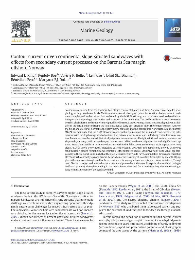
Fig. 1. Location of the sandwave study area on the southwest Barents Sea continental slope. Redreader is referred to the web version of this article.)

of measurements (metrics) on the bedforms, and synthesize these tosuggest an origin and evolution of the sand and bedform fields andthe processes driving their formation and mobility.

To date no detailed studies on the SW Barents Sea slope sandwaveexamples have been conducted. Several fields are present on the slopeat a 600 to 800 m depth (Fig. 1). From the outset, the sandwave fields,lying in the path of the northern extension of the North Atlantic Currentwere recognized as probablemanifestations of the geostrophic currents.Further study of the geologic setting and sandwavemorphometric stud-ies was undertaken to determine if secondary influence(s) on thesandwaves was revealed, such as topographic focusing, channeled up-or down welling, or internal waves. Furthermore, their spatial coinci-dence with an oceanographic thermocline positioned them as candi-dates for influence by (unproven) internal or solitary waves.

2. Bathymetric and geologic setting

The sandwave fields are located on the continental slope in the tran-sition zone between the Norwegian Sea in thewest and the Barents Seain the east. The southern Barents Sea continental shelf comprises alter-nating shallow banks and deeper troughs formed during the last glacia-tions (Figs. 1 and 2), andmassive diamictic sediments are found (Vorrenet al., 1984; Ottesen et al., 2005; Andreassen et al., 2008; Winsborrowet al., 2010). The bank adjacent to the sandwaves in the south,Tromsøflaket, is characterized by N–S-trending, very long and elevatedmoraines. The sandwave fields are only 1–3 km from the 400 m deepshelf break off Tromsøflaket, but this increases to 6 km in the north.

The Bear Island Trough cuts across the Barents Sea shelf north of thesandwave area, with water depths of 300–400 m, transitioning to theBear Island Trough Mouth Fan (Fig. 1) in the west (Laberg and Vorren,1995). At the shelf break, the 100m high escarpments (Fig. 2) of the gi-gantic 200,000–300,000 year old Bear Island Slide occur (Laberg andVorren, 1993).

MAREANO data and data from earlier studies show a surficial sedi-mentation pattern on the continental shelf influenced by pre-existingglacial features and sediments, bathymetry and ocean currents (e.g.,Hald and Vorren, 1984; Vorren et al., 1984, 1989; Bellec et al., 2008;Bøe et al., 2009, 2010; Buhl-Mortensen et al., 2010). Lag deposits

0 50 100 km

Barents Sea

søflaket

gh

TromsøTromsø

areasmark sandwave fields. (For interpretation of the references to color in this figure, the

http://www.mareano.no

N1N2

N5 S1

N3&4

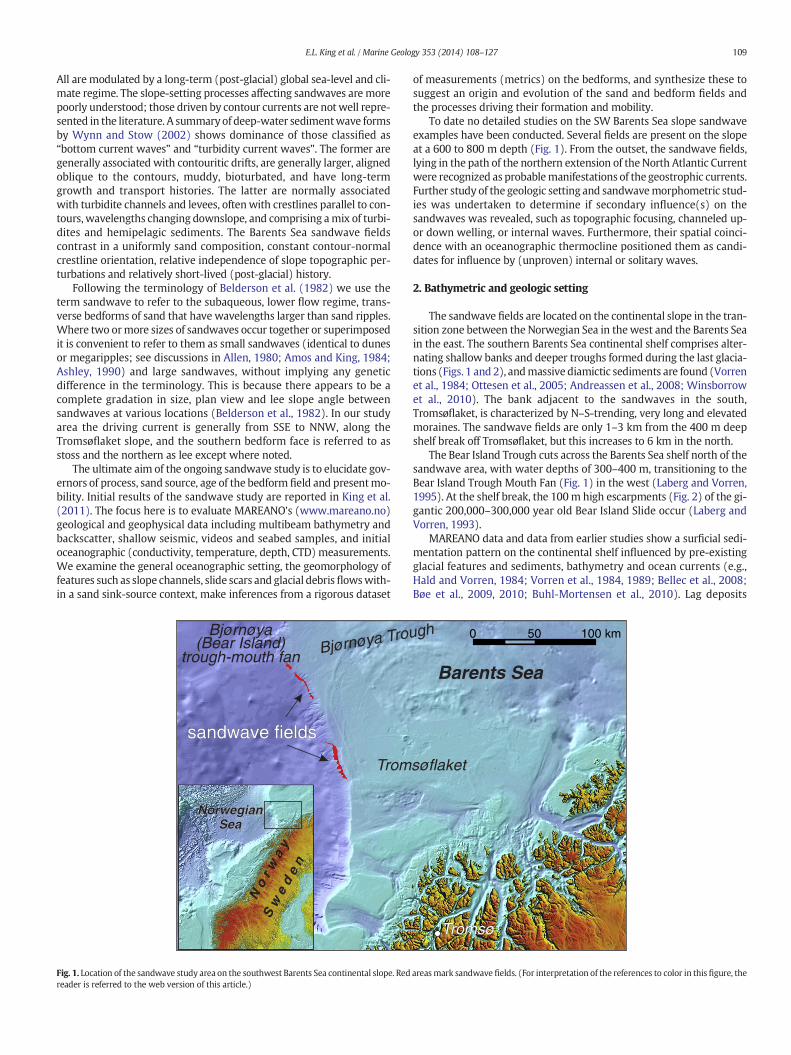
Fig. 2. 3-D rendering ofmultibeam sonar shaded relief bathymetry showing the general setting of the sandwave fields (dark gray, designated N1 to N5 and S1). These are situated below aglaciated and (relict) iceberg scoured shelf, south of the large Bear Island Slide, and superimposed onmultiple canyon-like chutesmainly from glacial processes. The bedforms range from480 to 750 m water depth. Bottom panel is a closer view and low-angle perspective of the S1 field.

110 E.L. King et al. / Marine Geology 353 (2014) 108–127

occur on banks and locally on the continental slope (Fig. 3), testifying tothe influence of a high-energy environment eroding the glacial sedi-ments. Deposition of fine-grained sediments occurs in troughs and shel-tered depressions (Vorren et al., 1984; Michels, 2000). The outermostshelf and just beyond the shelf breakhave little sand, with the exceptionof some partiallyfilled iceberg scour troughs.Winnowing by along slope(contour) currents of the upper slope has occurred during interglacialperiods (Laberg and Vorren, 1993, 1995). A contourite deposit compris-ing fine-grained sediments has been described below 1000 m depthsouth of the study area, on the slope off Lofoten (Laberg et al., 1999;Laberg and Vorren, 2004).

Glaciers advanced through fjords onto the continental shelf, locallydeveloped into ice streams and reached the shelf edge during the last(lateWeichselian) glaciation,which reached amaximum slightly before18,000 C14 BP. Deglaciation of deep troughs took place from ~15,000 C14

BP, but ice was grounded on the outer shelf banks for a longer period(Winsborrow et al., 2010). During the middle–late Pleistocene, debrisflow activity dominated the slope (Laberg and Vorren, 1995; Vorrenet al., 1998; Laberg et al., 2010). The debris flows have unique geometry,lithology and flow characteristics related to their shelf–break situatedice stream source and are termed glacigenic debris flows, abbreviatedGDFs (King et al., 1996; Nygård et al., 2002).

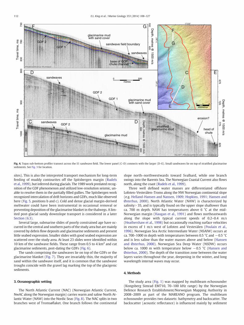
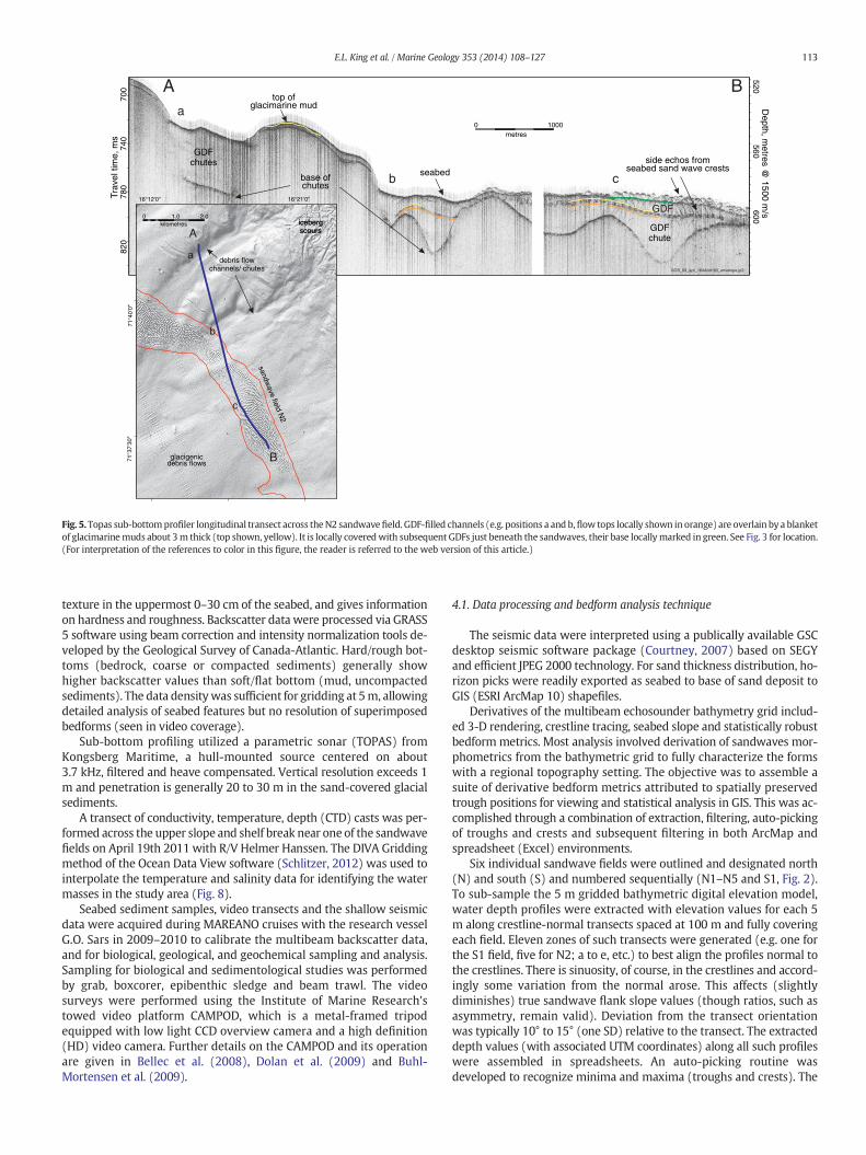
In the northern part of the study area, seaward of the mouth of theBear Island Trough, sub-bottom profiler data show that GDFs occur di-rectly below the seabed sand unit (Fig. 4). These are characterized bya stacked, braided pattern with relief of only meters or less (Fig. 2). In

the south they are blanketed with layered glacimarine deposits, locallyup to a fewmeters thick, in turn covered with thin sand and gravel lags.

There is a marked change from north to south in the presence ofdownslope channels or gullies with linear, dendritic and anastomosingpatterns, both buried and surficial (Figs. 2 and 3). Gullies in the southare typically 20–40 m deep, while they may be up to 150 m deeplower on the slope, where they merge. The gully cuts have lens shapedinfilling bodies with the acoustically semi-transparent, incoherent andhomogeneous signal characteristic of GDFs (Laberg and Vorren, 1995;Vorren et al., 1998; Laberg et al., 2010). They are interpreted to repre-sent cohesive mass transport, debris flow deposits similar to depositson the North Sea Fan (Nygård et al., 2002). We interpret the gullies tobe formed by debris flow activity (some initiated at sediment slidesites) emanating from the ice margin on Tromsøflaket and term themGDF chutes. The chutes are usually, but not exclusively, devoid of a cap-ping glacimarine blanket (Fig. 5, position a) in contrast to themore con-tinuous blanket over GDFs outside the gullies. It is unclear if thisrepresents GDF activity synchronous to the interfluve glacimarine blan-ket (and assimilation) or later (current) removal. The thalwegs are oc-casionally sandy at the immediate seabed, contrasting with ubiquitousgravel elsewhere.

Thus, cold and dense glacial margin-derived meltwater could havebeen instrumental in some of the chute history. Vorren et al. (1989)recognized these chutes (gullies) but attributed an interglacialcold (winter), dense shelf water and downslope transport process(cascading) on the basis that they are basically sediment-free (bypass

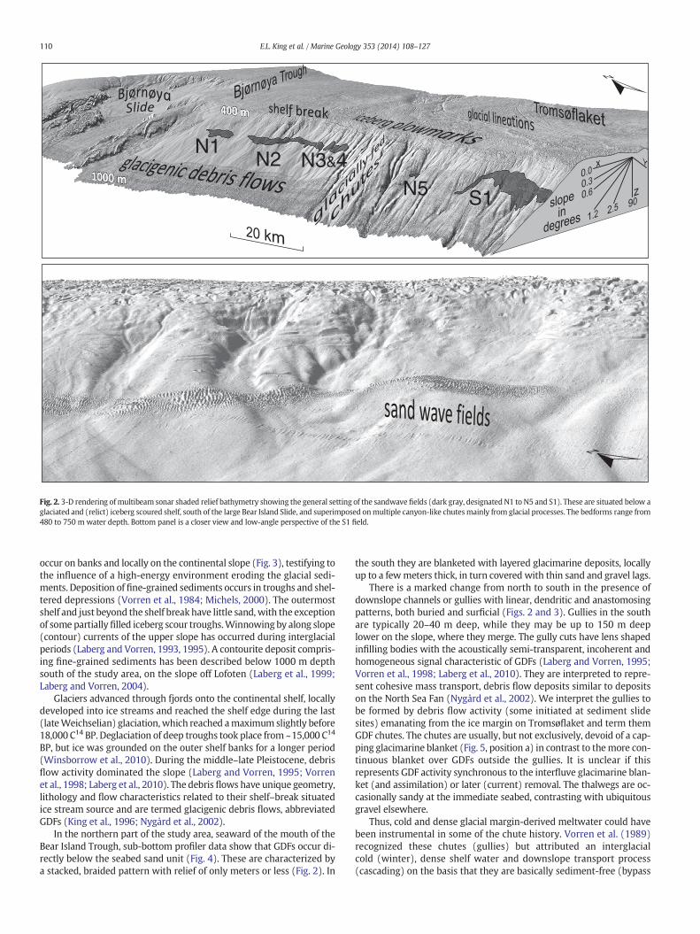
Fig. 3.Outline of the sandwave fields in the context of the MAREANO surficial geology (genesis) map (Bellec et al., 2012a and b). Also shown are sample, video, map and seismicillustration locations.


550600

sandwaves

Depth, m

etres @ 1500 m

/s

sandwave field boundary

base of GDFchute channel

GDF 1

GDF 2

F G

head ofchute

erosion?

stratifiedglacimarine mud

sandwaves

750

800

glacimarine mud

glacimarine mudwith sand cover

glacimarine mudwith sand cover

550600

Depth, m

etres @ 1500 m

/s

sandwavesC D

D0 500

metres

E

71°4

'0"

0 1 2

kilometres

C

D

E

17°0'0"

71°8

'0"

F

G780

830

730

Tra

vel t

ime,

ms

825775

725675

800

900

1000

Tra

vel t

ime,

ms

Depth, m

etres @ 1500 m

/s

GDF 2

GDF 2

GDF 1

Fig. 4. Topas sub-bottom profiler transect across the S1 sandwave field. The lower panel (C–D) connects with the larger (D–E). Small sandwaves lie on top of stratified glacimarinesediments. See Fig. 3 for location.


sites). This is also the interpreted transport mechanism for long-termfeeding of muddy contourites off the Spitsbergen margin (Rudelset al., 1999), but inferredduring glacials. The 1989work predated recog-nition of the GDF phenomenon and utilized low-resolution seismic, un-able to resolve them in the partially filled gullies. The Spitsbergen workrecognized intercalation of drift horizons and GDFs, much like observedhere (Fig. 5, positions b and c). Cold and dense glacial margin-derivedmeltwater could have been instrumental in occasional removal orpreventing deposition of the glacimarine blanket in the thalwegs. A lim-ited post-glacial sandy downslope transport is considered in a laterSection (6.3).

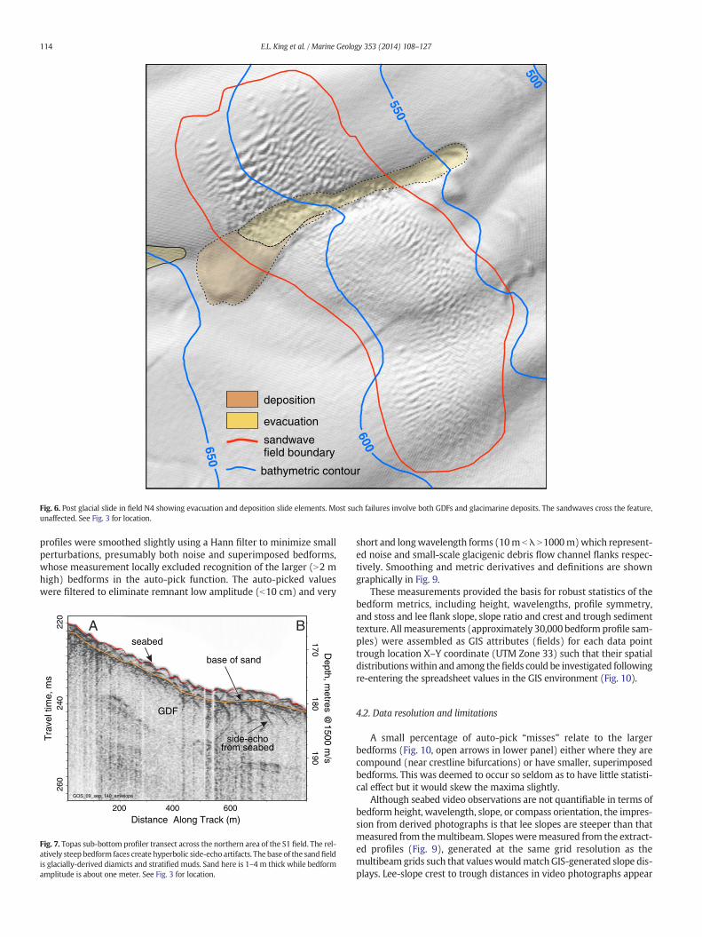
Several large, submarine slides of poorly constrained age have oc-curred in the central and southern parts of the study area but aremainlycovered by debris flow deposits and glacimarine sediments and presentlittle seabed expression. Smaller slides with good seabed expression arescattered over the study area. At least 23 slides were identified within10 km of the sandwave fields. These range from 0.5 to 4 km2 and cutglacimarine sediments, post-dating the GDFs (Fig. 6).

The sands comprising the sandwaves lie on top of the GDFs or theglacimarine blanket (Fig. 7). They are invariably thin, the majority ofsand within the sandwave itself, and it is common that the sandwavetroughs coincide with the gravel lag marking the top of the glacigenicsediments.

3. Oceanographic setting

The North Atlantic Current (NAC) (Norwegian Atlantic Current,NwAC along the Norwegian margin) carries warm and saline North At-lantic Water (NAW) into the Nordic Seas (Fig. 8). The NAC splits in twobranches west of Tromsøflaket. One branch follows the continental

slope north–northwestwards toward Svalbard, while one branchswings into the Barents Sea. The Norwegian Coastal Current also flowsnorth, along the coast (Rudels et al., 1999).

Three well defined water masses are differentiated offshoreLofoten–Vesterålen–Troms along the NW Norwegian continental slope(e.g. Helland-Hansen and Nansen, 1909; Hopkins, 1991; Hansen andØsterhus, 2000). North Atlantic Water (NAW) is characterized bysalinityN 35, and is typically found on the upper slope shallower thanca. 700 m depth. NAW has temperatures above 6 °C at the mid-Norwegian margin (Haugan et al., 1991) and flows northeastwardsalong the slope with typical current speeds of 0.2–0.4 m/s(Heathershaw et al., 1998) but occasionally reaching surface velocitiesin excess of 1 m/s west of Lofoten and Vesterålen (Poulain et al.,1996). Norwegian Sea Arctic Intermediate Water (NSAIW) occurs atca. 700–1000 m depth with temperatures between 0.5 °C and −0.5 °Cand is less saline than the water masses above and below (Hansenand Østerhus, 2000). Norwegian Sea Deep Water (NSDW) occursbelow ca. 1000 m with temperature below −0.5 °C (Hansen andØsterhus, 2000). The depth of the transition zone between the waterlayers varies throughout the year, deepening in the winter, and longwavelength internal waves may occur.

4. Methods

The study area (Fig. 1) was mapped by multibeam echosounder(Kongsberg Simrad EM710, 70–100 kHz range) by the NorwegianDefence Research Establishment/Norwegian Mapping Authority in2008–2009 as part of the MAREANO program. The multibeamechosounder provides two datasets: bathymetry and backscatter. Thebackscatter (acoustic reflectance) is influenced mainly by sediment

Trav

el ti

me,

ms

GOS_09_apr_164And165_envelope.jp2

Depth, m

etres @ 1500 m

/s

16°21'0"16°12'0"

71°4

0'0"

71°3

7'30

"

icebergscoursicebergscours

debris flowchannels/ chutes

GDFchute

GDFchutes

sandwave field N

2

A

top ofglacimarine mud

side echos fromseabed sand wave crests

700

740

780

820

600560

520

a

a

A B

base ofchutes

seabedb c

GDF

c

b

glacigenicdebris flows

B

0 2.01.0kilometres

0 1000metres

Fig. 5.Topas sub-bottomprofiler longitudinal transect across theN2 sandwavefield. GDF-filled channels (e.g. positions a and b,flow tops locally shown in orange) are overlain by a blanketof glacimarinemuds about 3m thick (top shown, yellow). It is locally coveredwith subsequent GDFs just beneath the sandwaves, their base locallymarked in green. See Fig. 3 for location.(For interpretation of the references to color in this figure, the reader is referred to the web version of this article.)


texture in the uppermost 0–30 cm of the seabed, and gives informationon hardness and roughness. Backscatter data were processed via GRASS5 software using beam correction and intensity normalization tools de-veloped by the Geological Survey of Canada-Atlantic. Hard/rough bot-toms (bedrock, coarse or compacted sediments) generally showhigher backscatter values than soft/flat bottom (mud, uncompactedsediments). The data densitywas sufficient for gridding at 5m, allowingdetailed analysis of seabed features but no resolution of superimposedbedforms (seen in video coverage).

Sub-bottom profiling utilized a parametric sonar (TOPAS) fromKongsberg Maritime, a hull-mounted source centered on about3.7 kHz, filtered and heave compensated. Vertical resolution exceeds 1m and penetration is generally 20 to 30 m in the sand-covered glacialsediments.

A transect of conductivity, temperature, depth (CTD) casts was per-formed across the upper slope and shelf break near one of the sandwavefields on April 19th 2011 with R/V Helmer Hanssen. The DIVA Griddingmethod of the Ocean Data View software (Schlitzer, 2012) was used tointerpolate the temperature and salinity data for identifying the watermasses in the study area (Fig. 8).

Seabed sediment samples, video transects and the shallow seismicdata were acquired during MAREANO cruises with the research vesselG.O. Sars in 2009–2010 to calibrate the multibeam backscatter data,and for biological, geological, and geochemical sampling and analysis.Sampling for biological and sedimentological studies was performedby grab, boxcorer, epibenthic sledge and beam trawl. The videosurveys were performed using the Institute of Marine Research'stowed video platform CAMPOD, which is a metal-framed tripodequipped with low light CCD overview camera and a high definition(HD) video camera. Further details on the CAMPOD and its operationare given in Bellec et al. (2008), Dolan et al. (2009) and Buhl-Mortensen et al. (2009).

4.1. Data processing and bedform analysis technique

The seismic data were interpreted using a publically available GSCdesktop seismic software package (Courtney, 2007) based on SEGYand efficient JPEG 2000 technology. For sand thickness distribution, ho-rizon picks were readily exported as seabed to base of sand deposit toGIS (ESRI ArcMap 10) shapefiles.

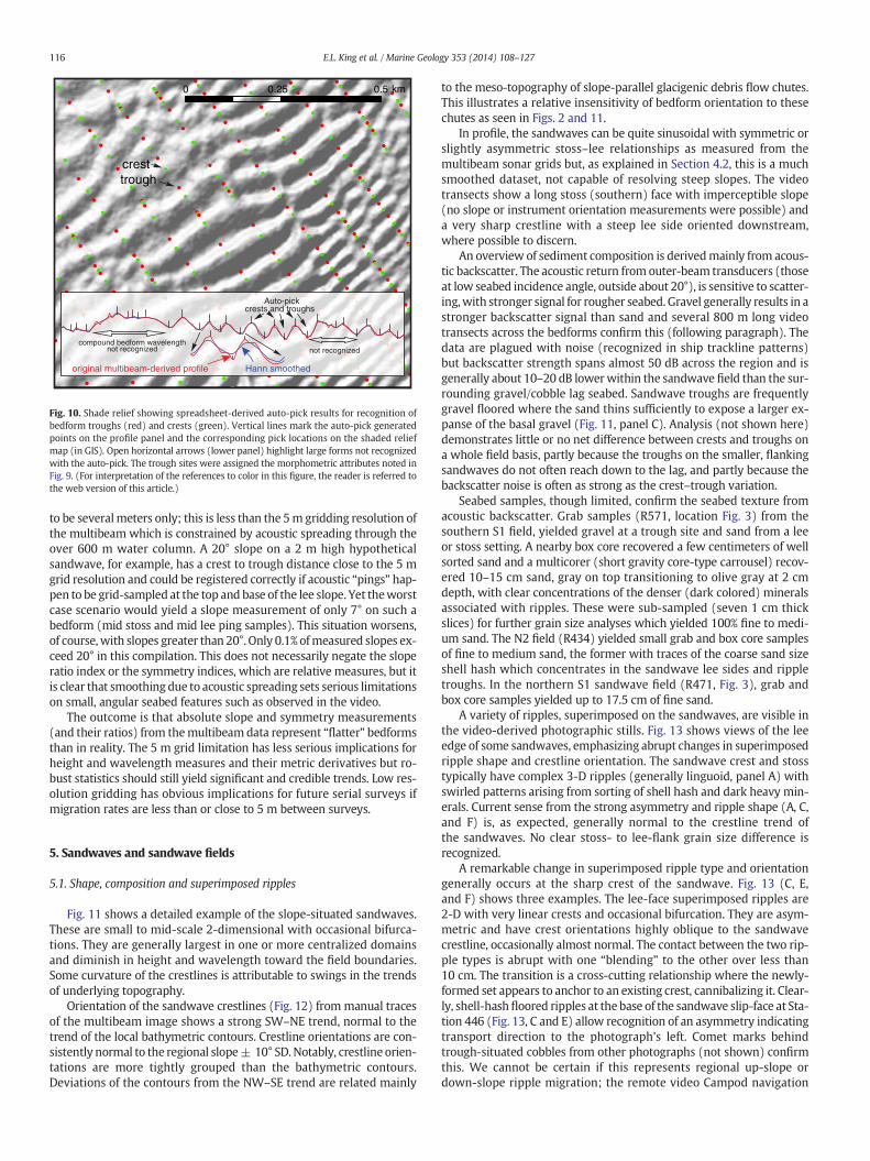
Derivatives of the multibeam echosounder bathymetry grid includ-ed 3-D rendering, crestline tracing, seabed slope and statistically robustbedform metrics. Most analysis involved derivation of sandwaves mor-phometrics from the bathymetric grid to fully characterize the formswith a regional topography setting. The objective was to assemble asuite of derivative bedform metrics attributed to spatially preservedtrough positions for viewing and statistical analysis in GIS. This was ac-complished through a combination of extraction, filtering, auto-pickingof troughs and crests and subsequent filtering in both ArcMap andspreadsheet (Excel) environments.

Six individual sandwave fields were outlined and designated north(N) and south (S) and numbered sequentially (N1–N5 and S1, Fig. 2).To sub-sample the 5 m gridded bathymetric digital elevation model,water depth profiles were extracted with elevation values for each 5m along crestline-normal transects spaced at 100 m and fully coveringeach field. Eleven zones of such transects were generated (e.g. one forthe S1 field, five for N2; a to e, etc.) to best align the profiles normal tothe crestlines. There is sinuosity, of course, in the crestlines and accord-ingly some variation from the normal arose. This affects (slightlydiminishes) true sandwave flank slope values (though ratios, such asasymmetry, remain valid). Deviation from the transect orientationwas typically 10° to 15° (one SD) relative to the transect. The extracteddepth values (with associated UTM coordinates) along all such profileswere assembled in spreadsheets. An auto-picking routine wasdeveloped to recognize minima and maxima (troughs and crests). The

600

550

650

deposition

evacuation

sandwavefield boundary

bathymetric contour

Fig. 6. Post glacial slide in field N4 showing evacuation and deposition slide elements. Most such failures involve both GDFs and glacimarine deposits. The sandwaves cross the feature,unaffected. See Fig. 3 for location.


profiles were smoothed slightly using a Hann filter to minimize smallperturbations, presumably both noise and superimposed bedforms,whose measurement locally excluded recognition of the larger (N2 mhigh) bedforms in the auto-pick function. The auto-picked valueswere filtered to eliminate remnant low amplitude (b10 cm) and very

seabed

base of sand

GDF

side-echofrom seabed

GOS_09_sep_140_envelope

Distance Along Track (m) 200 400 600

220

240

260

190180

170 Depth, m

etres @1500 m

/s

Tra

vel t

ime,

ms

A B

Fig. 7. Topas sub-bottom profiler transect across the northern area of the S1 field. The rel-atively steep bedform faces create hyperbolic side-echo artifacts. The base of the sandfieldis glacially-derived diamicts and stratified muds. Sand here is 1–4 m thick while bedformamplitude is about one meter. See Fig. 3 for location.

short and longwavelength forms (10m b λ N1000m)which represent-ed noise and small-scale glacigenic debris flow channel flanks respec-tively. Smoothing and metric derivatives and definitions are showngraphically in Fig. 9.

These measurements provided the basis for robust statistics of thebedform metrics, including height, wavelengths, profile symmetry,and stoss and lee flank slope, slope ratio and crest and trough sedimenttexture. All measurements (approximately 30,000 bedform profile sam-ples) were assembled as GIS attributes (fields) for each data pointtrough location X–Y coordinate (UTM Zone 33) such that their spatialdistributionswithin and among thefields could be investigated followingre-entering the spreadsheet values in the GIS environment (Fig. 10).

4.2. Data resolution and limitations

A small percentage of auto-pick “misses” relate to the largerbedforms (Fig. 10, open arrows in lower panel) either where they arecompound (near crestline bifurcations) or have smaller, superimposedbedforms. This was deemed to occur so seldom as to have little statisti-cal effect but it would skew the maxima slightly.

Although seabed video observations are not quantifiable in terms ofbedform height, wavelength, slope, or compass orientation, the impres-sion from derived photographs is that lee slopes are steeper than thatmeasured from themultibeam. Slopesweremeasured from the extract-ed profiles (Fig. 9), generated at the same grid resolution as themultibeam grids such that valueswouldmatchGIS-generated slope dis-plays. Lee-slope crest to trough distances in video photographs appear

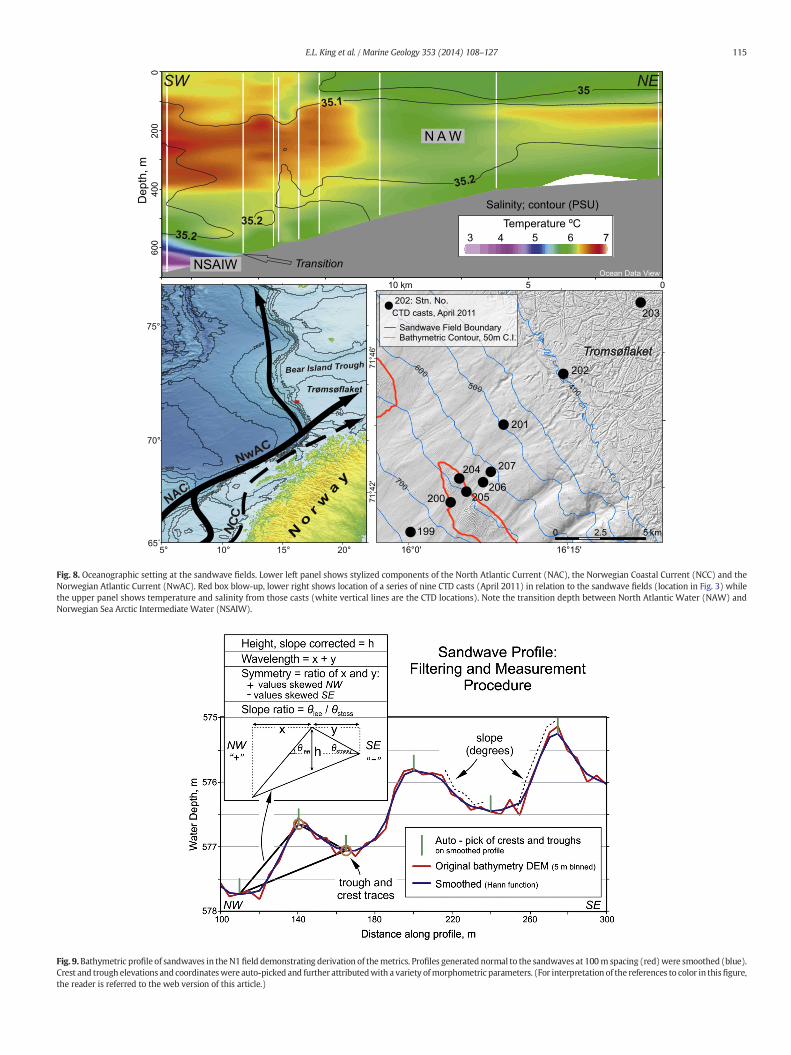
Fig. 9.Bathymetric profile of sandwaves in theN1field demonstrating derivation of themetrics. Profiles generated normal to the sandwaves at 100m spacing (red)were smoothed (blue).Crest and trough elevations and coordinateswere auto-picked and further attributedwith a variety ofmorphometric parameters. (For interpretation of the references to color in thisfigure,the reader is referred to the web version of this article.)

Fig. 8. Oceanographic setting at the sandwave fields. Lower left panel shows stylized components of the North Atlantic Current (NAC), the Norwegian Coastal Current (NCC) and theNorwegian Atlantic Current (NwAC). Red box blow-up, lower right shows location of a series of nine CTD casts (April 2011) in relation to the sandwave fields (location in Fig. 3) whilethe upper panel shows temperature and salinity from those casts (white vertical lines are the CTD locations). Note the transition depth between North Atlantic Water (NAW) andNorwegian Sea Arctic Intermediate Water (NSAIW).


cresttrough

Auto-pickcrests and troughs

Hann smoothed

compound bedform wavelengthnot recognized not recognized

original multibeam-derived profile

0 0.25 0.5 km

Fig. 10. Shade relief showing spreadsheet-derived auto-pick results for recognition ofbedform troughs (red) and crests (green). Vertical lines mark the auto-pick generatedpoints on the profile panel and the corresponding pick locations on the shaded reliefmap (in GIS). Open horizontal arrows (lower panel) highlight large forms not recognizedwith the auto-pick. The trough sites were assigned the morphometric attributes noted inFig. 9. (For interpretation of the references to color in this figure, the reader is referred tothe web version of this article.)


to be severalmeters only; this is less than the 5m gridding resolution ofthe multibeam which is constrained by acoustic spreading through theover 600 m water column. A 20° slope on a 2 m high hypotheticalsandwave, for example, has a crest to trough distance close to the 5 mgrid resolution and could be registered correctly if acoustic “pings” hap-pen to be grid-sampled at the top and base of the lee slope. Yet theworstcase scenario would yield a slope measurement of only 7° on such abedform (mid stoss and mid lee ping samples). This situation worsens,of course,with slopes greater than 20°. Only 0.1%ofmeasured slopes ex-ceed 20° in this compilation. This does not necessarily negate the sloperatio index or the symmetry indices, which are relative measures, but itis clear that smoothing due to acoustic spreading sets serious limitationson small, angular seabed features such as observed in the video.

The outcome is that absolute slope and symmetry measurements(and their ratios) from themultibeam data represent “flatter” bedformsthan in reality. The 5 m grid limitation has less serious implications forheight and wavelength measures and their metric derivatives but ro-bust statistics should still yield significant and credible trends. Low res-olution gridding has obvious implications for future serial surveys ifmigration rates are less than or close to 5 m between surveys.

5. Sandwaves and sandwave fields

5.1. Shape, composition and superimposed ripples

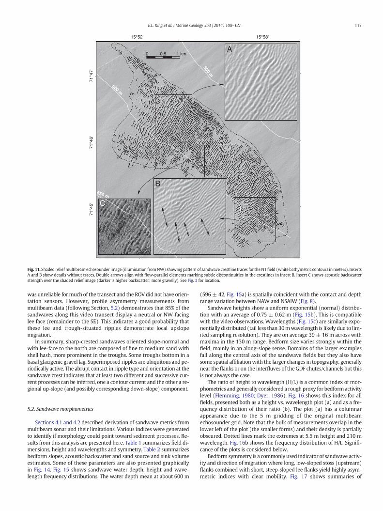
Fig. 11 shows a detailed example of the slope-situated sandwaves.These are small to mid-scale 2-dimensional with occasional bifurca-tions. They are generally largest in one or more centralized domainsand diminish in height and wavelength toward the field boundaries.Some curvature of the crestlines is attributable to swings in the trendsof underlying topography.

Orientation of the sandwave crestlines (Fig. 12) from manual tracesof the multibeam image shows a strong SW–NE trend, normal to thetrend of the local bathymetric contours. Crestline orientations are con-sistently normal to the regional slope± 10° SD. Notably, crestline orien-tations are more tightly grouped than the bathymetric contours.Deviations of the contours from the NW–SE trend are related mainly

to the meso-topography of slope-parallel glacigenic debris flow chutes.This illustrates a relative insensitivity of bedform orientation to thesechutes as seen in Figs. 2 and 11.

In profile, the sandwaves can be quite sinusoidal with symmetric orslightly asymmetric stoss–lee relationships as measured from themultibeam sonar grids but, as explained in Section 4.2, this is a muchsmoothed dataset, not capable of resolving steep slopes. The videotransects show a long stoss (southern) face with imperceptible slope(no slope or instrument orientation measurements were possible) anda very sharp crestline with a steep lee side oriented downstream,where possible to discern.

An overview of sediment composition is derivedmainly from acous-tic backscatter. The acoustic return from outer-beam transducers (thoseat low seabed incidence angle, outside about 20°), is sensitive to scatter-ing,with stronger signal for rougher seabed. Gravel generally results in astronger backscatter signal than sand and several 800 m long videotransects across the bedforms confirm this (following paragraph). Thedata are plagued with noise (recognized in ship trackline patterns)but backscatter strength spans almost 50 dB across the region and isgenerally about 10–20 dB lowerwithin the sandwave field than the sur-rounding gravel/cobble lag seabed. Sandwave troughs are frequentlygravel floored where the sand thins sufficiently to expose a larger ex-panse of the basal gravel (Fig. 11, panel C). Analysis (not shown here)demonstrates little or no net difference between crests and troughs ona whole field basis, partly because the troughs on the smaller, flankingsandwaves do not often reach down to the lag, and partly because thebackscatter noise is often as strong as the crest–trough variation.

Seabed samples, though limited, confirm the seabed texture fromacoustic backscatter. Grab samples (R571, location Fig. 3) from thesouthern S1 field, yielded gravel at a trough site and sand from a leeor stoss setting. A nearby box core recovered a few centimeters of wellsorted sand and a multicorer (short gravity core-type carrousel) recov-ered 10–15 cm sand, gray on top transitioning to olive gray at 2 cmdepth, with clear concentrations of the denser (dark colored) mineralsassociated with ripples. These were sub-sampled (seven 1 cm thickslices) for further grain size analyses which yielded 100% fine to medi-um sand. The N2 field (R434) yielded small grab and box core samplesof fine to medium sand, the former with traces of the coarse sand sizeshell hash which concentrates in the sandwave lee sides and rippletroughs. In the northern S1 sandwave field (R471, Fig. 3), grab andbox core samples yielded up to 17.5 cm of fine sand.

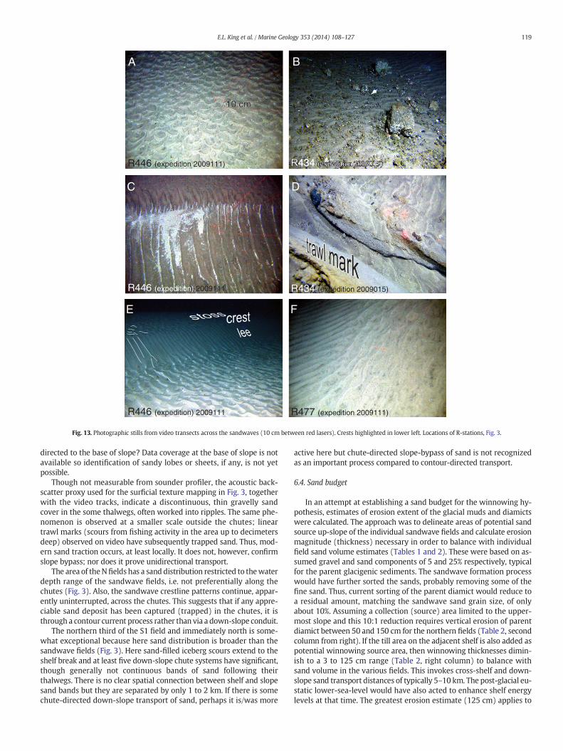
A variety of ripples, superimposed on the sandwaves, are visible inthe video-derived photographic stills. Fig. 13 shows views of the leeedge of some sandwaves, emphasizing abrupt changes in superimposedripple shape and crestline orientation. The sandwave crest and stosstypically have complex 3-D ripples (generally linguoid, panel A) withswirled patterns arising from sorting of shell hash and dark heavy min-erals. Current sense from the strong asymmetry and ripple shape (A, C,and F) is, as expected, generally normal to the crestline trend ofthe sandwaves. No clear stoss- to lee-flank grain size difference isrecognized.

A remarkable change in superimposed ripple type and orientationgenerally occurs at the sharp crest of the sandwave. Fig. 13 (C, E,and F) shows three examples. The lee-face superimposed ripples are2-D with very linear crests and occasional bifurcation. They are asym-metric and have crest orientations highly oblique to the sandwavecrestline, occasionally almost normal. The contact between the two rip-ple types is abrupt with one “blending” to the other over less than10 cm. The transition is a cross-cutting relationship where the newly-formed set appears to anchor to an existing crest, cannibalizing it. Clear-ly, shell-hashfloored ripples at the base of the sandwave slip-face at Sta-tion 446 (Fig. 13, C and E) allow recognition of an asymmetry indicatingtransport direction to the photograph's left. Comet marks behindtrough-situated cobbles from other photographs (not shown) confirmthis. We cannot be certain if this represents regional up-slope ordown-slope ripple migration; the remote video Campod navigation

15°58'15°52'

71°4

7'71

°46'

71°4

5'

0 1 km0.5

550 m

600 m

650 m

A

B

C

Fig. 11. Shaded reliefmultibeamechosounder image (illumination fromNW) showing pattern of sandwave crestline traces for theN1field (white bathymetric contours inmeters). InsertsA and B show details without traces. Double arrows align with flow-parallel elements marking subtle discontinuities in the crestlines in insert B. Insert C shows acoustic backscatterstrength over the shaded relief image (darker is higher backscatter; more gravelly). See Fig. 3 for location.


was unreliable for much of the transect and the ROV did not have orien-tation sensors. However, profile asymmetry measurements frommultibeam data (following Section, 5.2) demonstrates that 85% of thesandwaves along this video transect display a neutral or NW-facinglee face (remainder to the SE). This indicates a good probability thatthese lee and trough-situated ripples demonstrate local upslopemigration.

In summary, sharp-crested sandwaves oriented slope-normal andwith lee-face to the north are composed of fine to medium sand withshell hash, more prominent in the troughs. Some troughs bottom in abasal glacigenic gravel lag. Superimposed ripples are ubiquitous and pe-riodically active. The abrupt contact in ripple type and orientation at thesandwave crest indicates that at least two different and successive cur-rent processes can be inferred, one a contour current and the other a re-gional up-slope (and possibly corresponding down-slope) component.

5.2. Sandwave morphometrics

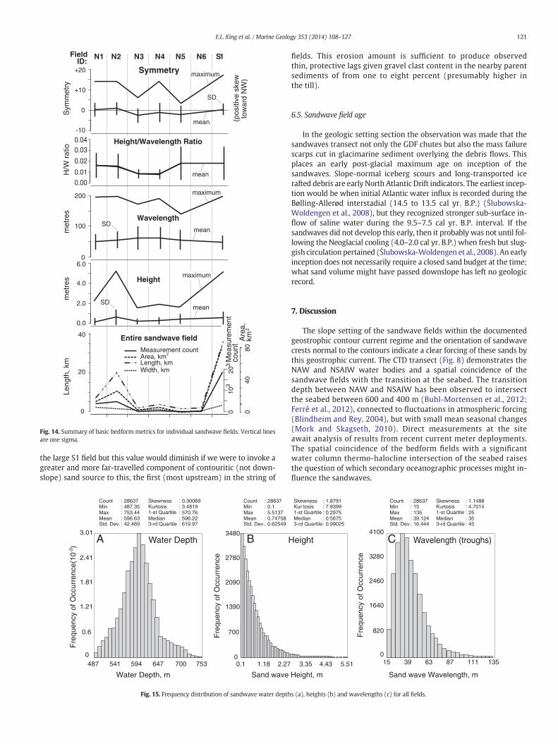
Sections 4.1 and 4.2 described derivation of sandwave metrics frommultibeam sonar and their limitations. Various indices were generatedto identify if morphology could point toward sediment processes. Re-sults from this analysis are presented here. Table 1 summarizes field di-mensions, height and wavelengths and symmetry. Table 2 summarizesbedform slopes, acoustic backscatter and sand source and sink volumeestimates. Some of these parameters are also presented graphicallyin Fig. 14. Fig. 15 shows sandwave water depth, height and wave-length frequency distributions. The water depth mean at about 600 m

(596 ± 42, Fig. 15a) is spatially coincident with the contact and depthrange variation between NAW and NSAIW (Fig. 8).

Sandwave heights show a uniform exponential (normal) distribu-tion with an average of 0.75 ± 0.62 m (Fig. 15b). This is compatiblewith the video observations. Wavelengths (Fig. 15c) are similarly expo-nentially distributed (tail less than 30mwavelength is likely due to lim-ited sampling resolution). They are on average 39 ± 16 m across withmaxima in the 130 m range. Bedform size varies strongly within thefield, mainly in an along-slope sense. Domains of the larger examplesfall along the central axis of the sandwave fields but they also havesome spatial affiliationwith the larger changes in topography, generallynear the flanks or on the interfluves of the GDF chutes/channels but thisis not always the case.

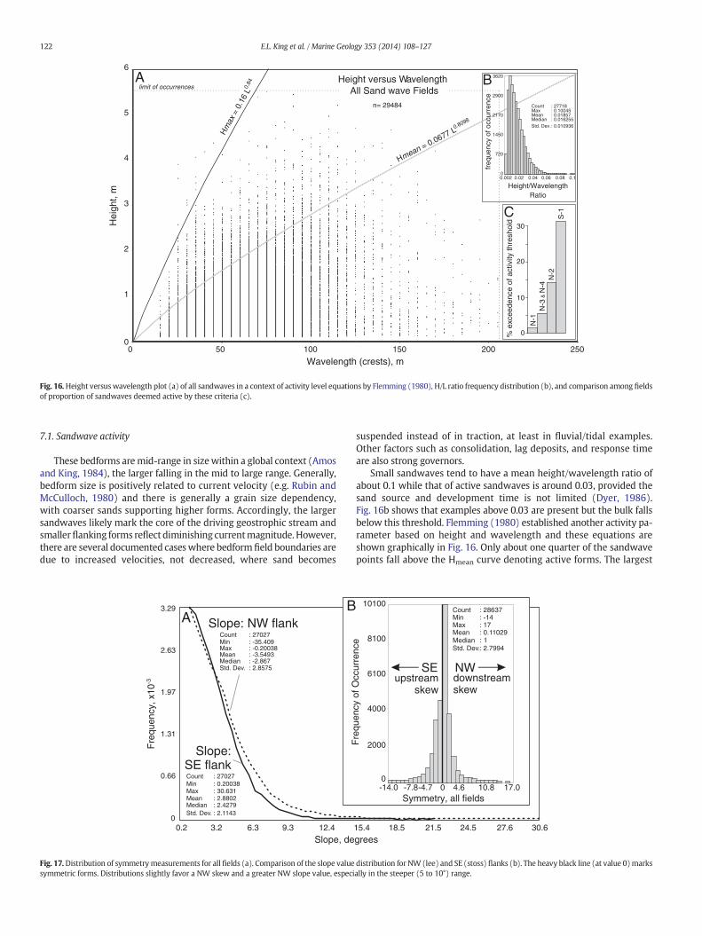
The ratio of height to wavelength (H/L) is a common index of mor-phometrics and generally considered a rough proxy for bedform activitylevel (Flemming, 1980; Dyer, 1986). Fig. 16 shows this index for allfields, presented both as a height vs. wavelength plot (a) and as a fre-quency distribution of their ratio (b). The plot (a) has a columnarappearance due to the 5 m gridding of the original multibeamechosounder grid. Note that the bulk of measurements overlap in thelower left of the plot (the smaller forms) and their density is partiallyobscured. Dotted lines mark the extremes at 5.5 m height and 210 mwavelength. Fig. 16b shows the frequency distribution of H/L. Signifi-cance of the plots is considered below.

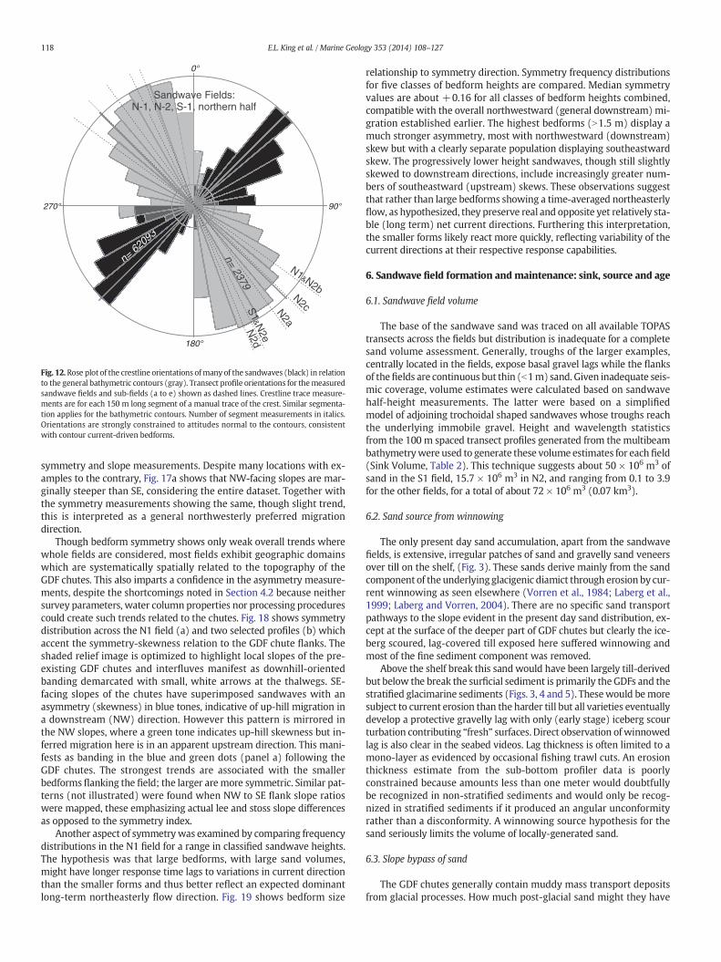
Bedform symmetry is a commonly used indicator of sandwave activ-ity and direction of migration where long, low-sloped stoss (upstream)flanks combined with short, steep-sloped lee flanks yield highly asym-metric indices with clear mobility. Fig. 17 shows summaries of

0°

90°

180°

270°

n= 62

093

Sandwave Fields:N-1, N-2, S-1, northern half

N1&N2b

N2a

N2c

N2d

n= 2379S

1&N

2e

Fig. 12. Rose plot of the crestline orientations ofmany of the sandwaves (black) in relationto the general bathymetric contours (gray). Transect profile orientations for themeasuredsandwave fields and sub-fields (a to e) shown as dashed lines. Crestline trace measure-ments are for each 150 m long segment of a manual trace of the crest. Similar segmenta-tion applies for the bathymetric contours. Number of segment measurements in italics.Orientations are strongly constrained to attitudes normal to the contours, consistentwith contour current-driven bedforms.


symmetry and slope measurements. Despite many locations with ex-amples to the contrary, Fig. 17a shows that NW-facing slopes are mar-ginally steeper than SE, considering the entire dataset. Together withthe symmetry measurements showing the same, though slight trend,this is interpreted as a general northwesterly preferred migrationdirection.

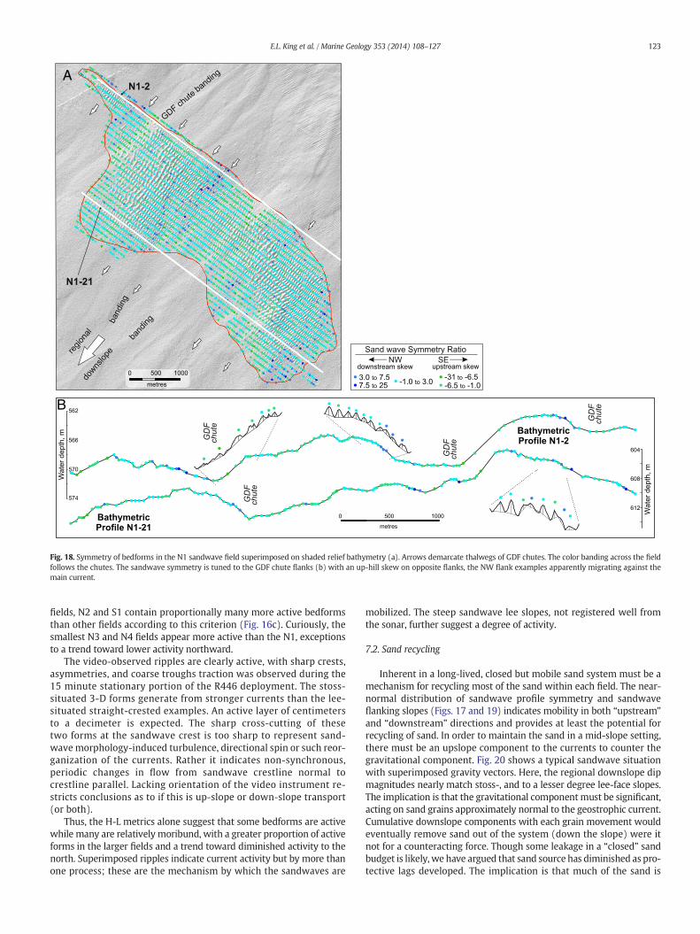
Though bedform symmetry shows only weak overall trends wherewhole fields are considered, most fields exhibit geographic domainswhich are systematically spatially related to the topography of theGDF chutes. This also imparts a confidence in the asymmetry measure-ments, despite the shortcomings noted in Section 4.2 because neithersurvey parameters, water column properties nor processing procedurescould create such trends related to the chutes. Fig. 18 shows symmetrydistribution across the N1 field (a) and two selected profiles (b) whichaccent the symmetry-skewness relation to the GDF chute flanks. Theshaded relief image is optimized to highlight local slopes of the pre-existing GDF chutes and interfluves manifest as downhill-orientedbanding demarcated with small, white arrows at the thalwegs. SE-facing slopes of the chutes have superimposed sandwaves with anasymmetry (skewness) in blue tones, indicative of up-hill migration ina downstream (NW) direction. However this pattern is mirrored inthe NW slopes, where a green tone indicates up-hill skewness but in-ferred migration here is in an apparent upstream direction. This mani-fests as banding in the blue and green dots (panel a) following theGDF chutes. The strongest trends are associated with the smallerbedforms flanking the field; the larger aremore symmetric. Similar pat-terns (not illustrated) were found when NW to SE flank slope ratioswere mapped, these emphasizing actual lee and stoss slope differencesas opposed to the symmetry index.

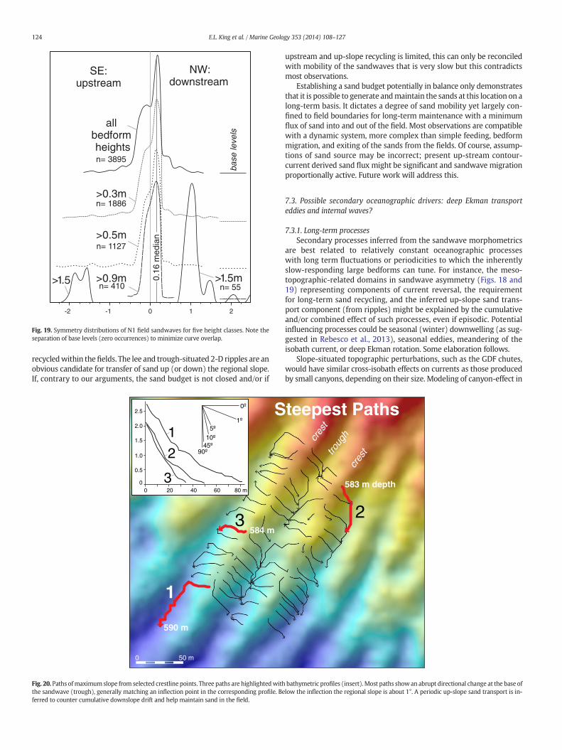
Another aspect of symmetrywas examined by comparing frequencydistributions in the N1 field for a range in classified sandwave heights.The hypothesis was that large bedforms, with large sand volumes,might have longer response time lags to variations in current directionthan the smaller forms and thus better reflect an expected dominantlong-term northeasterly flow direction. Fig. 19 shows bedform size

relationship to symmetry direction. Symmetry frequency distributionsfor five classes of bedform heights are compared. Median symmetryvalues are about +0.16 for all classes of bedform heights combined,compatible with the overall northwestward (general downstream) mi-gration established earlier. The highest bedforms (N1.5 m) display amuch stronger asymmetry, most with northwestward (downstream)skew but with a clearly separate population displaying southeastwardskew. The progressively lower height sandwaves, though still slightlyskewed to downstream directions, include increasingly greater num-bers of southeastward (upstream) skews. These observations suggestthat rather than large bedforms showing a time-averaged northeasterlyflow, as hypothesized, they preserve real and opposite yet relatively sta-ble (long term) net current directions. Furthering this interpretation,the smaller forms likely react more quickly, reflecting variability of thecurrent directions at their respective response capabilities.

6. Sandwave field formation andmaintenance: sink, source and age

6.1. Sandwave field volume

The base of the sandwave sand was traced on all available TOPAStransects across the fields but distribution is inadequate for a completesand volume assessment. Generally, troughs of the larger examples,centrally located in the fields, expose basal gravel lags while the flanksof thefields are continuous but thin (b1m) sand. Given inadequate seis-mic coverage, volume estimates were calculated based on sandwavehalf-height measurements. The latter were based on a simplifiedmodel of adjoining trochoidal shaped sandwaves whose troughs reachthe underlying immobile gravel. Height and wavelength statisticsfrom the 100 m spaced transect profiles generated from the multibeambathymetrywere used to generate these volume estimates for eachfield(Sink Volume, Table 2). This technique suggests about 50 × 106 m3 ofsand in the S1 field, 15.7 × 106 m3 in N2, and ranging from 0.1 to 3.9for the other fields, for a total of about 72 × 106 m3 (0.07 km3).

6.2. Sand source from winnowing

The only present day sand accumulation, apart from the sandwavefields, is extensive, irregular patches of sand and gravelly sand veneersover till on the shelf, (Fig. 3). These sands derive mainly from the sandcomponent of the underlying glacigenic diamict through erosion by cur-rent winnowing as seen elsewhere (Vorren et al., 1984; Laberg et al.,1999; Laberg and Vorren, 2004). There are no specific sand transportpathways to the slope evident in the present day sand distribution, ex-cept at the surface of the deeper part of GDF chutes but clearly the ice-berg scoured, lag-covered till exposed here suffered winnowing andmost of the fine sediment component was removed.

Above the shelf break this sandwould have been largely till-derivedbut below the break the surficial sediment is primarily the GDFs and thestratified glacimarine sediments (Figs. 3, 4 and 5). Thesewould bemoresubject to current erosion than the harder till but all varieties eventuallydevelop a protective gravelly lag with only (early stage) iceberg scourturbation contributing “fresh” surfaces. Direct observation ofwinnowedlag is also clear in the seabed videos. Lag thickness is often limited to amono-layer as evidenced by occasional fishing trawl cuts. An erosionthickness estimate from the sub-bottom profiler data is poorlyconstrained because amounts less than one meter would doubtfullybe recognized in non-stratified sediments and would only be recog-nized in stratified sediments if it produced an angular unconformityrather than a disconformity. A winnowing source hypothesis for thesand seriously limits the volume of locally-generated sand.

6.3. Slope bypass of sand

The GDF chutes generally contain muddy mass transport depositsfrom glacial processes. How much post-glacial sand might they have

R477 (expedition 2009111)


R446 (expedition) 2009111

R446 (expedition) 2009111

RR434


10 cm10 cm

A

C

E

B

D

F

Fig. 13. Photographic stills from video transects across the sandwaves (10 cm between red lasers). Crests highlighted in lower left. Locations of R-stations, Fig. 3.


directed to the base of slope? Data coverage at the base of slope is notavailable so identification of sandy lobes or sheets, if any, is not yetpossible.

Though not measurable from sounder profiler, the acoustic back-scatter proxy used for the surficial texture mapping in Fig. 3, togetherwith the video tracks, indicate a discontinuous, thin gravelly sandcover in the some thalwegs, often worked into ripples. The same phe-nomenon is observed at a smaller scale outside the chutes; lineartrawl marks (scours from fishing activity in the area up to decimetersdeep) observed on video have subsequently trapped sand. Thus, mod-ern sand traction occurs, at least locally. It does not, however, confirmslope bypass; nor does it prove unidirectional transport.

The area of theNfields has a sand distribution restricted to thewaterdepth range of the sandwave fields, i.e. not preferentially along thechutes (Fig. 3). Also, the sandwave crestline patterns continue, appar-ently uninterrupted, across the chutes. This suggests that if any appre-ciable sand deposit has been captured (trapped) in the chutes, it isthrough a contour current process rather than via a down-slope conduit.

The northern third of the S1 field and immediately north is some-what exceptional because here sand distribution is broader than thesandwave fields (Fig. 3). Here sand-filled iceberg scours extend to theshelf break and at least five down-slope chute systems have significant,though generally not continuous bands of sand following theirthalwegs. There is no clear spatial connection between shelf and slopesand bands but they are separated by only 1 to 2 km. If there is somechute-directed down-slope transport of sand, perhaps it is/was more

active here but chute-directed slope-bypass of sand is not recognizedas an important process compared to contour-directed transport.

6.4. Sand budget

In an attempt at establishing a sand budget for the winnowing hy-pothesis, estimates of erosion extent of the glacial muds and diamictswere calculated. The approach was to delineate areas of potential sandsource up-slope of the individual sandwave fields and calculate erosionmagnitude (thickness) necessary in order to balance with individualfield sand volume estimates (Tables 1 and 2). These were based on as-sumed gravel and sand components of 5 and 25% respectively, typicalfor the parent glacigenic sediments. The sandwave formation processwould have further sorted the sands, probably removing some of thefine sand. Thus, current sorting of the parent diamict would reduce toa residual amount, matching the sandwave sand grain size, of onlyabout 10%. Assuming a collection (source) area limited to the upper-most slope and this 10:1 reduction requires vertical erosion of parentdiamict between 50 and 150 cm for the northern fields (Table 2, secondcolumn from right). If the till area on the adjacent shelf is also added aspotential winnowing source area, then winnowing thicknesses dimin-ish to a 3 to 125 cm range (Table 2, right column) to balance withsand volume in the various fields. This invokes cross-shelf and down-slope sand transport distances of typically 5–10 km. The post-glacial eu-static lower-sea-level would have also acted to enhance shelf energylevels at that time. The greatest erosion estimate (125 cm) applies to

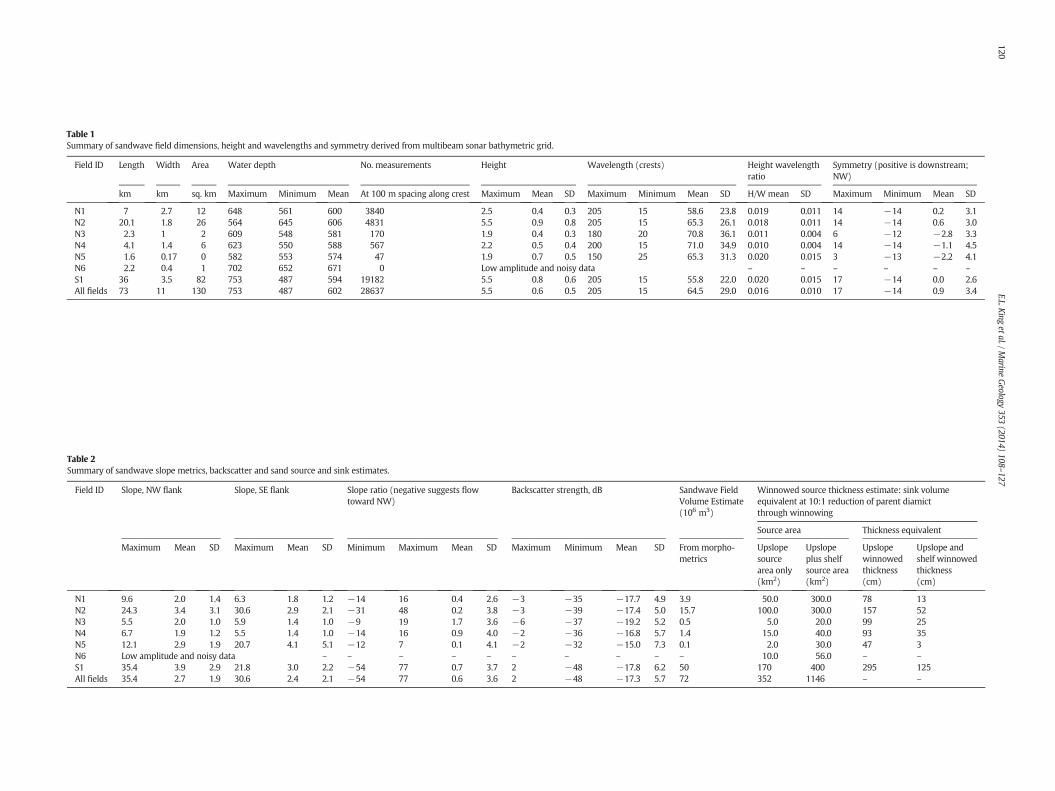
Table 1Summary of sandwave field dimensions, height and wavelengths and symmetry derived from multibeam sonar bathymetric grid.

Field ID Length Width Area Water depth No. measurements Height Wavelength (crests) Height wavelengthratio

Symmetry (positive is downstream;NW)

km km sq. km Maximum Minimum Mean At 100 m spacing along crest Maximum Mean SD Maximum Minimum Mean SD H/W mean SD Maximum Minimum Mean SD

N1 7 2.7 12 648 561 600 3840 2.5 0.4 0.3 205 15 58.6 23.8 0.019 0.011 14 −14 0.2 3.1N2 20.1 1.8 26 564 645 606 4831 5.5 0.9 0.8 205 15 65.3 26.1 0.018 0.011 14 −14 0.6 3.0N3 2.3 1 2 609 548 581 170 1.9 0.4 0.3 180 20 70.8 36.1 0.011 0.004 6 −12 −2.8 3.3N4 4.1 1.4 6 623 550 588 567 2.2 0.5 0.4 200 15 71.0 34.9 0.010 0.004 14 −14 −1.1 4.5N5 1.6 0.17 0 582 553 574 47 1.9 0.7 0.5 150 25 65.3 31.3 0.020 0.015 3 −13 −2.2 4.1N6 2.2 0.4 1 702 652 671 0 Low amplitude and noisy data – – – – – –

S1 36 3.5 82 753 487 594 19182 5.5 0.8 0.6 205 15 55.8 22.0 0.020 0.015 17 −14 0.0 2.6All fields 73 11 130 753 487 602 28637 5.5 0.6 0.5 205 15 64.5 29.0 0.016 0.010 17 −14 0.9 3.4

Table 2Summary of sandwave slope metrics, backscatter and sand source and sink estimates.

Field ID Slope, NW flank Slope, SE flank Slope ratio (negative suggests flowtoward NW)

Backscatter strength, dB Sandwave FieldVolume Estimate(106 m3)

Winnowed source thickness estimate: sink volumeequivalent at 10:1 reduction of parent diamictthrough winnowing

Source area Thickness equivalent

Maximum Mean SD Maximum Mean SD Minimum Maximum Mean SD Maximum Minimum Mean SD From morpho-metrics

Upslopesourcearea only(km2)

Upslopeplus shelfsource area(km2)

Upslopewinnowedthickness(cm)

Upslope andshelf winnowedthickness(cm)

N1 9.6 2.0 1.4 6.3 1.8 1.2 −14 16 0.4 2.6 −3 −35 −17.7 4.9 3.9 50.0 300.0 78 13N2 24.3 3.4 3.1 30.6 2.9 2.1 −31 48 0.2 3.8 −3 −39 −17.4 5.0 15.7 100.0 300.0 157 52N3 5.5 2.0 1.0 5.9 1.4 1.0 −9 19 1.7 3.6 −6 −37 −19.2 5.2 0.5 5.0 20.0 99 25N4 6.7 1.9 1.2 5.5 1.4 1.0 −14 16 0.9 4.0 −2 −36 −16.8 5.7 1.4 15.0 40.0 93 35N5 12.1 2.9 1.9 20.7 4.1 5.1 −12 7 0.1 4.1 −2 −32 −15.0 7.3 0.1 2.0 30.0 47 3N6 Low amplitude and noisy data – – – – – – – – – – 10.0 56.0 – –

S1 35.4 3.9 2.9 21.8 3.0 2.2 −54 77 0.7 3.7 2 −48 −17.8 6.2 50 170 400 295 125All fields 35.4 2.7 1.9 30.6 2.4 2.1 −54 77 0.6 3.6 2 −48 −17.3 5.7 72 352 1146 – –

120E.L.K

ingetal./M

arineGeology

353(2014)

108–127

0

Leng

th, k

mm

etre

sm

etre

s S

ymm

etry

H/W

rat

io

Mea

sure

men

tco

unt

20

40

Field ID:

N1 N2 N3 N4 N5 N6 S1

mean

mean

mean

mean

020

310

3

0.0

2.0

4.0

6.00

100

200

-10

0

+10

+20

0.000.01

0.02

0.030.04

(pos

itive

ske

wto

war

d N

W)

040

802

Are

a,km

Symmetry

Height/Wavelength Ratio

Wavelength

Height

Entire sandwave field

maximum

maximum

maximum

SD

SD

SD

Length, kmWidth, km

2Area, kmMeasurement count

Fig. 14. Summary of basic bedform metrics for individual sandwave fields. Vertical linesare one sigma.


the large S1 field but this value would diminish if we were to invoke agreater and more far-travelled component of contouritic (not down-slope) sand source to this, the first (most upstream) in the string of

487 541 594 647 700 7530

0.6

1.21

1.81

2.41

3.01

CountMinMaxMeanStd. Dev.

: 28637 : 487.35 : 753.44 : 596.63 : 42.469

SkewnessKurtosis1-st QuartileMedian3-rd Quartile

: 0.30069 : 3.4819 : 570.76 : 596.22 : 619.97

Fre

quen

cy o

f Occ

urre

nce(

10-3)

Water Depth, m

0.1 1.18 2.27

700

0

1390

2090

2780

3480


: 28637 : 0.1 : 5.5137 : 0.74758 : 0.62549

HWater Depth

Fre

quen

cy o

f Occ

urre

nce

Sand wave

BA

Fig. 15. Frequency distribution of sandwave water depth

fields. This erosion amount is sufficient to produce observedthin, protective lags given gravel clast content in the nearby parentsediments of from one to eight percent (presumably higher inthe till).

6.5. Sandwave field age

In the geologic setting section the observation was made that thesandwaves transect not only the GDF chutes but also the mass failurescarps cut in glacimarine sediment overlying the debris flows. Thisplaces an early post-glacial maximum age on inception of thesandwaves. Slope-normal iceberg scours and long-transported icerafted debris are early North Atlantic Drift indicators. The earliest incep-tion would be when initial Atlantic water influx is recorded during theBølling-Allerød interstadial (14.5 to 13.5 cal yr. B.P.) (Ślubowska-Woldengen et al., 2008), but they recognized stronger sub-surface in-flow of saline water during the 9.5–7.5 cal yr. B.P. interval. If thesandwaves did not develop this early, then it probably was not until fol-lowing the Neoglacial cooling (4.0–2.0 cal yr. B.P.) when fresh but slug-gish circulation pertained (Ślubowska-Woldengen et al., 2008). An earlyinception does not necessarily require a closed sand budget at the time;what sand volume might have passed downslope has left no geologicrecord.

7. Discussion

The slope setting of the sandwave fields within the documentedgeostrophic contour current regime and the orientation of sandwavecrests normal to the contours indicate a clear forcing of these sands bythis geostrophic current. The CTD transect (Fig. 8) demonstrates theNAW and NSAIW water bodies and a spatial coincidence of thesandwave fields with the transition at the seabed. The transitiondepth between NAW and NSAIW has been observed to intersectthe seabed between 600 and 400 m (Buhl-Mortensen et al., 2012;Ferré et al., 2012), connected to fluctuations in atmospheric forcing(Blindheim and Rey, 2004), but with small mean seasonal changes(Mork and Skagseth, 2010). Direct measurements at the siteawait analysis of results from recent current meter deployments.The spatial coincidence of the bedform fields with a significantwater column thermo-halocline intersection of the seabed raisesthe question of which secondary oceanographic processes might in-fluence the sandwaves.

3.35 4.43 5.51

SkewnessKur tosis1-st QuartileMedian3-rd Quartile

: 1.8791 : 7.9399 : 0.2975 : 0.5675 : 0.99025

eight

Fre

quen

cy o

f Occ

urre

nce

Height, m Sand wave Wavelength, m

15 39 63 87 111 1350

820

1640

2460

3280

4100


: 28637 : 15 : 135 : 39.124 : 16.444

SkewnessKurtosis1-st QuartileMedian3-rd Quartile

: 1.1488 : 4.7014 : 25 : 35 : 45

Wavelength (troughs)C

s (a), heights (b) and wavelengths (c) for all fields.

50 100 150 200 250

Wavelength (crests), m

limit of occurrences

0.8098

Hmean = 0.0677 L

0

1

2

3

4

5

6

0

Hei

ght,

m

0.84

Hm

ax =

0.1

6 L

Height versus WavelengthAll Sand wave Fields

n= 29484

0.002 0.02 0.04 0.06 0.08 0.10

720

1450

2900

3620

CountMaxMean

Std. Dev.

: 27718 : 0.10045 : 0.01857

: 0.010936Median : 0.016255

Height/WavelengthRatio

freq

uenc

y of

occ

urre

nce

2170

N-3

& N

-4N

-2

N-1

S-1

% e

xcee

denc

e of

act

ivity

thre

shol

d

0

10

20

30

A B

C

Fig. 16.Height versuswavelength plot (a) of all sandwaves in a context of activity level equations by Flemming (1980), H/L ratio frequency distribution (b), and comparison among fieldsof proportion of sandwaves deemed active by these criteria (c).


7.1. Sandwave activity

These bedforms aremid-range in sizewithin a global context (Amosand King, 1984), the larger falling in the mid to large range. Generally,bedform size is positively related to current velocity (e.g. Rubin andMcCulloch, 1980) and there is generally a grain size dependency,with coarser sands supporting higher forms. Accordingly, the largersandwaves likely mark the core of the driving geostrophic stream andsmallerflanking forms reflect diminishing currentmagnitude. However,there are several documented caseswhere bedformfield boundaries aredue to increased velocities, not decreased, where sand becomes

Slope, de

Fre

quen

cy, x

10-3

0.2 3.2 6.3 9.3 12.40

0.66

1.31

1.97

2.63

3.29

Slope:SE flankCountMinMaxMean

Std. Dev.

: 27027 : 0.20038 : 30.631 : 2.8802

: 2.1143Median : 2.4279

CountMinMaxMean

Std. Dev.

: 27027 : -35.409 : -0.20038 : -3.5493

: 2.8575Median : -2.867

Slope: NW flankB

A

Fig. 17.Distribution of symmetrymeasurements for all fields (a). Comparison of the slope valuesymmetric forms. Distributions slightly favor a NW skew and a greater NW slope value, especi

suspended instead of in traction, at least in fluvial/tidal examples.Other factors such as consolidation, lag deposits, and response timeare also strong governors.

Small sandwaves tend to have a mean height/wavelength ratio ofabout 0.1 while that of active sandwaves is around 0.03, provided thesand source and development time is not limited (Dyer, 1986).Fig. 16b shows that examples above 0.03 are present but the bulk fallsbelow this threshold. Flemming (1980) established another activity pa-rameter based on height and wavelength and these equations areshown graphically in Fig. 16. Only about one quarter of the sandwavepoints fall above the Hmean curve denoting active forms. The largest

grees15.4 18.5 21.5 24.5 27.6 30.6

Fre

quen

cy o

f Occ

urre

nce

-14.0 -7.8-4.7 0 4.6 10.8 17.00

2000

4000

6100

8100

10100

Symmetry, all fields

upstreamskew

SEdownstreamskew

NW

CountMinMaxMean

Std. Dev.

: 28637 : -14 : 17 : 0.11029

: 2.7994Median : 1

distribution for NW (lee) and SE (stoss) flanks (b). The heavy black line (at value 0)marksally in the steeper (5 to 10°) range.

A

B

Fig. 18. Symmetry of bedforms in the N1 sandwave field superimposed on shaded relief bathymetry (a). Arrows demarcate thalwegs of GDF chutes. The color banding across the fieldfollows the chutes. The sandwave symmetry is tuned to the GDF chute flanks (b) with an up-hill skew on opposite flanks, the NW flank examples apparently migrating against themain current.


fields, N2 and S1 contain proportionally many more active bedformsthan other fields according to this criterion (Fig. 16c). Curiously, thesmallest N3 and N4 fields appear more active than the N1, exceptionsto a trend toward lower activity northward.

The video-observed ripples are clearly active, with sharp crests,asymmetries, and coarse troughs traction was observed during the15 minute stationary portion of the R446 deployment. The stoss-situated 3-D forms generate from stronger currents than the lee-situated straight-crested examples. An active layer of centimetersto a decimeter is expected. The sharp cross-cutting of thesetwo forms at the sandwave crest is too sharp to represent sand-wave morphology-induced turbulence, directional spin or such reor-ganization of the currents. Rather it indicates non-synchronous,periodic changes in flow from sandwave crestline normal tocrestline parallel. Lacking orientation of the video instrument re-stricts conclusions as to if this is up-slope or down-slope transport(or both).

Thus, the H-L metrics alone suggest that some bedforms are activewhile many are relatively moribund, with a greater proportion of activeforms in the larger fields and a trend toward diminished activity to thenorth. Superimposed ripples indicate current activity but by more thanone process; these are the mechanism by which the sandwaves are

mobilized. The steep sandwave lee slopes, not registered well fromthe sonar, further suggest a degree of activity.

7.2. Sand recycling

Inherent in a long-lived, closed but mobile sand system must be amechanism for recycling most of the sand within each field. The near-normal distribution of sandwave profile symmetry and sandwaveflanking slopes (Figs. 17 and 19) indicates mobility in both “upstream”

and “downstream” directions and provides at least the potential forrecycling of sand. In order to maintain the sand in a mid-slope setting,there must be an upslope component to the currents to counter thegravitational component. Fig. 20 shows a typical sandwave situationwith superimposed gravity vectors. Here, the regional downslope dipmagnitudes nearly match stoss-, and to a lesser degree lee-face slopes.The implication is that the gravitational componentmust be significant,acting on sand grains approximately normal to the geostrophic current.Cumulative downslope components with each grain movement wouldeventually remove sand out of the system (down the slope) were itnot for a counteracting force. Though some leakage in a “closed” sandbudget is likely, we have argued that sand source has diminished as pro-tective lags developed. The implication is that much of the sand is

SE:upstream

NW:downstream

-1-2 0 1 2

>0.3mn= 1886

allbedform heightsn= 3895

>0.5mn= 1127

>0.9mn= 410 n= 55

>1.5 >1.5m

base

leve

ls

0.16

med

ian

Fig. 19. Symmetry distributions of N1 field sandwaves for five height classes. Note theseparation of base levels (zero occurrences) to minimize curve overlap.


recycledwithin thefields. The lee and trough-situated 2-D ripples are anobvious candidate for transfer of sand up (or down) the regional slope.If, contrary to our arguments, the sand budget is not closed and/or if

1

S

590 m

584 m3

1

0

0.5

1.0

1.5

2.0

2.5

0 20 40 60 80 m

2

3

90º45º10º

1º

0º

5º

0 50 m

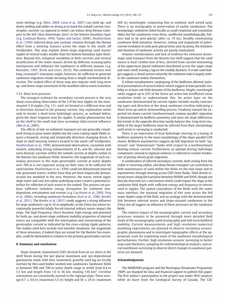
Fig. 20. Paths ofmaximumslope from selected crestline points. Three paths are highlightedwiththe sandwave (trough), generally matching an inflection point in the corresponding profile. Beferred to counter cumulative downslope drift and help maintain sand in the field.

upstream and up-slope recycling is limited, this can only be reconciledwith mobility of the sandwaves that is very slow but this contradictsmost observations.

Establishing a sand budget potentially in balance only demonstratesthat it is possible to generate andmaintain the sands at this location on along-term basis. It dictates a degree of sand mobility yet largely con-fined to field boundaries for long-term maintenance with a minimumflux of sand into and out of the field. Most observations are compatiblewith a dynamic system, more complex than simple feeding, bedformmigration, and exiting of the sands from the fields. Of course, assump-tions of sand source may be incorrect; present up-stream contour-current derived sand flux might be significant and sandwave migrationproportionally active. Future work will address this.

7.3. Possible secondary oceanographic drivers: deep Ekman transporteddies and internal waves?

7.3.1. Long-term processesSecondary processes inferred from the sandwave morphometrics

are best related to relatively constant oceanographic processeswith long term fluctuations or periodicities to which the inherentlyslow-responding large bedforms can tune. For instance, the meso-topographic-related domains in sandwave asymmetry (Figs. 18 and19) representing components of current reversal, the requirementfor long-term sand recycling, and the inferred up-slope sand trans-port component (from ripples) might be explained by the cumulativeand/or combined effect of such processes, even if episodic. Potentialinfluencing processes could be seasonal (winter) downwelling (as sug-gested in Rebesco et al., 2013), seasonal eddies, meandering of theisobath current, or deep Ekman rotation. Some elaboration follows.

Slope-situated topographic perturbations, such as the GDF chutes,would have similar cross-isobath effects on currents as those producedby small canyons, depending on their size. Modeling of canyon-effect in

teepest Paths

583 m depth

cres

t

cres

ttroug

h

2

bathymetric profiles (insert). Most paths showan abrupt directional change at the base oflow the inflection the regional slope is about 1°. A periodic up-slope sand transport is in-


some settings (e.g. Allen, 2004; Lima et al., 2007) can yield up- anddown-welling and eddies so strong as tomask the isobath current. Geo-strophic currents (as opposed to wind) can induce deep Ekman trans-port to the left (thus downslope, here) in the bottom boundary layer(e.g. Cushman-Roisin, 1994; Taylor and Sarkar, 2008). Heathershawet al. (1998) inferred deep anti-cyclonic rotation through the Ekmaneffect from a mooring transect across the slope to the south, offVestfjorden. This may explain down-slope migrating sand waves/ripples of vertical scales smaller than the bottom boundary layer thick-ness. Beyond this, temporal variability in both currents and verticalstratification of the water masses driven by different oceanographicmechanisms will influence the sandwaves in different seasons (e.g.Ramsden, 1995; Brink and Lentz, 2010). The combined vectors overlong (seasonal?) timespans might, however, be sufficient to generatesandwave migration trends deviating from a simple northwesterly di-rection. The seabed effect of these may also migrate with long-termup- anddown-slopemovement of the stratified cold towarm transition.

7.3.2. Short-term processesThe strongest evidence for secondary current process is the very

sharp crosscutting observation of the 2-D lee-face ripples on the stoss-situated 3-D ripples (Fig. 13); each set formed at a different time andat directions normal to the primary current. Any explanation needsonly to invoke a short-term hydrologic process, as outlined below,given the short response time for ripples. A similar phenomenon, buton the shelf to the south had clear secondary tidal current influence(Bøe et al., 2009).

The effects of tide on sediment transport are not generally consid-ered strong at great water depths but the cross-cutting ripple fields re-quire a frequent, strong and temporally direction-changing driver. Aslope to shelf mooring transect located to the south (off Vestfjorden,Heathershaw et al., 1998) demonstrated observations, consistent withmodels, indicating strong enhancements of K2 and M2 (diurnal andsemi-diurnal) currents within the isobath current at depths similar tothe Barents Sea sandwave fields. However, the magnitude of such sec-ondary processes to the main geostrophic current at water depthsover 700 m is not expected, acting on their own, to be sufficient forsand traction. Heathershaw et al. (1998) could not demonstrate internaltide-generated waves; neither have they yet been empirically demon-strated nor modeled in the area. However, the warm, mixed upperslopewater and cool, less saline underlyingwater creates a potential in-terface for reflection of such waves to the seabed. This process can pro-duce sufficient turbulent energy dissipation for sediment non-deposition, entrainment and erosion (e.g. Cacchione et al., 2002; Puiget al., 2004), including sandwave formation (Karl et al., 1986; Reederet al., 2011). The Reeder et al. (2011) study suggests a strong influencefor large sandwaves (up to 16m amplitude) in the China Sea where ex-ceptionally powerful tidally forced internal solitary waves impact theslope. The high frequency–short duration, high energy and potentialfor both up- and down-slope sediment mobility properties of internalwaves are compatible with the interruption and overprinting of thegeostrophic current as indicated by the cross-cutting ripple patterns.The studies cited here include end-member situations; the magnitudeof these processes, if indeed they are extant for the Barents Sea exam-ples, could be diminished in relation to the primary geostrophic current.

8. Summary and conclusions

Slope-situated, channelized GDFs derived from an ice sheet at theshelf break during the last glacial maximum and syn-depositionalglacimarine muds with thin, winnowed, gravelly sand lag are locallyoverlain by thin sand bodies worked into sandwaves. Sandwave fieldsat between 500 and 700 m water depth range in width from 0.4 to3.5 km and length from 1.6 to 36 km, totaling 130 km2. Crestlineorientations are consistently normal to the regional slope. These aver-age 0.7 ± 0.6 m (maximum 5.5 m) height and 58 ± 24 m (maximum

205 m) wavelength, comprising fine to medium, well sorted sand.There is no stratigraphy or preservation of earlier sandwaves. Thehemipelagic sediments failed locally as small rotational and translationslides but the sandwaves cross these, unaffected morphologically. Fail-ures had to be post-glacial (after ca. 15 ka), broadly constrainingsandwave field initiation. However, timing and magnitude of paleo-current evolution in early post-glacial times and, by proxy, the initiationand duration of sandwave activity are poorly constrained.

Volume considerations and lack of evidence for extensive down-slope sand transport from the Barents Sea shelf suggest that the sandsource is local (within tens of km), derived from current winnowingof the uppermost glacial sediments distributed across the upper slopeand outer shelf, leaving a lag on themuddy diamicts. A crude sand bud-get suggests a closed systemwhereby the sediment sink is largely with-in the sandwave bodies themselves.

A robust morphometric cataloguing of the bedforms allowed statis-tical presentations of several indiceswhich suggest at least periodicmo-bility in at least sub-field domains of the bedforms. Height–wavelengthratios suggest up to 25% of the forms are active but insufficient sonarresolution tends to underestimate this. An active layer on thesandwaves demonstrated by current ripples includes starkly contrast-ing types and direction at the sharp sandwave crestline indicating ashort-term up-and/or downwelling process. Tendency toward the ex-pected net down-current (northwestward, contour-parallel) migrationis demonstrated by bedform symmetry and stoss–lee slope differencesbut trends in the opposite direction nearly balance this. Long-termmo-bility of the larger bedforms must be inferred from their morphologyuntil serial re-surveying is conducted.

There is an expression of local hydrologic steering in a tuning ofbedform symmetry to the meso-morphology of the slope-parallel GDFchutes. Bedform asymmetries suggest up-hill migration on both “up-stream” and “downstream” flanks with respect to a northwestwardflowing contour current. Furthermore, an upslope driving hydrologiccomponent (normal to regional contours) is inferred to counter tenden-cies of gravity-driven grain migration.

A combination of inferred secondary currents, both arising from thestable or recurring eddies, and deep Ekman transport can contribute toboth maintenance of sand within the fields on the mid-slope and toasymmetries through steering across GDF chute flanks. Tidal-driven in-ternalwaves along the transition betweenNSAIWandNAW, though notdirectly observed are a mechanismwhich could impact the slope at thesandwave field depth with sufficient energy and frequency to entrainsand in ripples. The spatial coincidence of the fields with the watermass interface, the seasonal migration of this zone across the fullwater depth range of the field, and an analogy with the demonstratedlink between internal waves and slope-situated sandwaves in theChina Sea all suggest an influence of these processes on the sandwavefields.

The relative impact of the oceanographic current and secondaryprocesses remains to be answered through more detailed fieldstudy of the oceanography, sand stratigraphy andmid-term bedformmobility. Current measurements and high resolution numericalmodeling experiments are planned to observe secondary oceano-graphic phenomena and to investigate topographic effects at the ap-propriate scale for explaining some of the sandwave morphologicalperturbations. Further, high resolution acoustic surveying to bettermap sand thickness, sampling for sedimentological analyses, and se-rial multibeam surveying to observe direct changes in sandwave pat-terns are planned.

Acknowledgments

TheMAREANO program and the Norwegian Deepwater Programme(NDP) are thanked for data and financial support to publish this paper.The first author's participation in the project was under NGU auspiceswhile on leave from the Geological Survey of Canada. The GSC


subsequently provided latitude for manuscript preparation in supportof related goals on the Canadian margin. Benedicte Ferre is affiliatedwith the Centre of Excellence: Arctic Gas hydrate, Environment andClimate (CAGE) funded by the Norwegian Research Council (grant no.223259). Michael Li, GSC-Atlantic, provided initial review. Jan SverreLaberg, University of Tromsø and Adriano Viana, Petrobras kindly con-tributed to a better focus on the processes,manuscript clarity and atten-tion to details with their reviews.

References

Allen, J.R.L., 1980. Sand waves: a model of origin and internal structure. SedimentaryGeology 26, 281–328.

Allen, S.E., 2004. Restrictions on deep flow across the shelf-break and the role of subma-rine canyons in facilitating such flow. Surveys in Geophysics 25, 221–247.

Amos, C.L., King, E.L., 1984. Bedforms of the Canadian eastern seaboard: a comparisonwith global occurrences. Marine Geology 57, 167–208.

Andreassen, K., Laberg, J.S., Vorren, T.O., 2008. Seafloor geomorphology of the SW BarentsSea and its glaci-dynamic implications. Geomorphology 97, 157–177.

Ashley, G.M., 1990. Classification of large-scale subaqueous bedforms: a new look at anold problem. Journal of Sedimentary Research 60, 161–172.

Baraza, J., Ercilla, G., Nelson, C.H., 1999. Potential geological hazards on the eastern Gulf ofCadiz slope (SW Spain). Marine Geology 155, 191–215.

Belderson, R.H., Johnson, M.A., Kenyon, N.H., 1982. Bedforms. In: Stride, A.H. (Ed.), Off-shore Tidal Sands: Processes and Deposits. Chapman & Hall, London, pp. 27–57.

Bellec, V.K., Wilson, M., Bøe, R., Rise, L., Thorsnes, T., Buhl-Mortensen, L., Buhl-Mortensen,P., 2008. Bottom currents interpreted from iceberg ploughmarks revealed bymultibeam data at Tromsøflaket, Barents Sea. Marine Geology 249, 257–270.

Bellec, V., Picard, K., Bøe, R., Thorsnes, T., Rise, L., Dolan, M., Elvenes, S., Lepland, A.,Hansen, O.H., 2012a. Geologisk havbunnskart, Kart 71301600, September 2012. M1: 100 000. Norges geologiske undersøkelse. http://www.ngu.no/no/hm/Kart-og-data/Maringeologiske-kart/havbunn-nedlasting/#Ferdige).

Bellec, V., Picard, K., Bøe, R., Thorsnes, T., Rise, L., Dolan, M., Elvenes, S., Lepland, A.,Hansen, O.H., 2012b. Geologisk havbunnskart, Kart 71001600, September 2012. M1: 100 000. Norges geologiske undersøkelse. http://www.ngu.no/no/hm/Kart-og-data/Maringeologiske-kart/havbunn-nedlasting/#Ferdige).

Blindheim, J., Rey, F., 2004. Water-mass formation and distributions in the Nordic Seasduring the 1990s. ICES Journal of Marine Science 61, 846–863.

Bøe, R., Bellec, V.K., Dolan, M.F.J., Buhl-Mortensen, P.B., Buhl-Mortensen, L., Rise, L., 2009.Giant sand waves in the Hola glacial trough off Vesterålen, North Norway. MarineGeology 267, 36–54.

Bøe, R., Bellec, V., Thorsnes, T., Picard, K., Dolan, M., Rise, L., 2010. Tromsøflaket ogEggakanten. In: Buhl-Mortensen, L., Hodnesdal, H., Thorsnes, T. (Eds.), Til bunns iBarentshavet og havområdene utenfor Lofoten - ny kunnskap fra MAREANO forøkosystembasert forvaltning. Norges Geologiske Undersøkelse, Trondheim, Norway,pp. 27–35 (128 pp. (English summary)).

Brink, K.H., Lentz, S.J., 2010. Buoyancy arrest and bottom Ekman transport. Part II: oscillat-ing flow. Journal of Physical Oceanography 40, 636–655.

Buhl-Mortensen, P.B., Buhl-Mortensen, L., Dolan, M., Dannheim, J., Kröger, K., 2009. Mega-faunal diversity associated with marine landscapes of northern Norway: a prelimi-nary assessment. Norwegian Journal of Geology 89, 163–171.

Buhl-Mortensen, L., Hodnesdal, H., Thorsnes, T., 2010. Til bunns i Barentshavet oghavområdene utenfor Lofoten - ny kunnskap fra MAREANO for økosystembasertforvaltning. Norges Geologiske Undersøkelse, Trondheim, Norway (128 pp. (Englishsummary)).

Buhl-Mortensen, L., Bøe, R., Dolan, M.F.J., Buhl-Mortensen, P.B., Thorsnes, T., Elvenes, S.,Hodnesdal, H., 2012. 51 — banks, troughs, and canyons on the continental marginoff Lofoten, Vesterålen, and Troms, Norway. In: Peter, T.H., Elaine, K.B. (Eds.), SeafloorGeomorphology as Benthic Habitat. Elsevier, London, pp. 703–715.

Cacchione, D.A., Pratson, L.F., Ogston, A.S., 2002. The shaping of continental slopes by in-ternal tides. Science 296, 724–727.

Courtney, R., 2007. Storage and dissemination of SEGY Data in JPEG2000 format.American Geophysical Union, Fall Meeting abstract #IN51B-0402.

Cushman-Roisin, B., 1994. Introduction to Geophysical Fluid Dynamics. Englewood Cliffs,N.J., Prentice Hall.

Damuth, J.E., 1980. Use of high-frequency (3.5–12 kHz) echograms in the study of near-bottom sedimentation processes in the deep-sea: a review. Marine Geology 38, 51–75.

Dolan, M., Mortensen, P.B., Thorsnes, T., Buhl-Mortensen, L., Bellec, V.K., Bøe, R., 2009. De-veloping seabed nature-type maps offshore Norway: initial results from theMAREANO programme. Norwegian Journal of Geology 89, 17–28.

Dyer, K.R., 1986. Coastal and Estuarine Sediment Dynamics. Wiley & Sons, Chichester,England.

Ferré, B., Mienert, J., Feseker, T., 2012. Ocean temperature variability for the past 60 yearson the Norwegian–Svalbard margin influences gas hydrate stability on human timescales. Journal of Geophysical Research 117 (C10017).

Flemming, B.W., 1980. Sand transport and bedform patterns on the continental shelfbetween Durban and Port Elizabeth (southeast African continental margin).Sedimentary Geology 26, 179–205.

Habgood, E.L., Kenyon, N.H., Masson, D.G., Akhmetzhanov, A., Weaver, P.P.E., Gardner, J.,Mulder, T., 2003. Deep-water sediment wave fields, bottom current sand channelsand gravity flow channel-lobe systems: Gulf of Cadiz, NE Atlantic. Sedimentology50, 483–510.

Hald, M., Vorren, T.O., 1984. Modern and Holocene foraminifera and sediments on thecontinental shelf off Troms, North Norway. Boreas 13, 133–154.

Hanquiez, V., Mulder, T., Lecroart, P., Gonthier, E., Marchès, E., Voisset, M., 2007. High res-olution seafloor images in the Gulf of Cadiz, Iberian margin. Marine Geology 246,42–59.

Hansen, B., Østerhus, S., 2000. North Atlantic-Nordic Seas exchanges. Progress in Ocean-ography 45 (2), 109–208.

Haugan, P.M., Evensen, G., Johannessen, J.A., Johannessen, O.M., Pettersson, L.H., 1991.Modeled and observed mesoscale circulation and wave-current refraction duringthe 1988 Norwegian continental shelf experiment. Journal of Geophysical Research96 (C6), 10487–10506.

Heathershaw, A.D., Hall, P., Huthnance, J.M., 1998. Measurements of the slope current,tidal characteristics and variability west of Vestfjorden, Norway. Continental Shelf Re-search 18, 1419–1453.

Heezen, B.C., Hollister, C.D., 1971. The Face of the Deep. Oxford University Press,New York.

Helland-Hansen, B., Nansen, F., 1909. The Norwegian sea: its physical oceanographybased upon Norwegian researches 1900–1904. Report on Norwegian Fishery andMarine investigations. , vol. II 1909 Mo. 2. Det Mallingske bogtrykkeri, Kristiania(390 pp.).

Hopkins, T.S., 1991. The GIN Sea— a synthesis of its physical oceanography and literaturereview 1972–1985. Earth-Science Reviews 30, 175–318.

Karl, H.A., Cacchione, D.A., Carlson, P.R., 1986. Internal-wave currents as a mechanism toaccount for large sand waves in Navarinsky Canyon Head, Bering Sea. Journal ofSedimentary Petrology 56, 706–714.

Kenyon, N.H., 1986. Evidence from bedforms for a strong poleward current along theupper continental slope of northwest Europe. Marine Geology 72, 186–198.

Kenyon, N.H., Belderson, R.H., 1973. Bedforms of the Mediterranean undercurrent ob-served with sidescan sonar. Sedimentary Geology 9, 77–99.

King, E.L., Sejrup, H.P., Haflidason, H., Elverhøi, A., Aarseth, I., 1996. Quaternary seismicstratigraphy of the North Sea Fan: glacially-fed gravity flow aprons, hemipelagicsediments, and large submarine slides. Marine Geology 130, 293–315.

King, E.L., Bøe, R., Bellec, V.K., Rise, L., Dolan, M., 2011. Contour current driven sandwaveson the upper slope of the continentalmargin offshore northern Norway— setting andmorphometrics. NGU Report 2011.073 (93 pp.).

Laberg, J.S., Vorren, T.O., 1993. A Late Pleistocene submarine slide on the Bear IslandTrough Mouth Fan. Geo-Marine Letters 13, 227–234.

Laberg, J.S., Vorren, T.O., 1995. Late Weichselian submarine debris flow deposits on theBear Island Trough Mouth Fan. Marine Geology 127, 45–72.

Laberg, J.S., Vorren, T.O., 2004. Weichselian and Holocene growth of the northern high-latitude Lofoten Contourite Drift on the continental slope of Norway. SedimentaryGeology 164, 1–17.

Laberg, J.S., Vorren, T.O., Knutsen, S.M., 1999. The Lofoten contourite drift off Norway.Marine Geology 159, 1–6.

Laberg, J.S., Andreassen, K., Knies, J., Vorren, T.O., Winsborrow, M., 2010. Late Pliocene–Pleistocene development of the Barents Sea ice sheet. Geology 38 (2), 107–110.

Lima, J.A.M., Möller, O.O., Viana, A.R., Piovesan, R., 2007. Hydrodynamic modelling ofbottom currents and sediment transport in the Canyon São Tomé (Brazil). In:Viana, A.R., Rebesco, M. (Eds.), Geological Society, London, Special Publications, 276,pp. 329–342.

Masson, D.G., 2001. Sedimentary processes shaping the eastern slope of the Faeroe–Shetland Channel. Continental Shelf Research 21, 825–857.

Michels, K.H., 2000. Inferring maximum geostrophic current velocities in the Norwegian–Greenland Sea from measurements of sediment surface samples: methods, applica-tion, and results. Journal of Sedimentary Research 70, 1036–1050.

Mork, K.A., Skagseth, O., 2010. A quantitative description of the Norwegian Atlantic Cur-rent by combining altimetry and hydrography. Ocean Science 6 (4), 901–911.

Mulder, T., 2003. Deep-water sediment wave fields, bottom current sand channels andgravity flow channel-lobe systems: Gulf of Cadiz, NE Atlantic. Sedimentology 50,483–510.

Nygård, A., Sejrup, H.P., Haflidason, H., King, E.L., 2002. Geometry and genesis of glacigenicdebris flows on the North Sea Fan: TOBI imagery and deep-tow boomer evidence.Marine Geology 188, 15–33.

Ottesen, D., Dowdeswell, J.A., Rise, L., 2005. Submarine landforms and the reconstructionof fast-flowing ice streams within a large Quaternary ice sheet: the 2,500 km-longNorwegian–Svalbard margin (57°–80° N). Geological Society of America Bulletin117, 1033–1050.

Poulain, P.-M., Warn-Varnas, A., Niiler, P.P., 1996. Near-surface circulation of the Nordicseas as measured by Lagrangian drifters. Journal of Geophysical Research 101,237–258.

Puig, P., Palanques, A., Guillén, J., El Khatab, M., 2004. Role of internal waves in the gener-ation of nepheloid layers on the northwestern Alboran slope: implications for conti-nental margin shaping. Journal of Geophysical Research 109 (C09011).

Ramsden, D., 1995. Response of an oceanic bottom boundary-layer on a slope to interiorflow.1. Time-independent interior flow. Journal of Physical Oceanography 25,1672–1687.

Rebesco, M., Wåhlin, A., Laberg, J.S., Schauer, U., Beszczynska-Möller, A., Lucchi, R.G.,Noormets, R., Accettella, D., Zarayskaya, Y., Diviacco, P., 2013. Quaternary contouritedrifts of the Western Spitsbergen margin. Deep-Sea Research Part I 156–168.

Reeder, D.B., Ma, B.B., Yang, Y.J., 2011. Very large subaqueous sand dunes on the uppercontinental slope in the South China Sea generated by episodic, shoaling deep-water internal solitary waves. Marine Geology 279, 12–18.

Rubin, D.M., McCulloch, D.S., 1980. Single and superimposed bedforms: a synthesis of SanFrancisco Bay and flume observations. Sedimentary Geology 26, 207–231.

Rudels, B., Friedrich, H.J., Quadfasel, D., 1999. The Arctic circumpolar boundary current.Deep Sea Research Part II: Topical Studies in Oceanography 46 (6–7), 1023–1062.

http://refhub.elsevier.com/S0025-3227(14)00089-9/rf0010
















http://www.ngu.no/no/hm/Kart-og-data/Maringeologiske-kart/havbunn-nedlasting/#Ferdige




































































































































Schlitzer, R., 2012. Ocean Data View. http://odv.awi.de.Ślubowska-Woldengen, M., Koç, N., Rasmussen, T.L., Klitgaard-Kristensen, D., Hald, M.,

Jennings, A.E., 2008. Time-slice reconstructions of ocean circulation changes on thecontinental shelf in the Nordic and Barents Seas during the last 16,000 cal yr BP. Qua-ternary Science Reviews 27, 1476–1492.

Taylor, J.R., Sarkar, S., 2008. Stratification effects in a bottom Ekman layer. Journal ofPhysical Oceanography 38, 2535–2555.

Viana, A.R., Faugères, J.-C., Stow, D.A.W., 1998a. Bottom-current-controlled sand deposits—a review of modern shallow- to deep-water environments. Sedimentary Geology 115,53–80.

Viana, A.R., Faugères, J.-C., Kowsmann, R.O., Lima, R.O., Caddah, J.A.M., Rizzo, J.G., 1998b.Hydrology, morphology and sedimentology of the Campos continental margin, off-shore Brazil. In: Stow, D.A.W., Faugères, J.-C. (Eds.), Contourites, Turbidites and Pro-cess Interaction. Sedimentary Geology, 115, pp. 133–157.

Vorren, T.O., Hald, M., Thomsen, E., 1984. Quaternary sediments and environments on thecontinental shelf off northern Norway. Marine Geology 57, 229–257.

Vorren, T.O., Lebesbye, E., Andreassen, K., Larsen, K.-B., 1989. Glacigenic sediments on apassive continental margin as exemplified by the Barents Sea. Marine Geology 85,251–272.

Vorren, T.O., Laberg, J.S., Blaume, F., Dowdeswell, J.A., Kenyon, N.H., Mienert, J., Rumohr, J.,Werner, F., 1998. The Norwegian–Greenland Sea continental margins: morphologyand late Quaternary sedimentary processes and environment. Quaternary ScienceReviews 17, 273–302.

Winsborrow, M.C.M., Andreassen, K., Corner, G.D., Laberg, J.S., 2010. Deglaciation of amarine-based ice sheet: late Weichselian palaeo-ice dynamics and retreat in thesouthern Barents Sea reconstructed from onshore and offshore glacial geomorpholo-gy. Quaternary Science Reviews 29, 424–442.

Wynn, R.B., Stow, D.A.V., 2002. Classification and characterisation of deep-water sedimentwaves. Marine Geology 192, 7–22.

Wynn, R.B., Masson, D.G., Stow, D.A.V., Weaver, P.P.E., 2000. Turbidity current sedimentwaves on the submarine slopes of the western Canary Islands. Marine Geology 163,185–198.

http://odv.awi.de





























Documents

Contour current driven continental slope-situated sandwaves with effects from secondary current processes on the Barents Sea margin offshore Norway