Continuum Model for the Phase Behavior, Microstructure, andRheology of Unentangled Polymer Nanocomposite MeltsPavlos S. Stephanou,*,† Vlasis G. Mavrantzas,‡,§ and Georgios C. Georgiou†

†Department of Mathematics and Statistics, University of Cyprus, PO Box 20537, 1678 Nicosia, Cyprus‡Department of Chemical Engineering, University of Patras & FORTH-ICE/HT, Patras, GR 26504, Greece§Department of Materials, Polymer Physics, ETH Zurich, HCI H 543, CH-8093 Zurich, Switzerland

*S Supporting Information

ABSTRACT: We introduce a continuum model for polymer melts filled withnanoparticles capable of describing in a unified and self-consistent way theirmicrostructure, phase behavior, and rheology in both the linear and nonlinearregimes. It is based on the Hamiltonian formulation of transport phenomena forfluids with a complex microstructure with the final dynamic equations derived bymeans of a generalized (Poisson plus dissipative) bracket. The model describesthe polymer nanocomposite melt at a mesoscopic level by using three fields (statevariables): a vectorial (the momentum density) and two tensorial ones (theconformation tensor for polymer chains and the orientation tensor fornanoparticles). The dynamic equations are developed for nanoparticles with anarbitrary shape but then they are specified to the case of spherical ones.Restrictions on the parameters of the model are provided by analyzing itsthermodynamic admissibility. A key ingredient of the model is the expression forthe Helmholtz free energy A of the polymer nanocomposite. At equilibrium this reduces to the form introduced by Mackay et al.(Science 2006, 311, 1740−1743) to explain the phase behavior of polystyrene melts filled with silica nanoparticles. Beyondequilibrium, A contains additional terms that account for the coupling between microstructure and flow. In the absence of chainelasticity, the proposed evolution equations capture known models for the hydrodynamics of a Newtonian suspension ofparticles. A thorough comparison against several sets of experimental and simulation data demonstrates the unique capability ofthe model to accurately describe chain conformation and swelling in polymer melt nanocomposites and to reliably fit measuredrheological data for their shear and complex viscosity over large ranges of volume fractions and deformation rates.

I. INTRODUCTION

Composite or heterogeneous materials can be found inabundance in nature. Two simple, nature-produced, polymer-based examples are wood (made up of fibrous chains ofcellulose in a matrix of lignin) and bone (composed of hardinorganic crystals, hydroxyapatite, embedded in an organicmatrix of collagen).1 These materials find numerousapplications in electronics, optics, catalysis, ceramics, andmagnetic data storage devices.2 Their widespread applications(from bulletproof vests to golf clubs, from vehicle tires tomissile parts, etc.) has certainly integrated them into our lives.3

Polymer matrix nanocomposites (PNCs), in particular, arehybrid organic/inorganic composites formed by the addition ofnanoparticles to a polymer matrix, and blood and paint are onlytwo of the numerous examples that demonstrate theirimportance.4 Recent applications include use in solar photo-voltaic devices,5 in the development of lightweight materials forelectrical applications,6 and in diagnostics and therapy (e.g., asdrug carriers to fight cancer7). At least one of the dimensions ofthe filler phase is in the nanometer scale leading to a largeinterfacial contact area with neighboring polymer chains. As aresult, the composite material can have significantly improvedproperties relative to the pure polymer even at extremely small

volume fractions (loadings) of the filler, and this has renewedinterest in these systems in the past few years. Low-volumeadditions (1−10%) of isotropic (e.g., titania, alumina, andsilver) or anisotropic (e.g., layered silicates, carbon nanotubesand nanofibers) nanoparticles result in significantly improvedproperties, comparable to those achieved via conventionalloading (15−40%) of micrometer-scale inorganic fillers.8

Materials with a variety of shapes may be employed as fillersin PNCs, such as nanoclays (primarily polymer-layered silicates,PLS),9,10 nanoscopic silica particles,9,11 nanotubes,12 nano-fibers,13 and many others. This justifies the large number ofsimulation studies,14,15 theories,16 and rheological measure-ments17 that have appeared recently in an effort to explainproperties of this important class of materials and tounderstand fundamental issues related to chain dynamics inthe vicinity of nanoparticle surface,18,19 entanglement anddisentanglement effects via primitive path analysis,20,21 meltrheology,22,23 and the importance of energetics and cluster-ing.24

Received: February 25, 2014Revised: May 23, 2014Published: June 19, 2014

Article

pubs.acs.org/Macromolecules

© 2014 American Chemical Society 4493 dx.doi.org/10.1021/ma500415w | Macromolecules 2014, 47, 4493−4513

From the point of view of industrial applications, the interestlies in the rheological behavior of PNCs, with an emphasis onthe dependence of the key material functions (shear viscosity,first and second normal stress coefficients, storage and lossmoduli) on shear rate and nanoparticle volume fraction. Thecelebrated equation of Einstein25 for the relative viscosity,namely ηr = η/η0 = 1 + (5/2)ϕ, where η denotes the viscosityof the suspension, η0 the viscosity of the solvent, and ϕ thenanoparticle volume fraction, has been shown to accuratelydescribe the rheological behavior of Newtonian sphericalsuspensions at low volume fractions (ϕ ∼ 0.02), providedinterparticle interactions are neglected. Batchelor and Green26

extended Einstein’s equation to higher volume fractions (ϕ ∼0.1) by considering the effect of pairwise interactions and thusderiving the second-order term in the expansion of ηr withrespect to ϕ; this correction has been verified experimentally.27

Einstein’s expression was extended to spheroids by Jeffery28

who showed that the effective viscosity depends on particleorientation, namely ηr = 1 + Cϕ, where C is a numericalparameter whose value depends on whether the spheroid isoblate or prolate. Hinch and Leal29 computed an ensemble-averaged effective viscosity by including effects due to rotationaldiffusion. A general theory for dilute particle suspensions wasput forth by Batchelor and Brenner.30

Most of the above hydrodynamic theories are limited tosmall volume fractions. Experimental data show that eventuallythe relative viscosity diverges at a volume fraction commonlydenoted as the maximum packing fraction ϕT, whichexperimentally is found to lie in the range 0.55−0.71 [see,e.g., ref 31]. To account for this, simple empirical extensionshave been proposed that employ a 1 − (ϕ/ϕT) term in thedenominator. Such equations will be discussed later in thisarticle.For PNCs, the situation is more complicated: experimental

observations fail to provide a satisfactory picture of theirrheological behavior. Although early observations were in favorof an increased viscosity relative to the pure polymer,32

evidence has been accumulated recently pointing (in manycases) to a reduced viscosity for PNCs when filled withspherical particles, which is unique only to this type ofnanosized fillers. In particular, when fullerenes are added tomonodisperse, linear, high molecular weight polysterene, theviscosity decreases,33 an effect which has been attributed to thethermodynamic stability of the dispersion (this is attained onlywhen the size of the fullerenes is smaller than the radius-of-gyration Rg of the polymer chains). The phenomenon seems tobe connected with entanglement effects, since unentangled ornearly entangled systems (characterized by molecular weightMmw ∼ Mc, where Mc is the critical molecular weight at whichentanglement effects become important) exhibit an increasedzero shear rate viscosity when nanoparticles are added; incontrast, samples withMmw exceedingMc exhibit a reduced zeroshear rate viscosity. Initially, this decrease was postulated to berelated to the increase in the free volume of the melt caused bythe addition of nanoparticles but later such an explanation wasruled out. According to Tuteja et al.,33 the viscosity η0 willdecrease when (a) polymer chains are long enough to beentangled and (b) the average distance between nanoparticles issmaller than twice the polymer Rg. Additional experimentalstudies on poly(propylene) showed a similar decrease in theviscosity when silica nanoparticles were introduced into thematrix, which was attributed to the selective adsorption of highmolecular weight polymer chains on the surface of silica.34

Wang and Hill35 explained this behavior by proposing (in theframework of a continuum hydrodynamic model) that in aPNC melt, a polymeric layer is formed in the neighborhood ofthe nanoparticle characterized by a smaller viscosity than thebulk polymer; the model, however, suffers from the assumptionthat the polymer matrix behaves as a Newtonian fluid.Needeless to say that, from a practical point of view, such adecrease in the viscosity would be highly desirable, since itimplies that the processability of the material will be enhanced.Starr et al.36 have shown that the glass transition temperature

Tg of a polymer melt can be shifted to either higher or lowertemperatures by tuning the interactions between polymer andfiller. The relaxation time of the radially averaged intermediatescattering function of the filled system should be larger thanthat of the unfilled one when the polymer−nanoparticleinteractions are attractive (implying an increased Tg) butshould decrease when the interactions are nonattractive(implying a decreased Tg).

36 The increase in relaxation time,which has also been observed in recent molecular dynamics(MD) simulations,37 has been reported to be exponential.15

From the processing point of view, in addition to Tg, anotherimportant issue is that of miscibility, i.e., of the properdispersion of nanoparticles in the polymeric matrix. Theoreticalwork by Hooper and Schweizer38 has revealed two distinctspinodal curves: one at low nanoparticle−monomer attractionstrengths associated with the formation of a thermodynamicallystable polymer layer around nanoparticles (this is insensitive tonanoparticle size asymmetry ratio D/bd with D and bd denotingthe nanoparticle diameter and monomer diameter or bead size,respectively) and a second one at higher attraction strengthsassociated with the formation of thermodynamically stablebridges as polymer segments connect different nanoparticles(this is more sensitive to the ratio D/bd). The two spinodalcurves are separated by a “miscibility window”. Thesetheoretical findings have also been confirmed by recent MDsimulations.39 The proper dispersion of spherical nanoparticlesis typically associated with polymer swelling (the increase in thedimensions of polymer chains when nanoparticles areintroduced in the polymer matrix).34 This further motivatedMackay et al.40 to propose a modified Flory−Huggins theory todescribe the experimental findings.Despite ample experimental41 and simulation15,18,21 evidence

that the addition of nanoparticles induces polymer swelling,Crawford et al.42 found that the ratio Rg/Rg0 (where Rg0 denotesthe chain radius-of-gyration of the unfilled polymer) remainsclose to unity even up to ϕ ∼ 0.35. However, these authorshave shown that for Rg ≤ a (a = D/2) PNCs phase separatewhereas for Rg>a a uniform dispersion should be obtained.Given that similar Rg/a ratios were used, the disagreement oftheir study with previous works [e.g., that of ref 40] suggeststhat polymer size may not be the only relevant parametercontrolling chain swelling.As far as the nonlinear rheology of PNCs is concerned, the

works of Anderson and Zukoski43,44 and Zhang and Archer45

have shown that, following the linear viscoelastic (LVE)plateau, polymers filled with spherical nanoparticles exhibit ashear thinning behavior as the shear rate increases. Shearthinning occurs when hydrodynamic stresses prevail overthermodynamic ones,43 resulting in a fast reduction of theviscosity with shear rate. By further increasing the shear rate,the viscosity curves for different volume fractions approachmore and more that of the pure polymer. At very large shearrates, finally, the viscosity curves approach a plateau (an infinite

Macromolecules Article

dx.doi.org/10.1021/ma500415w | Macromolecules 2014, 47, 4493−45134494

shear rate viscosity).43 A similar shear-thinning behavior hasbeen reported in the case of polymer melts filled withnanoclays46 and nanofibers.47

In network theories,48 physical entanglements betweenchains are considered as junctions between segments whichmay be destroyed and later recreated. Doremus and Piau49

realized that the addition of nanoparticles would induceadditional junctions due to adsorption of portions of chainson nanoparticles. Thus, a double network should emerge withdifferent creation and destruction probabilities for each of thepolymer−polymer and polymer−nanoparticle segments.50 Asimilar double network approach has been adopted bySarvestani and Picu51 who derived expressions for the ratesof chain attachment to and detachment from the nanoparticle;in a subsequent study, they used these expressions to introducemodifications to the friction coefficient of an encapsulatedFENE dumbbell. Another kinetic theory approach was that ofXu et al.52 where elastic dumbbells (being isotropic oranisotropic, with or without hydrodynamic interactions) wereused to model nanofiber suspensions. It turns out that severalauthors53 have proposed modifications to the reptation timedue to chain attachment-detachment in the presence ofnanoparticles.In a number of more recent papers, Grmela and co-workers

employed the GENERIC54,55 formalism of nonequilibriumthermodynamics (NET) to describe the rheology ofPNCs.56−58 To model polymer chains they used theconformation tensor C while for the orientation of the fibersthey employed a constrained (to reflect the constant length offibers) orientation tensor a (both of these tensors will bediscussed in due detail in the next section). Grmela and co-workers also made attempts to model nanoclay PNCs initiallywith the FENE-P model56,57 and later by explicitly consideringreptating chains.46,58 To the best of our knowledge and despiteseveral nonequilibrium thermodynamics studies of polymer−nanofiber and polymer−nanoclay systems, there has been nowork addressing the case of polymer nanocomposite melts withnanospheres.In this work, we introduce a rheological model for PNCs

with spherical nanoparticles in the context of the generalizedbracket formalism of NET,59 by means of which several systems(primarily liquid crystals and polymers) and phenomena (suchas polymer-wall interactions and polymer diffusion due to stressgradients in inhomogeneous flow fields) have been successfullyaddressed over the years.55,59 Our approach (as well as that ofGrmela and co-workers based on GENERIC) has theadvantage that the final equations are developed in the contextof a formalism which guarantees consistency with the first andsecond law of thermodynamics. In addition, it is very systematic(offering a unified description of phase behavior, transportphenomena and rheology) and can easily be coupled with amicroscopic model for the underlying molecular interactionsallowing for the full parametrization of the model. For practicalapplications, this is actually also the major disadvantage of themodel, since it shows that it is not autonomous: for thecomplete description of the problem, additional input isrequired from lower-level simulations or models. We mention,for example, the expression for the free energy which should beindependently derived from a microscopic model. Our aim inthis study is ultimately to generalize our recent rheologicalmodel for homopolymers,60,61 which has proven quite accuratein describing the results of direct atomistic non-equilibriummolecular dynamics (NEMD) simulations60,61 and thermody-

namically guided simulations at low and moderate shear rates,62

to the more complex case of (unentangled or entangled)polymer matrices containing nanoparticles.The paper is structured as follows: in section II a brief

overview of the generalized bracket formalism of non-equilibrium thermodynamics is given. In section III, the newmodel is introduced: our choice of the state variables isdiscussed, the expression for the extended Helmholtz freeenergy is provided, and the full formulae for the Poisson anddissipation brackets are given. The dynamic equations for thecase of spherical nanoparticles are derived and the modelequations are reduced to known expressions in the limiting caseof spherical particles dispersed in a Newtonian liquid. Alsoincluded in section III is the analysis of the thermodynamicadmissibility of the model and the positive-definiteness of theconformation tensor. In section IV the expressions for therelevant rheological material functions obtained by analyzingthe asymptotic behavior of the model in the limits of smallshear and small uniaxial elongational flows are reported. Insection V, the results obtained with the new model arepresented: we first discuss its parametrization and then weshow how accurately and reliably it can describe availableexperimental and simulation data for the shear viscosity ofseveral PNC melts as a function of nanoparticle volume fractionover a wide range of shear rates. The paper concludes withsection VI where the most important aspects of the new modelare summarized and future plans are discussed.At this point, we clarify that, in this work, (a) we have

restricted ourselves to the case of well-dispersed nanoparticlesin the polymer matrix and (b) we have used Einstein’s implicitsummation convention for any repeated Greek indices. Wehave also tried to keep in the paper only the most importantmaterial (equations and calculations) necessary to follow thepresentation and derivation of the new model leaving technical(mostly mathematical) details for the accompanying Support-ing Information.

II. NON-EQUILIBRIUM THERMODYNAMICSIn the context of classical mechanics, the appropriate set ofstate variables to consider for an N-particle system is x = {r,p}with r = (r1,..,rN) and p = (p1,..,pN), where rj and pj denote theposition and momentum vectors of the jth particle, respectively.Then, the time evolution of an arbitrary functional F isgoverned by Hamilton’s equation of motion:54,55,59,63

=Ft

F Edd

{ , }(1)

where E is the total energy or the Hamiltonian H of the systemand {.,.} denotes the Poisson bracket. These systems are purelyconservative, and the Poisson bracket has the bilinear form

∫ δδ

δδ

= · ·F EF Ex

Lx

r{ , } d3(2)

where L is the Poisson matrix.54,55 The Poisson bracket mustbe antisymmetric {F,G} = −{G,F}, in order for the energy to beconserved, dE/dt = 0. It must also be time invariant and as suchit should satisfy the Jacobi identity {F,{G,P}} + {G,{P,F}} +{P,{F,G}} = 0 for arbitrary functionals F, G and P.54,55 In theliterature, one can find guidelines and rules how to choose thePoisson bracket or, equivalently, the L matrix in order for theJacobi identity to be automatically satisfied.55 In addition, thereis an automated code available online to check the Jacobiidentity.64

Macromolecules Article

dx.doi.org/10.1021/ma500415w | Macromolecules 2014, 47, 4493−45134495

In actual applications, however, it is almost impossible towork with all degrees of freedom of the N-particle system.Instead, it is preferable to keep only a set of few slowly varyingvariables, meaning that fast degrees of freedom are averagedout, a procedure known as coarse-graining. Through such aprocedure irrelevant degrees of freedom are eliminated at theexpense of introducing entropy and dissipation.65 To accountthen for the friction associated with the eliminated fast degreesof freedom, irreversibility must be added to the evolutionequations at the coarse-grained level of description. Even whenwe start from a coarser (than the atomistic) level in whichirreversible contributions have already been considered,additional irreversibility will be born when we will furthercoarse-grain by eliminating extra (fast) degrees of freedom. Atthis (coarse-grained) level of description, the evolution of statevariables is elegantly separated as55,63

= +t t tx x xd

ddd

ddreversible irreversible (3)

with the second contribution given (in a spirit similar to thefirst) as

=Ft

F Sdd

[ , ]irreversible (4)

where S is the system’s total entropy and [.,.] denotes thedissipation bracket. Similar to eq 2, the latter is expressed as

∫ δδ

δδ

= · ·F SF Sx

Mx

r[ , ] df3

(5)

where Mf is the friction matrix54,55 associated with theincreasing number of processes treated as fluctuations uponcoarse-graining to slower and slower variables,64 a directconsequence of the fluctuation−dissipation theorem. Thedissipation bracket must be symmetric [F,G] = [G,F] andpositive semidefinite [F,F] ≥ 0 in order for the evolutionequation(s) to satisfy the second law of thermodynamics (theprinciple of non-negative rate-of-entropy production). Thus, wehave a Poisson matrix L (or a Poisson bracket) that turnsenergy gradients into reversible dynamics and a friction matrixMf (or a dissipation bracket) that turns entropy gradients intoirreversible dynamics. To strictly separate reversible andirreversible contributions, the following mutual degeneracyrequirements are further introduced:54,55

δδδδ

= ⇒ · =

= ⇒ · =

F SS

F EE

Lx

Mx

{ , } 0 0

[ , ] 0 0f (6)

The above conditions express the conservation of energy in thepresence of dissipation and the conservation of entropy for anyreversible dynamics.Closely related to GENERIC is the generalized bracket

approach,59 a one-generator formalism expressed as

= +Ft

F H F Hdd

{ , } [ , ](7)

Except from subtle issues in the case of systems described (e.g.)by the Boltzmann equation66 (i.e., through distributionfunctions) that favor GENERIC, the two formalisms are incomplete agreement,67 and thus may be used interchangeably.

A key issue in all nonequilibrium thermodynamics formal-isms is the choice of state variables.63,65 Althouth this is obviouswhen one deals with structureless media [in which case thestate variables include the mass density ρ, the momentumdensity M (or the velocity u = M/ρ), and the energy density ε(or the entropy density s or the temperature T)], it is an issueof paramount importance when structured media areconsidered because of the additional internal variables thatneed to be considered in order to describe the microstructureof the system.63 It is an issue requiring deep physical intuitionand experience.63 Typical choices for structural variablesinclude a distribution function, the tensor of second momentsof a distribution function, a scalar, etc.

III. GENERALIZED BRACKET BUILDING BLOCKS FORPOLYMER NANOCOMPOSITES

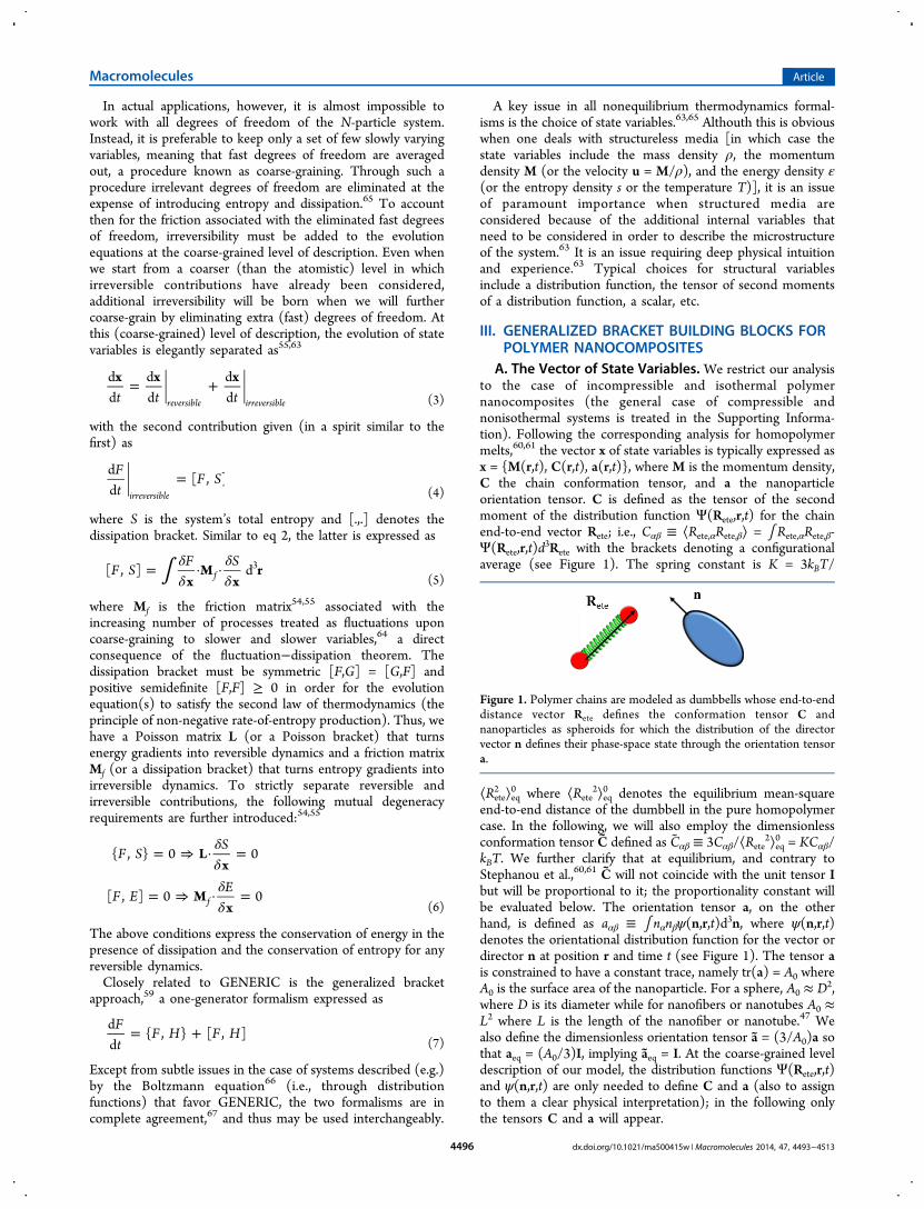
A. The Vector of State Variables. We restrict our analysisto the case of incompressible and isothermal polymernanocomposites (the general case of compressible andnonisothermal systems is treated in the Supporting Informa-tion). Following the corresponding analysis for homopolymermelts,60,61 the vector x of state variables is typically expressed asx = {M(r,t), C(r,t), a(r,t)}, where M is the momentum density,C the chain conformation tensor, and a the nanoparticleorientation tensor. C is defined as the tensor of the secondmoment of the distribution function Ψ(Rete,r,t) for the chainend-to-end vector Rete; i.e., Cαβ ≡ ⟨Rete,αRete,β⟩ = ∫ Rete,αRete,β-Ψ(Rete,r,t)d

3Rete with the brackets denoting a configurationalaverage (see Figure 1). The spring constant is K = 3kBT/

⟨Rete2 ⟩eq

0 where ⟨Rete2⟩eq

0 denotes the equilibrium mean-squareend-to-end distance of the dumbbell in the pure homopolymercase. In the following, we will also employ the dimensionlessconformation tensor C defined as Cαβ ≡ 3Cαβ/⟨Rete

2⟩eq0 = KCαβ/

kBT. We further clarify that at equilibrium, and contrary toStephanou et al.,60,61 C will not coincide with the unit tensor Ibut will be proportional to it; the proportionality constant willbe evaluated below. The orientation tensor a, on the otherhand, is defined as aαβ ≡ ∫ nαnβψ(n,r,t)d3n, where ψ(n,r,t)denotes the orientational distribution function for the vector ordirector n at position r and time t (see Figure 1). The tensor ais constrained to have a constant trace, namely tr(a) = A0 whereA0 is the surface area of the nanoparticle. For a sphere, A0 ≈ D2,where D is its diameter while for nanofibers or nanotubes A0 ≈L2 where L is the length of the nanofiber or nanotube.47 Wealso define the dimensionless orientation tensor a = (3/A0)a sothat aeq = (A0/3)I, implying aeq = I. At the coarse-grained leveldescription of our model, the distribution functions Ψ(Rete,r,t)and ψ(n,r,t) are only needed to define C and a (also to assignto them a clear physical interpretation); in the following onlythe tensors C and a will appear.

Figure 1. Polymer chains are modeled as dumbbells whose end-to-enddistance vector Rete defines the conformation tensor C andnanoparticles as spheroids for which the distribution of the directorvector n defines their phase-space state through the orientation tensora.

Macromolecules Article

dx.doi.org/10.1021/ma500415w | Macromolecules 2014, 47, 4493−45134496

B. The Hamiltonian. For incompressible and isothermalsystems, the Hamiltonian is written as the sum of a kineticenergy Ken and a Helmholtz free energy term A:59 Hm = Ken + A= ∫ (M2/(2ρ)d3r + A. The latter is given here by the followingexpression:

= + + + ‐A A A A Amix pol np pol np (8)

where Amix denotes the free energy of nanoparticle−polymermixing, Apol is the elastic energy of polymer chains, Anp is thefree energy due to nanoparticle orientation, and Apol‑np is thefree energy due to (enthalpic, steric, and topological)interactions between polymer chains and nanoparticles.Free Energy of Mixing. For Amix, we choose the modified

Flory−Huggins expression proposed by Mackay et al.:40

χϕ ϕ ϕ ϕ ϕ ϕ= − + + − −v A

Vk Tt(1 ) ln (1 ) ln(1 )M

np mix

B(9)

where vnp denotes the volume of the nanoparticle, kB theBoltzmann constant, χ the Flory mixing parameter, V thevolume of the sample, ϕ the volume fraction of nanoparticles,and the parameter tM is defined as tM = (D/2Rg0)

3(ρp/ρ0),where Rg0 denotes the chain radius-of-gyration of the neatpolymer at equilibrium, ρp the density of the neat polymer melt,and ρ0 the density of a single polymer chain. Alternatively, theparameter tM can be expressed as tM = vnpρpNav/Mmw =nppure/na

pure, where nppure and na

pure denote the pure nanoparticleand pure polymer number densities, respectively. If ρp denotesthe polymer mass density and Nav is the Avogadro number,then np

pure = ρpNav/Mmw and napure = vnp

−1. Equation 9 accountsfor the Helmholtz free energy of mixing between polymerchains and nanoparticles and is able to describe (see AppendixA) the phase behavior of the nanocomposite in the sense that itcan reproduce the bimodal obtained by Mackay et al.40 Anadditional term called the Carnahan−Starling potentialdescribing the nonideal part of the translational entropy of ahard-sphere gas can also been used,68 but since it does not alterthe phase behavior,40 it will be omitted here. In general, theform of Amix in our model has to be chosen with care, based onintuition and experience for the particular system at hand,because several different forms can be accommodated at our(coarse-grained) level of description.Elastic Energy of Polymer Chains. For Apol we have directly

used the expression provided by Stephanou et al.60,61 with aslight modification:

∫ϕ=

+Φ − ⎧⎨⎩

⎫⎬⎭An K f k T

KC C r

[1 ( )]

2(tr ) ln det dp

polB 3

(10)

Equation 10 describes the total elastic energy of the polymerphase (as such, it is proportional to the polymer chain numberdensity np) with polymer chains modeled as elastic (and, ingeneral, nonlinear) springs with a spring constant K and aspring potential energy function Φ. This term is proportional tof(ϕ), a function which is introduced in order for the theory tobe able to capture Einstein’s equation for the viscosity of aNewtonian suspension of spherical particles. Indeed, with theform of eq 10 for Apol, it turns out that the shear stress in shearflow is given by ταβ = η0[1 + f(ϕ)]γαβ (see section III.H).Therefore, by choosing f(ϕ) = (5/2)ϕ, we recover Einstein’sformula for the reduced viscosity of a Newtonian suspension of

hard spheres. Of course, one may employ any other functionalform for f available from a lower-level theory or experiments.Formally, there are two ways to reproduce Einstein’s

equation for the viscosity of a dilute suspension of nanoparticlesusing the generalized bracket: one is to add to the Hamiltoniana separate kinetic energy term for the particles due to theirtranslational motion; the second is to consider (in addition tothe linear momentum vector) the vorticity vector in the list ofstate variables and specify some additional coupling in thedissipation matrix (see examples 7.3 and 7.5 in ref 59). To keepthe model simple, here we have used a third method: to use amultiplicative factor in the expression for the free energy due topolymer elasticity, implying an effective spring constant forpolymer dumbbells in the presence of nanaparticles equal to theproduct of K with the function f(ϕ).As far as the −ln det C term in eq 10 is concerned, this

accounts for entropic contributions due to chain deformationby the flow. Note that for simplicity we have not made use ofthe B(C) function employed by Stephanou et al.60,61 For thespring potential we shall use the FENE-P(Cohen) expression,eq B5 in Appendix B, in which the finite extensibility parameterb is identified with b = 3Lc

2/⟨Rete2⟩eq

0 = KLc2/kBT (Lc being the

contour length of the chain).Free Energy Due to Nanoparticle Orientation. For the

contribution to the free energy due to nanoparticle orientation,following Rajabian et al.47 and Eslami et al.,56 we use

∫

κ

= − −

− −

⎡⎣⎢⎢

⎛⎝⎜

⎞⎠⎟

⎛⎝⎜

⎞⎠⎟

⎤⎦⎥⎥

An k T

A A

nA

a aa

a a r

23

tr( ) ln det3

93

[tr( ) (tr ) ] d

a

a

npB

0eq

0

0

22 2 3

(11)

where na is the number density of nanoparticles and κ aparameter with dimensions of volume accounting for nano-particle−nanoparticle interactions56 whose magnitude isexpected to be of the same order as the nanoparticledimensions.

Polymer−Nanoparticle Interactions. The contribution tofree energy due to polymer−nanoparticle interactions (en-thalpic, steric, topological) is proportional to both np and na,and is expressed in terms of a single parameter κ′ which (like κ)has dimensions of volume:56

∫ κ=

′· −‐A

n k T nA

Kk T

C a C a r2

[tr( ) (tr )(tr )] dp apol np

B

0 B

3

(12)

As illustrated in section III.I, for the model to bethermodynamically admissible, the parameter κ′ must be non-negative (κ′ ≥ 0). Below, we will show that this parametercontrols variations in the size of polymer chains due tonanoparticles: if κ′ = 0, adding nanoparticles will have no effecton the size of chains (e.g., ref 42); if κ′ > 0, addingnanoparticles to the polymer will cause chains to swell (e.g., ref40).

Resulting Expression for the Free Energy. Putting allcontributions to the free energy together, we obtain

Macromolecules Article

dx.doi.org/10.1021/ma500415w | Macromolecules 2014, 47, 4493−45134497

∫

∫

∫

ϕ

κ

κ

κ

=+

Φ −

+ +′

·

− +

× − − −

× − +

⎪

⎪

⎪

⎪

⎧⎨⎩⎫⎬⎭

⎛⎝⎜

⎞⎠⎟

⎧⎨⎩⎫⎬⎭

⎛⎝⎜

⎞⎠⎟

⎧⎨⎩

⎛⎝⎜

⎞⎠⎟

⎛⎝⎜

⎞⎠⎟

⎫⎬⎭

An K f k T

K

An k T

A

n Kk T

n k TA

AA

nA

n

C C r

C a

a C r

a aa

a a r

[1 ( )]

2(tr ) ln det d

23

3[tr( )

(tr )(tr )] d2

3

tr( )3

ln det3

93

[tr( ) (tr ) ]2

3d

p

a p

a

a

a

B 3

mixB

0 B

3 B

0

eq0

0 0

2 2 3

(13)

The last term in this equation (independent of the tensors Cand a) has been added so that at equilibrium this reducesexactly to the form proposed by Mackay et al.;40 in the absenceof flow, however, its contribution is irrelevant. It turns out thatin the final transport equations the Volterra derivatives of Awith respect to the tensors C and a are needed; expressions areprovided in the Supporting Information. For high molecularweight polymers b ≫ 1 implying that heq ≈ 1, and in thiscasesee eq SI.3a in the Supporting Informationone gets

κϕ

⟨ ⟩

⟨ ⟩= −

′+

−⎛⎝⎜

⎞⎠⎟

R

Rn

f1

23[1 ( )]

aete2

eq

ete2

eq0

1

(14a)

As will be shown in section III.I, strict thermodynamicarguments require that the parameter κ′ must be non-negative.Then, eq 14a implies that the ratio ⟨Rete

2⟩eq/⟨Rete2⟩eq

0 of theequilibrium mean-square end-to-end distance of polymer chainsin the presence and absence of nanoparticles is a nondecreasingfunction of ϕ: the dimensions of the chains will either remainthe same (if κ′ = 0) or increase (if κ′ > 0), which supports thefindings of Mackay et al.40 How well eq 14a can reproduce theexperimentally measured data of Mackay et al.40 is discussed inStephanou et al.69 In the context of the present model, chainswelling is the net result of all possible interactions (steric,enthalpic, topological) between polymer chains and nano-particles at our coarse-grained level of description, as embodiedin the mesoscopic parameter κ′. For a very dilute suspension ofnanoparticles in a melt of Gaussian chains (b ≫ 1), eq 14apredicts the following linear relationship between degree ofchain swelling and ϕ (irrespective of the particular form of thefunction f(ϕ)):

ϕ ϕ⟨ ⟩ ⟨ ⟩ ≈ + ≈ +R R c c/ 1 112ete

2eq ete

2eq0

0 0 (14b)

where c0 = 2/3κ′napure.69At this point, it is interesting to check the form of the

expression for the free energy at equilibrium, for sphericalnanoparticles. Setting a = aeq = (3/A0)I in eq 13 and taking theequilibrium limit gives

∫ϕ=

+−

− +

⎪

⎪

⎪

⎪

⎧⎨⎩

⎛⎝⎜

⎞⎠⎟

⎫⎬⎭

An k T f K

k T

A

C I

C r

[1 ( )]

2tr

ln det d

peq

B

Beq

eq3

mix(15a)

But tr((K/kBT)Ceq −I) = 3[(⟨Rete2⟩eq/⟨Rete

2⟩eq0 ) − 1], which

leads to

∫ϕ

χϕ ϕ ϕ ϕ ϕ

ϕϕ

ϕ

=+ ⟨ ⟩

⟨ ⟩−

−⟨ ⟩

⟨ ⟩+

⇒ = − + + −

× − ++

⎪

⎪

⎪

⎪

⎧⎨⎩

⎛⎝⎜⎜

⎞⎠⎟⎟

⎛⎝⎜⎜

⎞⎠⎟⎟⎫⎬⎭

⎧⎨⎩⎫⎬⎭

An k T f R

R

R

RA

v A

Vk Tt

fc

r

3 [1 ( )]

21

ln d

(1 ) ln (1 )

ln(1 )3[1 ( )]

2

p

M

eqB ete

2eq

ete2

eq0

ete2

eq

ete2

eq0

3mix

np eq

B

0(15b)

the second line holding for small ϕ values for which eq 14bapplies. Equation 15b demonstrates that at equilibrium werecover the free energy expression proposed by Mackay et al.40

based on a modified Flory−Huggins theory for the descriptionof the phase behavior of the polymer nanocomposite. Forexample, by considering the case of small ϕ and by setting thefirst derivative of Aeq with respect to ϕ equal to zero,70 oneobtains ϕB = exp [−(1 + χ −(3c0 − 1)tM)], which is exactly thebinodal proposed by Mackay et al.40

C. The Poisson Bracket. The expression for the Poissonbracket associated with the state variables M and C is well-known and can be found in many references.55,59 For aconformation tensor C, which is of the upper-convected type,59

it reads

∫

∫

∫

∫

δδ

δδ

δδ

δδ

δδ

δδ

δδ

δδ

δδ

δδ

δδ

δδ

δδ

δδ

δδ

δδ

= − ∇

− ∇ − ∇

− ∇ + ∇

− ∇ + ∇

− ∇

γβ γ

β

γβ γ

β αβγ αβ

γ

αβγ αβ

γγα

αβγ

β

αβγ

βγβ

αβγ

α

αβγ

α

⎡⎣⎢⎢

⎛⎝⎜⎜

⎞⎠⎟⎟

⎛⎝⎜⎜

⎞⎠⎟⎟⎤⎦⎥⎥

⎡⎣⎢⎢

⎛⎝⎜⎜

⎞⎠⎟⎟

⎛⎝⎜⎜

⎞⎠⎟⎟⎤⎦⎥⎥

⎡⎣⎢⎢

⎛⎝⎜⎜

⎞⎠⎟⎟

⎛⎝⎜⎜

⎞⎠⎟⎟⎤⎦⎥⎥

⎡⎣⎢⎢

⎛⎝⎜

⎞⎠⎟

⎛⎝⎜

⎞⎠⎟⎤⎦⎥⎥

F GF

MM

GM

GM

MF

MF

CC

GM

GC

CF

MC

FC

GM

GC

FM

CF

CG

M

GC

FM

r

r

r

r

{ , }

d

d

d

d

MC

3

3

3

3

(16a)

The additional part associated with the tensor a subject to theconstraint tr(a) = A0 can be derived (following Edwards etal.71) by starting with the corresponding Poisson bracket for theunconstrained orientation tensor a (treated as an upper-convected type tensor):47,56

∫

∫

∫

δδ

δδ

δδ

δδ

δδ

δδ

δδ

δδ

δδ

δδ

δδ

δδ

= −

∇ −

∇

+

∇ −

∇

+

∇ −

∇

αβγ αβ

γ αβγ αβ

γ

γααβ

γβ αβ

γβ

γβαβ

γα αβ

γα

⎡⎣⎢⎢

⎛⎝⎜⎜

⎞⎠⎟⎟

⎛⎝⎜⎜

⎞⎠⎟⎟⎤⎦⎥⎥

⎡⎣⎢⎢

⎛⎝⎜⎜

⎞⎠⎟⎟

⎛⎝⎜⎜

⎞⎠⎟⎟⎤⎦⎥⎥

⎡⎣⎢⎢

⎛⎝⎜

⎞⎠⎟

⎛⎝⎜

⎞⎠⎟⎤⎦⎥⎥

F GF

aa

GM

Ga

aF

M

aF

aG

MG

aF

M

aF

aG

MG

aF

M

r

r

r

{ , } d

d

d

a 3

3

3

(16b)

and by using the following moment mapping [see refs 59 and71] to project the unconstrained tensor to a new one whosetrace is constrained:

Macromolecules Article

dx.doi.org/10.1021/ma500415w | Macromolecules 2014, 47, 4493−45134498

δδ

δδ

δ δ δ δδ

→ =

=

∂∂

=

−αβ

γε

αβ γεαγ βε

γεαβ

γε

⎛⎝⎜

⎞⎠⎟

A

a

a

a aA a

A a

a aa

a

a

tr

tr

0

0

0 (16c)

Through this, for the new tensor a, the constraint tr(a) = A0

holds automatically. By applying eqs 16c to 16b then we obtain

∫

∫

∫

∫

∫

δδ

δδ

δδ

δδ

δδ

δδ

δδ

δδ

δδ

δδ

δδ

δδ

δδ

δδ

δδ

δδ

δδ

δδ

δδ

δδ

= − ∇ − ∇

+ ∇ − ∇

+ ∇ − ∇

+ ∇ − ∇

− ∇ − ∇

αβγ αβ

γ αβγ αβ

γ

αβαβ

γγ αβ

γγ

γααβ

γβ αβ

γβ

γβαβ

γα αβ

γα

αβ γεγε

αβ γε

αβ

⎡⎣⎢⎢

⎛⎝⎜⎜

⎞⎠⎟⎟

⎛⎝⎜⎜

⎞⎠⎟⎟⎤⎦⎥⎥

⎡⎣⎢⎢

⎛⎝⎜⎜

⎞⎠⎟⎟

⎛⎝⎜⎜

⎞⎠⎟⎟⎤⎦⎥⎥

⎡⎣⎢⎢

⎛⎝⎜⎜

⎞⎠⎟⎟

⎛⎝⎜⎜

⎞⎠⎟⎟⎤⎦⎥⎥

⎡⎣⎢⎢

⎛⎝⎜

⎞⎠⎟

⎛⎝⎜

⎞⎠⎟⎤⎦⎥⎥

⎡⎣⎢⎢

⎛⎝⎜⎜

⎞⎠⎟⎟

⎛⎝⎜⎜

⎞⎠⎟⎟⎤⎦⎥⎥

F GF

aa

GM

Ga

aF

M

aF

aG

MG

aF

M

aF

aG

MG

aF

M

aF

aG

MG

aF

M

Aa a

Fa

GM

Ga

FM

r

r

r

r

r

{ , } d

d

d

d

2d

a 3

3

3

3

0

3

(16d)

which is identical to the expression proposed by Eslami et al.56

and Rajabian et al.47

Given the above expressions for the Poisson brackets, the

following convective terms arise in the evolution equations of

the state variables in our model (using that δHm/δM = u):

τ∂∂

= − ∇ − ∇ + ∇ |

∂∂

= −∇ + ∇ + ∇

∂∂

= −∇ + ∇ + ∇

− ∇

αγ γ α α γ αγ

αβγ αβ γ γα γ β γβ γ α

αβγ αβ γ γα γ β γβ γ α

αβ γε γ ε

Mt

M u p

C

tC u C u C u

a

ta u a u a u

Aa a u

( )

( )

2( )

convectiveconvective

convective

convective

0(16e)

where p denotes the thermodynamic pressure and

τ δδ

δδ

δδ

| = + −αβ αγγβ

αγγβ

αβ γεγε

⎛⎝⎜⎜

⎞⎠⎟⎟C

AC

aA

a Aa a

Aa

2 22

convective0

(16f)

the convective part of the stress tensor τ.D. The Dissipation Bracket. For the dissipation bracket,

which is responsible for the additional terms in the final

dynamic equations that specify the various transport processes

and their couplings, the following most general expression (in

terms of the tensors C and a) is used:

∫

∫

∫

∫

δδ

δδ

δδ

δδ

δδ

δδ

δδ

δδ

δδ

δδ

δδ

δδ

δδ

δδ

δδ

δδ

= − Λ + Λ

+

Λ + Λ

+ ∇ − ∇

− ∇ ∇

+

∇ −

∇

αβαβγε

γεαβγε

γε

αβαβγε

γεαβγε

γε

αβγεγε

αβ γε

αβ

αβγε αβ

γε

αβγεγε

αβ γε

αβ

⎡⎣⎢⎢

⎛⎝⎜⎜

⎞⎠⎟⎟

⎛⎝⎜⎜

⎞⎠⎟⎟⎤⎦⎥⎥

⎡⎣⎢⎢

⎛⎝⎜⎜

⎞⎠⎟⎟

⎛⎝⎜⎜

⎞⎠⎟⎟⎤⎦⎥⎥

⎛⎝⎜⎜

⎞⎠⎟⎟

⎛⎝⎜

⎞⎠⎟

⎡⎣⎢⎢

⎛⎝⎜⎜

⎞⎠⎟⎟

⎛⎝⎜⎜

⎞⎠⎟⎟⎤⎦⎥⎥

F GF

CG

CG

a

Fa

GC

Ga

LF

CG

MG

CF

M

QF

MG

M

LF

aG

MG

aF

M

r

r

r

r

[ , ]

d

d

d

d

Ca CC Ca

Ca aa

C

a

3

3

3

3

(17a)

The fi r s t t e rm in the fi r s t in t eg r a l i nvo l v ing(δF/δCαβ)Λαβγε

CC (δG/δCγε) and the entire second integral arethe same with those proposed by Beris and Edwards59 and usedby Stephanou et al.60,61 for pure homopolymer melts. Toaccount for the constraint tr(a) = A0, we can make again use ofthe moment mapping technique as we did for the Poissonbracket. Following Beris and Edwards,59 we use

δδ

δ δ δ δ δδ

= −αβ

αγ βε γε αβγε

⎜ ⎟⎛⎝

⎞⎠a a

13 (17b)

in the first integral and eq 16c in the last integral (together withLαβγεa = Lαβγε

a (A0/tra)) to find

∫

∫

∫

∫

∫

δδ

δδ

δδ

δδ

δδ

δ δδ

δδ

δδ

δδ

δ δδ

δδ

δ δδ

δδ

δδ

δ δ

δδ

δδ

δδ

δδ

δδ

δδ

δδ

δδ

δδ

δδ

δδ

δδ

δδ

δδ

= − Λ + Λ − Λ

+ Λ − Λ +Λ

− − +

+ ∇ − ∇

− ∇ ∇

+ ∇ − ∇

− ∇ − ∇

αβαβγε

γεαβγε

γεαβγγ

ζζ

αβαβγε μμγε αβ

γεαβγε

αβ γε

ζζαβ

γε ζζγε

αβ ζζ θθαβ γε

αβγεγε

αβ γε

αβ

αβγε αβ

γε

αβγεγε

αβ γε

αβ

αβγγζη

ζηα

β ζηα

β

⎜ ⎟

⎡⎣⎢⎢

⎛⎝⎜⎜

⎞⎠⎟⎟

⎛⎝

⎞⎠

⎛⎝⎜⎜

⎞⎠⎟⎟⎤⎦⎥⎥

⎡⎣⎢⎢

⎛⎝⎜⎜

⎞⎠⎟⎟

⎛⎝⎜⎜

⎞⎠⎟⎟⎤⎦⎥⎥

⎛⎝⎜⎜

⎞⎠⎟⎟

⎛⎝⎜

⎞⎠⎟

⎡⎣⎢⎢

⎛⎝⎜⎜

⎞⎠⎟⎟

⎛⎝⎜⎜

⎞⎠⎟⎟⎤⎦⎥⎥

⎡⎣⎢⎢

⎛⎝⎜⎜

⎞⎠⎟⎟

⎛⎝⎜⎜

⎞⎠⎟⎟⎤⎦⎥⎥

F GF

CG

CG

aG

a

Fa

GC

Fa

Ga

Fa

Ga

Ga

Fa

Fa

Ga

LF

CG

MG

CF

M

QF

MG

M

LF

aG

MG

aF

M

La

AF

aG

MG

aF

M

r

r

r

r

r

[ , ]13

13

13

13

19

d

d

d

d

d

Ca CC Ca Ca

Ca Ca aa

C

a

a

3

3

3

3

0

3

(17c)

The first integral involves terms already presented by Grmelaand co-workers,47,56 whereas the rest are all new. The firstaccounts for relaxation effects in the nanocomposite throughthe fourth-rank semidefinite symmetric matrices Λ: Λαβγε

CC

describes pure chain relaxation (inversely proportional to acharacteristic chain relaxation time λp), Λαβγε

aa describes purenanoparticle relaxation (inversely proportional to a character-istic nanoparticle orientational relaxation time λa), and Λαβγε

Ca

describes coupled chain-nanoparticle relaxation (inverselyproportional to a characteristic chain-nanoparticle relaxationtime λpa, taken here as λpa = (λpλa)

1/2);47,56 the terms

Macromolecules Article

dx.doi.org/10.1021/ma500415w | Macromolecules 2014, 47, 4493−45134499

proportional to 1/3 and 1/9, respectively, are directconsequences of the trace constraint. The terms involving thesecond, third and fourth integrals in eq 17c introduce acoupling between the velocity gradient and the conformationand orientation tensors through (again) fourth-rank tensors L:LαβγεC describes chain nonaffine motion59 while Lαβγε

a is neededto provide the correct form of the evolution equation fornonspherical (but spheroidal) nanoparticles in the correspond-ing Jeffery equation.28 As far as the term involving the fourth-rank tensor Q is concerned, this introduces an additionalcoupling between the velocity gradient and the orientationtensor which is important only for nonspherical nanoparticlesand appears exclusively in the expression for the stress tensor.E. The Evolution Equations. Calculating the contributions

arising from the dissipative bracket and adding them up tothose already calculated from the Poisson bracket, we arrive atthe following full set of dynamic equations:

τ

δδ

δδ

δ δδ

δ

δδ

δ δδ

δ δδ

∂Μ∂

= − ∇ − ∇ − ∇

∂∂

= − ∇ + ∇ + ∇ + ∇

− Λ + Λ −

∂∂

= − ∇ + ∇ + ∇ − ∇

+ ∇ − ∇ − Λ − Λ

− Λ − Λ

− Λ − Λ

αγ γ α α γ αγ

αβγ γ αβ γα γ β γβ γ α αβγε γ ε

αβγεγε

αβγεγε

γεζζ

αβγ γ αβ γα γ β γβ γ α αβ γε γ ε

αβγε γ εαβ

ζηγγ ζ η αβγε μμγε αβ

γεαβγε μμγε αβ

γε

αβγγ ζζθθ αβμμ

⎜ ⎟

⎜ ⎟

⎡⎣⎢⎢

⎛⎝⎜⎜

⎞⎠⎟⎟⎤⎦⎥⎥

⎛⎝

⎞⎠

⎡⎣⎢⎢⎛⎝

⎞⎠

⎤⎦⎥⎥{ }

tM u p

C

tu C C u C u L u

AC

Aa

Aa

a

tu a a u a u

Aa a u

L ua

AL u

AC

Aa

Aa

13

2( )

13

13

13

13

C

CC Ca

a a Ca Ca

aa aa

aa aa

0

0

(18a)

We also obtain the following (complete now) equation for thestress tensor:

τ δδ

δδ

δδ

δδ

δδ

δδ

= + +

− + −

+ ∇

αβ αγγβ

αβγεγε

αγγβ

αβ γεγε

αβγεγε

ζηαβγγ

ζη

αβγε γ ε

⎛⎝⎜⎜

⎞⎠⎟⎟

CA

CL

AC

aA

a

Aa a

Aa

LA

a

a

AL

Aa

Q u

2 2

2

C

a a

0 0

(18b)

F. The Matrices L, Q, and Λ. To be able to use the aboveset of equations in actual calculations, we need to provideexpressions for the fourth-rank tensors ΛCC, Λaa, ΛCa, LC, La

and Q. For the L tensors, the following choices are made:

ξ δ δ δ δ= − + + +αβγε αγ βε αε βγ βγ αε βε αγL C C C CC( )2

( )C

(19a)

θ δ δ δ δ= − + + +αβγε αγ βε αε βγ βγ αε βε αγL a a a aa( )1

2( )a

(19b)

LαβγεC (C) describes nonaffine deformation effects for polymer

chains through the so-called slip or nonaffine parameter ξ.59−61

Lαβγεa (a) introduces additional coupling between the orientation

tensor and the velocity gradient field and in the form employedhere it corresponds to Jeffery’s equation with θ being ageometric parameter related to the nanoparticle aspect ratiothrough28,72 θ = (υ2 − 1)/(υ2 + 1) where υ = l/D (l is thelength and D the diameter of the cross-section of thenanoparticle); clearly, for spheres, θ = 0.The tensor Q is given by

η ϕ ϕδ δ δ δ= + + +

+

αβγε αγ βε αε βγ βγ αε βε αγ

αβ γε

⎡⎣⎢

⎤⎦⎥

QA

B a a a a

AA

a a

( )( )

2

0

0

0 (20)

and satisfies Onsager’s relations: Qαβγε = Qβαγε = Qαβεγ = Qγεαβ.In eq 20, A and B are scalar functions of the geometricparameter θ which are available by Letwimolnun et al.73 (intheir notation A = A).For the relaxation matrices ΛCC, Λaa and ΛCa we have made

the following choices:

ϕλ ϕ

β β β

β

λδ δ δ δ

ϕλ λ

Λ = −+

+ +

+

Λ =Λ

+ + +

Λ =Λ −

+ +

+

αβγε αγ βε αε βγ βγ αε

βε αγ

αβγε αγ βε αε βγ βγ αε βε αγ

αβγε αγ βε αε βγ βγ αε

βε αγ

n K fC C C

C

An k T

a a a a

k T n na C a C a C

a C

(1 )2 [1 ( )]

(

)

6( )

(1 )2

(

)

CC

p p

aaaa

a a

CaCa

p a p a

0 0

B

0

B

(21)

The relaxation tensor ΛCC is very similar to that employed byStephanou et al.60,61 while for Λαβγε

Ca and Λαβγεaa the simplest

possible bilinear couplings have been chosen, namely ΛαβγεCa ∼

Cαγaβε and Λαβγεaa ∼ aαγδβε. Currently this is a postulate, but once

NEMD simulation data are made available for these systems,we will be able to check their validity and properly modify themas we did in ref 60 for unfilled polymers. Also, Λ0

aa and Λ0Ca in

eq 21 denote numerical constants. Following Stephanou etal.,60,61 the polymer chain longest relaxation time λp is allowedto depend on the conformation tensor via

τ

λ ϕ λ λ

ϕ ϕ

λ ε

= *

=

* = −

X

X x

C

C

( ) ( )

( ) exp( )

( ) exp( tr )

p 0

rel

(22a)

Here λ0 is the relaxation time of the pure polymer atequilibrium while the function X(ϕ) accounts for thedependence of chain relaxation time on nanoparticle volumefraction; and guided by recent simulation studies,15,37 we havetaken X(ϕ) = exp(xrelϕ) where xrel a numerical constantcharacteristic of the particular molecular system (polymer plusnanoparticles) under study. According to ref 15, xrel = 8.98 forvolume fractions up to ϕ = 0.2 (please note the typo in their eq6 where instead of the common logarithm the natural oneshould have been used). A more recent simulation work74 withunentangled polymer melts and roughly spherical nanoparticlessuggests that (for nanoparticle volume fractions up to ϕ =0.23), xrel = 1.1. For the relaxation time of the nanoparticles, onthe other hand, we have taken

Macromolecules Article

dx.doi.org/10.1021/ma500415w | Macromolecules 2014, 47, 4493−45134500

λ ϕ λ= Y( )a 0 (22b)

with Y(ϕ) = ϕ as suggested by Eslami et al.56,58 It can be shown

(see Appendix C) that this corresponds to the limiting case of a

very dilute suspension of nanoparticles in the matrix. For the

mobility tensor β, a linear dependence on the stress tensor τ is

typically considered (see also Stephanou et al.60,61):

β τα = + I (23)

with the magnitude of the Giesekus parameter α determining

the degree of anisotropicity in the mobility of polymer chains

due to their deformed shape by the flow field.

The expressions for Λaa and ΛCa are compatible with those of

Eslami et al.56 and Rajabian et al.47 but not identical. For

example, Eslami et al.56 have adopted a similar expression for

Λaa like ours (setting f1 = 1 and f 2 = f 3 = 0 in their Λaa). They

have also used a simpler expression for ΛCC, since they have

taken β = I + C. Rajabian et al.,47 on the other hand, have used

similar expressions for Λaa and ΛCa but for ΛCC they have taken

β = I.

G. The Full Form of the Model. With the above choices,

and using tr(a) = A0, the evolution equations for C and a and

the corresponding equation for the stress tensor τ become

ξ γ γ ϕλ

κϕ

β β βκ

ϕ

β βϕ

λ λ

κ κ

κ

κ

κ

κ

∂∂

= − ∇ + ∇ + ∇

− + − − −′

+

× + − +′

+

× + −Λ −

× + −′

+

− − +

+′

+

− + − +

−′

αβγ γ αβ γα γ β γβ γ α

αγ γβ βγ γα

αγ βγ βγ αγ αβ εγ

αγ βε βγ αε

αγ βγ βγ αγ

αβ γε αγ βε βγ αε

γε αγ βε βγ αε

αγ βγ βγ αγ−

⎪

⎪

⎪

⎪

⎪

⎪

⎧⎨⎩

⎛⎝⎜

⎞⎠⎟

⎛⎝⎜

⎞⎠⎟

⎫⎬⎭

⎛⎝⎜

⎞⎠⎟

⎛⎝⎜

⎞⎠⎟

⎛⎝⎜

⎞⎠⎟

⎡⎣⎢

⎤⎦⎥⎫⎬⎭

{

C

tu C C u C u

C C hn

f

C Ck T

Kn

f Aa

C CA

nn

n n Kk T

C a C a

AC

nA

a C a C a

n Kk T

C C a C a

C a C aA n

n Kk T

C

a

C

2( )

(1 ) 12 1 ( )

( )6[1 ( )]

3

( )(1 ) 3 1

2

12

3 3tr ( )

3 93

( )

312

( )

16

( ) 33

tr4

3

2

3tr

p

a

a

Ca

p a

a

p

a p

a

p

a

p

B

0

0

0

B

0

0

B

0 1

B (24a)

θ γ γ θ γ

ϕ ϕλ λ

κϕ

κϕ

δ κϕ

κϕ

λκ κ

δ

κ κ

δ κ κ κ

κλ

κ

κδ

∂∂

= − ∇ + ∇ + ∇

+ − + −

−Λ − +

× −′

++ −

+′

++

− −′

+· −

+′

+· ·

−Λ

+ −′

−

− +′

+

− −′

−

+′

· +Λ

− +

−′

−

αβγ γ αβ γα γ β γβ γ α

αγ γβ βγ γα αβ γε γε

αγ βγ βγ αγ αβ

εγ αγ βε βγ αε

αβ

αβ αβ

αγ βγ αγ βγ βγ αγ

αβ

αβ αβ

−

⎜ ⎟

⎪

⎪

⎪

⎪

⎪

⎪

⎪

⎪⎧⎨⎩

⎛⎝⎜

⎞⎠⎟

⎛⎝⎜

⎞⎠⎟

⎡⎣⎢⎢⎛⎝⎜

⎞⎠⎟

⎛⎝⎜

⎞⎠⎟

⎤⎦⎥⎥⎫⎬⎭

⎧⎨⎩

⎡⎣⎢⎢⎛⎝⎜

⎞⎠⎟

⎛⎝⎜

⎞⎠⎟

⎡⎣⎢⎢⎛⎝⎜

⎞⎠⎟

⎛⎝⎜

⎞⎠⎟

⎤⎦⎥⎥⎫⎬⎭

⎡⎣⎢

⎤⎦⎥⎛⎝

⎞⎠

a

tu a a u a u

a aA

a a

K fk T

n

n

hn

fa C a C

k TK

a

nf A

a a C a C

hn

fk T

KA

nf A

n n Kk T

aA

nA

a an K

k Ta C a C

n n Kk T

C An

A

n Kk T

A n

n Kk T

aA

a C

a a C

C

a

a C a

C

12

( ) ( )

(1 ) [1 ( )]

12 1 ( )

( )

6[1 ( )]3

( )

3 1 ( )tr( )

3[1 ( )]3

tr( )

12

3 3tr

3

29

36

( )

32

3 3tr

29

3tr( )

3tr( )

33

3tr

43

2

3tr

3

Ca

p a

p

a

a

a

a

a

aa

a

a p

a p

a p a

paa

a

a

p

0

0

B

B

0

B0

0

0

B

0

0 B

B0

0

2

B

0 0 1

B

0

(24b)

and

τ ξ ϕκ

ϕ

δκ

ϕ

θκ κ

δκ κ

κ κ κ

κ η ϕ ϕγ

γ γ

= − + −′

+

− +′

++

+ + −′

− − +′

× +

− −′

−

+′

· +

+ +

αβ αβ

αβ αγ βγ βγ αγ

αβ

αβ αγ γβ

αγ γβ βγ γα

αβ

γε αβ γε

αγ γβ γα γβ

⎪

⎪

⎪

⎪

⎪

⎪

⎪

⎪

⎧⎨⎩

⎛⎝⎜

⎞⎠⎟

⎛⎝⎜

⎞⎠⎟

⎫⎬⎭

⎛⎝⎜

⎞⎠⎟⎧⎨⎩

⎡⎣⎢⎢⎛⎝⎜

⎞⎠⎟

⎛⎝⎜

⎞⎠⎟

⎤⎦⎥⎥

⎡⎣⎢⎢⎛⎝⎜

⎞⎠⎟

⎛⎝⎜

⎞⎠⎟

⎤⎦⎥⎥⎫⎬⎭

⎡⎣⎢

⎤⎦⎥

f n K hn

fC

k TK

nf A

a C a C

n k TA

n n Kk T

a

A nA

a an K

k T

C a C a

a

An n K

k TA

nA

n Kk T A

AA

a a

B a a

C

C a

a C

(1 )[1 ( )]1 ( )

6[1 ( )]3

( )

31

23 3

tr

32

93

6

( )

23 3

tr2

93

tr

3tr( )

( )

( )

pa

a

aa p

a p

a p a

p

B

0

B0 B

0

0 B

0 B0

0

2

B

0

0 0

(24c)

Macromolecules Article

dx.doi.org/10.1021/ma500415w | Macromolecules 2014, 47, 4493−45134501

respectively. This set of equations is valid both underequilibrium and nonequilibrium conditions and provides aunified description of the coupling between microstructure andviscoelasticity in PNCs, irrespective of the value of nanoparticlevolume fraction ϕ. It is thus capable of describing several sets ofexperimental data referring (e.g.) to particle dispersion,morphology, viscoelastic behavior, and response to a shear orextensional flow field. An alternative derivation of the model viathe GENERIC formalism which avoids the assumptions ofincompressible and isothermal fluid is presented in theSupporting Information.H. Reduction to Simpler Cases. Newtonian Suspension

of Ellipsoidal Particles. The case of ellipsoidal nanoparticlessuspended in a Newtonian solvent is captured by choosing ξ =0 (Newtonian fluids deform affinely), C = I (thus also βαβ =δαβ), Λ0

Ca = 0, κ′ = 0 (thus also κ = 0), and X(ϕ) = 1 (therelaxation time of a simple Newtonian fluid is negligible).Hence,

γ ϕλ

δ δλ γ

ϕ= − − − ⇒ − =

−αβ αβ αβ αβ αβαβC C0

(1 )( )

(1 )0

0

(25a)

θ γ γ θ γ

λδ

∂ ∂

= − ∇ + ∇ + ∇

+ − + −

−Λ

−

αβγ γ αβ γα γ β γβ γ α

αγ γβ βγ γα αβ γε γε

αβ αβ

−

a

tu a a u a u

a a a a

aa

12

( ) ( )

tr( )27

(3 )aa

a

01

(25b)

where a = a/A0 = ∫ nnψ(n, r, t)d3n (so that tr(a) = 1).Choosing Λ = Λ0

aa tr(a −1)/(27λa), eq 25b takes exactly the

form that describes a Newtonian suspension [see, e.g., ref 73.]:

θ γ γ

θγ δ

= ∇ + ∇ + − +

− − Λ −

αβγ α γβ αγ β γ αγ γβ γα γβ

εγ αβ γε αβ αβ

Da

Dtu a a u a a

a a a

12

( 1)( )

(3 ) (25c)

The above choice for Λ is in accord with Folgar and Tucker,72

who have suggested that Λ = 2CIγ0 (i.e., that Λ should not be aconstant). The corresponding expression for the stress tensor is

τ ϕ λ δ θ

δ ϕη γ

γ γ

η γ θ δ

η ϕ γ γ γ γ

= + − +

× − +

+ +

= + −

+ + + +

αβ αβ αβ α

αβ αβ γε αβ γε

αγ γβ γα γβ

αβ α αβ αβ

γε αβ γε αγ γβ γα γβ αβ

⎜ ⎟

⎜ ⎟

⎛⎝

⎞⎠

⎛⎝

⎞⎠

n k T f C n k T

a A a a

B a a

n k T a

A a a B a a C

[1 ( )] ( ) 313

[

( )]

313

[ ( ) ]

p B 0 B

0

0 B

0

(25d)

where we have used f(ϕ) = Cϕ (see, e.g., Letwimolnun et al.73)in the final equation. The Newtonian viscosity is then identifiedwith η0 = np

purekBTλ0.A Newtonian Suspension of Spherical Nanoparticles.

Setting a = aeq = (1/3)I and θ = 0 (meaning that A = B = 0and C = 2.5) in the above equation, we obtain

τ η ϕ γ= + αβ αβ⎜ ⎟⎛⎝

⎞⎠1

520 (26a)

i.e., we recover Einstein’s equation for the viscosity of aNewtonian suspension of spherical particles. Actually, themodel yields the following more general relation between stressand rate-of-strain tensors

τ η ϕ γ= + αβ αβf[1 ( )]0 (26b)

which agrees perfectly with several generalizations of Einstein’sequation over the years:31

ϕ ϕ ϕ

ϕ ϕ

ϕ ϕϕ

ϕ ϕϕ

= +

= + −

= − −

= − −ϕ

−

−

⎛⎝⎜⎜

⎞⎠⎟⎟

⎛⎝⎜⎜

⎞⎠⎟⎟

f

f k

f

f

( )52

6.2

( ) (1 ) 1

( ) 1 1

( ) 1 1

n

T

T

2

2

(5/2)

(26c)

The first corresponds to the second-order correction toEinstein’s equation derived by Batchelor and Green26 and thelast with the empirical equation proposed by Krieger andDougherty75 for dense Newtonian suspensions.

A Polymer Melt Filled with Spherical Nanoparticles. Forthe more complex case of spherical nanoparticles dispersed in apolymeric fluid, we take a = aeq = (1/3)I and υ = 1 (or,equivalently, θ = 0, implying that A = B = 0). The evolutionequations then for the chain conformation tensor andnanoparticle orientation tensor assume the following form (indimensionless units):

ξ γ γ ϕλ

κϕ

β β β

ϕλ λ

κ

∂

∂= − ∇ + ∇ + ∇

− + − −

× −′

+ + −

−Λ − ′

−

αβγ γ αβ γα γ β γβ γ α

αγ γβ βγ γα

αγ βγ βγ αγ αβ

αγ βγ αβ

⎪ ⎪

⎪ ⎪⎧⎨⎩

⎛⎝⎜

⎞⎠⎟

⎫⎬⎭

⎛⎝⎜

⎞⎠⎟

C

tu C C u C u

C C

hn

fC C

nn

nC C C

C

2( )

(1 )

12

23[1 ( )]

( )

(1 )3

tr3

p

a

Ca

p a

a

p

p0

(27a)

and

λ

κ ϕ ϕλ λ

κϕ

Λ ′= −

Λ − +

× −′

+

⎛⎝⎜

⎞⎠⎟

n f

n

nh

nf

3(1 )[1 ( )]

23[1 ( )]

aa

a

pCa

p a

p

a

a

0 0

(27b)

Equation 27b is needed in order to prove the thermodynamicadmissibility of the model (see next section). As far as the stresstensor is concerned, this becomes

τ ξ ϕκ

ϕ

δ

= − + −′

+

−

αβ αβ

αβ

⎪

⎪

⎪

⎪

⎧⎨⎩

⎡⎣⎢

⎤⎦⎥

⎫⎬⎭

n k T f hn

fC(1 ) [1 ( )]

23[1 ( )]p

aB

(27c)

Macromolecules Article

dx.doi.org/10.1021/ma500415w | Macromolecules 2014, 47, 4493−45134502

In the above equations, the nanoparticle and polymer number

densities are given as na = 6ϕ/πD3 and np = ρp(1 − ϕ)Nav/Mmw,

respectively. Equations 27a and 27c are the main results of this

work.

I. Thermodynamic Admissibility and Positive Semi-

definiteness of the Conformation Tensor. Any thermody-

namic system has to satisfy the universal restriction of a non-

negative total rate of entropy production. For incompressible

and isothermal flows for which the entropy production results

from the degradation of mechanical energy this restriction is

expressed59 as dHm/dt = [Hm, Hm] ≤ 0 (note the typo in

Stephanou et al.,60 section II.G). For this to be satisfied, we find

that (see proof in the Supporting Information)

λ

ξ

α ξ ϕα ξ ϕ

λ

κ ϕ

≥

≤ <

≤ − + ≤⇒ ≤ ≤ − +

Λ ≥

≤ ′ ≤ +

−

n

ff

n

nf

, 0

0 1

0 (1 )[1 ( )] 10 {(1 )[1 ( )]}

, , 0

03

2[1 ( )]

p p

Caa a

a

1

0

(28)

The constraints in eq 28 define the range of thermodynamically

admissible values for the most important parameters of the

proposed model. An alternative derivation of the thermody-

namic admissibility of the new model is presented in the

Supporting Information following the CMDCMT factorization

scheme proposed by Edwards.76

The above set of constraints also guarantees the positive-

definite nature of the tensor C (this is actually a prerequisite for

checking thermodynamic admissibility). To see this, we follow

Beris and Edwards59 to bring first the evolution equation for C

in the form

∑ξ γ γ

∂

∂= − ∇ + ∇ + ∇

− + +

αβγ γ αβ γα γ β γβ γ α

αγ γβ βγ γα αβ=

C

tu C C u C u

C C g C2

( ) ( )k

kk

0

2

(29a)

by choosing

ϕλ λ

κ

ϕλ

κϕ

α ξ ϕ

ϕλ λ

κ

ϕλ

κϕ

α ξ

ϕ

ϕλ

α ξ ϕ

= −Λ − ′

+ − −′

+− +

=Λ − ′

− − −′

+− −

+

= − − − +

⎪

⎪

⎪

⎪

⎪

⎪

⎪

⎪

⎛⎝⎜

⎞⎠⎟

⎧⎨⎩

⎛⎝⎜

⎞⎠⎟

⎫⎬⎭

⎧⎨⎩⎛⎝⎜

⎞⎠⎟

⎫⎬⎭

g CK

k T

n nn

hn

ff

g CK

k T

n nn

Kk T

C

hn

f

f

g C f

( )(1 )

3

(1 ) 23[1 ( )]

(1 )[1 ( )]

( )(1 )

3tr

3

(1 ) 23[1 ( )]

{1 2 (1 )

[1 ( )]}

( )(1 )

{1 (1 )[1 ( )]}

Ca

p a

p a

p

p

a

Ca

p a

p a

p

p

a

p

2B

20

2

1B

0

B

0

(29b)

Then, a sufficient (but not necessary)59 condition for C to be

positive definite is g0(C) > 0, which is true provided the

constraints in eq 28 hold. We therefore conclude that the

conditions for the thermodynamic admissibility of our model

and the positive-definiteness of the tensor C are those dictated

by eq 28.

IV. ASYMPTOTIC BEHAVIOR OF THE MODEL INSTEADY STATE SHEAR

In this section, we provide analytical expressions describing the

asymptotic behavior of the new model in the limit of low

deformation rates for the following two types of flow: steady

shear flow (SSF) described by the kinematics u = (γ0y,0,0) and

uniaxial elongation flow (UEF) described by the kinematics u =

(ε0x, − 0.5ε0y, − 0.5ε0z), where x, y and z denote the three

Cartesian coordinates. The material functions to be analyzed

are the shear viscosity η (= τxy/γ0) and the two normal stress

coefficients Ψ1(= (τxx − τyy)/γ02) and Ψ2(= (τyy − τzz)/γ0

2) in

SSF, and the extensional viscosity η1E(=(τxx − τyy)/ε0) in UEF.

In SSF we find that

Macromolecules Article

dx.doi.org/10.1021/ma500415w | Macromolecules 2014, 47, 4493−45134503

η ϕη

ηη

ξ ϕ ϕ

η λ η λξ ϕ ϕ

η λ η λξ ϕ ϕ

ξ α ξ

ϕ

ξ α ξ

≡ = − − +

×

Λ + Λ

Ψ≡

Ψ= − − +

×

Λ + Λ

Ψ≡

Ψ= − − − +

×

Λ + Λ Λ − +

+ Λ

−ΨΨ

≡−ΨΨ

= −

Λ + Λ× Λ − + + Λ

λ γ

λ γ

λ γ

λ γ

→

→

→

−

→

−

⎛

⎝⎜⎜

⎞

⎠⎟⎟

⎛

⎝⎜⎜

⎞

⎠⎟⎟

f

H

H

f

H

H

f

H

HH

H

H

H

H H

( )lim (1 ) (1 )[1 ( )]

lim 2(1 ) (1 )[1 ( )]

lim (1 ) (1 )[1 ( )]

{ [(1 ) ]

}

lim12

(1 )

{ [(1 ) ] }

CC Ca

CC Ca

CC CaCC

e

Ca

CC Ca

CCe

Ca

0

0 0 0

2

eq

eq2

0 0

1,0

0 0 0

1

0 0

2

eq

eq2

0 0

2

2,0

0 0 0

2

0 0

2

eq

eq2

0 0

3

eq 0

eq1

0

2,0

1,0 0

2

1

eq

eq2

0 0

eq 0 eq1

0

0 0

0 0

0 0

0 0

(30a)

In UEF we find that

η ϕ

ηηη

ξ ϕ ϕ≡ = − − +

×

Λ + Λ

λ ε →f

H

H

( )lim 3(1 ) (1 )[1 ( )]E E

eq

eqCC Ca

1 ,0

0 0

1

0

2

20 0

0 0

(30b)

In the above expressions, η0 = nppurekBTλ0 denotes the viscosity

of the Newtonian plateau while the quantities Heq, Λ0CCand Λ0

Ca

have been defined as Heq = heq −(2/3)naκ′[1 + f(ϕ)]−1, Λ0CC =

(1−ϕ)/X(ϕ), Λ0Ca = (1−ϕ)Λ0

Ca(X(ϕ)Y(ϕ))−1(1/3)κ′(npna)1/2.Equations 30 constitute generalizations of those introduced byStephanou et al.60 for pure homopolymers to the case ofpolymer nanocomposites. Equation 30b shows that the zeroelongation rate extensional viscosity obeys Trouton’s law,η1E,0(ϕ) = 3η0(ϕ) for all ϕ.We close section IV by noting that for melts of PNCs with

spherical nanoparticles the model contains the followingparameters:

1. the Giesekus parameter α accounting for anisotropichydrodynamic drag in the constitutive equation for theconformation tensor

2. the PTT parameter ε controlling the variation of thelongest chain relaxation time with chain conformation

3. the nonaffine parameter ξ accounting for the fact thatindividual chains will not deform affinely followingmacroscopically imposed flow field

4. the finite chain extensibility or FENE parameter baccounting for the finite size of real polymer chains

5. the chain longest relaxation time in the pure polymermelt, λ0

6. the parameter κ′ describing polymer−nanoparticleinteractions

7. the parameter xrel describing the dependence of polymerrelaxation time on nanoparticle volume fraction

8. the parameter Λ0Ca entering the expression for the

relaxation matrix; this controls the coupling between thetwo structural variables

Parameters 1−5 are needed to capture correctly therheological response of the neat polymer matrix (both inshear and elongation), and should be known prior to analyzingthe PNC case. Then, one is left with three unknown parametersonly, the set {xrel, κ′, Λ0

Ca}, whose values must be specifiedeither through comparison with experimental data or bycarrying out independent molecular simulations for the specificpolymer nanocomposite melt.It turns out that the above set can be reduced even more,

since one can obtain a good estimate for κ′ (accounting,effectively, for nanoparticle-mediated excluded volume inter-actions) in terms of just the diameter D of the nanoparticlesand the equilibrium radius-of-gyration Rg0 of the polymerchains. The analysis is carried out in the SupportingInformation and the main idea is to treat the term proportionalto tr(C·a) − (tr a)(tr C) in eq 12 as a Maier−Saupe type ofentropy by generalizing the approach presented by Khokhlovand Semenov77 to the case of a hard spheroidal nanoparticleand a soft polymer coil. We find (see the SupportingInformation)

κ′ ≅ +b D DR6 ( )d g0 (31)

which is an extremely useful expression, since it provides a verygood estimate for κ′ in terms of geometric factors fornanoparticles and polymer chains.Alternatively, one can precisely fix the value of κ′ but also of

the other two parameters (xrel and Λ0Ca) from independent

NEMD simulations. To see how this can be done, we cananalyze the asymptotic behavior of the model predictions forthe elements of the conformation tensor in the limit of smallshear rates to come up with the following set of equations inthe case of simple shear flow:

ξα ξ = −

− Λ + Λ + −−C H

k HH k We

1{( ) 2}xx e

CC Caeq

12

eqeq

20 0

2

(32a)

=C kWexy (32b)

ξα ξ = −

− Λ + Λ + −−C H

k HH k We

1{( ) 2}yy eq e

CC Ca12

eqeq

20 0

2

(32c)

and

= −C Hzz eq1

(32d)

where k = (1 − ξ)[Heq2Λ0

CC + Λ0Ca]−1, αe = α(1 − ξ)[1 + f(ϕ)],

and We = λ0γ0 denotes the dimensionless shear rate. Similarexpressions can be obtained for UEF. These expressions areconsistent with what is known about the dependence ofviscometric functions on shear rate in simple shear flows: thenondiagonal component Cxy increases linearly with We whilethe two diagonal ones Cxx and Cyy increase quadratically withWe.78 But what is more interesting is that these constitute asystem of four algebraic equations in four unknowns (κ′, Λ0

Ca,xrel, f(ϕ)); therefore, one can utilize independent NEMDsimulation data for a given polymer−nanoparticle melt toobtain κ′, Λ0

Ca, xrel, and f(ϕ), thus totally avoiding the need forany fitting.

Macromolecules Article

dx.doi.org/10.1021/ma500415w | Macromolecules 2014, 47, 4493−45134504

V. RESULTSAll predictions of the new model discussed in this Section havebeen obtained with the FENE-P(Cohen) approximation for thefunction h needed in eqs 27a and 27c, since this provides abetter description of available rheological data for thecorresponding neat homopolymers than the Warner approx-imation.60,61 We have also used the following parameter valuesreferring to the polymer component: α = 0.05, ξ = ε = 0.01, b =50 and ρp = 1gr/cm3. We have further employed Einstein’sformula for the function f, namely f(ϕ) = (5/2)ϕ. Our goalthen is to discuss how the addition of nanoparticles alters theviscometric functions of the melt in SSF and UEF, and how itaffects the components of the conformation tensor. Recall thatfor the neat polymer melt, the zero shear rate viscosity is givenby ηp = η0(1 − ξ)2.60,61 The results will be analyzed in terms ofnanoparticle volume fraction ϕ, for several values of the set ofparameters {xrel, κ′, Λ0

Ca}. Most of the results have beenobtained for nanoparticles with diameter D = 1 nm andmolecular weight Mmw = 1000 g/mol, but some additionalresults for different values of Mmw and D will also be presented.A. Material Functions in Simple Shear. Figure 2 shows

the variation of the relative zero shear rate viscosity ηr = η/ηp

with ϕ for different values of the set {xrel, κ′, Λ0Ca}. When both

κ′and Λ0Ca are zero, ηr follows the Einstein formula as expressed

by eq 30a. By introducing xrel = 1 (i.e., by allowing for anexponential increase in the polymer longest relaxation timewith nanoparticle volume fraction), eq 30a shows that ηrincreases also exponentially with ϕ. Assuming a nonzerovalue for κ′ (e.g., using κ′ = 1 nm3) is then sufficient to furtherpush the curves upward (since Heq < 1). For example, for ϕ =0.5 and κ′ = 0 the relative zero shear rate shear viscosity ηr is∼3.7 whereas for ϕ = 0.5 and κ′ = 1 nm3 the value of ηrincreases to ∼5.1. The effect of Λ0

Ca, on the other hand, is toshift the curve downward.In Figure 3 we present the growth of the shear viscosity upon

inception of shear flow for three different values of We: We =0.1, 1, and 10. In Figure 3a, the results are compared for twodifferent volume fractions: ϕ = 0 (corresponding to the purepolymer melt) and ϕ = 0.1 (corresponding to a PNC with alow concentration in nanoparticles). The numerical data havebeen obtained for Λ0

Ca = κ′ = xrel = 0. For small We values, theresults can be easily obtained by solving the model in the linear

viscoelastic (LVE) regime, i.e., by using η0(ϕ)[1− exp(−t/λ(ϕ))] where λ(ϕ) = λ0Heq[Heq

2 Λ0CC + Λ0

Ca]−1 and η0(ϕ) isgiven by the first formula in eq 30a. For the pure polymer melt,η0(ϕ = 0) = ηp. The figure shows that for We = 0.1 the viscosityinitially increases equally in the two systems, but the resultingsteady-state values are different (since they depend on ϕ).Despite the fact that these steady-state viscosity values arestrong functions of ϕ, as the We increases, the model predictssimilar values between the pure polymer and the nano-composite with ϕ = 0.1. We will come back to this issue whenwe will discuss Figure 4. In Figure 3b, we present the modelpredictions for the transient shear viscosity for two differentvalues of the parameter xrel: xrel = 0 and xrel = 1. A nonzerovalue for xrel shifts the entire viscosity curve upward, and this ismore pronounced for the smaller We values. Similar trends areobserved in Figure 3c presenting the effect of κ′ on thetransient viscosity: a nonzero value for κ′ (e.g., κ′ = 5 nm3)shifts the viscosity curve slightly upward (especially at smallerWe values). The most distinctive effect, however, is theappearance of the overshoot even for We = 0.1. Thecorresponding effect of the parameter Λ0

Ca is illustrated inFigure 3(d): for Λ0

Ca = 0.1, the entire viscosity curve is shiftedslightly downward but its overall shape remains the same aswhen Λ0

Ca = 0 [the case presented in Figure 3(c)].The long-time asymptotic limits of the curves shown in

Figure 3 define the corresponding steady-state shear viscosityvalues; their dependence on We (for several values of theimportant model parameters) is discussed in Figure 4. Part a ofFigure 4 shows the comparison between the case with ϕ = 0(the neat polymer melt) and the cases with ϕ = 0.1, ϕ = 0.2,and ϕ = 0.3. For We = 0.1, all curves approach the zero shearrate limit, in agreement with the analytic expression of eq 30a.As the value of We increases above ∼0.1 and especially above∼1, shear thinning becomes pronounced. Interestingly enough,for Λ0

Ca = κ′ = xrel = 0, the high shear rate asymptotic behaviorof all curves in Figure 4a is the same. Figure 4b shows the effectof xrel on viscosity: by increasing xrel, the Newtonian plateau isshifted upward and the onset of shear thinning occurs at lowerWe values, but the high shear rate regime remains practicallyunaltered. It is only for a very large value of xrel (e.g., xrel = 5 inFigure 4b) that some differences can be detected in the highshear rate behavior of the nanocomposite. Exactly the sametrends are observed when the value of κ′ is increased (seeFigure 4c). As far as the parameter Λ0

Ca is concerned, Figure 4dshows that its effect is to shift the viscosity values in theNewtonian plateau downward without affecting the shearthinning behavior. The dependence of the model predictionsfor the shear viscosity on the molecular weight Mmw of thepolymer is discussed in Figure 4e: increasing Mmw causes aslight increase of the viscosity in the Newtonian regime butapart from that the behavior at high We values remainsunaltered. Finally, in Figure 4f, we show the effect ofnanoparticle diameter D on viscosity: increasing D decreasesthe viscosity at low shear rates without significantly affecting theshear thinning behavior (at large We values).

B. Material Functions in Uniaxial Elongational Flow.Figure 5 illustrates the growth of the transient elongationalviscosity in UEF for three different values of the dimensionlesselongational rate We (now defined as We = λ0ε0): We = 0.1, 1,and 10. First we compare the pure polymer to a nanocompositecontaining 10% of nanoparticles (Figure 5a). For We = 0.1, thecurve corresponding to the nanocomposite is above the onecorresponding to the pure polymer; for We = 1, the opposite

Figure 2. Model predictions for the relative zero shear rate viscosity ηrof a PNC for different values of the set of model parameters {xrel,κ′,Λ0

Ca}. In the particular case that all these parameters are zero, themodel reproduces Einstein’s formula for the viscosity (i.e., ηr = 1 +5/2ϕ).

Macromolecules Article

dx.doi.org/10.1021/ma500415w | Macromolecules 2014, 47, 4493−45134505

behavior is observed; and for We = 10, the two curves are seento lie almost one on top of the other. This last feature isanalogous to the results discussed in Figures 3 and 4 whereupon increasing We the viscosity curve for the nanocompositewas found to approach that for the pure polymer. In Figure 5b,we present the viscosity curves for the nanocomposite for thecase xrel = 1: the curves are shifted upward but in a lesspronounced way as the value of We is increased. And the samehappens when κ′ = 5 nm3. Taking Λ0

Ca = 0.1, on the other hand,causes the opposite effect, see Figure 5d: the viscosity curvesare slightly shifted downward, similar to the behavior of theshear viscosity discussed in Figure 3d.C. Conformation Tensor. The dependence of the most

important elements (Cxx, Cyy, Czz, and Cxy) of the conformationtensor C on We in the case of steady-state shear flow isexamined in Figure 6. Several sets of curves are shown in thefigure corresponding to different values of the set {xrel,κ′,Λ0

Ca},and they refer to a PNC with ϕ = 0.1 in addition to that for thepure polymer. For κ′ = 0 (for which no swelling of polymerchains takes place), all diagonal elements of C start from thevalue of unity; in contrast, for κ′ > 0, chains swell; in this case,the three diagonal elements of C start from values slightly largerthan one. We also note that for Λ0

Ca = 0 one can calculateanalytically the asymptotic values of all four components Cxx,Cyy, Czz, and Cxy in the limit of infinitely high We, the resultingexpressions being:

ξξ

=−

∞

∞C

C 2yy

xx (33a)

ξα

αα α ξ

ξ ξ

= − − + +

− −−

∞

∞ ⎪ ⎪

⎪ ⎪⎧⎨⎩

⎫⎬⎭

CC

22

2 1 14 (1 )(1 )

(2 )xx

zz ee

e e2

(33b)

=− − +

−

− − + − − −

∞∞

∞

∞

∞

∞

∞

⎧⎨⎪⎩⎪

⎡⎣⎢

⎤⎦⎥

⎫⎬⎪⎭⎪

Cq K

b qCC

Kb

b qCC

Kb K qbCC

32 (1 3 )

2

243

(1 3 )

xxxx

zz

xx

zz

xx

zz

2

(33c)

where αe = α(1 − ξ)[1 + f(ϕ)], K = 2/3naκ′[1 + f(ϕ)]−1 and q= (Czz

∞/Cxx∞) + (2/ξ)(Cyy

∞/Cxx∞) (q is identical to ψ of ref 60;

note also the correction to a typo to ψ in ref 60). Also shown inFigure 6 (by orange dotted lines) are the predictions of eq 31for the asymptotic behavior of the four components in the limitof small We. The following conclusions can be drawn byinspecting the graphs of Figure 6:

• Cxx increases monotonically with increasing We reachinga constant asymptotic value at We above approximately200. Increasing the value of either xrel or Λ0

Ca shifts thecurve at intermediate values of We upward and onlyslightly affects the value of the plateau in the limit ofinfinitely high shear rates. Compared to the pure polymermelt, polymer nanocomposites are characterized byrelatively larger values of Cxx, especially for nonzerovalues of the parameter xrel. Overall, Cxx seems to bemore sensitive to parameter xrel than to parameters κ′and Λ0

Ca. Keeping the values of xrel and κ′ fixed (equal to5 and 1 nm3, respectively), the asymptotic value of Cxx

for Λ0Ca = 0.1 is slightly below that for Λ0

Ca = 0.• Cyy decreases monotonically with increasing We reaching

an asymptotic value for We larger than ∼200. Thisasymptotic value seems to be very small (equal to ∼0.1)and practically insensitive to the exact values of the set{xrel, κ′,Λ0

Ca}. We also observe that upon increasing the

Figure 3. Model predictions for the growth (in time) of the relative viscosity ηr of the PNC for various values of the applied shear rate (or Wenumber). Different sets of data are shown corresponding to different values of the set of model parameters {xrel, κ′, Λ0

Ca}.

Macromolecules Article

dx.doi.org/10.1021/ma500415w | Macromolecules 2014, 47, 4493−45134506

value of xrel the entire curve shifts downward (especiallyat intermediate We). Keeping the value of xrel constant(e.g., equal to 5), increasing the values of κ′ and Λ0

Ca

affects the behavior of the Cyy-vs-We curve only in theregime of small shear rates. Therefore, and similar to Cxx,Cyy is more sensitive (overall) to parameter xrel than toparameters κ′ and Λ0

Ca. We also see that PNCs arecharacterized by relatively smaller values of Cyy

(especially when xrel attains nonzero values) comparedto the corresponding pure polymer matrices. Keeping thevalues of xrel and κ′ fixed (equal to 5 and 1 nm3,respectively), the asymptotic value of Cyy for Λ0

Ca = 0.1 isslightly below that for Λ0

Ca = 0.• Like Cyy, Czz decreases monotonically with We reaching

also a constant asymptotic value at high enough Wevalues (approximately above 200). However, and incontrast to Cyy, Czz undergoes a smaller variation with

We. For example, its asymptotic value (in the limit ofinfinitely high shear rates) is always larger than 0.5. Wealso find that this asymptotic value depends strongly onthe value of Λ0

Ca: increasing Λ0Ca, causes the entire Czz-vs-

We curve to shift upward. The parameter κ′, on the otherhand, seems to affect the variation of Czz with shear rateonly in the regime of small We.

• In contrast to the three diagonal elements (Cxx,Cyy, andCzz), the nondiagonal Cxy element of C changes with Wein a nonmonotonic way: with increasing We, its valueinitially increases, goes through a maximum at anintermediate We value, and then drops rapidly. Themaximum value of Cxy is slightly above 1 and is attainedfor a value ofWe that depends slightly on the exact valuesof the parameters xrel, κ′, and Λ0

Ca (in all cases, it is closeto 100).

Figure 4. Model predictions for the variation of the relative zero shear rate viscosity of a PNC with shear rate (orWe number). Different sets of dataare shown corresponding to different values of the set of model parameters {xrel, κ′, Λ0

Ca}.

Macromolecules Article

dx.doi.org/10.1021/ma500415w | Macromolecules 2014, 47, 4493−45134507

Figure 5. Same as with Figure 3 but for the uniaxial elongational viscosity (in scaled units).

Figure 6.Model predictions for the components of the conformation tensor for different values of the set of model parameters {xrel, κ′, Λ0Ca}. Similar

to Figure 4, we have used that f(ϕ) = (5/2)ϕ.

Macromolecules Article

dx.doi.org/10.1021/ma500415w | Macromolecules 2014, 47, 4493−45134508

D. Comparison with Experimental Data. The capabilityof our model to describe quite accurately experimentallymeasured data for several nanocomposite melts is demon-strated in Figures 7 and 8. Figure 7 shows how well the new

model can describe the relative viscosity of an unentangledPEO melt with molecular weight Mmw = 1000 g/mol filled withsilica nanoparticles of diameter D = 43 nm.43 The pure polymerexhibits a constant viscosity with shear rate suggesting thefollowing values for the pure polymer parameters: ξ = α = ε = 0and b → ∞ (i.e., Hookean dumbbells), see also Stephanou etal.69 Furthermore, due to the large nanoparticle volumefractions covered in the measurements (close to 50%), neitherthe Einstein equation nor the Einstein−Berthelot−Green oneare applicable.43 A better choice is the empirical equationproposed by Krieger−Dougherty75 for dense Newtoniansuspensions with ϕT denoting the value of the maximumpacking fraction. We also observe that for ϕ ≥ 0.27 the data inFigure 7 exhibit a plateau in the limit of infinitely high shear

rates. This is due to the fact that, at these high shear rates, flowis so fast that thermal motion cannot destroy the imposedstructure (fully aligned molecules) on polymer chains. Inspiredby the Carreau−Yasuda model,78 such a behavior in our work iscaptured by using [η − η∞(ϕ)]/[η0(ϕ) − η∞(ϕ)] =τxy/[η0(ϕ)γ0] which for We ≪ 1 approaches unity so that η= η0(ϕ) while forWe≫ 1 we obtain η = η∞(ϕ) (i.e, the infiniteshear rate viscosity). Using then ϕT

−1 = 2.242, κ′ = 103 nm3 andxrel = 4.4, our model offers a very satisfactory description of theexperimental data provided that a ϕ-dependent value is used forΛ0

Ca. The corresponding results are shown in Figure 7 and havebeen obtained with the following best-fit values for Λ0

Ca: Λ0Ca =

10−11 for ϕ = 0.091, Λ0Ca = 7 × 10−11 for ϕ = 0.177, Λ0

Ca = 3 ×10−7 for ϕ = 0.27, Λ0

Ca = 5 × 10−7 for ϕ = 0.373, and Λ0Ca = 3 ×

10−2 for ϕ = 0.445; also, η∞(ϕ = 0.445) = 15, η∞(ϕ = 0.373) =7, and η∞(ϕ = 0.27) = 3 (in units of η0). The best-fit value of κ′(= 103 nm3) is very close to the one calculated by eq 31 whichgives κ′ ≈ 6 × 103 nm3 (the bead size has been obtained via bd

2

= m0(⟨Rete2⟩eq/Mmw) where m0 = 44 g/mol for PEO). We

further note that the equilibrium relaxation time of the purepolymer comes out to be λ0 = 0.15 s. A similar calculation forPEO40068 gives λ0 = 8 × 10−3 s. Combining the two sets ofdata suggests a scaling of the form λ0 ∼Mmw

1.76, which does notdeviate much from the scaling λ0 ∼ Mmw

2 proposed by thecombined Rouse-free volume theory.79 Overall, our modelprovides a very good description of the nonlinear rheologicalproperties of the PEO-silica nanocomposites studied byAnderson and Zukoski43 over a very large range of shearrates, irrespective of the nanoparticle volume fraction ϕ used inthe rheological measurements. An interesting observation isthat the fitted η∞ values are not only in excellent agreementwith those reported by Anderson−Zukoski (ref 43, Figure 4B)but also fully compatible with the expression η∞(ϕ) ≈(1 − yϕ)−2 with y ≈ 1.66 proposed on the basis of a largeamount of literature data on monodisperse spheres.80

Figure 8 presents a further comparison of our model with thecoarse-grained NEMD simulation predictions of Kairn et al.22

The data refer to an unentangled polypropylene melt withchain molecular weight Mmw = 2200 g/mol filled withnanoparticles interacting with a modified WCA potential withD = 1.55 nm. Here, the pure polymer melt exhibits shear-thinning, and this is captured by using the following set ofparameters: α = ξ = 0.01, ε = 0.02, and b = 36.6. Actually, thevalue of b was not fitted but was directly obtained from b =3Lc

2/⟨Rete2⟩eq by using Lc = 19 and ⟨Rete

2⟩eq = 29.5 (in units of σand σ2, respectively).22 For the function f we made use of theEinstein-Berthelot-Green expression (as suggested by Kairn etal.), namely f(ϕ) = 2.5ϕ + 6.2ϕ2. The best fits to the simulationdata were then obtained for Λ0

Ca = 1, xrel = 0.3 and κ′ = 1 nm3.As far as the infinite shear rate viscosity values are concerned,these came out to be: η∞(ϕ = 0.3) = 0.4, η∞(ϕ = 0.215) = 0.36,η∞(ϕ = 0.157) = 0.33, η∞(ϕ = 0.087) = 0.28, and η∞(ϕ = 0) =0.23 (in units of ηp = (1−ξ)2η0). The curves shown in Figure 8,then give a picture of the accuracy that the model canreproduce the simulation data.

VI. DISCUSSION AND CONCLUSIONSA constitutive model has been introduced for the thermody-namics and hydrodynamics of polymer nanocomposite melts ata mesoscopic level of description, capable of providing a veryaccurate and self-consistent picture of many importantproperties of this class of materials. The model has beendeveloped in the framework of the generalized bracket and

Figure 7. Comparison of model predictions for the relative viscosity ofa PNC as a function of nanoparticle volume fraction and imposedshear with the experimental measurements of Anderson andZukoski.43

Figure 8. Same as with Figure 6 but with the simulation data of Kairnet al.22

Macromolecules Article

dx.doi.org/10.1021/ma500415w | Macromolecules 2014, 47, 4493−45134509

GENERIC formalisms of nonequilibrium thermodynamics andleads to a set of time evolution equations for the importanttransport processes and their couplings in polymer nano-composites, nicely extending previous approaches developedfor simpler systems, such as a Newtonian suspension ofparticles or a pure homopolymer melt. The proposed modelhas several attractive features: (a) it is based on a fewfundamental building blocks that have either a clear physicalmeaning (such as the terms in the Helmholtz free energydescribing polymer−nanoparticle interactions) or a strictmathematical structure (such as the Poisson and the dissipativebrackets); (b) the formulation in terms of thermodynamicquantities (such as an extended free energy) allows for theconsistent extension of equilibrium theoretical approaches tononequilibrium conditions; (c) the building blocks are puttogether in a form allowing for the smooth incorporation intothe model of new physics coming from more detailedapproaches (such as atomistic simulations) or more funda-mental theories (e.g., kinetic theory for the description of themost important hydrodynamic interactions); (d) the modelobeys the first and second law of thermodynamics, which posesimportant constraints on its parameters; (e) there is a clearcorrespondence of all terms in the evolution equations to anunderlying molecular mechanism or phenomenon (this addsextra power to its predictive capability); (f) the final equationsprovide a clear description of the coupling between micro-structure, thermodynamics and transport properties; (g) forsimpler systems, the proposed set of dynamic equationscorrectly reduces to known (and well-tested) models.Overall, the proposed model offers a unified description of

several aspects of PNCs: it can describe their phase behavior(miscibility), conformational properties (degree of chainswelling due to nanoparticles), zero shear rate viscosity anddependence on nanoparticle volume fraction and size, and allrheological material functions in shear and elongation(including the dependence on nanoparticle volume fractionand deformation rate).The new model has been validated by showing how it can

describe (fit) several sets of thermodynamic and rheologicaldata reported in the literature either from direct experimentalmeasurements or from simulations. For example, the model canprovide a very reliable description of the experimentalmeasurements of Anderson and Zukoski43 for the dependenceof viscosity on nanoparticle volume fraction both in theNewtonian plateau and in the shear thinning regime. This wasalso true with the corresponding simulation data of Kairn etal.22 Moreover, the model can describe very satisfactorily theexperimental result of Mackay et al.40 for the dependence ofchain swelling on nanoparticle volume fraction in severalpolystyrene-based nanocomposites.69

As a continuation of the present work, we would like to (a)introduce strategies for estimating most (if not all) of themodel parameters from lower-level studies (e.g., from detailedmolecular simulations), (b) extend the model to entangledpolymers, and (c) use the new model to study how the appliedflow can affect the phase behavior of the polymer nano-composite.

■ APPENDIX A

A Quick Overview of Flory−Huggins TheoryAccording to the Flory−Huggins theory (Flory,81 ChapterXII):

ϕ ϕ χ ϕΔ = − + + −AVk T

n nln(1 ) [ln (1 )]p aB (A1)

where na and np denote the polymer chain density andnanoparticle number density, respectively, χ the Flory−Hugginsmixing parameter, and V the volume of the specimen. EquationA1 can also be written as

ρϕ ϕ

ϕ ϕ χϕ ϕ

Δ = − −

+ + −

AVk T

N

M

v

(1 ) ln(1 )

1[ ln (1 )]

p

B

av

mw

np (A2)

By further multiplying with the nanoparticle volume vnp we get

ρϕ ϕ ϕ ϕ

χϕ ϕ

Δ= − − +

+ −

v A

Vk T

v N

M(1 ) ln(1 ) ln

(1 )

pnp

B

np av

mw

(A3)

Following Mackay et al.,40 we can introduce next the parametertM = vnpρpNav/Mmw, which can also be written as

ρπ ρ

ρ π

ρ

ρ= = =⎜ ⎟⎛

⎝⎞⎠

⎛⎝⎜⎜

⎞⎠⎟⎟( )

tv N

Ma

R

DR

43

12M

pp

g g

pnp av

mw

3

043 0

30

3

0

(A4)

where a denotes the radius of the nanoparticles, ρ0 is thedensity of one chain, and Rg0 is the radius-of-gyration of thepolymer chains in the pure polymer state. An alternativeexpression in terms of the polymer molecular weight Mmw =m1NavN, where N is the polymerization and m1 the mass of onemonomer, and the density of the pure polymer ρp = m/V =NpNm1/NpNv1 = m1/v1 (v1 = 4/3πbd

3 is the volume occupied byone monomer) is

ρ= = =t

v N

Mv

mv

Nm N N

v

v N1

Mpnp av

mwnp

1

1

av

1 av

np

1 (A5)

■ APPENDIX B

Finite Nonlinear Chain ExtensibilityWe focus on the definition of the chain extensibility parameterμ introduced by Stephanou et al.60 (their eq 19):

μ =⟨ ⟩ − ⟨ ⟩

− ⟨ ⟩

R R

L Rc

2 ete2

ete2

eq0

2ete

2eq0

(B1)

It should be noted that the reference state is again60,61 the purepolymer one. The parameter μ2 can be cast in terms ofdimensionless quantities by multiplying and dividing with K/kBT:

μ =−

−b

C I1

3tr( )2

(B2)

For a pure polymer and under equilibrium conditions (i.e., forC = I), μ2 = 0. The effective spring constant defined as (thecorrection in eq (5a) of Stephanou et al.60 should be noted)

δδ

= = ∂Φ∂

= ∂Φ∂ h

A Kk T

CC C C

(tr ) 2tr tr trB (B3)

is thus given by

Macromolecules Article

dx.doi.org/10.1021/ma500415w | Macromolecules 2014, 47, 4493−45134510

μ=

−=

− −= −

− −

hb

bC

C I C(tr )

11

11 tr( )

3tr

W

b2 1

3(B4)

μμ

= −−

=− −

− −

= − − −

−

−

h

bb

CC I

C I

CC

(tr )13

31

13

3 tr( )

1 tr( )

13

3( 2) trtr

C b

b

2

2

13

13

(B5)

for the FENE-P(Warner) approximation and the FENE-P(Cohen) approximation, respectively. We note that, contraryto the case discussed in Stephanou et al.,60,61 the effectivespring constant at equilibrium does not reduce to unity unlesschains are very long (b ≫ 1). Equations B4 and B5 areobtained from eq B3 by assuming the following expressions,respectively, for the potential energy:

Φ = − − ⟨ ⟩ −−

− ⟨ ⟩

= − − − −−

Φ = − − − ⟨ ⟩

× −−

− ⟨ ⟩

= − − − − −−

⎛

⎝⎜⎜⎜

⎞

⎠⎟⎟⎟

⎛⎝⎜

⎞⎠⎟

⎡

⎣⎢⎢⎢

⎛⎝⎜

⎞⎠⎟

⎛

⎝⎜⎜⎜

⎞

⎠⎟⎟⎟

⎤

⎦⎥⎥⎥

⎡⎣⎢

⎛⎝⎜

⎞⎠⎟⎤⎦⎥

( )

( )

L RL R

k TK

bb

k TK

L R

L R

k TK

bb

C I

C I

C I

C I

C IC I

( ) ln 1tr

( 3) ln 1tr( )

3

13

tr 2( )

ln 1tr

3tr( ) 2( 3)ln 1

tr( )3

Wc

k TK

c

Cc

k TK

c

2ete

2eq0

2ete

2eq0

B

B 2ete

2eq0

2ete

2eq0

B

B

B

(B6)

It should be noted that the correct form of eq (23a) inStephanou et al.60 is (in their notation):

ϕ = − − − −−

⎛⎝⎜

⎞⎠⎟b

bC I

( 3) ln 1tr( )

3W

(B7a)

Although eqs B7a and eq 23a in Stephanou et al.60 both givethe same effective spring constant, eq 21, only eq B7a givesϕW = tr(C − I), which vanishes at equilibrium; in contrast, eq23a in Stephanou et al.60 gives ϕW = tr C, which does notvanish at equilibrium. Equation 23b in Stephanou et al.60 maybe rewritten as

ϕ = − − − − −−

⎡⎣⎢

⎛⎝⎜

⎞⎠⎟⎤⎦⎥I b

Ib

CC

tr( ) 2( 3) ln 1tr( )

3C

(B7b)

Equations B7a and B7b agree with eqs B6 by taking KΦj/kBT =ϕj, j={W,C}.

■ APPENDIX C

Rotational Relaxation Time of a Spheroid and ItsDependence on Volume FractionWe first consider the case of a pure unentangled polymer meltat equilibrium whose viscosity ηp is typically given in terms ofits number density np and chain longest relaxation time λ0through

η λ λη

= ⇒ =n k Tn k Tp p

p

pB 0 0

B (C1)

The volume fraction of the particle is ϕ = vnp/V, where vnpdenotes the volume of the particle and V the volume of thespecimen. Since only one particle has been added, the volume isconsidered to remain unchanged (equal to that of the purepolymer), namely V = m/ρ = Mmv/(Navρ) = (np)

−1, thus vnp =ϕ/np. The rotational friction coefficient for a prolate ellipsoid isζr ∼ ηpLa

3, where La is the length of the long axis (actually, theexpression is more complex and contains also the prolateellipsoid’s aspect ratio; see Jeffery28 and Doi and Edwards,79 p292). The rotational diffusion coefficient is therefore Dr =kBT/ζr, implying that the characteristic time needed for theparticle to complete one full rotation is

λη

∼ ∼−

ΒD

L

k T( )a r

p a13

(C2)

Note that in the case of a sphere ζr ∼ ηpD3 and λa ∼

ηpLa3/(kBT); the latter agrees with the rotation time given by

Tanford82 (reference available in Doi and Edwards79 p. 103, eq4.83). Since only one particle has been inserted, we can take thepolymer viscosity and the polymer chain radius-of-gyration tobe constant (but we will revisit this below); by combining thenthe above equations, we get

λη

λ ϕλ∼ ∼ ∼Β

L

k Tn L

Lva

p ap a

a

np

3

03

0

3

(C3)

In the case of a sphere vnp ∼ La3 = D3. This shows that for very

dilute suspensions the rotational relaxation time of thenanoparticles is proportional to ϕλ0.Let us consider now the case where the viscosity of the

suspension follows Einstein’s law ηp(ϕ) = ηp(1 + c1ϕ). As weadd nanoparticles to the matrix, the polymer number densitywill decrease according to np(ϕ) = (1 − ϕ)Navρ/Mmw =(1 − ϕ)np. Combining the two expressions, we see that

λη ϕ

ϕ ϕ λ

ϕ ϕ ϕλ

∼+

∼ + −

∼ + −

c L

k Tc n L

cLv

(1 )(1 )(1 )

(1 )(1 )

ap a

p a

a

13

B1 0

3

1 0

3

np (C4)

But ϕ is negligibly small, thus again λa ∼ ϕλ0(La3/vnp).

■ ASSOCIATED CONTENT*S Supporting InformationVolterra derivatives of the free energy, thermodynamicadmissibility and positive semi-definiteness of the conformationtensor, GENERIC derivation of the model, and derivation of arelation for the parameter κ′. This material is available free ofcharge via the Internet at http://pubs.acs.org.

■ AUTHOR INFORMATIONCorresponding Author*Telephone: +357 22 893916. Fax: +357 22 892601. E-mail:stephanou.pavlos@ucy.ac.cy (P.S.S.).

NotesThe authors declare no competing financial interest.

Macromolecules Article

dx.doi.org/10.1021/ma500415w | Macromolecules 2014, 47, 4493−45134511

■ ACKNOWLEDGMENTS

P.S.S. would like to dedicate this work to his firstborn son (June2nd) Michael. This work was cofunded by the EuropeanRegional Development Fund and the Republic of Cyprusthrough the Research Promotion Foundation (Project:DIDAKTOR/0311/40) (PSS).

■ REFERENCES(1) Currey, J. D. In Handbook of composites-Fabrication of composites;Kelly, A., Mileiko, S. T., Eds.; Elsevier: New York, 1983; Vol. 4, pp501−564.(2) Koo, J. H. Polymer Nanocomposites: Processing, characterizationand applications, 1st ed.; McGraw-Hill Professional: New York, 2006.(3) Oriakhi, C. O. J. Chem. Educ. 2000, 77, 1138−1146.(4) Larson, R. G. The structure and rheology of complex fluids; OxfordUniversity Press: New York, 1999.(5) Moule, A. J.; Allard, S.; Kronenberg, N. M.; Tsami, A.; Scherg, U.;Meerholz, K. J. Phys. Chem. C. Lett. 2008, 112, 12583−12589. Jancar,J.; Douglas, J. F.; Starr, F. W.; Kumar, S. K.; Cassagnau, P.; Lesser, A.J.; Sternstein, S. S.; Buehler, M. J. Polymer 2010, 51, 3321−3343.(6) Kumar, S. K.; Krishnamoorti, R. Annu. Rev. Chem. Biomol. Eng.2010, 1, 37−58.(7) Salata, O. V. J. Nanobiotechnol. 2004, 2, 3. Feifel, S. C.; Lisdat, F.J. Nanobiotechnology 2011, 9, 59.(8) Vaia, R. A.; Maguire, J. F. Chem. Mater. 2007, 19, 2736−2751.(9) Ke, Y. C.; Stroeve, P. Polymer-Layered Silicate and SilicaNanocomposites; Elsevier B.V.: Amsterdam, 2005.(10) Mittal, V. Materials 2009, 2, 992−1057.(11) Zou, H.; Wu, S.; Shen, J. Chem. Rev. 2008, 108, 3893−3957.(12) Moniruzzaman, M.; Winey, K. I. Macromolecules 2006, 39,5194−5205.(13) Morgan, P. Carbon Fibers and Their Composites; Taylor andFrancis Group, CRC: Boca Raton, FL, 2005.(14) Zeng, Q. H.; Yu, A. B.; Lu, G. Q. Prog. Polym. Sci. 2008, 33,191−269. Liu, J.; Zhang, L.; Cao, D.; Wang, W. Phys. Chem. Chem.Phys. 2009, 11, 11365−11384. Pandey, Y. N.; Papakonstantopoulos,G. J.; Doxastakis, M. Macromolecules 2013, 46, 5097−5106.(15) Liu, J.; Cao, D.; Zhang, L.; Wang, W. Macromolecules 2009, 42,2831−2842.(16) Allegra, G.; Raos, G.; Vacatello, M. Prog. Polym. Sci. 2008, 33,683−731. Hall, L. M.; Jayaraman, A.; Schweizer, K. S. Curr. Opin.Colloid Interface Sci. 2010, 14, 38−48.(17) Solomon, M. J.; Lu, Q. Curr. Opin. Colloid Interface Sci. 2001, 6,430−437. Schmidt, G.; Malwitz, M. M. Curr. Opin. Colloid Interface Sci.2003, 8, 103−108.(18) Vacatello, M. Macromolecules 2002, 35, 8191−8193. Vacatello,M. Macromol. Theory Simul. 2002, 11, 757−765. Vacatello, M.Macromol. Theory Simul. 2003, 12, 86−91.(19) Dionne, P. J.; Ozisik, R.; Picu, C. R. Macromolecules 2005, 38,9351−9358.(20) Vladkov, M.; Barrat, J.-L. Macromolecules 2007, 40, 3797−3804.Toepperwein, G. N.; Karayiannis, N.Ch.; Riggleman, R. A.; Kroger,M.; de Pablo, J. J. Macromolecules 2011, 44, 1034−1045.(21) Li, Y.; Kroger, M.; Liu, W. K. Macromolecules 2012, 45, 2099−2112.(22) Kairn, T.; Daivis, P. J.; Ivanov, I.; Bhattacharya, S. N. J. Chem.Phys. 2005, 123, 194905.(23) Smith, G. D.; Bedrov, D.; Li, L.; Byutner, O. J. Chem. Phys.2002, 117, 9478−9489. Pryamitsyn, V.; Ganesan, V. Macromolecules2006, 39, 844−856. Knauert, S. T.; Douglas, J. F.; Starr, F. W. J. Polym.Sci., Part B: Polym. Phys. 2007, 45, 1882−1897. Thomin, J. D.;Keblinski, P.; Kumar, S. K. Macromolecules 2007, 41, 5988−5991.(24) Starr, F. W.; Douglas, J. F.; Glotzer, S. C. J. Chem. Phys. 2003,119, 1777−1788.(25) Einstein, A. Ann. Phys. 1906, 19, 289−306; Ann. Phys. 1911, 34,591−592. Einstein, A. Investigations on the theory of BrownianMovement; Dover Publications Inc.: London, 1956.

(26) Batchelor, G. K.; Green, J. T. J. Fluid Mech. 1972, 56, 375−400ibid, 401−427; 1972, 56, 401−427.(27) Litchfield, D. W.; Baird, D. G. Rheol. Rev. 2006, 1−60. Mueller,S. E.; Llewellin, W. H.; Mader, M. Proc. R. Soc. London, A 2010, 466,1201−1228.(28) Jeffery, G. B. Proc. R. Soc. London, A 1922, 102, 161−179.(29) Hinch, E. J.; Leal, L. G. J. Fluid Mech. 1972, 52, 683−712. Leal,L. G.; Hinch, E. J. J. Fluid Mech. 1971, 46, 685−703.(30) Batchelor, G. K. J. Fluid Mech. 1970, 41, 545−570. Brenner, H.Chem. Eng. Sci. 1972, 27, 1069−1107.(31) Dorr, A.; Sadiki, A.; Mehdizadeh, A. J. Rheol. 2013, 57, 743−765.(32) Metzner, A. B. J. Rheol. 1985, 29, 739−775.(33) Tuteja, A.; Mackay, M. E.; Hawker, C. J.; Van Horn, B.Macromolecules 2005, 38, 8000−8011. Mackay, M. E.; Dao, T. T.;Tuteja, A.; Ho, D. L.; Van Horn, B.; Kim, H.-C.; Hawker, G. J. Nat.Mater. 2003, 2, 762−766.(34) Jain, S.; Goossens, J. G. P.; Peters, G. W. M.; van Duin, M.;Lemstra, P. J. Soft Matter 2008, 4, 1848−1854.(35) Wang, M.; Hill, R. J. Soft Matter 2009, 5, 3940−3953.(36) Starr, F. W.; Schrøder, T. B.; Glotzer, S. C. Phys. Rev. E 2001,64, 021802. Starr, F. W.; Schrøder, T. B.; Glotzer, S. C. Macromolecules2002, 35, 4481−4492.(37) Anastassiou, A. Structure-property (viscoelastic, mechanical, andadhesive) relationships in poly-acrylic adhesives through atomisticsimulations, Ph.D. Thesis, University of Patras: Patras, Greece, 2013.(38) Hooper, J. B.; Schweizer, K. S. Macromolecules 2006, 39, 5133−5142.(39) Liu, J.; Gao, Y.; Cao, D.; Zhang, L.; Guo, Z. Langmuir 2011, 27,7926−7933.(40) Mackay, M. E.; Tuteja, A.; Duxbury, P. M.; Hawker, C. J.; VanHorn, B.; Guan, Z.; Chen, G.; Kishnan, R. S. Science 2006, 311, 1740−1743.(41) Tuteja, A.; Duxbury, P. M.; Mackay, M. E. Phys. Rev. Lett. 2008,100, 077801.(42) Crawford, M. K.; Smalley, R. J.; Cohen, G.; Hogan, B.; Wood,B.; Kumar, S. K.; Melnichenko, Y. B.; He, L.; Guise, W.; Hammouda,B. Phys. Rev. Lett. 2013, 110, 196001.(43) Anderson, B. J.; Zukoski, C. F. Macromolecules 2008, 41, 9326−9334.(44) Anderson, B. J.; Zukoski, C. F. Macromolecules 2009, 42, 8370−8384. Anderson, B. J.; Zukoski, C. F. Langmuir 2010, 26, 8709−8720.(45) Zhang, Q.; Archer, L. A. Macromolecules 2004, 37, 1928−1936.(46) Rajabian, M.; Naderi, G.; Dubois, C.; Lafleur, P. G. Rheol. Acta2010, 49, 105−118.(47) Rajabian, M.; Dubois, C.; Grmela, M. Rheol. Acta 2005, 44,521−535. Rajabian, M.; Dubois, C.; Grmela, M.; Carreau, P. J. Rheol.Acta 2008, 47, 701−717.(48) Bird, R. B.; Curtiss, C. F.; Armstrong, R. C.; Hassager, O.Dynamics of Polymeric Liquids; Vol. 2, Kinetic Theory, 2nd ed.; JohnWiley and Sons: New York, 1987.(49) Doremus, P.; Piau, J. M. J. Non-Newtonian Fluid Mech. 1991, 39,335−352.(50) Havet, G.; Isayev, A. I. Rheol. Acta 2001, 40, 570−581.(51) Sarvestani, A. S.; Picu, C. R. Polymer 2004, 45, 7779−7790.Sarvestani, A. S.; Picu, C. R. Rheol. Acta 2005, 45, 132−141.(52) Xu, J.; Chatterjee, S.; Koelling, K. W.; Wang, Y.; Bechetel, S. E.Rheol. Acta 2005, 44, 537−562.(53) Sarvestani, A. S.; Jabbari, E. Macromol. Theory Sim. 2007, 16,378−385. Kalfus, J.; Jancar, J. J. Polym. Sci., Part B: Polym. Phys. 2007,45, 1380−1388. Sarvestani, A. S. Eur. Polym. J. 2008, 44, 263−269.Kabanemi, K. K.; Hetu, J.-F. J. Non-Newtonian Fluid Mech 2010, 165,866−878.(54) Grmela, M.; Ottinger, H. C. Phys. Rev. E 1997, 56, 6620−6632.Ottinger, H. C.; Grmela, M. Phys. Rev. E 1997, 56, 6633−6655.(55) Ottinger, H. C. Beyond Equilibrium Thermodynamics; Wiley-Interscience: New York, 2004.(56) Eslami, H.; Grmela, M.; Bousmina, M. J. Rheol. 2007, 51, 1189−1222.

Macromolecules Article

dx.doi.org/10.1021/ma500415w | Macromolecules 2014, 47, 4493−45134512

(57) Rajabian, M.; Naderi, G.; Carreau, P. J.; Dubois, C. J. Polym. Sci.,Part B: Polym. Phys. 2010, 48, 2003−2011.(58) Eslami, H.; Grmela, M.; Bousmina, M. Rheol. Acta 2009, 48,317−331.(59) Beris, A. N.; Edwards, B. J. Thermodynamics of Flowing Systemswith Internal Microstructure; Oxford University Press: New York, 1994.(60) Stephanou, P. S.; Baig, C.; Mavrantzas, V. G. J. Rheol. 2009, 53,309−337.(61) Stephanou, P. S. Development of scale-bridging methodologies andalgorithms founded on the outcome of detailed atomistic simulations for thereliable prediction of the viscoelastic properties of polymer melts; Ph.D.Thesis, University of Patras (Greece), 2011.(62) Ilg, P.; Kroger, M. J. Rheol. 2011, 55, 69−93.(63) Beris, A. N. J. Non-Newtonian Fluid Mech. 2001, 96, 119−136.(64) Kroger, M.; Hutter, M. Comput. Phys. Commun. 2010, 181,2149−2157.(65) Ottinger, H. C. MRS Bull. 2007, 32, 936−940.(66) Edwards, B. J.; Beris, A. N.; Ottinger, H. C. J. Non-Equilib.Thermodyn. 1998, 23, 334−350.(67) Edwards, B. J. J. Non-Equilib. Thermodyn. 1998, 23, 301−333.(68) Huh, J.; Ginzburg, V. V.; Balazs, A. C. Macromolecules 2000, 33,8085−8096. Ginzburg, V. V. Macromolecules 2005, 38, 2362−2367.(69) Stephanou, P. S.; Mavrantzas, V. G.; Georgiou, G. C. Unifiedmodel for the microstructure, phase behavior, and rheology of polymernanocomposites from nonequilibrium thermodynamics. ACS Nano2014, to be submitted.(70) Rubinstein, M.; Colby, R. H. Polymer Physics; Oxford UniversityPress: London, 2003.(71) Edwards, B. J.; Dressler, M.; Grmela, M.; Ait-Kadi, A. Rheol. Acta2003, 42, 64−72.(72) Folgar, F.; Tucker, C. L. J. Reinf. Plast. Compos. 1984, 3, 98−119.(73) Letwimolnun, W.; Vergnes, B.; Ausias, G.; Carreau, P. J. J. Non-Newtonian Fluid Mech 2007, 141, 167−179.(74) Li, Y.; Kroger, M.; Liu, W. K. Soft Matter 2014, 10, 1723−1737.(75) Krieger, I. M.; Dougherty, T. J. Trans. Soc. Rheol. 1959, 3, 137−152.(76) Edwards, B. J. J. Non-Equilib. Thermodyn. 1998, 23, 301−333.(77) Khokhlov, A. R.; Semenov, A. N. J. Stat. Phys. 1985, 38, 161−182.(78) Bird, R. B.; Curtiss, C. F.; Armstrong, R. C.; Hassager, O.Dynamics of Polymeric Liquids, 2nd ed.; John Wiley and Sons: NewYork, 1987; Vol. 1, Fluid Mechanics.(79) Doi, M.; Edwards, S. F. The Theory of Polymer Dynamics;Clarendon: Oxford, U.K., 1986.(80) Wildemuth, C. R.; Williams, M. C. Rheol. Acta 1984, 23, 627−635.(81) Flory, P. J. Principles of Polymer Chemistry; Cornell UniversityPress: Ithaca, NY, 1953.(82) Tanford, C. Physical Chemistry of Macromolecules; Wiley: NewYork, 1961.

Macromolecules Article

dx.doi.org/10.1021/ma500415w | Macromolecules 2014, 47, 4493−45134513