Continuum approach for modeling and simulation of fluid ...digitalassets.lib.berkeley.edu/etd/ucb/text/Zhao_berkeley_0028E... · Continuum approach for modeling and simulation

Continuum approach for modeling and simulation of fluiddiffusion through a porous finite elastic solid

by

Qiangsheng Zhao

A dissertation submitted in partial satisfaction of therequirements for the degree of

Doctor of Philosophy

in

Engineering - Mechanical Engineering

in the

Graduate Division

of the

University of California, Berkeley

Committee in charge:

Professor Panayiotis Papadopoulos, ChairProfessor Tarek Zohdi

Professor James Sethian

Fall 2013


Copyright c© 2013

by

Qiangsheng Zhao

Abstract


by

Qiangsheng Zhao

Doctor of Philosophy in Mechanical Engineering

University of California, Berkeley

Professor Panayiotis Papadopoulos, Chair

The diffusion of liquid and gas through porous solids is of considerable technological interestand has been investigated for decades in a wide spectrum of disciplines encompassing chemical,civil, mechanical, and petroleum engineering. Porous solids of interest are made of either naturalmaterials (e.g., soil, sand) or man-made materials (e.g., industrial filters, membranes). In bothcases, liquids (e.g., water, crude oil) and gases (e.g., air, oxygen, natural gas) are driven throughthe voids in the porous solid by naturally or artificially induced pressure. Nafion R© is an importantexample of a well-characterized man-made porous medium due to its extensive use in proton-exchange membrane fuel cells. Here, while the fuel cell is in operation, a mixture of air and waterdiffuses through the pores of a Nafion R© membrane. The efficiency of the fuel cell is affected bythe variation in water concentration. In addition, high water concentration has been experimen-tally shown to cause substantial volumetric deformation (swelling) of the membrane, which maycompromise the integrity of the device.

In this dissertation, a continuum approach for modeling diffusion of fluid through a porouselastic solid is proposed. All balance laws are formulated relative to the frame of a macroscopicsolid resulting from the homogenization of the dry solid and the voids. When modeling onlyliquid diffusion through the macroscopic solid, the displacement of the macroscopic solid and theliquid volume fraction are chosen to characterize the state of the porous medium, and Fick’s lawis used as the governing equation for liquid flow. When modeling multiphase diffusion throughthe macroscopic solid, the displacement of the solid, the gas pressure and the liquid saturation arechosen as state variables, and both fluid diffusions are assumed to follow Darcy’s law. Both singlephase and multiphase diffusion models are implemented in the finite element method, and testedwith various loading conditions on different types of materials. Numerical simulation results arepresented to show the predictive capability of the two models.

1

Acknowledgements

I would like to thank my advisor, Professor Panayiotis Papadopoulos, for providing me soundguidance and motivation throughout my PhD. I have benefited greatly from his knowledge ofcomputational solid mechanics and FEAP. I immensely enjoyed working with him throughout mystay at Berkeley. I would also like to thank Professor R.L. Taylor for providing FEAP. Finally I amgrateful for the Academic Excellence Alliance grant awarded by the KAUST office of CompetitiveResearch Fund at the early stage of my PhD.

i

Contents

List of Figures iv

1 Introduction 1

2 Background 62.1 Continuum mechanics . . . . . . . . . . . . . . . . . . . . . . . . . . . . . . . . 6

2.1.1 Motion and deformation . . . . . . . . . . . . . . . . . . . . . . . . . . . 62.1.2 Classic balance laws . . . . . . . . . . . . . . . . . . . . . . . . . . . . . 82.1.3 Invariance . . . . . . . . . . . . . . . . . . . . . . . . . . . . . . . . . . . 9

2.2 Capillarity . . . . . . . . . . . . . . . . . . . . . . . . . . . . . . . . . . . . . . . 10

3 Single Phase of Liquid Diffusion in Porous Solid 143.1 Concepts, definitions and constitutive relations . . . . . . . . . . . . . . . . . . . 14

3.1.1 Porosity, liquid volume fraction and density . . . . . . . . . . . . . . . . . 143.1.2 Liquid mass flux and linear momentum . . . . . . . . . . . . . . . . . . . 163.1.3 Effective stress . . . . . . . . . . . . . . . . . . . . . . . . . . . . . . . . 17

3.2 Balance laws . . . . . . . . . . . . . . . . . . . . . . . . . . . . . . . . . . . . . 183.2.1 Balance of mass . . . . . . . . . . . . . . . . . . . . . . . . . . . . . . . 183.2.2 Balance of linear momentum . . . . . . . . . . . . . . . . . . . . . . . . . 19

3.3 Finite element implementation . . . . . . . . . . . . . . . . . . . . . . . . . . . . 203.3.1 Weak forms . . . . . . . . . . . . . . . . . . . . . . . . . . . . . . . . . . 203.3.2 Space and time discretization . . . . . . . . . . . . . . . . . . . . . . . . . 21

4 Multiphase Diffusion in Porous Solid 244.1 Definitions . . . . . . . . . . . . . . . . . . . . . . . . . . . . . . . . . . . . . . . 24

4.1.1 General definitions . . . . . . . . . . . . . . . . . . . . . . . . . . . . . . 244.2 Balance laws . . . . . . . . . . . . . . . . . . . . . . . . . . . . . . . . . . . . . 25

4.2.1 Balances of mass . . . . . . . . . . . . . . . . . . . . . . . . . . . . . . . 264.2.2 Balance of linear momentum . . . . . . . . . . . . . . . . . . . . . . . . . 26

4.3 Constitutive assumptions . . . . . . . . . . . . . . . . . . . . . . . . . . . . . . . 27

ii

4.4 Finite element approximation . . . . . . . . . . . . . . . . . . . . . . . . . . . . . 314.4.1 Weak forms . . . . . . . . . . . . . . . . . . . . . . . . . . . . . . . . . . 314.4.2 Space and time discretization . . . . . . . . . . . . . . . . . . . . . . . . . 32

5 Numerical Simulations 335.1 Single Phase Liquid Diffusion in Porous Solid . . . . . . . . . . . . . . . . . . . . 33

5.1.1 Stretching of a saturated cube . . . . . . . . . . . . . . . . . . . . . . . . 335.1.2 Squeezing of a saturated cube . . . . . . . . . . . . . . . . . . . . . . . . 355.1.3 Flexure of a Nafion R© film due to water absorption . . . . . . . . . . . . . 37

5.2 Multiphase Diffusion in Porous Solid . . . . . . . . . . . . . . . . . . . . . . . . 405.2.1 The Leverett experiment . . . . . . . . . . . . . . . . . . . . . . . . . . . 405.2.2 Squeezing of a saturated cube . . . . . . . . . . . . . . . . . . . . . . . . 425.2.3 Flexure of a Nafion R© film due to water absorption . . . . . . . . . . . . . 43

5.3 Role of gas pressure in multiphase diffusion . . . . . . . . . . . . . . . . . . . . . 475.3.1 The Leverett experiment . . . . . . . . . . . . . . . . . . . . . . . . . . . 475.3.2 Squeezing of a saturated cube . . . . . . . . . . . . . . . . . . . . . . . . 485.3.3 Flexure of a Nafion R© film due to water absorption . . . . . . . . . . . . . 48

5.4 Linear approximation of Multiphase Diffusion Model . . . . . . . . . . . . . . . . 515.4.1 Leverett experiment simulation . . . . . . . . . . . . . . . . . . . . . . . . 515.4.2 Squeezing a saturated cube . . . . . . . . . . . . . . . . . . . . . . . . . . 535.4.3 Flexure of Nafion R© film . . . . . . . . . . . . . . . . . . . . . . . . . . . 54

6 Conclusions 56

Bibliography 58

A Single Phase Diffusion Finite Element Implementation: Consistent Linearization 62

B Multiphase Diffusion Finite Element Implementation: Consistent Linearization 64

iii

List of Figures

1.1 Mixture theory . . . . . . . . . . . . . . . . . . . . . . . . . . . . . . . . . . . . 21.2 Time sequence of water drops on Nafion membrane [27]. . . . . . . . . . . . . . . 4

2.1 Motion of a continuum body . . . . . . . . . . . . . . . . . . . . . . . . . . . . . 72.2 Capillary pressure explained in a thin tube . . . . . . . . . . . . . . . . . . . . . . 102.3 Microchannels formed by sand inside the long tube . . . . . . . . . . . . . . . . . 122.4 Leverett J-function . . . . . . . . . . . . . . . . . . . . . . . . . . . . . . . . . . 13

3.1 Multiscale modeling and homogenization . . . . . . . . . . . . . . . . . . . . . . 153.2 Partially saturated porous medium . . . . . . . . . . . . . . . . . . . . . . . . . . 16

4.1 Partially saturated porous solid . . . . . . . . . . . . . . . . . . . . . . . . . . . . 254.2 Local structure of the representative area element of an idealized porous medium

at four different states of saturation (“wet” microchannels are shown as filled bluecircles and “dry” ones are shown as unfilled circle) . . . . . . . . . . . . . . . . . 28

4.3 Nonlinear J-function explained by saturation and random distribution of areas ofthe microchannels . . . . . . . . . . . . . . . . . . . . . . . . . . . . . . . . . . . 30

5.1 Stretching of a saturated cube: Liquid volume fraction at the nodes along the cen-terline of the stretch direction at different times (nodes are indexed from 1 to 11with the latter being on the stretched side) . . . . . . . . . . . . . . . . . . . . . . 34

5.2 Stretching of a saturated cube: Liquid volume fraction at steady-state as a functionof stretch (top) and conservation of liquid volume (bottom) . . . . . . . . . . . . . 35

5.3 Squeezing of a saturated cube: Liquid and total volume as a function of time . . . . 365.4 Squeezing of a saturated cube: Liquid and total volume as a function of time for

the case of repeated squeezing . . . . . . . . . . . . . . . . . . . . . . . . . . . . 375.5 Flexure of a Nafion R© film due to water absorption: History of maximum flexure

for three different values of the liquid pressure constant C . . . . . . . . . . . . . . 385.6 Flexure of a Nafion R© film, in meters, due to water absorption: Deformed config-

uration and contour plot of transverse displacement (note that the displacement ismagnified by a factor of 5) . . . . . . . . . . . . . . . . . . . . . . . . . . . . . . 39

iv

5.7 Capillary pressure as a function of liquid saturation for sand: polynomial fit ofexperimental data . . . . . . . . . . . . . . . . . . . . . . . . . . . . . . . . . . . 40

5.8 Leverett experiment: height of water as a function of the saturation in sand . . . . . 415.9 Capillary pressure as a function of liquid saturation for Nafion R©: polynomial fit of

experimental data . . . . . . . . . . . . . . . . . . . . . . . . . . . . . . . . . . . 425.10 Squeezing of a saturated cube: Liquid and total volume as a function of time for

the case of repeated squeezing . . . . . . . . . . . . . . . . . . . . . . . . . . . . 445.11 Comparison of two different value of oxygen permeability kg: Liquid volume as a

function of time for the case of squeezing . . . . . . . . . . . . . . . . . . . . . . 455.12 Flexure of a Nafion R© film due to water absorption: comparison between mul-

tiphase diffusion model and previous model with three different liquid pressureconstant C . . . . . . . . . . . . . . . . . . . . . . . . . . . . . . . . . . . . . . . 46

5.13 Gas pressure distribution in the tube compared to capillary pressure. . . . . . . . . 475.14 Leverett experiment: height of water as a function of the saturation in sand . . . . . 485.15 Squeezing of a saturated cube: Liquid volume as a function of time, multiphase

diffusion result compared to result of fixed gas pressure . . . . . . . . . . . . . . 495.16 Flexure of a Nafion R© film due to water absorption: comparison between multi-

phase diffusion model, single phase diffusion model and fixed gas pressure. . . . . 505.17 Capillary pressure as a function of liquid saturation for sand: Cubic polynomial fit

and linear fit of experimental data . . . . . . . . . . . . . . . . . . . . . . . . . . 515.18 Leverett experiment . . . . . . . . . . . . . . . . . . . . . . . . . . . . . . . . . . 525.19 Capillary pressure as a function of liquid saturation for Nafion R©: Cubic polyno-

mial fit and linear fit of experimental data . . . . . . . . . . . . . . . . . . . . . . 535.20 Squeezing of a saturated cube: liquid volume as a function of time . . . . . . . . . 545.21 Capillary pressure as a function of liquid saturation for Nafion R©: Cubic polyno-

mial fit and linear fit of experimental data . . . . . . . . . . . . . . . . . . . . . . 55

v

Chapter 1

Introduction

The diffusion of liquid and gas through porous solids is of considerable technological interestand has been investigated for decades in a wide spectrum of disciplines encompassing chemical,civil, mechanical, and petroleum engineering. Porous solids of interest are made of either naturalmaterials (e.g., soil, sand) or man-made materials (e.g., industrial filters, membranes). In bothcases, liquids (e.g., water, crude oil) and gases (e.g., air, oxygen, natural gas) are driven throughthe voids in the porous solid by naturally or artificially induced pressure. Nafion R© is an importantexample of a man-made porous medium due to its extensive use in proton-exchange membranefuel cells. Here, while the fuel cell is in operation, a mixture of air and water diffuses throughthe pores of a Nafion R© membrane. The efficiency of the fuel cell is affected by the variationin water concentration [38, 37]. When the water concentration is too high, the two electrodes areflooded and catalysts are incapacitated, hence retarding (or even completely arresting) the chemicalreactions. On the other hand, when the water concentration is too low, the membrane dries up andthis limits the conductivity of protons.

The transport of the liquid phase and its interaction with the solid phase have been studiedby different mechanical theories. Among them, mixture theory was one of the earliest to be in-vestigated. This theory was originally proposed by Fick [21] in his work on diffusion. Truesdell[50] proposed the earliest phenomenological continuum theory of mixture. The theory was furtherrefined in a series of subsequent contributions, see, e.g., [4, 5, 6, 40]. In particular, Adkins [1, 2, 3]and Bowen [10, 11] studied flow through porous media using mixture theory. In mixture theories, itis assumed that different constituents coexist in an infinitesimal volume at any point and at any timein the body. Each constituent has its own motion, and time derivatives of its physical propertiesare calculated according to this motion. Mass balance laws are formulated for each constituent in aclassical fashion, although balance of linear momentum includes interaction forces due to the otherconstituents. The field equations are derived through averaging procedures for each constituent.Mixture theory provides a framework for formulating balance laws of multiphase system, but inorder to close the system of equations, additional constitutive assumptions are required. Mixturetheory suffers from the major drawback of requiring separate boundary conditions for each con-

1

Chapter 1. Introduction

Original body Multiple constituents Mixture Mixture body

Figure 1.1: Mixture theory

stituent. In most practical cases, only total traction on the boundary of a mixture is known, whilemixture theory requires partial traction boundary conditions in its balance laws [41]. This ren-ders the formulation of general initial/boundary-value problems challenging. Another drawbackof mixture theory is the absence of the liquid volume fraction as a state variable, which inhibitsthe modeling of progressive saturation or drying. Mixture theory also requires velocities of allconstituents as state variables, which increases the size of computation when implemented numer-ically.

An alternative approach involves the use of averaging methods, as advocated, e.g., in [28, 30,29, 7, 45, 46]. Unlike mixture theory, here one introduces the notion of the representative elemen-tary volume (REV), where different parts of the domain are occupied by different phases. Subse-quently, the classical balance laws of continuum mechanics are imposed on each phase subject tothe requisite interface boundary conditions. Microscopic balance equations are then derived by av-eraging over the REV. To this end, all macroscopic balance laws are formulated again, while moreequations are required to close the system of equation. This approach, while maximally inclusiveof the microstructural aspects of the flow, requires an inordinate degree of modeling resolution,and is very challenging for computational implementation.

A purely continuum approach for diffusion through a solid has been developed by Coussy [15,14, 16], who admits porosity as a state variable and formulates separate balance laws for the puresolid and pure liquid phases. The bulk of Coussy’s technical work is predicated on the assumptionthat the pores of the material are fully saturated. In addition to displacements of the solid and theliquid, liquid volume fraction is introduced as a state variable. Separate mass balance for eachphase is formulated by following its own motion. Balance of linear momentum is stipulated forthe whole ”mixture” system, in which different material time derivatives are used for differentphases. To close the system of equations, Coussy also includes constitutive assumptions for liquiddiffusion. For unsaturated porous solids [15, Chapter 6], Coussy introduces a saturation variable

2


for each fluid phase, and formulates mass balance for each phase and linear momentum balancefor the whole ”mixture” in a similar way as in the saturated case. This approach is also exploredin [23, 24, 42, 44], where continuum equations of momentum and energy balance are formulatedfor the whole ”mixture”, and are coupled to Darcy’s law-based equations for the diffusion of eachphase. The crucial assumption posited in this work is that there is an explicitly known functionaldependence of the liquid volume fraction on the capillary pressure and the temperature. With thisassumption in place, the governing equations become practical and also amenable to finite elementmodeling.

A lot of effort has been put into the experimental investigation of capillary behavior in poroussolids. Leverett’s experiment [32, 33] with sand has been widely referenced [13, 9, 52]. In hisexperiment, Leverett considers a long vertical tube filled with dry sand, in which water is absorbedby the sand through capillary pressure. After several weeks, water distribution reaches a steadystate. Water concentration is then measured at each height of the tube. Subsequently an analyticalrelation is established between capillary pressure and height, since capillary pressure is not directlymeasurable. Specifically, Leverett proposed a dimensionless function, called the J-function, whichrelates capillary pressure with liquid saturation, and experimentally studied the form of the J-function for several different types of sand. Leverett concluded that capillary pressure starts witha relatively large value at low liquid saturation, and decreases monotonically to zero as liquidsaturation is achieves. In Chapter 4, we will offer a qualitative explanation of the shape of thisJ-function.

For the driving force of fluid diffusion, there are two main theories, typically associated byFick’s law [21] and Darcy’s law [17]. Fick’s law relates diffusive flux to the gradient of fluidconcentration. It postulates that flow is directed from regions of high concentration to regions oflow concentration, with magnitude that is proportional to the concentration gradient. The isotropicform of Fick’s law can be mathematically expressed as

q = −D gradφ , (1.1)

where q is the diffusive flux per unit area per time, D (>0) is the diffusivity constant, and φ isthe concentration of a fluid. Darcy, on the other hand, proposed a simple proportional relationshipbetween diffusive flow and the fluid pressure gradient, which can be written as

q = −kµ

grad p , (1.2)

where q is, again, the diffusive flux, k is the permeability of the solid medium, µ is the viscosityof the fluid, and p is the pressure of the fluid. In this work, we will incorporate both theories inour two models. For our single phase liquid diffusion model, with liquid volume fraction as a statevariable describing the liquid phase, Fick’s law is used. For multiphase diffusion model, whichinclude pressures of gas and liquid phases, Darcy’s law is chosen to govern both diffusions.

A minor motivating factor for this thesis is that it has been experimentally observed that high

3


Figure 1.2: Time sequence of water drops on Nafion membrane [27].

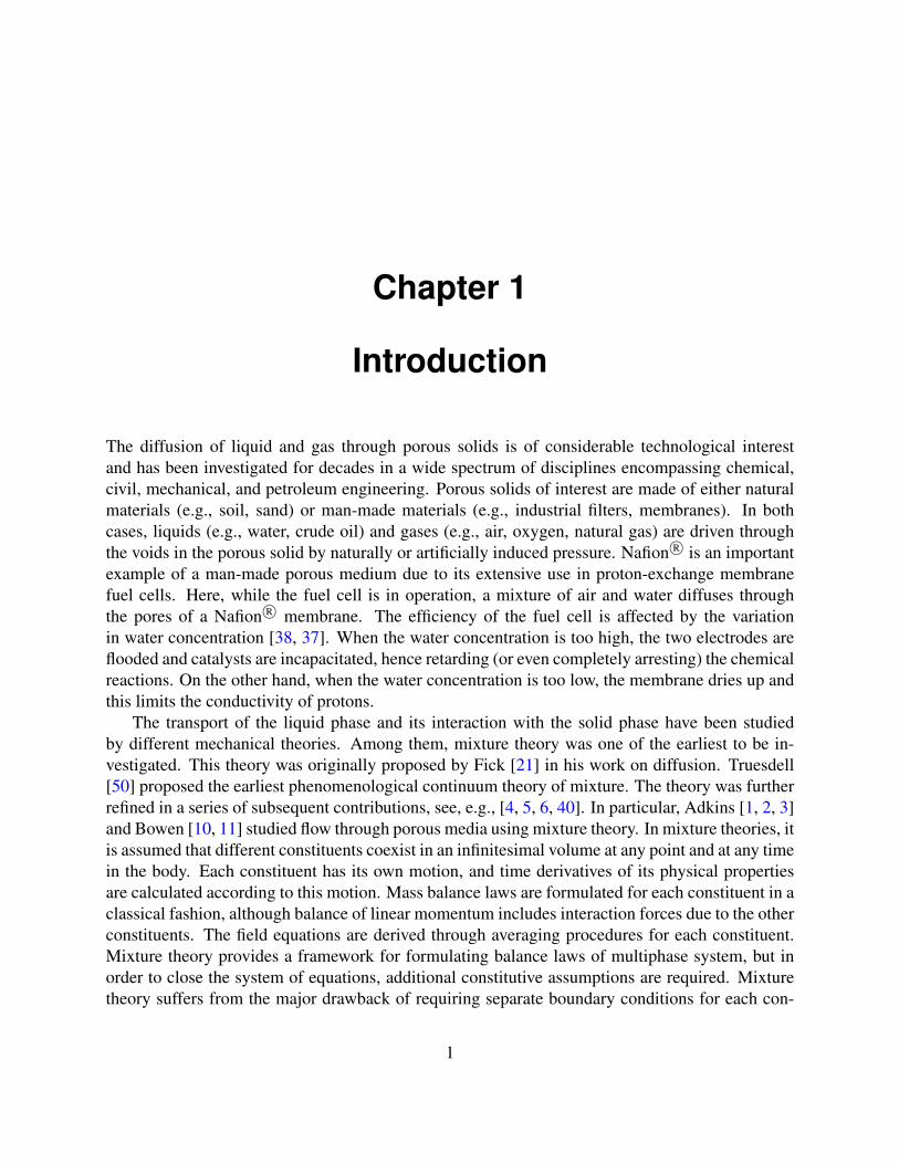
water concentration may cause substantial volumetric deformation (swelling) in Nafion R© mem-brane [20, 27], which may, in turn, compromise the integrity of the fuel cell. The swelling ofNafion R© has been measured and documented by Benziger [27]. Nafion R© membranes bulge al-most immediately as a water drop is placed on top of the membrane, and return to flatness as waterevaporates. A time sequence of the effect of a water drop on a Nafion R© membrane is shown inFigure 1.2.

In this thesis, a new continuum-based theory for the modeling of liquid flow through porousmedia is proposed and tested using the finite element method. The proposed theory draws fromearlier work, but includes several novelties that are specifically intended to broaden its applicability.Specifically, a key assumption here is that the dry solid and the voids are homogenized into asingle macroscopic solid medium. This makes sense for materials in which, regardless of theoverall porosity, the size of the pores is much smaller that the overall size of the medium. Inthis case, the liquid phase contributes additively to macroscopic balance laws without need forseparate balances for different phases. Moreover, since the balance laws are stated relative to the(homogenized) solid phase, the proposed theory relies on only one set of material time derivatives,namely those relative to the solid frame. Two different approaches will be explored within thisframework. First, single phase (liquid) diffusion is modeled, with liquid volume fraction chosenas a state variable and Fick’s law as the constitutive assumption. Then, multiphase (liquid and gas)diffusion is modeled, with liquid saturation as a state variable and Darcy’s law as the constitutiveassumption for diffusion in both phases. In the case of single phase diffusion, a linear relationshipbetween liquid volume fraction and its pressure is proposed as a constitutive assumption. Withthis assumption, Fick’s law coincides with Darcy’s law, since the gradient of liquid concentrationis proportional to the gradient of liquid pressure. By choosing liquid volume fraction or liquidsaturation as a state variable, both models permit the imposition of practical boundary conditionsand the precise identification of dry, partially saturated, and fully saturated conditions of the porousmedium, as well as the transitions from one such condition to another.

The organization of the thesis is as follows: Chapter 2 contains brief background of continuummechanics, as required for the presentation of the proposed models. Chapter 3 addresses singlephase fluid diffusion in an elastic porous solid, including weak forms of the balance laws requiredto formulate the finite element approximation. Chapter 4 extends the single phase continuum

4


model by including the gas phase and capillary pressure and by replacing Fick’s law with Darcy’slaw in the constitutive modeling. Chapter 5 documents representative numerical simulations ofthe single phase and the multiphase models, and further explores the role of gas in multiphasediffusion, as well as the constitutive assumption for capillary pressure. Concluding remarks areoffered in Chapter 6.

5

Chapter 2

Background

2.1 Continuum mechanics

2.1.1 Motion and deformation

Let the continuous solid body B occupy regionsR0 andR of volume vol(R0) and vol(R) at timest0 and t, respectively. These regions have oriented boundaries ∂R0 and ∂R, which are assumedsmooth enough to possess at every point unique outward unit normals N and n, respectively. Also,let X be the position vector of a point in R0 at time t0. The motion χ of the continuum maps Xto the vector x = χ(X, t) in R, as in Figure 2.1. The motion is assumed to be invertible for anygiven time t, and continuously differentiable in both of its arguments. The velocity of a materialpoint occupying x at time t is subsequently defined as

v(X, t) =∂χ(X, t)

∂t, (2.1)

where X is the position of the same material point at t0.Likewise, the deformation gradient at a point x inR relative to its image X inR0 is defined as

F(X, t) =∂χ(X, t)

∂X. (2.2)

An infinitesimal material volume element dV of the reference configuration (associated with theregion R0) is mapped to its image dv (associated with the region R) in the current configurationwith the motion χ, and it follows that

dv = det(F)dV . (2.3)

Since the motion is assumed invertible, J = det(F) 6= 0 for all (X, t), and without loss of gener-ality, it is further assumed that J > 0.

6

Chapter 2. Background

χ

X x

R

∂R

R0

∂R0

Figure 2.1: Motion of a continuum body

Scalar, vector and tensor functions can be expressed using the Lagrangian description, wherethe independent variables are the referential position X and time t, or expressed using the Euleriandescription, where the independent variables are the current position x and time t. For a scalarfunction ψ, the Lagrangian description can be written as

ψ = ψ(X, t) , (2.4)

and Eulerian description can be written as

ψ = ψ(x, t) = ψ(χ(X), t) = ψ(X, t) . (2.5)

The invertibility of the motion guarantees that the Lagrangian and Eulerian description of ψ areequivalent (i.e. each one can be derived from the other).

For a scalar function ψ with Lagrangian description ψ = ψ(X, t), the material time derivativeis defined as

ψ =∂ψ(X, t)

∂t. (2.6)

Based on the above definition, the material time derivative of ψ is the rate of change of ψ whilekeeping the referential position X fixed. For its Eulerian form ψ = ψ(x, t), the material timederivative is defined as

ψ =∂ ˜ψ(x, t)

∂t+ grad ψ · v , (2.7)

where the first term on the right hand side signifies the change with time of the function at thecurrent position x, and the second term is the convective part of the change of ψ.

7


2.1.2 Classic balance laws

2.1.2.1 Mass conservation

For any material part P of a body B, its mass should be conserved at any time t, i.e.,

d

dt

∫Pρdv = 0 . (2.8)

Using the Reynold’s transport theorem, the preceding equation can be written as∫P

(ρ+ ρ div v)dv = 0 . (2.9)

Provided that P is arbitrary, and upon invoking the localization theorem in (2.9), the local form ofthe mass conservation equation reads,

ρ+ ρ div v = 0 . (2.10)

2.1.2.2 Linear and angular momentum balance

The linear momentum of any infinitesimal volume element dv in a body can be defined as ρvdv.We admit the existence of two types of external forces acting on this element, namely body forceb and contact force t. The principle of linear momentum balance states that the rate of change oflinear momentum for any region P at time t equals the total external forces acting on this part, andcan be expressed as,

d

dt

∫Pρvdv =

∫Pρbdv +

∫∂P

tda . (2.11)

Taking into account the conservation of mass (2.10), the principle of linear momentum balancecan be expressed as ∫

Pρa dv =

∫Pρb dv +

∫∂P

t da . (2.12)

The Cauchy stress tensor T is defined such that t(x, t,n) = Tn. By substituting this expres-sion for t in (3.20) with T, and invoking the divergence theorem, linear momentum balance canbe written as ∫

Pρa dv =

∫Pρb dv +

∫P

div T dv . (2.13)

Local form of linear momentum balance can be readily expressed in the form

ρa = ρb + div T . (2.14)

The principle of angular momentum balance states that the rate of change of angular momen-

8


tum for any region P occupied at time t equals to the moment of all external forces acting on thispart, which is expressed as

d

dt

∫P

x× ρv dv =

∫P

x× ρb dv +

∫∂P

x× t(n) da . (2.15)

Same procedure can be applied to preceding equation, and after invoking linear momentumbalance, the above equation can be reduced to∫

Px,i × ti dv = 0 , (2.16)

and local form of angular momentum balance can be written as

x,i × ti = 0 . (2.17)

2.1.3 Invariance

A rigid-body motion is one in which all material particles in the body retain their distance to eachother. Now, take a motion χ of a body B such that x = χ(X, t), and another motion χ+ be definedfor B such that x+ = χ+(X, t), so that χ and χ+ differ only by a rigid body motion. Then, it canbe easily established that

x+ = Q(t)x + c(t) , (2.18)

where Q(t) is a time-varying proper orthogonal tensor (i.e. QQT = QTQ = I, det Q = 1,where I is the second-order identity tensor), and c(t) is a vector function of time, which signifies atranslation. The transformation of the velocity v under superposed rigid body motion is as follows

v+ =˙

Q(t)x + c(t) = Q(t)x + Q(t)v + c(t) . (2.19)

As shown with both the displacement and the velocity, transformation of kinematic terms isgoverned purely by geometry. However, transformation of kinetic terms and balance laws (bothmechanical and thermal) is governed by the principle of invariance under superposed rigid motion.This states that the balance laws should apply regardless of the choice of any superposed rigidmotion, hence they should be invariant under superposed rigid motions.

A tensor quantity is called objective if it transforms under superposed rigid body motions inthe same manner as its natural basis. A objective scalar ρ transform as

ρ+ = ρ . (2.20)

An objective referential vector V and spatial vector v transform according to

V+ = V , v+ = Qv . (2.21)

9


Second-order referential tensor A, spatial tensor B, and mixed tensor F = FiAei⊗EA are similarlyobjective if they transform as

A+ = A , B+ = QBQT , F+ = QF . (2.22)

2.2 Capillarity

Pa

Pw1

Pw2

Pa

h

Figure 2.2: Capillary pressure explained in a thin tube

Capillary action is the phenomenon in which liquid ascends through a thin tube or porousmedia, as shown in Figure 2.2. Capillarity occurs when the intermolecular cohesive force betweena liquid is substantially smaller than adhesive force between the liquid molecule and a medium’sinteracting surface. The difference between adhesive force and cohesive force creates surfacetension. The height to which liquid ascends inside a thin tube or porous media is determined bysurface tension and size of the tube or the pores.

Capillary pressures are generated where interfaces between two immiscible fluids exist in thepores. Equilibrium at the interface gives the basic relationship between the capillary pressure Pc,the interfacial tension σ, the contact angle θ and the pore radius a as

Pc =2σ cos θ

a. (2.23)

In practice, the interfacial tension and the contact angle are impossible to measure. Alterna-tively, the capillary pressure Pc is estimated by the height of liquid column rises in a thin tube, as

10


shown in Figure 2.2. Capillary pressure occurs at the top interface between air and water, and

Pc = Pw2 − Pa . (2.24)

At the surface of the water supply, the pressure of air and water are the same, i.e.

Pw1 = Pa . (2.25)

The pressure difference between Pw1 and Pw2 is determined by the height of water column in thetube,

Pw2 − Pw1 = ρgh . (2.26)

Combining (2.24),(2.25) and (2.26), the capillary pressure is now expressed as

Pc = ρgh . (2.27)

In Chapter 1, we briefly introduced Leverett’s experiment which is widely referenced to estab-lish constitutive relation between liquid saturation in porous materials and capillary pressure. Inhis experiment, a 6 m long vertical tube is filled with dry sand, and water is fed to the bottom ofthe tube with constant pressure. The top of sand is open to dry air. Water imbibition by capillarypressure through micro channels formed by sands, which is shown in Figure 2.3, takes weeks toreach a steady state.

Leverett measured the liquid concentration at each height in the sand, from which liquid satu-ration is calculated. Capillary pressure in sand is impossible to measure directly. However, the re-lationship between capillary pressure and height in micro channels is established in (2.27). Height,which is proportional to capillary pressure, is plotted against liquid saturation for several differenttypes of sand, all of which takes the general qualitative form shown in Figure 2.4. Leverett furtherproposed a dimensionless function, J-function, and expressed capillary pressure Pc in terms of theJ-function of liquid saturation φ and a constant σ which has dimension of pressure,

Pc = σJ(φ) . (2.28)

In this thesis, we will incorporate Leverett’s J-function (2.28) in our multiphase diffusionmodel, in which Darcy’s law is used as the governing equation for fluid diffusion through poroussolid materials. For a reliable estimate of the J-function, we will start from experiment measure-ments of capillary pressure and liquid saturation, and introduce a polynomial fit. In addition, wewill attempt to justify the form of the J-function by a simple physical argument involving diffusionof liquid through a solid containing an idealized set of microchannels.

11


Figure 2.3: Microchannels formed by sand inside the long tube

12


liquid saturation 10

J-functionofcapillary

pressure

Figure 2.4: Leverett J-function

13

Chapter 3

Single Phase of Liquid Diffusion in PorousSolid

This chapter concerns liquid diffusion through the voids of a porous solid. The voids and the solidjointly constitute a continuum macroscopic solid phase, which is endowed with a liquid volumefraction to model the liquid phase diffusion. Balance laws are postulated on the macroscopicsolid phase, and an initial/boundary-value problem is formulated, a finite element based solutionis proposed. Numerical simulations with the model are presented in the Chapter 5.

3.1 Concepts, definitions and constitutive relations

Consider a heterogeneous solid body B consisting of solid matter and voids (pores) of differentsizes and shapes. In this work, it is assumed that the characteristic size of the voids is much smallerthan the overall size of the body. Therefore, the material possesses a microstructure consisting ofsolid and void phases, as shown in Figure 3.1. This microstructure may be locally homogenized toyield a macroscopic continuous solid medium B. This medium will be endowed with momentumand density fields, as described below.

3.1.1 Porosity, liquid volume fraction and density

The porosity of a solid is generally defined as the ratio of the volume of voids over the total volumeof the porous solid. A local definition of porosity at the macroscale requires the introduction of arepresentative element of volume dv vol(R) which accurately resolves the microscopic poralstructure of the material. Therefore, the size of dv should be significantly larger than the averagesize of the pores. Now, the porosity φ of a solid at a macroscopic point may be defined as the ratioof the void volume to the volume dv of the porous solid in the representative element. It followsthat, under all circumstances, 0 ≤ φ < 1. It is assumed in this work that changes in the porosity φ

14

Chapter 3. Single Phase of Liquid Diffusion in Porous Solid

Solid Pore

B

Figure 3.1: Multiscale modeling and homogenization

due to the deformation of the solid are negligible.Some or all of the pores may be filled with a liquid, rendering the body partially or fully

saturated (otherwise, it is referred to as dry). In a partially saturated solid, a fraction of the voidsis occupied (either partially or fully) by the liquid, as in Figure 3.2. Specifically, assume that thevolume of the liquid in the representative element is dvl. Now, the liquid volume fraction φ isdefined locally in the macroscale by

dvl = φdv , (3.1)

where φ ≤ φ, with the strict equality holding for the fully saturated case.Mass conservation in the microscale implies that the macroscopic mass density ρ satisfies the

conditionρdv = ρldvl + ρsdv , (3.2)

where ρl and ρs are the densities of the pure liquid and the (dry) porous solid, respectively. Here,ρs is a homogenized density which accounts for the presence of voids in the solid.

Equations (3.1) and (3.2) now imply that

ρ = ρlφ+ ρs . (3.3)

15


solidvoidliquid

homogenization

liquiddry porous solid

macroscopic solid liquid saturation

Figure 3.2: Partially saturated porous medium

3.1.2 Liquid mass flux and linear momentum

Preliminary to the definition of liquid mass flux, let vl be the velocity of the liquid phase, which,in general, differs from the velocity of the macroscopic solid. Now, the flux of liquid mass throughthe solid can be expressed as

q = ρlφvr , (3.4)

where vr = vl − v is the relative velocity of liquid.Recalling the principal of invariance under superposed rigid motion, note first that both the

scalars ρl and φ are objective. To check objectivity of vr, let vl and v be the velocities of theliquid and the macroscopic solid at x. Under superposed rigid body motion, vl and v transformaccording to

v+l = Q(t)x + Q(t)vl + c(t) , v+ = Q(t)x + Q(t)v + c(t) , (3.5)

therefore vr transforms according to

vr+ = v+l − v+ = Q(t)vl −Q(t)v = Q(t)vr . (3.6)

Combining (3.4) and (3.6), it is easy to show that

q+ = ρ+φ+vr+ = Q(t)ρφvr = Q(t)q . (3.7)

16


which implies that the flux q is objective.Taking into account (3.3) and (3.4), the linear momentum ρsv + ρlφvl of the solid and liquid

phases may be written asρsv + ρlφvl = ρv + q . (3.8)

When the material is not fully-saturated, it is assumed that the flux of liquid mass obeys Fick’slaw [21]. Indeed, this stipulates that the flux of the liquid mass is proportional to the effectiveliquid density ρlφ and to the gradient of the liquid volume fraction, that is,

q = −Kρlφ gradφ , (3.9)

where K(> 0) is an isotropic diffusivity parameter.Equations (3.4) and (3.9) permit the representation of the liquid velocity vl as a function of the

velocity v of the macroscopic solid and the spatial gradient gradφ of the liquid volume fractionaccording to

vl = v −K gradφ . (3.10)

Therefore, if the densities ρs, ρl, the velocity v and the liquid volume fraction φ are adopted asstate variables in this theory, the preceding observation implies that the liquid velocity vl is not anindependent state variable. This is an important point of difference from classical mixture theory,as the latter requires the use of velocities for both the solid and the liquid phase.

3.1.3 Effective stress

The macroscopic solid and the liquid contribute to the stress in the body. Here, the cumulativeCauchy stress is assumed to take the form

T = Ts − pli , (3.11)

where Ts is the stress for the macroscopic solid, pl is the excess pressure due to the presence of theliquid phase, and i is the spatial second-order identity tensor. Similar additivity assumptions forstress have been previously utilized in [31, 23, 26]. Both T and Ts are assumed to be objective,therefore transform according to T+ = QTQT and T+

s = QTsQT .

In this work, the solid response is assumed hyperelastic. For specificity and given the moderatemagnitude of the deformation, the solid is taken to obey the Kirchhoff-Saint Venant constitutivelaw, according to which the second Piola-Kirchhoff stress Ss = JF−1TsF

−T is given by

Ss = λ tr(E)I + 2µE . (3.12)

Here, E is the Lagrangian strain, while λ, µ are elastic constants for the macroscopic solid.The excess pressure due to the liquid phase should clearly depend on the liquid volume fraction,

17


that is pl = pl(φ). For simplicity, a linear relation is assumed here in the form

pl = Cφ , (3.13)

where C is a material constant (see [23] for a related assumption).

3.2 Balance laws

Consider a part of the macroscopic solid, which occupies an arbitrary closed and bounded regionP ⊂ R with smooth boundary ∂P at time t.

Balance of mass and linear momentum are formulated below by examining the material inregion P . Here, all material time derivatives of integrals over P are defined by keeping materialparticles of the macroscopic solid fixed.

3.2.1 Balance of mass

The rate of change of total mass for the region P occupied by the macroscopic solid at time t takesthe form

d

dt

∫Pρ dv =

d

dt

∫Pρs dv +

d

dt

∫Pρlφ dv , (3.14)

where use is made of (3.3). Since the mass of the macroscopic solid material is conserved, thepreceding equation readily reduces to

d

dt

∫Pρ dv =

d

dt

∫Pρlφ dv . (3.15)

This is contrasted to the conventional mass balance statement in (2.8). Also, since all changes ofthe liquid mass in P are due to the flux of the liquid q at the boundary ∂P , it follows from (3.15)that the balance of total mass may be expressed simply as

d

dt

∫Pρlφ dv = −

∫∂P

q · n da . (3.16)

Appealing to the Reynolds’ transport, divergence and localization theorems, the integral state-ment (3.16) gives rise to a corresponding local statement, which is given by

d

dt(ρlφ) + ρlφ div v = − div q . (3.17)

Alternatively, combining (3.15) and (3.16), mass balance may be expressed in term of the macro-

18


scopic mass density asρ+ ρ div v = − div q . (3.18)

Again, the local form of mass balance is contrasted to the conventional form (2.10) to appreciatethe effect of the liquid flux q. Also, in comparing equation (3.18) to the corresponding massbalance equation in classical mixture theory, it is noted that the latter is obtained by summingthe respective balance equations for the different phases and defining an equivalent material timederivative as a linear combination of the density-weighted derivatives of the individual phases.Clearly, no such summation is needed here, because the mass balance equation is written withrespect to the macroscopic solid and, hence, incorporates changes to the fluid mass through theflux term q.

The conventional local form of mass balance is recovered from (3.18) by merely setting q = 0.

3.2.2 Balance of linear momentum

Balance of linear momentum necessitates that the rate of change of total linear momentum for theregion P occupied by the macroscopic solid at time t be equal to the external forces acting on thematerial and the flux of linear momentum−(ρlφvl)v

r ·n through the boundary ∂P . This translatesto

d

dt

∫P

(ρsv + ρlφvl) dv =

∫Pρb dv +

∫∂P

t da−∫∂P

(ρlφvl)vr · n da , (3.19)

where t = Tn is the traction vector on ∂P . Recalling (3.4) and (3.8), the preceding equation maybe equivalently rewritten as

d

dt

∫P

(ρv + q) dv =

∫Pρb dv +

∫∂P

t da−∫∂P

(q · n)vl da . (3.20)

Invoking, again, the Reynolds’ transport theorem and also the mass balance equation (3.18)and the divergence theorem, the integral statement of linear momentum (3.20) may be recast in theform∫

P

(ρdv

dt− v div q +

dq

dt+ q div v

)dv =

∫Pρb dv +

∫P

div T dv −∫P

div (vl ⊗ q) dv .

(3.21)

The corresponding local form follows readily from (3.21), and reads

ρdv

dt− v div q +

dq

dt+ q div v = ρb + div T− div (vl ⊗ q) . (3.22)

Again, setting q = 0 reduces (3.22) to the conventional local form of linear momentum bal-ance.

19


3.3 Finite element implementation

3.3.1 Weak forms

In this section, weak counterparts of the local balance equations (3.17) and (3.22) are constructedpreliminary to finite element discretization.

For mass balance, equation (3.17) is first weighted by a scalar test function η, then integratedover P , so that, upon invoking integration by parts and the divergence theorem, it leads to∫

Pηρl

dφ

dtdv +

∫Pηρlφ div v dv −

∫P

grad η · qdv +

∫∂Pηq · n da = 0 . (3.23)

Likewise, for balance of linear momentum, equation (3.22) is contracted with an arbitraryvector test function ξ and integrated over the domain P . This leads to∫

Pξ · ρdv

dtdv −

∫Pξ · v div q dv +

∫Pξ · dq

dtdv +

∫Pξ · q div v dv −

∫Pξ · ρb dv

−∫Pξ · div T dv +

∫Pξ · vl div q dv +

∫Pξ ·[(grad vl)q

]dv = 0 . (3.24)

Applying integration by parts and the divergence theorem to the second and sixth terms on theleft-hand side of (3.24), one may recast the preceding weak form as∫

Pξ · ρdv

dtdv +

∫P

[(grad ξ)q

]· v dv +

∫Pξ ·[(grad v)q

]dv −

∫∂P

[(ξ · v)q

]· n da

+

∫Pξ · dq

dtdv +


∫Pξ · ρb dv +

∫P

grad ξ ·Tdv −∫∂P

ξ · t da

+

∫Pξ · vl div q dv +


]dv = 0 . (3.25)

The last two terms on the left-hand side of (3.25) may be further rewritten with the aid of integrationby parts and the divergence theorem as∫Pξ ·vl div q dv+


]dv =

∫∂P

[(ξ ·vl)q

]·n da−

∫P

[(grad ξ)q

]·vl dv . (3.26)

20


This leads to an alternative expression for the weak form of linear momentum balance as∫Pξ · ρdv

dtdv +

∫P

[(grad ξ)q

]· (K gradφ) dv +

∫Pξ ·[(grad v)q

]dv

+

∫Pξ · dq

dtdv +


∫Pξ · ρb dv +

∫P

grad ξ ·T dv

−∫∂P

ξ · t da−∫∂P

[(ξ · (K gradφ)

)q]· n da = 0 , (3.27)

where the liquid velocity is eliminated by using (3.10).

3.3.2 Space and time discretization

In the finite element setting, the domain of the continuum macroscopic porous solid body is ap-

proximated by a set Ω of nonoverlapping elements such that R ≈ Ω =

nelmt⋃I=1

ΩI , where nelmt is

number of elements. The macroscopic solid displacement u and liquid volume fraction φ, as wellas test functions ξ and η are approximated by nodal interpolations as

u(x, t) =

Nnode∑I=1

NI(x)uI(t) , φ(x, t) =

Nnode∑I=1

NI(x)φI(t)

ξ(x, t) =

Nnode∑J=1

NJ(x)ξJ(t) , η(x, t) =

Nnode∑J=1

NJ(x)ηJ(t) . (3.28)

Here, nnode is the number of nodes in an element, NI(x) is the shape function at node I , uI(t),φI(t), are the nodal values of the solid displacement and liquid volume fraction at node I and timet, and ξI(t), ηI(t) are corresponding nodal values of test function ξ and η at node I and time t.

Substitute the spatial interpolation (3.28) in mass balance equation (3.23), The indicial form ofits residual at I node becomes

ηI[∫PNIρlφ dv +

∫PNIρlφ div v dv −

∫PNI,mqmdv +

∫∂PNIqmnm da

]= 0 . (3.29)

The arbitrariness of the testing function β implies that the residual force RI vanishes, that is

RI =

∫PNIρlφ dv +

∫PNIρlφ div v dv −

∫PNI,mqmdv +

∫∂PNIqmnm da = 0 . (3.30)

Same procedure is applied to linear momentum (3.27), the indicial form of its residual at the

21


I th node becomes

ξIi[∫PNIρajδij dv +

∫PNI,mqnKφ,jδmnδij dv +

∫PNIvj,mqnδijδmn dv

+

∫PNI

dqjdtδij dv +

∫PNIqjδij div v dv −

∫PNIρbjδij dv +

∫PNI,mTjmδijδmn dv

−∫∂PNItjδij da−

∫∂PKNIφ,jqnnmδijδmn da

]= 0 , (3.31)

where i, j, m, n are spatial coordinate indices.Again, the arbitrariness of the testing function ξ implies that the residual force RIi vanishes,

that is

RIi =

∫PNIρajδij dv +

∫PNI,mqnKφ,jδmnδij dv +

∫PNIvj,mqnδijδmn dv

+

∫PNI

dqjdtδij dv +

∫PNIqjδij div v dv −

∫PNIρbjδij dv +

∫PNI,mTjmδijδmn dv

−∫∂PNItjδij da−

∫∂PKNIφ,jqnnmδijδmn da = 0 . (3.32)

The final assembled residual equation can be written as a nonlinear function of the displace-ment u, the velocity v, the acceleration a, the liquid volume fraction φ, and the time derivative ofliquid volume fraction φ, as

R(u,v, a, φ, φ) = 0 . (3.33)

To solve the coupled system of first- and second-order ordinary differential equations in time, aone-step time integration algorithm is introduced. In a typical time interval (tn, tn+1] by using animplicit Newmark scheme [36], such that

un+1 = un + vn∆tn +1

2[(1− 2β)an + 2βan+1] ∆t2n

vn+1 = vn + [(1− γ)an + γan+1] ∆tn

φn+1 = φn +[(1− γ)φn + γφn+1

]∆tn ,

(3.34)

where (·)n = (·) |n= (·)(tn), ∆tn = tn+1 − tn, and β ∈ (0, 1/2], γ ∈ (0, 1] are the Newmarkparameters. The typical choice for the latter is β = 1/4, γ = 1/2, which compares to the classicaltrapezoidal rule.

A Newton-Raphson method is adopted to solve the nonlinear algebraic equation Ri = 0 re-

22


sulting from the application of (3.34) to (3.33). This can be written in component form as

R(k+1)i = R

(k)i +

∂Ri

∂αj

∣∣∣(k)

dα(k)j = 0 , (3.35)

where αj is one of the variables at time tn+1, and k is the iteration number for the Newton-Raphsonmethod. Stiffness matrix for solving equation (3.33) is defined as

K(k)ij = −∂Ri

∂αj

∣∣∣(k)

(3.36)

Since the residual function R can be expressed with the aid of (3.34) only in terms of u and φ,the stiffness matrix is written as

Kij∆uj = −∂Ri

∂uj∆uj −

∂Ri

∂vk

∂vk∂uj

∆uj −∂Ri

∂ak

∂ak∂uj

∆uj , (3.37)

and

Kij∆φj = −∂Ri

∂φj∆φj −

∂Ri

∂φk

∂φk∂φj

∆φj , (3.38)

where ∆uj , ∆φj are increments of the unknown variables.Newmark formulas (3.34) give

∂vk∂uj

=γ

β∆tδkj ,

∂ak∂uj

=1

β∆t2δkj , (3.39)

and∂φk∂φj

=1

γ∆tδkj . (3.40)

Stiffness matrix K can be readily calculated as following,

Kij∆uj = −∂Ri

∂uj∆uj −

γ

β∆t

∂Ri

∂vk∆uj −

1

β∆t2∂Ri

∂ak∆uj , (3.41)

andKij∆φj = −∂Ri

∂φj∆φj −

1

γ∆t

∂Ri

∂φk∆φj . (3.42)

The detailed consistent linearization of the residual R weak forms with respect to u and φ isderived in the Appendix A.

23

Chapter 4

Multiphase Diffusion in Porous Solid

This chapter expands the modeling capability to include multiphase flow. With the same continuummacroscopic solid phase, porosity is again viewed as a local material property. To model liquiddiffusion in the presence of a gas phase, capillary pressure is included in the expanded model.After forming the balance laws on the macroscopic solid, and setting the initial/boundary-valueproblem, a finite element solution is again developed, and numerical simulations are discussed inChapter 5.

4.1 Definitions

4.1.1 General definitions

Consider a porous body B consisting of solid matter and voids of different sizes and shapes. Whenthe body is dry, all the pores are occupied by gas (typically, air). Otherwise, the pores may beeither partially or fully occupied by liquid matter, as shown in Figure 4.1.

Next, assume, again, that the characteristic size of the voids be much smaller than the overallsize of the body. Now, the porous solid can be locally homogenized to yield a macroscopic con-tinuous solid endowed with a density field ρs. This homogenization altogether excludes the liquidand gas phases.

The bulk porosity ε (0 ≤ ε ≤ 1) may now be defined at any point of the macroscopic solid asthe ratio of the volume of voids to the volume of the macroscopic solid in a representative elementV centered at the point. Such a definition is meaningful provided that the porosity field is well-defined for a representative element volume which is much smaller than the total volume of thebody, that is, if vol(V) vol(R).

The preceding homogenization procedure may be employed to also define the saturation φ ata point as the ratio of the volume of liquid to the volume of the void in the representative elementvolume. Therefore, φ = 0 corresponds to dry pores and φ = 1 to fully saturated ones. In thepartially saturated case (0 < φ < 1), gas occupies any portion on the pores that is not filled with

24

Chapter 4. Multiphase Diffusion in Porous Solid

Liquid Soild Void liquid air

Figure 4.1: Partially saturated porous solid

liquid. Therefore, the total density ρ of the porous medium is

ρ = ρs + ρlεφ+ ρgε(1− φ) , (4.1)

where ρl and ρg are densities of the liquid and gas phases. Both densities are taken to be constant:for the liquid, this is an immediate implication of homogeneity and incompressibility, while forthe gas it is due to the assumption that the gas is allowed to move freely through the pores withoutbeing subject to compression.

The diffusion of liquid and gas matter in the porous medium is characterized by the fluxes ofliquid ql and gas qg in the macroscopic solid, defined as

ql = ρlεφvrl , qg = ρgε(1− φ)vrg . (4.2)

Here, vrl and vrg are the liquid and gas velocities relative to the macroscopic solid. These are relatedto the respective absolute velocities vl and vg as vrl = vl − v and vrg = vg − v. Repeating againthe argument in Section 3.1.2, it is easy to conclude that the two fluxes are objective.

4.2 Balance laws

Consider a part of the macroscopic solid, which occupies an arbitrary closed and bounded regionP ⊂ R with smooth boundary ∂P having outward normal n at time t.

Balance of mass and linear momentum are formulated below by examining the material inregion P . Here, all material time derivatives of integrals over P are defined by keeping material

25


particles of the macroscopic solid fixed.

4.2.1 Balances of mass

Since all balance laws are formulated on a material domain P relative to the macroscopic solidmaterial, mass conservation for the macroscopic solid is automatically satisfied. Additional massbalance laws are required for the liquid and gas phases.

For the liquid phase, the rate of change of mass equals the flux of liquid leaving the domainfrom the boundary ∂P , hence it takes the form

d

dt

∫Pρlεφ dv = −

∫∂P

ql · n da . (4.3)

Upon using the Reynolds’ transport theorem and the divergence theorem, the local form of (4.3) isderived as

d(ρlεφ)

dt+ ρlεφ div v = − div ql . (4.4)

Likewise, the mass balance for the gas phase is written in integral form as

d

dt

∫Pρgε(1− φ) dv = −

∫∂P

qg · n da , (4.5)

with its local counterpart expressed as

d(ρgε(1− φ)

)dt

+ ρgε(1− φ) div v = − div qg . (4.6)

4.2.2 Balance of linear momentum

The proposed theory relies on a single linear momentum balance law, rather than on individualbalances for each phase. This circumvents the need to resolve all force interactions between theconstituent phases.

The rate of change of the total linear momentum is equal to the total external force acting onthe material and the flux of linear momentum of the liquid and gas phases. This means that theintegral statement of linear momentum balance for the domain P is given as

d

dt

∫P

(ρsv + ρlεφvl + ρgε(1− φ)vg) dv =∫Pρb dv +

∫∂P

t da−∫∂P

(ql · n)vl da−∫∂P

(qg · n)vg da . (4.7)

26


Taking into account (4.1) and (4.2), the left-hand side of (4.7) may be rewritten as

d

dt

∫P

(ρsv + ρlεφvl + ρgε(1− φ)vg

)dv =

d

dt

∫P

(ρv + ql + qg) dv . (4.8)

Using the mass balance equations (4.4) and (4.6) and the Reynolds’ transport theorem, theright-hand side of the above equation becomes

d

dt

∫P

(ρv + ql + qg) dv =∫P

(ρdv

dt− v(div qg + div ql) +

dqgdt

+ qg div v +dqldt

+ ql div v)dv . (4.9)

Combining (4.9) and (4.7) and invoking the divergence theorem, the local form of the linearmomentum balance equation is deduced in the form

ρdv

dt− v(div qg + div ql) +

dqgdt

+ qg div v +dqldt

+ ql div v =

ρb + div T− div qgvg − (grad vg)qg − div qlvl − (grad vl)ql , (4.10)

where T is the Cauchy stress of the body.

4.3 Constitutive assumptions

The balance laws furnish a total of five equations, two from mass and three from linear momentumbalance to determine twelve unknowns, that is the macroscopic solid displacement u, the liquidsaturation φ, the liquid pressure pl, the gas pressure pg, the relative liquid velocity vrl and therelative gas velocity vrg. Therefore, closure of the system necessitates the introduction of sevenconstitutive equations.

The diffusion of liquid and gas matter in the macroscopic solid is assumed to be governedby Darcy’s law, which states that diffusion is driven by (and is proportional to) the gradient ofpressure. Therefore, the constitutive assumptions for the relative velocities of liquid and gas takethe form

vrl = −klµl

gradPl , vrg = −kgµg

gradPg , (4.11)

where kl, kg, µl, and µg are liquid and gas permeabilities and viscosities, respectively.The final equation needed to close the system concerns the capillary pressure, which is the

difference in pressure across the interface between gas and liquid in equilibrium, that is

Pc = Pl − Pg . (4.12)

27


Leverett [33] introduced a dimensionless function J(φ) to which the capillary pressure Pc is as-sumed to be proportional, that is

Pc = σJ(φ) , (4.13)

where σ is a constant that has the dimension of pressure. Several analytical expressions of theLeverett J-function have been proposed in the literature for different applications, see, e.g., [12,25, 51].

Here, we offer a qualitative argument for the overall form of the J-function. One may considerporous media as comprising many microchannels formed by pores. Liquid may diffuse throughsuch microchannels as in the idealized porous medium whose cross-section is locally characterizedby the regular structure of the representative area element depicted in Figure 4.2. Denoting the

(a) Dry (b) Low saturation

(c) High saturation (d) Full saturation

Figure 4.2: Local structure of the representative area element of an idealized porous medium atfour different states of saturation (“wet” microchannels are shown as filled blue circles and “dry”ones are shown as unfilled circle)

(average) capillary pressure in a non-saturated microchannels pc and letting the (average) cross-section of a microchannel be A, the local homogenized capillary pressure Pc is

Pc =NpcA

A, (4.14)

whereN is total number of non-saturated microchannels andA is the total area of the representative

28


area element of the cross-section. When the porous medium is essentially dry as in Figure 4.2a,(that is, φ approaches zero), all the microchannels are non-saturated, therefore N is large, whichyields a high capillary pressure Pc. As the medium gets progressively more saturated with liquid(hence, φ increases), as in Figure 4.2b,c, N decreases, and so does the capillary pressure Pc. In thelimiting case of full saturation (φ = 1) depicted in Figure 4.2d, N approaches zero, as does Pc.In conclusion, the preceding argument implies that the J-function is monotonically decreasing tozero with increasing values of φ. While the argument suggests linearity of J in N , this does notnecessarily translate to linearity of J in φ, since the geometric structure of the microchannels is farmore complex than that of straight parallel tubes assumed here.

Here, we further explore the nonlinearity of the J-function first by relating area saturation andthe volume saturation. By definition, area saturation φarea is the ratio of the area of saturatedmicrochannels to the total area, so NA

Ain (4.14) is equal to 1− φarea, and this equation implies

Pc ∝ 1− φarea . (4.15)

It is reasonable to assume that microchannels in different orientations are saturated at the samepace, so volume saturation φ and area saturation φarea follow a simple relation as below

φ = φ32area . (4.16)

The two preceding equations give us a nonlinear relation between the J-function and φ, which isplotted in Figure 4.3.

Next, we consider nonlinearity of the J-function caused by the statistical distribution of theareas of microchannels. Let the areas of the microchannels follow a random distribution, and re-call that capillary pressure of each microchannel is a function of the radius of the microchannel,as given in (2.23). Also, let the microchannel with higher capillary pressure be saturated beforethe ones with lower capillary pressure. For the cases where the areas of the microchannels followa normal distribution or a uniform distribution, the J-function takes nonlinear forms as illustratedagain in Figure 4.3. Therefore, in summary, the capillary pressure decreases as the porous mediumis saturated progressively, and the J-function takes a nonlinear form which is caused by the geom-etry of the microchannels in the porous medium and the randomness in the pore sizes.

In this thesis, we assume that the J-function depends polynomially on φ where all polynomialcoefficients have the dimension of pressure and are obtained by curve-fitting of experimental mea-surements of the capillary pressure for different values of liquid saturation. In particular, a simplecubic polynomial approximation is considered in the form

Pc = c1φ3 + c2φ

2 + c3φ+ c4 , (4.17)

where the coefficients ci, i = 1 − 4, are determined for each porous medium from experimentaldata [39, 8, 19]. It will be shown in Section 5.2 that this approximation captures with accuracy the

29


0 1

saturation φ

capi

llary

pres

sure

volume saturationnormal distribution

uniform distribution

Figure 4.3: Nonlinear J-function explained by saturation and random distribution of areas of themicrochannels

salient features of the dependency of Pc on φ for different types of porous media.The macroscopic solid, gas and liquid phases contribute to the homogenized stress in the body,

and the cumulative Cauchy stress is assumed to be in the form

T = Ts − (Pl + Pg)i (4.18)

where Ts is the stress for the macroscopic solid, and i is spatial second-order identity tensor.A special case of the theory arises when the capillary pressure is assumed to be linear in φ,

according toPc = σ(1− φ) . (4.19)

It follows, upon recalling (4.2), (4.11), and (4.12), that the liquid mass flux is reduced to

ql = −ρlεφklµl

(gradPg − σ gradφ) . (4.20)

In addition, if the gas pressure is taken to be uniform inside the porous medium, the equation for

30


liquid flux is further reduced to be

ql = Kdρlεφ gradφ , (4.21)

where liquid diffusivity constantKd is given by klσµl

. This equation now coincides to the one derivedin an earlier work [54]. Also, gas mass flux is zero through out the porous medium in this case dueto uniform gas pressure, therefore mass balance for gas is automatically satisfied.

4.4 Finite element approximation

4.4.1 Weak forms

In this section, weak forms of the local balance equations (4.4), (4.6) and (4.10) are constructed byway of background to the finite element approximation. element time and space discretization.

For liquid and gas mass balance, equations (4.4) and (4.6) are first weighted by arbitrary scalartest functions η and ζ , then integrated over P . After using integration by parts and invoking thedivergence theorem, the weak forms of liquid and gas mass balance become∫

Pηρlε

dφ

dtdv +

∫Pηρlεφ div v dv −

∫P

grad η · ql dv +

∫∂Pηql · n da = 0 (4.22)

and∫Pζρgε

d(1− φ)

dtdv+

∫Pζρgε(1−φ) div v dv−

∫P

grad ζ ·qg dv+

∫∂Pζqg ·n da = 0 , (4.23)

respectively.Likewise for linear momentum balance, equation (4.10) is first weighted by an arbitrary vector

test function ξ, and integrated over P . Again, after the straightforward application of integrationby parts and the divergence theorem, the weak form of linear momentum balance is expressed as∫

Pξ · ρdv

dtdv −

∫∂P

[(ξ · v)qg

]· n da+

∫P

[(grad ξ)qg

]· v dv +

∫Pξ ·[(grad v)qg

]dv

+

∫Pξ·dqgdt

dv+

∫Pξ·qg div v dv−

∫∂P

[(ξ · v)ql]·n da+

∫P

[(grad ξ)ql

]·v dv+

∫Pξ·[(grad v)ql

]dv

+

∫Pξ·dqldt

dv+

∫Pξ·ql div v dv−

∫Pξ·ρb dv+

∫P

grad ξ·T dv−∫∂P

ξ·t da+

∫∂P

[(ξ·vg)qg

]·n da

−∫P

[(grad ξ)qg] · vg dv +

∫∂P

[(ξ · vl)ql

]· n da−

∫P

[(grad ξ)ql

]· vl dv = 0 . (4.24)

The preceding equation may be simplified by combining the second and third term with the fif-

31


teenth and sixteenth term, and also the seventh and eighth with the seventeenth and eighteenthterm, leading to∫

Pξ · ρdv

dtdv +

∫∂P

[(ξ · vrg)qg

]· n da−

∫P

[(grad ξ)qg

]· vrg dv +

∫Pξ · [(grad v)qg] dv

+

∫Pξ · dqg

dtdv +

∫Pξ · qg div v dv +

∫∂P

[(ξ · vrl )ql

]· n da−

∫P

[(grad ξ)ql

]· vrl dv

+

∫Pξ·[(grad v)ql

]dv+

∫Pξ·dqldt

dv+

∫Pξ·ql div v dv−

∫Pξ·ρb dv+

∫P

grad ξ·T dv−∫∂P

ξ·t da = 0 .

(4.25)

4.4.2 Space and time discretization

A finite element approximation is effected on the weak forms (4.22), (4.23) and (4.25). Owing tothe arbitrariness of the test functions η, ζ and ξ, the weak forms give rise to a coupled system ofintegro-differential equations with the macroscopic solid displacement u, liquid saturation φ andgas pressure pg as unknown variables.

Following standard procedure, semi-discretization is employed for the solution of (4.22), (4.23)and (4.25) with displacement-like finite element approximation used for the spatial discretizationof u, φ and Pg, similar to the procedure showed in Section 3.3.2. This results in a coupled system offirst- and second-order ordinary partial differential equations in time. These, in turn, are integratedin a typical time interval (tn, tn+1] using an implicit Newmark method [36], according to which

un+1 = un + vn∆tn +1

2[(1− 2β)an + 2βan+1] ∆t2n ,

vn+1 = vn + [(1− γ)an + γan+1] ∆tn ,

φn+1 = φn +[(1− γ)φn + γφn+1

]∆tn ,

Pg,n+1 = Pg,n +[(1− γ)Pgn + γPgn+1

]∆tn .

(4.26)

The resulting nonlinear algebraic equations are solved at any discrete time tn+1 with the Newton-Raphson method. This requires consistent linearization of the weak forms with respect to u, φ andPg, which is derived in the Appendix.

32

Chapter 5

Numerical Simulations

5.1 Single Phase Liquid Diffusion in Porous Solid

The finite element formulation of the model described in Chapter 3. was implemented in thegeneral-purpose nonlinear program FEAP, which is partially documented in [49, 48]. The modeland its numerical implementation were tested on three representative simulations discussed below.All simulations employed 8-node isoparametric brick elements with full 2×2×2 Gaussian quadra-ture. In addition, the time integration parameters defined in Section 3.3.2 were set to β = 0.25and γ = 0.5.

The material properties in the simulations were chosen for Nafion R©, which is suitable formodeling within the proposed theory, owing to the small size of its pores (with diameter of 20–30 nm [22]) compared to the typical thickness of industrial Nafion R© membranes (0.175 mm [34]).The Nafion R© properties were set to: (λ, µ) = (0.40×107, 0.27×107) Pa [43], ρs = 2×103 kgr/m3

[43], ρl = 103 kgr/m3, φ = 0.4 [47], K = 1.0 × 10−10 m2/s [35], and C = 106 Pa. The lastparameter was chosen heuristically such that the liquid excess pressure pl in (3.13) be in the rangeof one atmosphere at saturation.

5.1.1 Stretching of a saturated cube

A 0.5 mm cube made of saturated Nafion R© is stretched uniformly using displacement control onone face while being fixed on the opposite face and free on all four lateral faces. Zero liquid fluxboundary conditions are enforced on the whole boundary. The imposed stretching is applied attime t = 0 and the body is subsequently allowed to reach steady-state.

A uniform 10 × 5 × 5 mesh is used to discretize the domain, with the finer resolution alignedwith the direction of stretching (here, the x-direction). Also, time integration is performed withconstant step-size ∆t = 10−6 s.

Figure 5.1 shows the distribution of the liquid volume fraction along the centerline of the cubein the x-direction at three different times and for stretch λ = 0.1. At t = 10−6 s, the body is

33

Chapter 5. Numerical Simulations

0.33

0.34

0.35

0.36

0.37

0.38

0.39

0.4

0.41

1 2 3 4 5 6 7 8 9 10 11

nodal index in x direction

liqui

dvo

lum

efr

actio

nt=10−6 st=10−5 st=10−4 s

Figure 5.1: Stretching of a saturated cube: Liquid volume fraction at the nodes along the centerlineof the stretch direction at different times (nodes are indexed from 1 to 11 with the latter being onthe stretched side)

essentially saturated away from the stretched end, while near this end its liquid volume fractionexhibits a precipitous drop. At t = 10−5 s, the distribution of the liquid volume fraction is muchsmoother reflecting the flow of liquid toward the stretched end of the body, while at t = 10−4 sthe volume fraction is spatially uniform and below the saturation limit due to the attainment ofsteady-state.

Next, the cube is stretched in increments of ∆λ = 0.1 up to a total stretch of λ = 0.4. Aftereach stretch increment, the body is allowed to reach steady-state before the next increment is im-posed. The relation between the liquid volume fraction at steady-state and the stretch is illustratedin Figure 5.2 and shows the expected monotonic decrease. The same figure also depicts the totalvolume of the liquid, which remains constant throughout the stretch loading owing to the zero-fluxboundary conditions.

34


0.2

0.25

0.3

0.35

0.4

1 1.1 1.2 1.3 1.4 1.5

stretch λ

liqui

dvo

lum

efr

actio

n

2.8

3

3.2

1 1.1 1.2 1.3 1.4 1.5

stretch λ

liqui

dvo

lum

e(×

10−

11)×10−11

Figure 5.2: Stretching of a saturated cube: Liquid volume fraction at steady-state as a function ofstretch (top) and conservation of liquid volume (bottom)

5.1.2 Squeezing of a saturated cube

A 0.5 mm cube of saturated Nafion R© is compressed uniformly on one of its faces using displace-ment control, while the opposite face remains fixed and each of the four lateral faces is free to slideon its own plane only. The liquid may escape from the compressed face, while all other faces areassumed to be impermeable. The block is initially squeezed to λs = 93% while keeping the liquidvolume fraction to the saturation value of φ = 0.4 on the compressed face. Then, it is stretchedback to its original shape, where it is kept until the liquid volume fraction reaches steady state.During the stretching and until steady state is attained, the compressed face is subject to zero liq-uid flux conditions. Each of the three loading stages is imposed proportionally over a period of0.1 s.

A uniform 5×5×5 mesh is used in this problem and the time step-size is set to ∆t = 1 ms. Asillustrated in Figure 5.3, the total volume of the liquid decreases during squeezing, then remainsconstant while the body returns to its original configuration. At the same time, the total volume of

35


the porous medium initially decreases and then increases back to its original value.

4.6

4.8

5

50 100 150 200 250 3000.36

0.38

0.4

time (ms)

volu

me

ofliq

uid

(m3) ×10−11

liqui

dvo

lum

efr

actio

n

1.15

1.17

1.19

1.21

1.23

1.25

50 100 150 200 250 300

time (ms)

tota

lvol

ume

(m3)

×10−11

×10−10

liquid volumeliquid volume fraction

Figure 5.3: Squeezing of a saturated cube: Liquid and total volume as a function of time

The same block is subsequently subjected to repeated squeezing and stretching of the samemagnitude and rate as before. In this case, liquid escapes from the solid block repeatedly until thesolid material pushes enough of it out of the block to reach a steady state of liquid volume fraction.To prevent back-flow into the block, the fixed liquid volume fraction boundary condition on thecompressed face during squeezing is chosen to be equal to the minimum of the current steady-stateliquid volume fraction and the asymptotic liquid volume fraction φa at maximum squeezing. Thelatter is equal, in this case, to

φa =λsV − (1− φ)V

λsV=

0.93− (1− 0.4)

0.93.= 0.35 , (5.1)

where V denotes the initial volume of the block. The preceding definition is predicated upon theassumption that the solid matter (being hyperelastic) returns to its original volume when the liquidvolume reaches a steady value after a sufficient number of squeezes. The results of this numerical

36


simulation are illustrated in Figure 5.4, where it is specifically shown that this steady volume ofliquid is reached after only three successive squeezes.

4

4.2

4.4

4.6

4.8

5

0 200 400 600 800 1000 12000.3

0.32

0.34

0.36

0.38

0.4

time (ms)

volu

me

ofliq

uid

(m3) ×10−11

liqui

dvo

lum

efr

actio

n

1.15

1.17

1.19

1.21

1.23

1.25

0 200 400 600 800 1000 1200

time (ms)

tota

lvol

ume

(m3)

×10−11

×10−10

liquid volumeliquid volume fraction

Figure 5.4: Squeezing of a saturated cube: Liquid and total volume as a function of time for thecase of repeated squeezing

5.1.3 Flexure of a Nafion R© film due to water absorption

It has been experimentally observed that when placing a water droplet on a dry thin film made ofNafion R©, the region surrounding the droplet initially exhibits a bulge, which later disappears as thewater evaporates and/or is diffused into the film [27]. To simulate this experiment, a water dropletis idealized by means of a prescribed liquid volume fraction boundary condition on a square regionwith 3 mm side at the center of the top surface of a 10× 10× 0.125 mm Nafion R© block. The latteris fixed on all of its four lateral faces and zero liquid flux boundary condition is imposed on allboundaries except for the droplet region. The supply of water is terminated at t = 450 s, at which

37


time the Dirichlet boundary condition φ = φ on the droplet region is replaced by a correspondingzero liquid flux condition. No attempt is made here to account for evaporation.

A uniform 20 × 20 × 5 mesh is used for the analysis, and symmetry is exploited in modelingonly a quarter of the domain. Also, the time step-size is set to ∆t = 0.2 s.

0

0.1

0.2

0.3

0.4

0.5

0.6

0 300 600 900 1200 1500

time (s)

max

imum

flexu

re(m

m)

C = 1.0× 106 PaC = 1.3× 106 PaC = 1.6× 106 Pa

Figure 5.5: Flexure of a Nafion R© film due to water absorption: History of maximum flexure forthree different values of the liquid pressure constant C

Figure 5.5 illustrates the flexure of the film at the center of water droplet for three differentvalues of the liquid pressure constant C of equation (3.13). This is done to explore the predictiverange of this variable, which, as stated earlier, is chosen without direct experimental evidence. Itis noted that maximum flexure in the range of approximately 0.35 mm to 0.51 mm is achieved att = 450 s. After the water supply is terminated, the flexure starts decreasing with time. As seenin Figure 5.5, the maximum flexure increases with C, but the rate of its decrease after t = 450 secappears to be independent of C. A contour plot of the transverse displacement at t = 450 s isillustrated in Figure 5.6 on the deformed configuration. These results are both qualitatively andquantitatively consistent with the experimental findings in [27], although the rate of decrease in

38


the maximum flexure appears to be significantly slower in the simulations.

3.43E-05

6.85E-05

1.03E-04

1.37E-04

1.71E-04

2.06E-04

2.40E-04

2.74E-04

3.08E-04

3.43E-04

3.77E-04

-2.79E-09

4.11E-04

_________________ DISPLACEMENT 3

Time = 4.50E+02

Figure 5.6: Flexure of a Nafion R© film, in meters, due to water absorption: Deformed configurationand contour plot of transverse displacement (note that the displacement is magnified by a factor of5)

39


5.2 Multiphase Diffusion in Porous Solid

The finite element formulation of the model described in Section 4.4 was implemented in thegeneral-purpose nonlinear program FEAP. The model and its numerical implementation weretested on three representative simulations discussed below. All simulations employed 8-nodeisoparametric brick elements with full 2 × 2 × 2 Gaussian quadrature. In addition, the time inte-gration parameters defined in Section 5.1 were set to β = 0.25 and γ = 0.5.

5.2.1 The Leverett experiment

0

0.5

1

1.5

2

0 0.1 0.2 0.3 0.4 0.5 0.6 0.7 0.8 0.9 1

liquid saturation φ

capi

llary

pres

sure

(MPa

)

Leverett experiment [33]Proposed polynomial model

Figure 5.7: Capillary pressure as a function of liquid saturation for sand: polynomial fit of exper-imental data

The experiment of Leverett [33] is simulated here using the finite element implementation ofthe multiphase diffusion continuum model. In this experiment, a 0.05× 0.05× 6 m tube is initiallyfilled with dry soil (sand or clay). Next, water is supplied to the soil from the bottom of the tubeat constant pressure, while the free surface of the soil is subjected to atmospheric pressure. Hence,water is imbibed into the soil due to capillary pressure. As noted in [33], after several weeksthe water distribution reaches steady-state as the gravitational forces come to equilibrium with

40


capillary pressure. At that time, the saturation of the soil is measured at different levels in the tubeand the corresponding capillary pressure is deduced from the elevations relative to the bottom ofthe tube.

0

0.5

1

1.5

2

2.5

3

3.5

4

0 0.1 0.2 0.3 0.4 0.5 0.6 0.7 0.8 0.9 1


heig

ht(m

)

numerical simulationLeverett experiment

Figure 5.8: Leverett experiment: height of water as a function of the saturation in sand

Here, the Leverett experiment is considered for the case of sand saturated by water. Materialproperties for this experiment are taken from Table I in [33], and are kl = 3.60 × 10−13 m2,µl = 1.0 × 10−3 Ns/m2, kg = 3.63 × 10−13 m2, µg = 1.5 × 10−5 Ns/m2, and ε = 0.40. Thecoefficients in the constitutive equation (4.17) are estimated from curve-fitting the experiment datain [33] for sand and water, such that

Pc = −3.9φ3 + 5.7φ2 − 3.6φ+ 1.8 , (5.2)

where Pc is calculated in MPa. The polynomial equation (5.2) and experiment data from [33]are plotted in Figure 5.7. A uniform 2 × 2 × 60 block mesh is used to simulate the Leverettexperiment with step-size of ∆t = 1000 s. The duration of the imbibition is taken to be 10 weeks.All macroscopic solid material are assumed to be stationary in space.

Figure 5.8 shows the water saturation at different heights in the tube at the end of the simulation.These results compare very well with the data in [33].

41



0

0.5

1

1.5

2

2.5

3

3.5

0 0.1 0.2 0.3 0.4 0.5 0.6 0.7 0.8 0.9 1


capi

llary

pres

sure

(MPa

)

Nafion experiment[18]proposed polynomial model

Figure 5.9: Capillary pressure as a function of liquid saturation for Nafion R©: polynomial fit ofexperimental data

This simulation involves Nafion R©. The material properties for the simulation are set to ρs =2× 103 kgr/m3 [43], ρl = 103 kgr/m3, ε = 0.4 [47], kl = 1.0× 10−13 m2/s, µl = 1.0× 10−3 Ns/m2

for water [35], and kg = 0.75×10−10 m2/s, µg = 2.0×10−5 Ns/m2 for oxygen [53]. Also, Nafion R©

is assumed to be hyperelastic and taken to obey the Kirchhoff-Saint Venant stress-strain law, andλ, µ are set to be (λ, µ) = (4.0, 2.7) MPa [43]. For constitutive equation (4.17), coefficients forNafion R© are obtained by curve fitting experiment data from Divisek [18], which leads to followingexpression

Pc = −7.8φ3 + 14.4φ2 − 10.2φ+ 3.6 , (5.3)

where Pc is also calculated in MPa. Figure 5.9 illustrates that proposed cubic polynomial equa-tion(5.3) matches the experiment data.

In Section 5.1, a computational experiment was proposed in which water is repeatedly squeezedout of a 0.5 mm cube of saturated Nafion R© block. The porous solid is compressed uniformly onone of its faces using displacement control in the direction of compression, while the opposite face

42


remains fixed and each of the four lateral faces is free to slide on its own plane only. Liquid isallowed to exit from the compressed face, while all the other five faces are assumed impermeable.

The block is initially squeezed to 93% of its initial length while keeping the liquid saturationvalue of φ = 1 on the compressed face. Then, it is stretched back to its original shape, whereit is kept in rest until the liquid saturation reaches steady state. During the stretching and untilsteady state is attained, the compressed face is subject to zero liquid flux conditions. Each of threeloading stages is imposed proportionally over a period of 0.1 s. The block is squeezed and stretchedrepeatedly, until enough liquid is pushed out of the block and a steady state of liquid saturation isreached. The simulation is carried out using a uniform 5× 5× 5 mesh with step-size set to 1 ms.

Figure 5.10 illustrates the water is progressively drained with each squeeze and that it remainsconstant in volume during the stretching and resting stage. The figure also demonstrates that thetotal volume is reduced faster when compared to the corresponding result in [54], where the effectof gas is not modeled. Indeed, it is reasonable to assume that gas drives the liquid more vigorouslyfrom the block. It is also interesting to note that during the third squeeze the liquid saturation φincreases briefly before dropping to its final value. This is due to the fact that by this time theliquid content is already relatively low and the early stage of this squeeze generates reduction ofthe overall volume without removing any liquid.

Liquid diffusion appears to be relatively insensitive to the value of the gas permeability, as illus-trated in Figure 5.11. Here, a full cycle of squeezing, stretching and resting of the same saturatedNafion R© cube is simulated using the original mesh and two different values of gas permeability,kg = 0.75× 10−10 m2/s (the original value) and kg = 0.75× 10−9 m2/s. A comparison of the totalliquid volume during this cycle reveals negligible differences between the two simulations.


In Section 5.1, we attempted to simulate the flexure of a Nafion R© film with a water droplet placedon its top, which has been experimentally observed [27]. To simulate this experiment, a waterdroplet is idealized by means of a prescribed liquid saturation boundary condition on a squareregion with 3 mm side at the center of the top surface of a 10 × 10 × 0.125 mm Nafion R© block.The latter is fixed on all of its four lateral faces and zero liquid flux boundary condition is imposedon all boundaries except for the droplet region. The supply of water is terminated at t = 450 s,at which time the Dirichlet boundary condition φ = 1 on the droplet region is replaced by acorresponding zero liquid flux condition.

A uniform 20 × 20 × 5 mesh is used for the analysis, and symmetry is exploited in modelingonly a quarter of the domain. Also, the time step-size is set to 0.2 s.

Figure 5.12 illustrates the flexure of the film at the center of water droplet. It is noted thatmaximum flexure in the range of approximately 0.7 mm is achieved at t = 450 s. After the watersupply is terminated, the flexure starts decreasing rapidly with time. These results are both qualita-tively and quantitatively consistent with the experimental findings in [27]. Compared to the earlierattempt to simulate this experiment using single-phase diffusion, it is clear that the new two-phase

43


4

4.2

4.4

4.6

4.8

5

0 100 200 300 400 500 600 700 800 900

time (ms)

volu

me

ofliq

uid

(m3)

×10−11

0.8

0.85

0.9

0.95

1

0 100 200 300 400 500 600 700 800 900

time (ms)

liqui

dsa

tura

tion

×10−11

1.15

1.17

1.19

1.21

1.23

1.25

0 100 200 300 400 500 600 700 800 900

time (ms)

tota

lvol

ume

(m3)

×10−11

×10−10

multiphase diffusionearlier work [54]

Figure 5.10: Squeezing of a saturated cube: Liquid and total volume as a function of time for thecase of repeated squeezing

44


4.6

4.7

4.8

4.9

5

0 50 100 150 200 250 300

time (ms)

volu

me

ofliq

uid

(m3)

×10−11

original oxygen permeabilityincreased oxygen permeability

Figure 5.11: Comparison of two different value of oxygen permeability kg: Liquid volume as afunction of time for the case of squeezing

diffusion model is capable to model the rapid rate of decrease in the maximum flexure.

45


0

0.2

0.4

0.6

0.8

1

0 100 200 300 400 500 600 700 800 900 1000

time (s)

max

imum

flexu

re(m

m)

multiphase diffusionsingle phase diffusion model with C = 1.0 MPasingle phase diffusion model with C = 1.3 MPasingle phase diffusion model with C = 1.6 MPa

Figure 5.12: Flexure of a Nafion R© film due to water absorption: comparison between multiphasediffusion model and previous model with three different liquid pressure constant C

46


5.3 Role of gas pressure in multiphase diffusion

The role of the gas phase in multiphase diffusion should be further studied, since gas can flowfreely in microchannels formed by connected pores, inside the porous solid. In this section, werepeat all the three numerical simulation in Section 5.2 with uniform gas pressure, to simulatea free-flowing gas phase. All material properties and constitutive assumptions in Section 5.2 areused again here. Same mesh and time step size are also used. Same initial/boundary-conditionsare used, except that pressure of the gas phase are fixed to be zero.

5.3.1 The Leverett experiment

02468

1012

0 1 2 3 4 5 6

height (m)

gas

pres

sure

(Pa)

0123456

0 1 2 3 4 5 6

height (m)

capi

llary

pres

sure

(Pa) ×104

Figure 5.13: Gas pressure distribution in the tube compared to capillary pressure.

The experiment of Leverett [33] is simulated in Section 5.2 using the multiphase diffusionmodel. Here, we further explore the role of gas in this experiment.

Figure 5.13 shows air pressure distribution in the tube compared to capillary pressure at finalsteady state. Gas pressure is four order of magnitude smaller than capillary pressure.

Now, numerical simulation is repeated with gas pressure fixed to be zero in the whole tube.Figure 5.14 compares water saturation at different heights in the tube from the multiphase diffusion

47


0

0.5

1

1.5

2

2.5

3

3.5

4

0 0.1 0.2 0.3 0.4 0.5 0.6 0.7 0.8 0.9 1


heig

ht(m

)

multiphase diffusionmultiphase diffusion with fixed gas pressure

Leverett experiment

Figure 5.14: Leverett experiment: height of water as a function of the saturation in sand

model with free or fixed gas pressure to original experiment data. As illustrated in the figure, fixedgas pressure does suppress details in the numerical result, and matches the experiment data lessaccurately compared to the multiphase diffusion model with free gas phase.


In Section 5.2, two numerical simulations were performed to simulate liquid and gas diffusion indeforming Nafion R© block or film. Here, we will study the role of gas pressure in more detail byrepeating the two simulations with gas pressure fixed to be zero. Figure 5.15 illustrates the waterbeing squeezed out the Nafion R© block, compares result of free gas pressure and fixed gas pressure.It clearly shows that liquid moves out of block more freely with free gas pressure than fixed zerogas pressure.


Now, we will repeat the simulation of the flexure of a Nafion R© film due to water absorption fromSection 5.1 and 5.2. The multiphase diffusion model is used while gas pressure is fixed to be zero.

48


4.6

4.7

4.8

4.9

5

0 50 100 150 200 250 300 350

time (ms)

volu

me

ofliq

uid

(m3)

×10−11

multiphase diffusionmultiphase diffusion with fixed gas pressure

Figure 5.15: Squeezing of a saturated cube: Liquid volume as a function of time, multiphasediffusion result compared to result of fixed gas pressure

49


0

0.2

0.4

0.6

0.8

1

0 100 200 300 400 500 600 700 800 900 1000

time (s)

max

imum

flexu

re(m

m)

multiphase diffusionsingle phase diffusion model with C = 1.6 MPa

multiphase diffusion model with fixed gas pressure

Figure 5.16: Flexure of a Nafion R© film due to water absorption: comparison between multiphasediffusion model, single phase diffusion model and fixed gas pressure.

Figure 5.16 compares three different results from single phase, multiphase model and mul-tiphase model with zero gas pressure. It shows that multiphase diffusion model with zero gaspressure gives smallest maximum flexure when water supply is terminated at t = 450 s. After thewater supply is terminated, the rate of decrease of flexure is also much smaller than the other twomodels. Compared to other two models, lack of gas pressure makes water diffuse at a much slowerrate, which is shown in both increase of flexure with water supply and decrease of flexure afterwater supply.

50


5.4 Linear approximation of Multiphase Diffusion Model

In Section 4.3, it is argued that a linear approximation of the constitutive equation for capillarypressure coupled with uniform gas pressure reduces the multiphase diffusion model to the singlephase diffusion model. In this section, we will repeat the three numerical simulations in Section 5.2with linear constitutive equation for capillary pressure and uniform gas pressure. The results willbe compared with results from multiphase and single phase diffusion models.

5.4.1 Leverett experiment simulation

0

0.5

1

1.5

2

0 0.1 0.2 0.3 0.4 0.5 0.6 0.7 0.8 0.9 1


capi

llary

pres

sure

(MPa

)

×106

Leverett experiment [33]Cubic polynomial model

Linear model

Figure 5.17: Capillary pressure as a function of liquid saturation for sand: Cubic polynomial fitand linear fit of experimental data

Numerical simulations of the water imbibition experiment of Leverett in Section 5.2 showedthat the continuum model, with cubic polynomial constitutive relation between capillary pressureand liquid saturation, gives results which match satisfactorily the experiment data. Here, we will

51


attempt to use a linear approximation for the constitutive assumption for capillary pressure andrepeat the simulation. A linear approximation of (4.17) is fitted to the original experiment data andthe constitutive equation for capillary pressure reads as

Pc = 1.787(1− φ) , (5.4)

where Pc is calculated in MPa. Both linear and cubic polynomial constitutive equation are plotted

0

0.5

1

1.5

2

2.5

3

3.5

4

0 0.1 0.2 0.3 0.4 0.5 0.6 0.7 0.8 0.9 1


heig

ht(m

)

Leverett experiment [33]Cubic polynomial model

Linear model

Figure 5.18: Leverett experiment

against experiment data in Figure 5.17. As shown in the figure, the linear approximation is fittedsuch that when liquid saturation is full (φ = 1), the capillary pressure is equal to zero.

Again, the same material properties and uniform 2 × 2 × 60 block mesh are used exactly asin Section 5.2. Water saturation is fixed to be 1 at the bottom of the long tube which is initiallyfilled dry soil. The air pressure in this test is fixed to be zero throughout the tube. Figure 5.18compares results from linear and cubic constitutive equations for capillary pressure and the originalexperiment data, and it shows that the linear constitutive equation produces numerical results that

52


match the overall shape of the experiment, but the cubic polynomial constitutive equation givesmore accurate numerical result around full saturation area (i.e. φ = 1).

5.4.2 Squeezing a saturated cube

0

0.5

1

1.5

2

2.5

3

3.5

0 0.1 0.2 0.3 0.4 0.5 0.6 0.7 0.8 0.9 1


capi

llary

pres

sure

(MPa

)

Nafion experiment[18]Cubic polynomial model

Linear model

Figure 5.19: Capillary pressure as a function of liquid saturation for Nafion R©: Cubic polynomialfit and linear fit of experimental data

In Section 5.2, we modeled water being squeezed repeatedly out of a saturated Nafion R© cubeusing multiphase diffusion continuum model with cubic polynomial constitutive equation for cap-illary pressure. Here, the linear constitutive model is fitted to the experiment data of capillarypressure and liquid saturation for Nafion R© from [18], and reads

Pc = 2.403(1− φ) MPa . (5.5)

Both cubic and linear constitutive model are plotted against experiment data in Figure 5.19.Next, the numerical simulation is repeated to model water being squeezed out of a 0.5 mm cube

of saturated Nafion R©. The cube is compressed on one of its faces using displacement control, while

53


the opposite face is fixed and all four lateral faces are free to slide on their own plane. Gas pressureare fixed to be zero uniform in the whole cube.

4.6

4.7

4.8

4.9

5

0 50 100 150 200 250 300 350

time (ms)

volu

me

ofliq

uid

(m3)

×10−11

multiphase diffusionmultiphase diffusion with zero gas pressure

multiphase diffusion with linear constitutive model

Figure 5.20: Squeezing of a saturated cube: liquid volume as a function of time

To illustrate the difference between the cubic and linear constitutive assumption, free and fixedgas pressure, three different results are plotted in Figure 5.20. It shows that fixed zero gas pres-sure will decrease the amount of water squeezed out of the cube, and cubic and linear forms ofconstitutive equation for capillary pressure give results with negligible difference.

5.4.3 Flexure of Nafion R© film

Simulation of the flexure of Nafion R© film due to water absorption is carried out both in Sec-tion 5.1 and 5.2. While single diffusion model can successfully achieve the maximum flexureof the Nafion R© film, the multiphase diffusion model outperform the single diffusion model byreproducing the steep decreasing rate of the flexure after termination of water supply.

Now we incorporate the linear model of constitutive equation (5.5) for capillary pressure. Sameuniform 20× 20× 5 mesh is used to simulate a 10× 10× 0.125 mm Nafion R© film. Water dropletis modeled by a prescribed liquid saturation boundary condition of φ = 1 on a square region

54


with 3 mm side. Nafion film is fixed on all of its four lateral faces and zero liquid flux boundarycondition. Gas pressure is fixed to be zero in the whole domain. Water supply is terminated att = 450 seconds by switching the Dirichlet boundary condition to zero flux boundary condition.Figure 5.21 illustrate the flexure of the Nafion R© film at the center of water droplet. It is noted that

0

0.2

0.4

0.6

0.8

1

0 100 200 300 400 500 600 700 800 900 1000

time (s)

max

imum

flexu

re(m

m)

multiphase diffusionsingle phase diffusion (C = 1.6 MPa)

linear model

Figure 5.21: Capillary pressure as a function of liquid saturation for Nafion R©: Cubic polynomialfit and linear fit of experimental data

the maximum flexure for linear model is close to the single diffusion model, but the decrease rateof flexure after 450 seconds is similar to the multiphase diffusion model.

55

Chapter 6

Conclusions

The principal goal of this study is to enable the modeling of fluid flow in elastic porous solidsundergoing finite deformation in the presence of time- and space-varying fluid concentration. Bothsingle phase and multiphase continuum-mechanical models proposed here satisfy the precedingimperatives, while allowing for the imposition of meaningful boundary conditions on displacementand liquid/gas concentration. For both models, the choice of state variables results in minimumnumber of degrees of freedom per finite element node, and the formulation of the governing equa-tions results in the elimination of the fluid velocity from the system of equations. By not includingfluid velocity or displacement as state variable, the need of imposing fluid traction boundary con-dition is also avoided, which is of major practical importance, as such conditions are not easy toplausibly set. Capillary effects are also modeled in the multiphase diffusion model, and constitutiverelation between capillary pressure and liquid saturation is studied.

The numerical simulations on Nafion R© demonstrate the predictive power of the two proposedmodels, both of which give intuitively correct responses to simple loading conditions, such asstretching and squeezing under various saturation conditions. In addition, the simulation of Lev-erett’s sand imbibition experiment validates that J-function is suitable constitutive assumption forcapillary pressure. All numerical simulations are also repeated with gas pressure fixed to be zeroto study the role of gas in multiphase diffusion model, and it is shown in all simulations that gasdoes play an important role in multiphase diffusion, and appears to drive liquid diffusion morevigorously. Both models capture the experimentally observed flexure of a Nafion R© film causedby a droplet of water on top surface, and multiphase diffusion model gives the steep decreasingrate of flexure after termination of water supply, which is more accurate than the single phasediffusion model. Additionally, an alternative linear form of constitutive assumption for capillarypressure is tested with all numerical simulations, which all show that the linear assumption mayfurnish reasonably close result numerically, but not as accurate as the cubic form of constitutiveassumption.

Further work remains to be done in exploring the nature of the non-linearity in the constitutiverelation between liquid saturation and capillary pressure. Temperature should also be included in

56

Chapter 6. Conclusions

the model.

57

Bibliography

[1] J.E. Adkins. Non-linear diffusion: I. diffusion and flow of mixture of fluids. PhilosophicalTransactions of the Royal Society A, 255:607–633, 1963.

[2] J.E. Adkins. Non-linear diffusion: II. Constitutive equations for mixtures of isotropic fluids.Philosophical Transactions of the Royal Society A, 255:635–648, 1963.

[3] J.E. Adkins. Non-linear diffusion: III. Diffusion through isotropic highly elastic solids. Philo-sophical Transactions of the Royal Society A, 256:301–316, 1964.

[4] A.E.Green and P.M.Naghdi. A theory of mixtures. Archive for Rational Mechanics andAnalysis, 24:243–263, 1967.

[5] A.E.Green and P.M.Naghdi. On basic equations of mixture. Quarterly Journal of Mechanicsand Applied Mathematics, 22:427–438, 1969.

[6] R.J. Atkin and R.E. Craine. Continuum theories of mixtures: Basic theory and historicaldevelopment. Quarterly Journal of Mechanics and Applied Mathematics, 29:209–244, 1976.

[7] Y. Bachmat and J. Bear. Macroscopic modelling of transport phenomena in porous media. 1:The continuum approach. Transport in Porous Media, 21:213–240, 1986.

[8] T. Berning and N. Djilali. A 3d, multiphase, multicomponent model of cathode and anode ofa pem fuel cell. Journal of The Electrochemical Society, 150:1589–1598, 2003.

[9] R.M. Bowen. Toward a thermodynamics and mechanics of mixtures. Archive for RationalMechanics and Analysis, 24(5):370–403, 1967.

[10] R.M. Bowen. Incompressible porous media models by use of the theory of mixtures. Inter-national Journal of Engineering Science, 18:1129–1148, 1980.

[11] R.M. Bowen. Compressible porous media models by use of the theory of mixtures. Interna-tional Journal of Engineering Science, 20:697–735, 1982.

[12] R.H. Brooks and A.T. Corey. Hydraulic Properties of Porous Media. Colorado State Univer-sity, Fort Collins, 1964.

58

BIBLIOGRAPHY

[13] R.E. Collins. Flow of Fluids through Porous Materials. Penn Well Books, Tulsa, OK.

[14] O. Coussy. A general theory of thermoporoelastoplasticity for saturated porous materials.Transport in Porous Media, 4(3):281–293, 1989.

[15] O. Coussy. Poromechanics. John Wiley and Sons, Chichester, 2004.

[16] O. Coussy, R Eymard, and T. Lassabatere. Constitutive modeling of unsaturated drying de-formable materials. Journal of Engineering Mechanics, 124(6):658–667, 1998.

[17] H. Darcy. Les fontaines publiques de la ville de Digon. V. Dalmont, 1856.

[18] J. Divisek, M. Eikerling, V. Mazin, H. Schmitz, U. Stimming, and Y.M. Volfkovich. A studyof capillary porous structure and sorption properties of nafion proton-exchange membranesswollen in water. Journal of The Electrochemical Society, 145(8), 1998.

[19] N. Djilali. Computational modeling of polymer electrolyte membrane (pem) fuel cells: chal-lenges and opportunities. Energy, 32(4):269–280, 2007.

[20] J.A. Elliott, S. Hanna, A.M.S. Elliott, and G.E. Cooley. The swelling behaviour of perfluori-nated ionomer membranes in ethanol/water mixtures. Polymer, 42:2251–2253, 2001.

[21] A. Fick. On liquid diffusion. Philosophical Magazine, 10(63):30–39, 1855.

[22] D.J. Gargas, D.A. Bussian, and S.K. Buratto. Investigation of connectivity of hydrophilic do-mains in Nafion using electrochemical pore-directed nanolithography. Nano Letters, 5:2184–2187, 2005.

[23] D. Gawin, P. Baggio, and B.A. Schrefler. Coupled heat, water and gas flow in deformableporous media. International Journal for Numerical Methods in Fluids, 20(E2):969–987,1995.

[24] D. Gawin, B.A. Schrefler, and M. Galino. Thermo-hydro-mechanical analysis of partiallysaturated porous materials. Engineering Computations, 13(7):113–143, 1996.

[25] M.Th.van Genuchten. A closed-formed equation for predicting the hydraulic conductivity ofunsaturated soils. Soil Science Society of America Journal, 44(5):892–898, 1980.

[26] J. Ghaboussi and E.L. Wilson. Flow of compressible fluid in porous elastic media. Interna-tional Journal for Numerical Methods in Engineering, 5:419–442, 1973.

[27] S. Goswami, S. Klaus, and J.B. Benziger. Wetting and absorption of water drops on Nafionfilms. Langmuir, 24(16):8627–8633, 2008.

59

BIBLIOGRAPHY

[28] S.M. Hassanizadeh and W.G. Gray. General conservation equations for multiphase systems:1. Averaging procedure. Advances in Water Resources, 2(4):131–144, 1979.

[29] S.M. Hassanizadeh and W.G. Gray. General conservation equations for multiphase systems:3. Constitutive theory for porous media flow. Advances in Water Resources, 3:25–40, 1980.

[30] S.M. Hassanizadeh and W.G. Gray. General conservation equations for multiphase systems:2. Mass, momenta, energy and entropy. Advances in Water Resources, 2(4):191–203, 1990.

[31] J. Korsawe, G. Starke, W. Wang, and O. Kolditz. Finite element analysis of poro-elastic con-solidation in porous media: standard and mixed approaches. Computer Methods in AppliedMechanics and Engineering, 195:1096–1115, 2006.

[32] M.C. Leverett. Capillary behavior in porous solids. Transaction of the AIME, 142(1):152–169, 1941.

[33] M.C. Leverett, W.B. Lewis, and M.E. True. Dimensional-model studies of oil-field behavior.Transaction of the AIME, 146:175–193, 1942.

[34] K.A. Mauritz and R.B. Moore. State of understanding of Nafion. Chemical Reviews,104:4535–4586, 2004.

[35] S. Motupally, A.J. Becker, and J.W. Weidner. Diffusion of water in Nafion 115 membranes.Journal of the Electrochemical Society, 147:3171–3177, 2000.

[36] N.M. Newmark. A method of computation in structural dynamics. ASCE Journal of Engi-neering Mechanics, 85:67–94, 1959.

[37] T.V. Nguyen and M.W. Knobbe. A liquid water management strategy for pem fuel cell stacks.Journal of Power Sources, 114:70–79, 2003.

[38] T.V. Nguyen and R.E. White. A water and heat management model for proton-exchange-membrane fuel cells. Journal of the Electrochemical Society, 140:2178–2186, 1993.

[39] U. Pasaogullari and C.Y. Wang. Two phase transport and the role of micro-porous layer inpolymer electolyte fuel cell. Electrochimica Acta, 49:4359–4369, 2004.

[40] K.R. Rajagopal and L. Tao. Mechanics of Mixture. World Properties, Singapore, 1995.

[41] K.R. Rajagopal, A.S. Wineman, and M. Gandhi. On boundary conditions for a certain classof problem in mixture theory. International Journal of Engineering Science, 24:1453–1463,1986.

60

BIBLIOGRAPHY

[42] J. Rutqvist, L. BOrgesson, M. Chijimatsu, A. Kobayashi, L Jing, T.S. Nguyen, J. Noorishad,and C.F. Tsang. Thermohydromechanics of partially saturated geological media: govern-ing equations and formulation of four finite element models. International Journal of rockmechanics and mining sciences, 38(1):105–127, 2001.

[43] M.B. Satterfield, P.W. Mjsztrik, H. Ota, J.B. Benziger, and A.B. Bocarsly. Mechanical prop-erties of Nafion and Titania/Nafion composite membranes for polymer electrolyte membranefuel cells. Journal of Polymer Science Part B: Polymer Physics, 44(16):2327–2345, 2006.

[44] B.A. Schrefler. Mechanics and thermodynamics of saturated/unsaturated porous materialsand quantitative solutions. Applied Mechanics Reviews, 55(4):351–388, 2002.

[45] B.A. Schrefler and X. Zhan. A fully coupled model for water flow and airflow in deformablemedia. Water Resources Research, 29(1):155–167, 1003.

[46] B.A. Schrefleri, X. Zhan, and L. Simoni. A coupled model for water flow, airflow and heatflow in deformable porous media. International Journal of Numerical Methods for heat fluidflow, 5(6):531–547, 1995.

[47] S. Song, W. Zhou, J. Tian, and R. Cai. Ethanol crossover phenomena and its influence onperformance of DEFC. Journal of Power Sources, 145:266–271, 2005.

[48] R.L. Taylor. FEAP - A Finite Element Analysis Program, Programmer Manual. Universityof California, Berkeley. http://www.ce.berkeley.edu/feap.

[49] R.L. Taylor. FEAP - A Finite Element Analysis Program, User Manual. University of Cali-fornia, Berkeley. http://www.ce.berkeley.edu/feap.

[50] Clifford Truesdell. Sulle basi della termomeccanica. Rend, Lincei, 22(33):158–158, 1957.

[51] K.S. Udell. Heat transfer in porous media considering phase change and capillarity - the heatpipe effect. International Journal of Heat Mass Transfer, 28(2):485–495, 1985.

[52] Adam Z Weber and John Newman. Modeling transport in polymer-electrolyte fuel cells.Chemical Reviews-Columbus, 104(10):4679–4726, 2004.

[53] L. Zhang, C. Ma, and S. Mukerjee. Oxygen permeation studies on alternative protonexchange membranes designed for elevated temperature operation. Electrochimica Acta,48:1845–1859, 2003.

[54] Q. Zhao and P. Papadopoulos. Modeling and simulation of liquid diffusion through a porousfinitely elastic solid. Computational Mechanics, 1:1–10, 2013.

61

Appendix A

Single Phase Diffusion Finite ElementImplementation: Consistent Linearization

In this appendix, expressions are recorded for the consistent element tangent stiffness matrix re-quired by the Newton-Raphson method to determine the nodal displacements and pressures fromthe weak forms (3.23) and (3.27) in conjunction with the time integration equations (3.34). Tothis end, let the element interpolations at time tn+1 be given by un+1 =

∑NI=1NIuIn+1 , φn+1 =∑N

I=1NI φIn+1 , ξn+1 =∑N

J=1 NJ ξJn+1, ηn+1 =

∑NJ=1NJ ηJn+1 , where NI , I = 1, 2, . . . , N ,

denote the I-th element interpolation function and the superscript “(·)I” signifies the value of avariable (·) at node I . For brevity, the subscript n + 1 is suppressed in the remainder of the ap-pendix.

The linearization of the weak forms (3.23) and (3.27) for a typical element e gives rise to atangent stiffness matrix of the form

[K]

=

[[Kφu

] [Kφφ

][Kuu

] [Kuφ

]] , (A.1)

where the N × 3N submatrix[Kφu

]and the N ×N submatrix

[Kφφ

]result from the linearization

of the mass balance equation (3.23) in the direction of u and φ, respectively. Likewise, the 3N×3Nsubmatrix

[Kuu

]and the 3N ×N submatrix

[Kuφ

]are due to the linearization of the momentum

balance equation (3.27) along the same directions.Taking into account (3.23) and (3.34), it can be easily shown that

KφuI(jJ) =

γ

β∆t

∫Ωe

ρlφNINJ,j dv (A.2)

62

Chapter A. Single Phase Diffusion Finite Element Implementation: Consistent Linearization

and

KφφIJ =

1

γ∆t

∫Ωe

ρlNINJ dv

+

∫Ωe

ρlNINJ div v dv

+

∫Ωe

Kρl

3∑k=1

(NI,k(φNJ,k +NJφ,k) dv , (A.3)

where j, k = 1, 2, 3 are spatial coordinate indices, NI,j is the partial derivative of NI with respectto the spatial coordinate xj , and Ωe is the element domain.

Correspondingly, starting from (3.27) and (3.34), it is found that

Kuu(iI)(jJ) =

1

β∆t2

∫Ωe

NIρNJδij dv

+γ

β∆t

∫Ωe

(3∑

k=1

NIqkNJ,k)δij dv

+γ

β∆t

∫Ωe

NIqiNJ,j dv

+Km(iI)(jJ) (A.4)

and

Kuφ(iI)J =

∫Ωe

NIρlNJdvidt

dv

+

∫Ωe

K3∑

k=1

(−Kρlφ,iNI,k(NJφ,k + φNJ,k) +NI,iNJ,kqk) dv

−∫

Ωe

KρlNI

3∑k=1

(vi,k(φNJ,k +NJφ,k)) dv

−∫

Ωe

KρlNI(φNJ,i +NJφ,i) div v dv

−∫

Ωe

KρlNI(NJdφ,idt

+1

γ∆tφNJ,i +

1

γ∆tNIφ,i +

dφ

dtNJ,i) dv , (A.5)

where i, j, k = 1, 2, 3 are spatial coordinate indices. Also, Km(iI)(jJ) denotes the material tangent

stiffness emanating from the stress-divergence term in (3.27).

63

Appendix B

Multiphase Diffusion Finite ElementImplementation: Consistent Linearization

Consistent linearization of the weak forms (4.22), (4.23) and (3.27) is required for the solu-tion of the non-linear balance laws using the Newton-Raphson method at a given time tn+1. Tothis end, and after time discretization by (4.26), let the interpolation for element e be φn+1 =∑N

I=1NeI φI n+1, pg n+1 =

∑NI=1 N

eI pgI n+1, and un+1 =

∑NI=1N

eI uI n+1 for the dependent vari-

ables, and, likewise, ηn+1 =∑N

I=1NeI ηI n+1, ζn+1 =

∑NI=1 N

eI ζI n+1, and ξn+1 =

∑NI=1 N

eI ξI n+1

for the test functions. Here, again, N eI denotes the I-th element interpolation function of element

e and the superscript “(·)I” signifies the value of variable (·) at node I . Once more, the subscriptn+ 1 is omitted in the rest of this appendix for brevity.

The linearization of the weak forms (4.22), (4.23) and (4.25) gives rise to an element tangentstiffness matrix

[Ke]

of the form

[Ke]

=

[Kφφ] [

Kφp] [

Kφu][

Kpφ] [

Kpp] [

Kpu][

Kuφ] [

Kup] [

Kuu] . (B.1)

Here, the N×N submatrix[Kφφ

], the N×N submatrix

[Kφp

]and the N×3N submatrix

[Kφu

]result from the linearization of the liquid mass balance equation (4.22) in the directions of theincrements ∆φI , ∆pI and ∆uI , I = 1, 2, . . . , N , of the dependent nodal variables. Likewise, theN × N submatrix

[Kpφ

], the N × N submatrix

[Kpp

], and the N × 3N submatrix

[Kpu

]result

from the linearization of the gas mass balance equation (4.23), while the 3N×N submatrix[Kuφ

],

the 3N×N submatrix[Kup

]and the 3N×3N submatrix

[Kuu

]result from the linearization of the

momentum balance equation (4.25) along the same directions. Explicit expressions are providedbelow for all the submatrices. In these expressions, the variables i, j, k are associated the spatialcoordinates xi, xj, xk, respectively.

It can be easily deduced from the linearization of (4.22) that the components of the first row of

64

Chapter B. Multiphase Diffusion Finite Element Implementation: Consistent Linearization

submatrices in (B.1) are

KφφIJ =

∫Ωe

ρlεNeIN

eJ dv +

∫Ωe

ρlεNeIN

eJ div v dv

+3∑

k=1

∫Ωe

N eI,kρl

klµlε(N eJ

(p,k +

dPcdφ

φ,k)

+ φ(dPcdφ

N eJ,k +

d2Pcdφ2

N eJφ,k

))dv , (B.2)

KφpIJ =

3∑k=1

∫Ωe

N eI,kρl

klµlεφN e

J,k dv , (B.3)

andKφuI(jJ) =

γ

β∆t

∫Ωe

ρlεφNeIN

eJ,j dv . (B.4)

Here, N eJ,j is the partial derivative of N e

J with respect to the spatial coordinate xj and Ωe is thedomain of element e.

Similarly, the linearization of (4.23) yields

KpφIJ = − γ

β∆t

∫Ωe

ρgεNeIN

eJ dv −

∫Ωe

ρgεNeIN

eJ div v dv

+3∑

k=1

∫Ωe

N eI,kρg

kgµgεN e

Jpg,k dv , (B.5)

KppIJ =

3∑k=1

∫Ωe

N eI,kρg

kgµgε(1− φ)N e

J,k dv , (B.6)

andKpuI(jJ) =

γ

β∆t

∫Ωe

ρgε(1− φ)N eIN

eJ,j dv . (B.7)

65


Lastly, upon linearization of (4.25) it follows that

Kuφ(iI)J =

∫Ωe

N eI ρlN

eJ

dvidt

dv +

∫Ωe

kgµgN eI ρgN

eJ

3∑k=1

(vi,kpg,k

)dv

+3∑

k=1

∫Ωe

N eI ρl

klµl

(vi,kεN

eJ(pg,k +

dPcdφ

φ,k) + φd2Pcdφ2

N eJφ,k + φ

dPcdφ

N eJ,k

)dv

−∫

Ωe

kgµgρgN

eI εN

eJpg,i div v dv

+

∫Ωe

klµlρlN

eI ε(N eJ(pg,i +

dPcdφ

φ,i) + φ(d2Pcdφ2

N eJφ,i +

dPcdφ

N eJ,i))

div v dv

− 1

γ∆t

∫Ωe

kgµgρgN

eI εN

eJpg,i dv

−∫

Ωe

klµlρlN

eI

( 1

γ∆tN eJ(pg,i +

dPcdφ

φ,i) +dφ

dt

dPcdφ

N eJ,i +

dφ

dt

d2Pcdφ2

N eJφ,i)dv

−∫

Ωe

klµlρlεN

eIN

eJ(dp,idt

+dPcdφ

dφ,idt

+d2Pcdφ2

dφ

dtφ,i) dv

−∫

Ωe

klµlρlεN

eIφ(d2Pcdφ2

dφ,idt

N eJ +

1

γ∆t

dPcdφ

N eJ,i +

1

γ∆t

d2Pcdφ2

N eJφ,i +

d2Pcdφ2

dφ

dtN eJ,i

)dv

−∫

Ωe

kgµgφ,iN

eI,k(

kgµgρgεN

eJpg,k) dv +

∫Ωe

klµl

(dPcdφ

N eJ,i +

d2Pcdφ2

)3∑

k=1

(N eI,k(ql)k

)dv

+

∫Ωe

klµl

(p,i +dPcdφ

φ,i)3∑

k=1

N eI,k

(−klµlρlε(N eJ(pg,k +

dPcdφ

φ,k) + φdPcdφ

N eJ,k + φ

d2Pcdφ2

N eJφ,k

))dv ,

(B.8)

66


Kup(iI)J = −

3∑k=1

∫Ωe

N eI vi,k

kgµgρgε(1− φ)N e

J,k dv −3∑

k=1

∫Ωe

N eI vi,k

klµlρlεφN

eJ,k dv

−∫

Ωe

N eI


J,i div v dv −∫

Ωe

N eI

klµlρlεφN

eJ,i div v dv

−∫

Ωe

N eI

kgµgρgε( 1

γ∆t(1− φ)N e

J,i −dφ

dtN eJ,i

)dv −

∫Ωe

N eI

klµlρlε(

dφ

dtN eJ,i + φN e

J,i

1

γ∆t) dv

+

∫Ωe

kgµg

3∑k=1

(N eJ,iN

eI,k(qg)k − pg,iN e

I,k


J,k

)dv

+

∫Ωe

klµl

3∑k=1

(N eJ,iN

eI,k(ql)k − (pg,i +

dPcdφ

φ,i)NeI,k

klµlρlεφN

eJ,k

)dv , (B.9)

and

Kuu(iI)(jJ) =

1

β∆t2

∫Ωe

N eI ρN

eJδij dv +

γ

β∆t

∫Ωe

( 3∑k=1

N eI (qg)kN

eJ,k

)δij dv

+γ

β∆t

∫Ωe

( 3∑k=1

N eI (ql)kN

eJ,k

)δij dv +

γ

β∆t

∫Ωe

N eI (qg)iN

eJ,j dv

+γ

β∆t

∫Ωe

N eI (ql)iN

eJ,j dv +Km

(iI)(jJ) , (B.10)

where Km(iI)(jJ) denotes the material tangent stiffness from the stress-divergence term in (4.25) and

δij is the Kronecker symbol.

67

Documents

Continuum approach for modeling and simulation of fluid ...digitalassets.lib.berkeley.edu/etd/ucb/text/Zhao_berkeley_0028E... · Continuum approach for modeling and simulation