Embed Size (px)
Citation preview
Continuous wavelet transform Python module
Erwin Verwichte
University of Warwick
31 Oct 2017
1 Introduction
A continuous wavelet is a well-known fundamental tool that allows to filter data-sets such as toenhance localised features of a given shape (or periodicity) for a given scale, whilst diminishingfeatures with scales far removed.
The module contains two Continuous Wavelet Transform (CWT) functions, a one-dimensionalCWT wavelet 1d and a two-dimensional CWT wavelet 2d. Each has associated motherwavelet functions. Additionally, wavelet 1d has a plot function. There are two demo functionsadded to see the CWTs in action.
1.1 Prerequisites
This module has been designed for Python 2.7 and uses external standard Python modules:
• numpy
• scipy
• matplotlib
1.2 Using this module in publications
When using this module is published work, please cite the following papers: For the 1d CWT:
• Verwichte, E., Nakariakov, V. M., Ofman, L., & Deluca, E. E. 2004, Sol. Phys., 223, 77
• Torrence, C. & Compo, G. P.: 1998, Bull. Amer. Meteor. Soc. 79, 61.
For the 2d CWT:
• White, R. S., Verwichte, E., & Foullon, C. 2012, AA, 545, A129
• Witkin, A. P. 1983, in Proc. Int. Joint Conf. Artifcial Intell., IJCAI’83, San Francisco, CA,USA, 1019
Also, please add to the Acknowledgments:The wavelet transform has been performed using the Python wavelet module by Erwin Verwichte(University of Warwick) and was supported by a UK STFC grant ST/L006324/1.
1
2 Theory of the Continuous Wavelet Transform
2.1 Basics of a 2d wavelet
I will focus solely on the two-dimensional continuous wavelet transform as its use is much lesscommon than the 1d wavelet. I refer the reader to the landmark paper by Torrence & Compo forthe the 1d CWT.
The two-dimensional, continuous wavelet transform of an image I(~r) is defined as:
CWT (I)(~b, a, θ) =1
an
+∞¨
−∞
I(~r) ψ
(
1
aR−θ(~r −~b)
)
d~r . (1)
It is a linear transformation of I where the function ψ(~r) is called the mother wavelet. It has theproperty that it is localised both in space and in its reciprocal space. Furthermore, the waveletneeds to fulfill an admissability condition:
ˆ | ψ(~k) |2
| ~k |2d~k <∞ , (2)
where ψ is the Fourier transform of ψ and ~k is the reciprocal vector to the spatial coordinate vector~r. From this condition, it follows, when ψ is regular enough, that the wavelet has zero mean:
+∞¨
−∞
ψ(~r)d~r = 0 . (3)
The following transformation are performed on the mother wavelet so that any signal can berepresented as a linear combination of these wavelets: translation by a displacement ~b, rotationover an angle θ by the rotation matrix R−θ and a dilation by a scaling factor a > 0. The value ofn in the factor a−n in Equation (1) depends of the chosen norm as n = 2/norm (e.g. for L1-norm,n=2).
2.2 Mexican-hat wavelet
In this paper the Mexican hat mother wavelet is chosen. It is proportional to the Laplacian of aGaussian function:
ψ(~r) = −~∇2
(
e−|~r|2
2
)
=(
2− | ~r |2)
e−|~r|2
2 . (4)
For the rest of the paper the continuous wavelet transform using the Mexican Hat wavelet isabbreviated by CWT. The Mexican hat wavelet is isentropic so that the dependency of the transformupon angle θ is superfluous. A wavelet transformation, using this motherwavelet, detects ridges(where ~∇I = 0 and | ~∇2I | is large) in an image. It is easily seen by integrating Equation (1) byparts
CWT (I)(~b, a) = − 1
an−2
+∞¨
−∞
I(~r) ~∇2
(
e−|~r−~b|2
2a2
)
d~r
= − 1
an−2
+∞¨
−∞
~∇2I(~r) e−|~r−~b|2
2a2 d~r , (5)
2
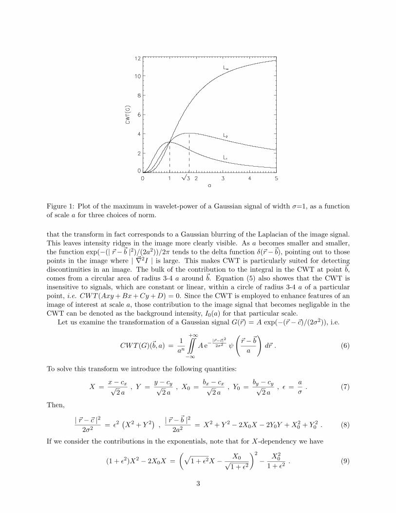
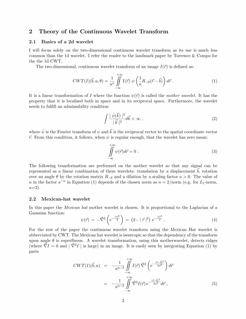
Figure 1: Plot of the maximum in wavelet-power of a Gaussian signal of width σ=1, as a functionof scale a for three choices of norm.
that the transform in fact corresponds to a Gaussian blurring of the Laplacian of the image signal.This leaves intensity ridges in the image more clearly visible. As a becomes smaller and smaller,the function exp(−(| ~r−~b |2)/(2a2))/2π tends to the delta function δ(~r−~b), pointing out to thosepoints in the image where | ~∇2I | is large. This makes CWT is particularly suited for detectingdiscontinuities in an image. The bulk of the contribution to the integral in the CWT at point ~b,comes from a circular area of radius 3-4 a around ~b. Equation (5) also showes that the CWT isinsensitive to signals, which are constant or linear, within a circle of radius 3-4 a of a particularpoint, i.e. CWT (Axy+Bx+Cy+D) = 0. Since the CWT is employed to enhance features of animage of interest at scale a, those contribution to the image signal that becomes negligable in theCWT can be denoted as the background intensity, I0(a) for that particular scale.
Let us examine the transformation of a Gaussian signal G(~r) = A exp(−(~r − ~c)/(2σ2)), i.e.
CWT (G)(~b, a) =1
an
+∞¨
−∞
A e−|~r−~c|2
2σ2 ψ
(
~r −~ba
)
d~r . (6)
To solve this transform we introduce the following quantities:
X =x− cx√
2 a, Y =
y − cy√2 a
, X0 =bx − cx√
2 a, Y0 =
by − cy√2 a
, ǫ =a
σ. (7)
Then,
| ~r − ~c |22σ2
= ǫ2(
X2 + Y 2)
,| ~r −~b |2
2a2= X2 + Y 2 − 2X0X − 2Y0Y +X2
0 + Y 20 . (8)
If we consider the contributions in the exponentials, note that for X-dependency we have
(1 + ǫ2)X2 − 2X0X =
(
√
1 + ǫ2X − X0√1 + ǫ2
)2
− X20
1 + ǫ2. (9)
3
It thus makes sense to change to new variables:
ξ =√
1 + ǫ2X − X0√1 + ǫ2
, ψ =√
1 + ǫ2Y − Y0√1 + ǫ2
. (10)
Then for X (equivalently for Y ):
X =ξ√
1 + ǫ2+
1
1 + ǫ2X0 , X−X0 =
ξ√1 + ǫ2
− ǫ2
1 + ǫ2X0 , ǫ
2X2+(X−X0)2 = ξ2+
ǫ2
1 + ǫ2X2
0 .
(11)Also,
2− | ~r −~b |2a2
= 2− 2(X −X0)2 − 2(Y − Y0)
2
= 2− 2
(
ξ√1 + ǫ2
− ǫ2
1 + ǫ2X0
)2
− 2
(
ψ√1 + ǫ2
− ǫ2
1 + ǫ2Y0
)2
= 2− 2
(
ǫ2
1 + ǫ2
)2(
X20 + Y 2
0
)
+ 4ǫ4
(1 + ǫ2)3/2(X0ξ + Y0ψ)−
2
1 + ǫ2(
ξ2 + ψ2)
.(12)
Finally, with
dxdy = 2a2dXdY =2a2
1 + ǫ2dξdψ , (13)
the transform becomes:
CWT (G)(~b, a) =2A e
−
ǫ2(X2
0+Y
20 )
1+ǫ2
an−2 (1 + ǫ2)
+∞¨
−∞
[
2− 2
(
ǫ2
1 + ǫ2
)2(
X20 + Y 2
0
)
+ 4ǫ4
(1 + ǫ2)3/2(X0ξ + Y0ψ)
− 2
1 + ǫ2(
ξ2 + ψ2)
]
e−ξ2
e−ψ2
dξ dψ . (14)
We make use of the definite integrals
+∞ˆ
−∞
e−αt2
dt =
√
π
α,
+∞ˆ
−∞
te−αt2
dt = 0 ,
+∞ˆ
−∞
t2e−αt2
dt = − ∂
∂α
+∞ˆ
−∞
e−αt2
dt =1
2α
√
π
α. (15)
Hence Eq. (14) becomes
CWT (G)(~b, a) =2πA e
−
ǫ2(X2
0+Y
20 )
1+ǫ2
an−2 (1 + ǫ2)
[
2− 2
(
ǫ2
1 + ǫ2
)2(
X20 + Y 2
0
)
− 2
1 + ǫ2
]
=2πA ǫ2 e
−
ǫ2(X2
0+Y
20 )
1+ǫ2
an−2 (1 + ǫ2)2
[
2− 2ǫ2
1 + ǫ2(
X20 + Y 2
0
)
]
=2πA
an−2
ǫ2
(1 + ǫ2)2
[
2− 2ǫ2
1 + ǫ2(
X20 + Y 2
0
)
]
e−
ǫ2(X2
0+Y
20 )
1+ǫ2
=2πA
an−2
(
aσ
)2
(
1 +(
aσ
)2)2
ψ
(
~b− ~c√a2 + σ2
)
, (16)
4
where we used:ǫ2
1 + ǫ2(
X20 + Y 2
0
)
=a2
a2 + σ2
(
| ~b− ~c |22a2
)
=| ~b− ~c |22(a2 + σ2)
. (17)
For a fixed scale, the maximum value of CWT (G) is reached at ~b = ~c. Let us consider thedependency of CWT (G) as a function of scale a, at that position. This is illustrated in Figure 1.It is clear that for n > 0 (excluding L∞-norm), CWT (G)(~c, a) reaches a maximum at:
am =
√
4
n− 1σ , CWT (G)(~c, am) =
πA
4n2(
4
n− 1
)2−n
2
(18)
For L1-norm, n = 2, this means that the wavelet power has a local maximum, of value πA, at thescale of the signal, i.e. am = σ. For L2-norm, n = 1, the wavelet power has a local maximum ofvalue (9/4
√
(3))πA at the scale am =√3σ. For L∞-norm, n = 0, there is no local maximum in
wavelet power.
2.3 Image noise
The noise in the EIT images is due to two, assumed independent, contributions: photon noise andCCD read-out noise. The photon noise follows from Poisson statistics, for which the average valueµ and variance σ2pn of the photon density distribution are equal to the expectancy value, whichin this case is equal to the part of the photon flux, Φint, interacting with the CCD camera. Weexpress Φint and σpn, originally in units of number of photons, into Digital Number (DN) unitsby multiplying by a factor Nph/d, where Nph is the gain of electrons per photon, equal to 12398 /(3.65 λ) and d is the digitization constant, equal to 16.7 eV per DN for the EIT instrument (Dereet al., 2000). λ is the wavelength bandpass, expressed in Angstroms. The average and variance ofthe CCD read-out noise, σCCD, are assumed constant. The latter is, for nominal EIT observationconditions, equal to 2.7 DN2. The noise variance in the EIT images is written as:
σ2noise(~r) =Nph
dI(~r) + σ2CCD =
203.4
λ(A)I(~r) + 2.7 , (19)
where I corresponds to the image intensity, which is the photon flux in units of DN. The EITinstrument has four possible wavelength bandpasses: 171A, 195A, 284A and 304A. For these fourvalues, the ratio 203.4/λ(A) is equal to 1.19, 1.04, 0.72 and 0.67 respectively.
How does the noise look like in a wavelet transformation? Consider N(~r) to be a functiondescribing the noise contribution to the image intensity. The CWT of N may be approximated bytwo, essentially finite, sums:
CWT (N) ≈∑
i,j
ψi,j Ni,j∆Ai,j , (20)
with ψi,j = ψ(| ~ri,j −~bi,j | /a)/an and Ni,j = N(~ri,j), and where ∆Ai,j = ∆xi,j∆yi,j is the intervalof area, which is chosen small enough as to have the sum approximate the integral. We consider thephoton noise. In this case each Ni,j∆Ai,j has a Poisson distribution with an average and variance,both equal to Nph/d I0(a)i,j∆Ai,j , where I0(a) is the background intensity at scale a. The CWTof the average, < N >, and the variance, σpn, of the noise fluctuations due to photon noise, are
5
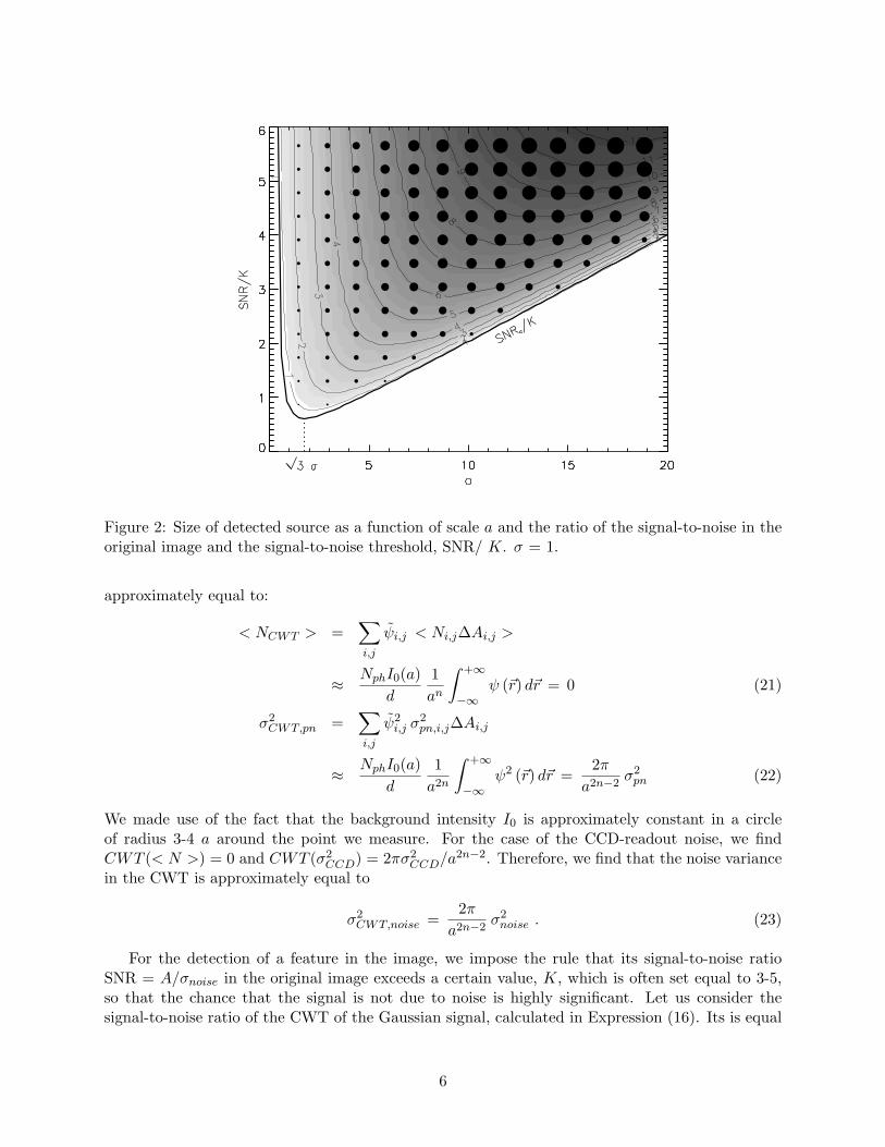
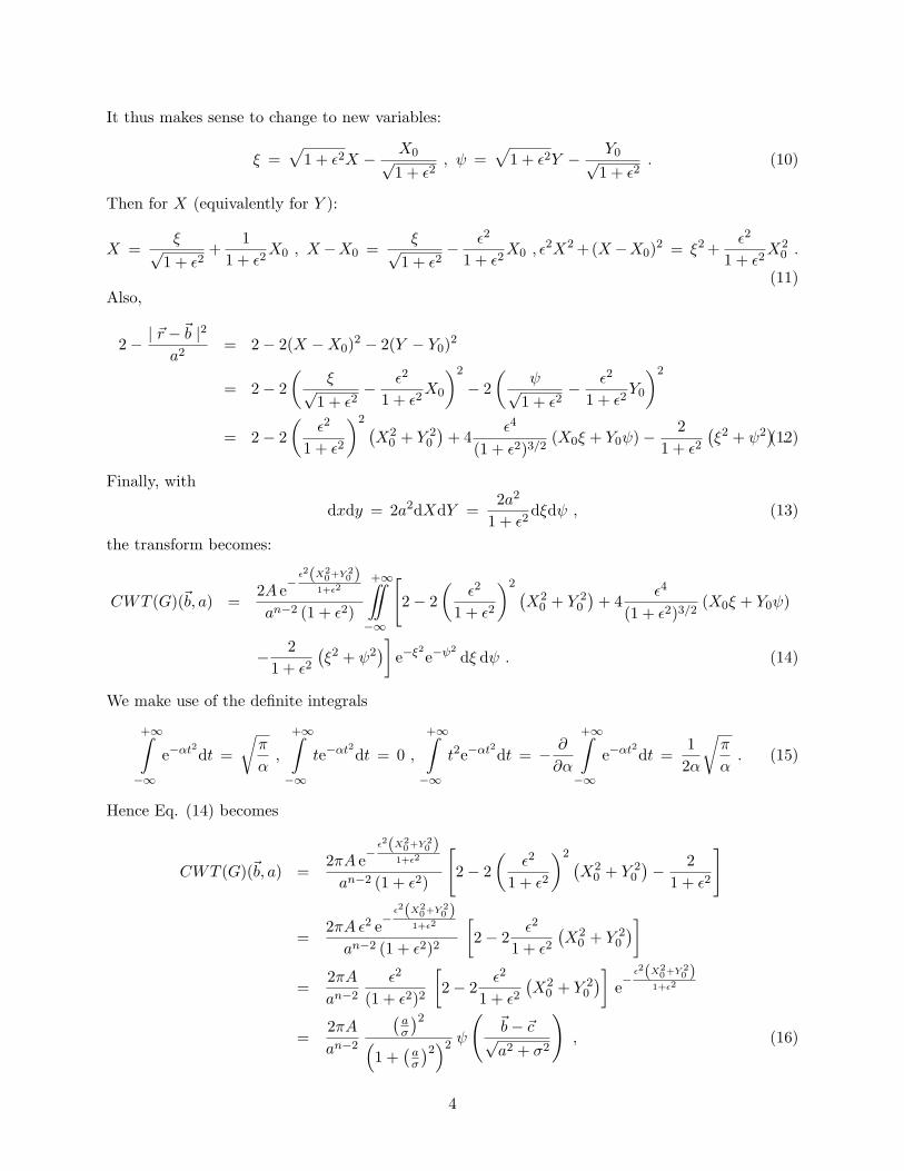
Figure 2: Size of detected source as a function of scale a and the ratio of the signal-to-noise in theoriginal image and the signal-to-noise threshold, SNR/ K. σ = 1.
approximately equal to:
< NCWT > =∑
i,j
ψi,j < Ni,j∆Ai,j >
≈ NphI0(a)
d
1
an
ˆ +∞
−∞
ψ (~r) d~r = 0 (21)
σ2CWT,pn =∑
i,j
ψ2i,j σ
2pn,i,j∆Ai,j
≈ NphI0(a)
d
1
a2n
ˆ +∞
−∞
ψ2 (~r) d~r =2π
a2n−2σ2pn (22)
We made use of the fact that the background intensity I0 is approximately constant in a circleof radius 3-4 a around the point we measure. For the case of the CCD-readout noise, we findCWT (< N >) = 0 and CWT (σ2CCD) = 2πσ2CCD/a
2n−2. Therefore, we find that the noise variancein the CWT is approximately equal to
σ2CWT,noise =2π
a2n−2σ2noise . (23)
For the detection of a feature in the image, we impose the rule that its signal-to-noise ratioSNR = A/σnoise in the original image exceeds a certain value, K, which is often set equal to 3-5,so that the chance that the signal is not due to noise is highly significant. Let us consider thesignal-to-noise ratio of the CWT of the Gaussian signal, calculated in Expression (16). Its is equal
6
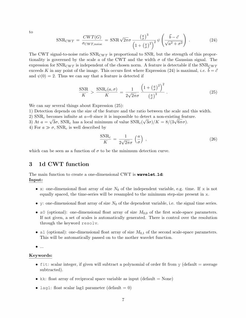
to
SNRCWT =CWT (G)
σCWT,noise= SNR
√2πσ
(
aσ
)3
(
1 +(
aσ
)2)2
ψ
(
~b− ~c√a2 + σ2
)
. (24)
The CWT signal-to-noise ratio SNRCWT is proportional to SNR, but the strength of this propor-tionality is goverened by the scale a of the CWT and the width σ of the Gaussian signal. Theexpression for SNRCWT is independent of the chosen norm. A feature is detectable if the SNRCWT
exceeds K in any point of the image. This occurs first where Expression (24) is maximal, i.e. ~b = ~cand ψ(0) = 2. Thus we can say that a feature is detected if
SNR
K>
SNRc(a, σ)
K=
1
2√2πσ
(
1 +(
aσ
)2)2
(
aσ
)3. (25)
We can say several things about Expression (25):1) Detection depends on the size of the feature and the ratio between the scale and this width.2) SNRc becomes infinite at a=0 since it is impossible to detect a non-existing feature.3) At a =
√3σ, SNRc has a local minimum of value SNRc(
√3σ)/K = 8/(3
√6πσ).
4) For a≫ σ, SNRc is well described by
SNRcK
=1
2√2πσ
(a
σ
)
, (26)
which can be seen as a function of σ to be the minimum detection curve.
3 1d CWT function
The main function to create a one-dimensional CWT is wavelet 1d:Input:
• x: one-dimensional float array of size N0 of the independent variable, e.g. time. If x is notequally spaced, the time-series will be resampled to the minimum step-size present in x.
• y: one-dimensional float array of size N0 of the dependent variable, i.e. the signal time series.
• a0 (optional): one-dimensional float array of size M0,0 of the first scale-space parameters.If not given, a set of scales is automatically generated. There is control over the resolutionthrough the keyword resolv.
• a1 (optional): one-dimensional float array of size M0,1 of the second scale-space parameters.This will be automatically passed on to the mother wavelet function.
• ...
Keywords:
• fit: scalar integer, if given will subtract a polynomial of order fit from y (default = averagesubtracted).
• kk: float array of reciprocal space variable as input (default = None)
• lag1: float scalar lag1 parameter (default = 0)
7
• missing: Boolean stating whether data is missing (default = False)
• mother: string of name of mother wavelet: ’morlet’ (default = ’morlet’)
• regular: Boolean stating whether the intervals in x are regular (default = True) if notregular the data will be interpolated onto a regular grid
• resolv: Scalar of resolution of scales (default = 1.0)
• siglvl: Scalar of significance level between 0 and 1 (default = 0.99)
• variance: Scalar of variance to use in determining significance (default = variance(y)) Notethat if fit is given, the default variance is that of the residual y where the polynomial hasbeen substracted
Output:
C: object containing the following attributes
• C.x0: copy of original one-dimensional float array of size N0 of independent variable x.
• C.y0: copy of original one-dimensional float array of size N0 of dependent variable y.
• C.x: one-dimensional float array of size N of independent variable. Can be of different sizethan C.x0, especially when x0 is not equally-spaced and required resampling.
• C.dxx: float scalar of step-size of C.x
• C.cwt: the complex at least two-dimensional float array of dimension N ×M0 ×M1 × . . . ofthe CWT.
• C.cwt real: real part of CWT.
• C.cwt imag: imaginary part of CWT.
• C.cwt abs: absolute part of CWT
• C.scale: array of scales (first scale-space parameter) in units of indices, either bases oninput or Choice of scales s = s02
jdj with j=0..M0-1, M0 = log2(Ndx/s0)/dj. dj is chosensuch that σ of reciprocal wavelet is larger than scale sampling difference.
• C.period: floating array size M0 of scales (first scale-space parameter) in units of indepen-dent variable. i.e.
• C.coi: float array of size N containing the scale for the cone of influence
• C.signif: array of size M0 of the significance value as a function of scale
• C.siglvl: scalar float of significance level, between 0 and 1.
• C.array missing: int array of size N indicating if data is missing (value=0) or not(value=1).
• C.fft theor: array of size M0 of statistics for significance calculation.
• C.time max: float array of size of C.count max of x-values of maxima in CWT.
8

• C.period max: float array of size C.count max of y-values of maxima in CWT
• C.count max: number of maxima present
• C.mother: string name of mother wavelet used, e.g. ’morlet’
• C.fit: scalar integer of order of polynomial fit (if set).
• C.yfit: float array of size N of polynomial fit.
An example usage syntax is:
C = wavelet 1d(t,y,mother=’morlet’,siglvl=0.99)
which does the same as
C = wavelet 1d(t,y)
The mother wavelet function is given as a function with the name construct wvl func +
mother + 1, e.g. wvl func morlet1. Here, only one mother wavelet is given but others arepossible. The function calculates the mother wavelet in reciprocal (Fourier) space as a function ofk. The function wvl func morlet1 represents the one-dimensional Morlet mother wavelet. Thefunction in principle is never needed to be called separately. It has the following structure:Input:
• kx: float array of size Nk of reciprocal space array
• a0: scalar float of first scale parameter
• a1 (optional): scalar float of second scale parameter
• ...
Keywords:
• norm: Scalar integer of norm used (default = 1)
• epsilon: Scalar float controlling width of wavelet (default = 1.)
• k0: Scalar float controlling number of oscillations underneath envelope (default = 5.6)
Output:
• wavelet: FFT of mother wavelet for given scale as a function of kx
• period: Scalar of period associated with scale a0
• coi: float array containing the scale for the cone of influence
• dofmin: scalar integer of degree of freedom
In the module a plot function is included to easily visualise the result called plot1, with syntax:Input:
• object as output from wavelet 1d.
Keywords:
9
• CWT:
– real: Boolean, plot real part of CWT (default = False)
– imaginary: Boolean, plot imaginary part of CWT (default = False)
– absolute: Boolean, plot absolute part of CWT (default = True)
– zrange: 2-element array of min-max of CWT to plot (default = [min,max])
• Scales:
– freq: Boolean, plot versus frequency = 2 π / C.scale (default = False)
– yrange: 2-element array of scale-range (default = [min,max])
– ylog: Boolean, plot logarithmic scale (defaull = True)
• Colors:
– theme: theme of color scheme: ’blue’,’red’,’’ (default = ’’)
– cmap: colormap used for x-scale plot (default given by theme)
– color: color of lines (default given by theme)
– coi color: color of COI hatches (default givem by theme)
– background color: color of background in time series and power spectrum plots(default given by theme)
• Titles:
– title: title of x-scale plot (default = ’CWT’)
– title scale: title of y-label in x-scale plot (default = ’period’ or ’frequency’)
– title time: title of x-label of time series plot (default = ’time’)
– title signal: title of y-label of time series plot (default = ’signal’)
The demo demo1 shows an example of the usage of wavelet1dandplot1 :import numpy as np
import random
nx = 128
t = np.arange(nx)/(nx-1.) * 10.
w1 = 2.*np.pi/1.9
w2 = 0.5*w1 + t/t.max()*(2.5*w1)
y = np.cos(w1*t) + 2*np.cos(w2*t)
r = np.zeros(nx)
for i in np.arange(nx): r[i] = random.random() * 1.5
y = y + r
C = wavelet_1d(t,y,mother=’morlet’,siglvl=0.9)
fig = plt.figure(num=0,figsize=[8,6],dpi=100,facecolor=’White’,edgecolor=’White’)
plot1(C,freq=False,theme=’Blue’)
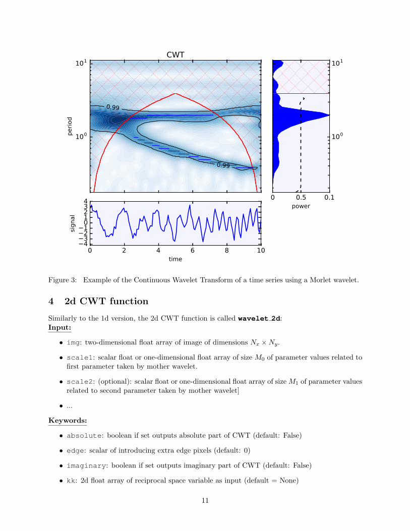
the result of which is shown in Fig. 3, and can be reproduced by running the function demo1.
10
100
101period
0.99
0.99
CWT
0 2 4 6 8 10time
−4−3−2−101234
signal
0 0.5 0.1power
100
101
Figure 3: Example of the Continuous Wavelet Transform of a time series using a Morlet wavelet.
4 2d CWT function
Similarly to the 1d version, the 2d CWT function is called wavelet 2d:Input:
• img: two-dimensional float array of image of dimensions Nx ×Ny.
• scale1: scalar float or one-dimensional float array of size M0 of parameter values related tofirst parameter taken by mother wavelet.
• scale2: (optional): scalar float or one-dimensional float array of sizeM1 of parameter valuesrelated to second parameter taken by mother wavelet]
• ...
Keywords:
• absolute: boolean if set outputs absolute part of CWT (default: False)
• edge: scalar of introducing extra edge pixels (default: 0)
• imaginary: boolean if set outputs imaginary part of CWT (default: False)
• kk: 2d float array of reciprocal space variable as input (default = None)
11
0 10 20 30 40 50 6005
1015202530
original , σ0 = 3
0 10 20 30 40 50 6005
1015202530
scale = 0.34
0 10 20 30 40 50 6005
1015202530
scale = 3.1
0 10 20 30 40 50 6005
1015202530
scale = 8.62
0 2 4 6 8 10scale
0.0
0.2
0.4
0.6
0.8
1.0
Re(C
WT) [a.u.]
scale
=σ0
scale
=√ 3
σ0
norm = 1
norm = 2
norm = ∞
CWT at (32,16)
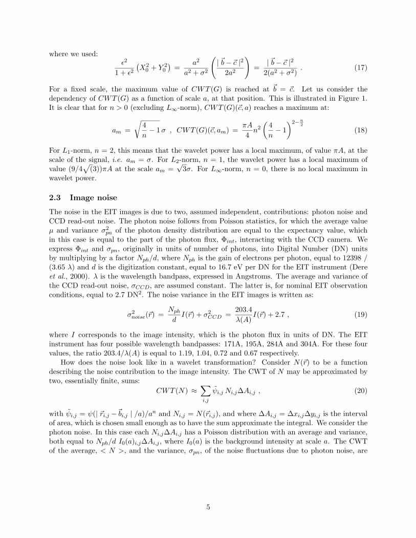
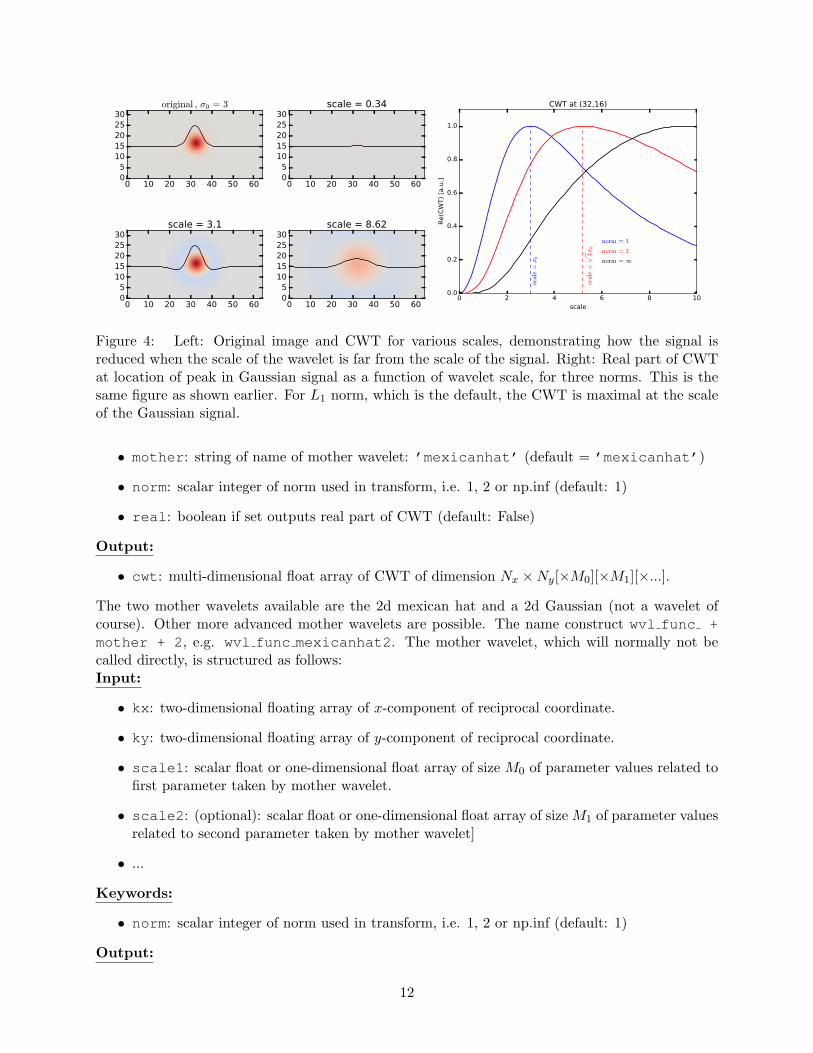
Figure 4: Left: Original image and CWT for various scales, demonstrating how the signal isreduced when the scale of the wavelet is far from the scale of the signal. Right: Real part of CWTat location of peak in Gaussian signal as a function of wavelet scale, for three norms. This is thesame figure as shown earlier. For L1 norm, which is the default, the CWT is maximal at the scaleof the Gaussian signal.
• mother: string of name of mother wavelet: ’mexicanhat’ (default = ’mexicanhat’)
• norm: scalar integer of norm used in transform, i.e. 1, 2 or np.inf (default: 1)
• real: boolean if set outputs real part of CWT (default: False)
Output:
• cwt: multi-dimensional float array of CWT of dimension Nx ×Ny[×M0][×M1][×...].
The two mother wavelets available are the 2d mexican hat and a 2d Gaussian (not a wavelet ofcourse). Other more advanced mother wavelets are possible. The name construct wvl func +
mother + 2, e.g. wvl func mexicanhat2. The mother wavelet, which will normally not becalled directly, is structured as follows:Input:
• kx: two-dimensional floating array of x-component of reciprocal coordinate.
• ky: two-dimensional floating array of y-component of reciprocal coordinate.
• scale1: scalar float or one-dimensional float array of size M0 of parameter values related tofirst parameter taken by mother wavelet.
• scale2: (optional): scalar float or one-dimensional float array of sizeM1 of parameter valuesrelated to second parameter taken by mother wavelet]
• ...
Keywords:
• norm: scalar integer of norm used in transform, i.e. 1, 2 or np.inf (default: 1)
Output:
12
• wavelet: two-dimensional float array of scaled wavelet function in reciprocal space.
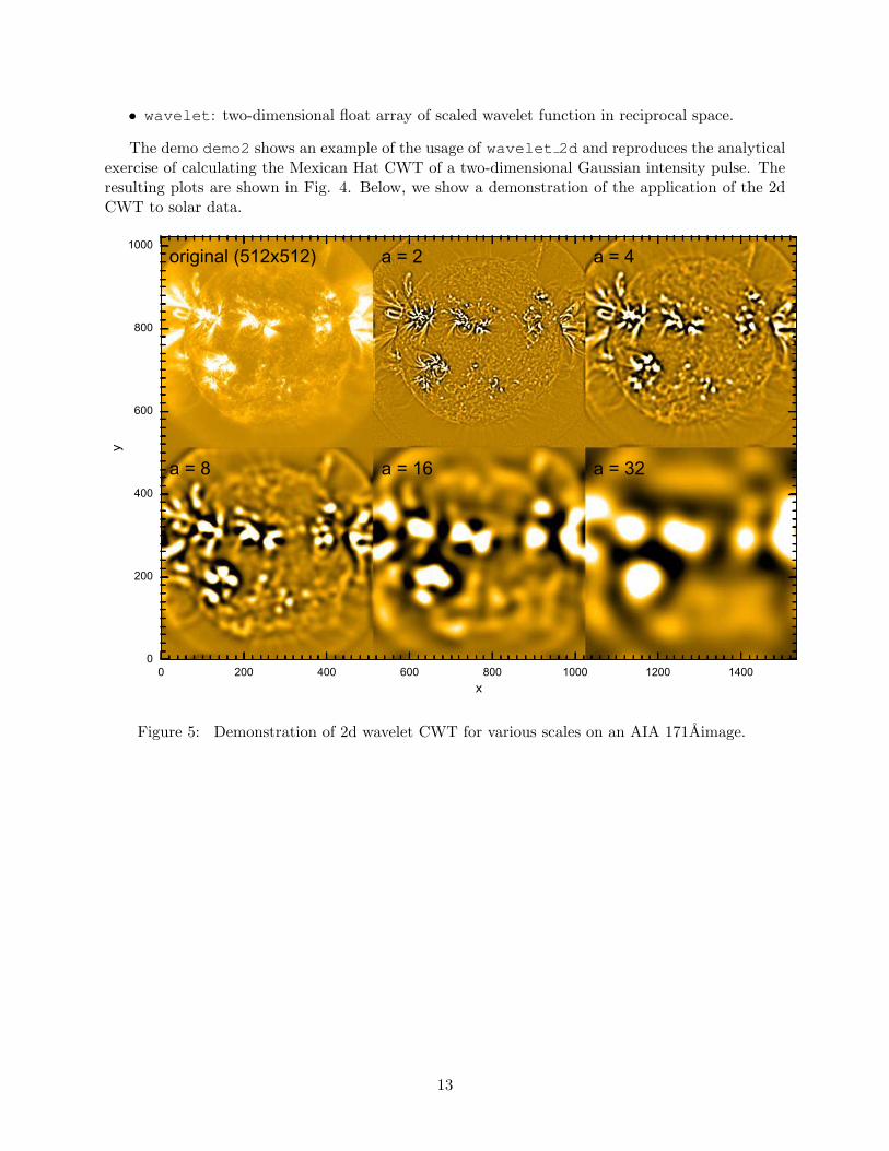
The demo demo2 shows an example of the usage of wavelet 2d and reproduces the analyticalexercise of calculating the Mexican Hat CWT of a two-dimensional Gaussian intensity pulse. Theresulting plots are shown in Fig. 4. Below, we show a demonstration of the application of the 2dCWT to solar data.
0 200 400 600 800 1000 1200 1400x
0
200
400
600
800
1000
y
original (512x512) a = 2 a = 4
a = 8 a = 16 a = 32
Figure 5: Demonstration of 2d wavelet CWT for various scales on an AIA 171Aimage.
13