Embed Size (px)
Citation preview

Continuous Time Structural Equation Modelling
With R Package ctsem
Charles C. Driver
Max Planck Institute for Human DevelopmentJohan H. L. Oud
Radboud University Nijmegen
Manuel C. Voelkle
Humboldt University BerlinMax Planck Institute for Human Development
Abstract
We introduce ctsem (Driver, Oud, and Voelkle in press), an R package for continuoustime structural equation modelling of panel (N > 1) and time series (N = 1) data, us-ing full information maximum likelihood. Most dynamic models (e.g., cross-lagged panelmodels) in the social and behavioural sciences are discrete time models. An assumptionof discrete time models is that time intervals between measurements are equal, and thatall subjects were assessed at the same intervals. Violations of this assumption are oftenignored due to the difficulty of accounting for varying time intervals, therefore parameterestimates can be biased and the time course of effects becomes ambiguous. By usingstochastic differential equations to estimate an underlying continuous process, continuoustime models allow for any pattern of measurement occasions. By interfacing to OpenMx,ctsem combines the flexible specification of structural equation models with the enhanceddata gathering opportunities and improved estimation of continuous time models. ctsemcan estimate relationships over time for multiple latent processes, measured by multiplenoisy indicators with varying time intervals between observations. Within and between ef-fects are estimated simultaneously by modelling both observed covariates and unobservedheterogeneity. Exogenous shocks with different shapes, group differences, higher orderdiffusion effects and oscillating processes can all be simply modeled. We first introduceand define continuous time models, then show how to specify and estimate a range ofcontinuous time models using ctsem.
Keywords: time series, longitudinal modelling, panel data, state space, structural equationmodelling, continuous time, stochastic differential equation, dynamic models, Kalman filter,R.
1. Introduction
Dynamic models, such as the well known vector autoregressive model, are widely used inthe social and behavioural sciences. They allow us to see how fluctuations in processes re-late to later values of those processes, the effect of an input at a particular time, how thevarious factors relate to average levels of the processes, and many other possibilities. Someexamples with panel data include the impact of European institutional changes on business
2 Continuous Time Structural Equation Modelling With ctsem
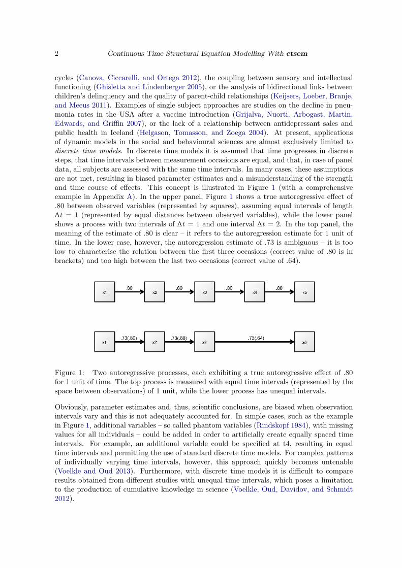
cycles (Canova, Ciccarelli, and Ortega 2012), the coupling between sensory and intellectualfunctioning (Ghisletta and Lindenberger 2005), or the analysis of bidirectional links betweenchildren’s delinquency and the quality of parent-child relationships (Keijsers, Loeber, Branje,and Meeus 2011). Examples of single subject approaches are studies on the decline in pneu-monia rates in the USA after a vaccine introduction (Grijalva, Nuorti, Arbogast, Martin,Edwards, and Griffin 2007), or the lack of a relationship between antidepressant sales andpublic health in Iceland (Helgason, Tomasson, and Zoega 2004). At present, applicationsof dynamic models in the social and behavioural sciences are almost exclusively limited todiscrete time models. In discrete time models it is assumed that time progresses in discretesteps, that time intervals between measurement occasions are equal, and that, in case of paneldata, all subjects are assessed with the same time intervals. In many cases, these assumptionsare not met, resulting in biased parameter estimates and a misunderstanding of the strengthand time course of effects. This concept is illustrated in Figure 1 (with a comprehensiveexample in Appendix A). In the upper panel, Figure 1 shows a true autoregressive effect of.80 between observed variables (represented by squares), assuming equal intervals of length∆t = 1 (represented by equal distances between observed variables), while the lower panelshows a process with two intervals of ∆t = 1 and one interval ∆t = 2. In the top panel, themeaning of the estimate of .80 is clear – it refers to the autoregression estimate for 1 unit oftime. In the lower case, however, the autoregression estimate of .73 is ambiguous – it is toolow to characterise the relation between the first three occasions (correct value of .80 is inbrackets) and too high between the last two occasions (correct value of .64).
Figure 1: Two autoregressive processes, each exhibiting a true autoregressive effect of .80for 1 unit of time. The top process is measured with equal time intervals (represented by thespace between observations) of 1 unit, while the lower process has unequal intervals.
Obviously, parameter estimates and, thus, scientific conclusions, are biased when observationintervals vary and this is not adequately accounted for. In simple cases, such as the examplein Figure 1, additional variables – so called phantom variables (Rindskopf 1984), with missingvalues for all individuals – could be added in order to artificially create equally spaced timeintervals. For example, an additional variable could be specified at t4, resulting in equaltime intervals and permitting the use of standard discrete time models. For complex patternsof individually varying time intervals, however, this approach quickly becomes untenable(Voelkle and Oud 2013). Furthermore, with discrete time models it is difficult to compareresults obtained from different studies with unequal time intervals, which poses a limitationto the production of cumulative knowledge in science (Voelkle, Oud, Davidov, and Schmidt2012).

Charles C. Driver, Johan H. L. Oud, Manuel C. Voelkle 3
Continuous time models overcome these problems, offering researchers the possibility to es-timate parameters free from bias due to unequal intervals, easily compare between studiesand datasets with different observation schedules, gather data with variable time intervalsbetween observations, understand changes in observed effects over time, and parsimoniouslyspecify complex dynamics. Although continuous time models have a long history (Coleman1964; Hannan and Tuma 1979), their use in the social sciences is still uncommon. At least inpart, this is due to a lack of suitable software to specify and estimate continuous time models.With the introduction of ctsem in this article, we want to overcome this limitation. Althoughwe will define continuous time models in the next section and provide several examples in thesections thereafter, a comprehensive treatment of continuous time models is beyond the scopeof this article. For a more general introduction to continuous time models by means of SEM,the reader is referred to Voelkle et al. (2012). For additional information on the technicaldetails we refer the reader to Oud and Jansen (2000).
While there are already a range of packages that deal with continuous time (stochastic dif-ferential equation) models in R, most focus on single subject applications. These include sde
(Iacus 2015), yuima (Brouste, Fukasawa, Hino, Iacus, Kamatani, Koike, Masuda, Nomura,Ogihara, Shimuzu, and others 2014), SIM.DiffProc (Boukhetala and Guidoum 2014), cts
(Wang 2013), POMP (King et al. 2010). For multi-subject approaches, OpenMx (Neale et al.2015) now includes the function mxExpectationStateSpaceContinuousTime, which can becombined with the function mxFitFunctionMultigroup for fixed effects based group analysis.PSM (Klim, Mortensen, Kristensen, Overgaard, and Madsen 2009) has implemented a broadrange of mixed-effects models, but the specification and optimization of models is relativelydemanding in terms of user skill and computational resources. ctsem is focused on providingan accessible workflow for full information maximum likelihood estimation of time series andpanel data based continuous time multivariate autoregressive models with random intercepts.Using ctsem, one may specify: Cross lagged panel models; latent growth curve models; ran-dom intercepts at the latent or manifest level; damped oscillators; dynamic factor analysismodels; constant or time dependent exogenous predictors; continuous time ARMAX modelsfrom the time series tradition; multiple groups or individuals with different parameters; or anycombination of the preceding. First order models should be generally equivalent to discretetime first order models, if there is no variability in time intervals. For an example of thisequivalence in regards to dual change score models see Voelkle and Oud (2015). For an R
script and plot comparing estimates from ctsem and other packages (as well as the use of thectPSMfit function, to fit some models specified using ctsem with PSM), see Appendix B.
The remainder of this article is organised as follows: in Section 2, we provide a formal defini-tion of the continuous time models dealt with in this package. In Section 3 we will show howto install ctsem and give an overview of the package. In Section 4, we will review differentdata structures and discuss the role of time in continuous time models. In Section 5, wewill show how to specify continuous time models in ctsem, followed by a discussion of modelestimation and testing in Section 6. In Section 7 we will discuss various extensions of basiccontinuous time models, including unobserved heterogeneity, time dependent and time inde-pendent exogenous predictors, time series, multiple group models, additional models of thediffusion process, and the analysis of oscillations. We will end with some discussion of variousspecification options and tips for model fitting in Section 8, and point to current limitationsand future research and development directions in Section 9.

4 Continuous Time Structural Equation Modelling With ctsem
2. Continuous time models: fundamentals
The class of continuous time models implemented in ctsem is represented by the multivariatestochastic differential equation:
dηi (t ) =
(
Aηi (t ) + ξi + Bzi +Mχi (t )
)
dt +GdWi (t ) (1)
Vector ηi (t ) ∈ Rv is a v -variable vector of the processes of interest at time t , for subject i. The
matrix A ∈ Rv×v represents the so-called drift matrix, with auto effects on the diagonal andcross effects on the off-diagonals characterising the temporal relationships of the processes.
The long term level of processes ηi (t ) is determined by the v -length vector of random variablesξi , with ξi ∼ N(κ,ϕξ ) for every i, where vector κ ∈ Rv denotes the continuous time intercepts,and matrix ϕξ ∈ R
v×v the covariance across subjects. ξi sets the long-term level of theprocesses and the long-term differences between the processes of individual subjects – withoutit the processes of a stable model would all trend towards zero in the long-run.
The matrix B ∈ Rv×p represents the effect of the p-length vector of (fixed) time independentpredictors z ∈ Rp on processes ηi (t ). Time independent predictors would typically be variablesthat differs between subjects, but are constant within subjects for the time range in question.
Time dependent predictors χi (t ) represent inputs to the system that vary over time and areindependent of fluctuations in the system. Equation 1 shows a generalised form for timedependent predictors, that could be treated a variety of ways dependent on the assumed timecourse (or shape) of time dependent predictors. We use a simple impulse form, in which thepredictors are treated as impacting the processes only at the instant of an observation. Whennecessary, the evolution over time can be modeled by extending the state matrices. This isdemonstrated in the level change example in Section 7.2.2, wherein a model containing onlythe basic impulse has a persistent level change effect added. To achieve the impulse form wereplace part of Equation 1 as follows:
χi (t ) =∑
u ∈Ui
xi,uδ(t − u) (2)
Here, time dependent predictors xi,u ∈ Rl are observed at times u ∈ Ui ⊂ R. The Dirac delta
function δ(t − u) is a generalised function that is ∞ at 0 and 0 elsewhere, yet has an integralof 1 (when 0 is in the range of integration). It is useful to model an impulse to a system, andhere is scaled by the vector of time dependent predictors xi,u . The effect of these impulses onprocesses ηi (t ) is then M ∈ R
v×l .
Wi (t ) ∈ Rv represent independent Wiener processes, with a Wiener process being a random-
walk in continuous time. dWi (t ) is meaningful in the context of stochastic differential equa-tions, and represents the stochastic error term, an infinitesimally small increment of theWiener process. Lower triangular matrix G ∈ Rv×v represents the effect of this noise onthe change in ηi (t ). Q, where Q = GG⊤, represents the variance-covariance matrix of thediffusion process in continuous time.
The solution of the stochastic differential Equation 1 for any time interval t − t0, with t > t0is:

Charles C. Driver, Johan H. L. Oud, Manuel C. Voelkle 5
ηi (t) = eA(t−t0 )ηi (t0) +
A−1[eA(t−t0 ) − I]ξi +
A−1[eA(t−t0 ) − I]Bzi +∫ t
t0
eA(t−s )Mχi (s )ds +
∫ t
t0
eA(t−s )GdWi (s ) (3)
The five summands of this equation correspond to the five of Equation 1, and give the linkbetween the continuous time model and discrete instantiations of the process.
Because we treat time dependent predictors χi as impulses, as shown in Equation 2, theintegral shown in the last but one summand of Equation 3 is easily solved, due to the siftingproperty of the delta function:
∫ t
t0
eA(t−s )Mχi (s )ds =M∑
u ∈Ui∩[t0,t )
eA(t−u )xi,u (4)
The last summand of Equation 3, the integral of the diffusion over the given time interval,exhibits covariance matrix:
cov[
∫ t
t0
eA(t−s )GdWi (s )
]
=
∫ t
t0
eA(t−s )QeA⊤ (t−s )ds = irow
(
A−1# [eA# (t−t0 ) − I] row(Q))
(5)
Where A# = A ⊗ I+ I ⊗A, with ⊗ denoting the Kronecker-product, row is an operation thattakes elements of a matrix rowwise and puts them in a column vector, and irow is the inverseof the row operation.
The process vector ηi (t ) may be directly observed or latent with measurement model
yi (t ) = Γi + Ληi (t ) + ζi (t ), where ζ(t ) ∼ N(0,Θ), and Γ ∼ N(τ,Ψ) (6)
where c-length vector τ is the expected value of Γi , which is distributed across subjectsaccording to covariance matrix Ψ ∈ Rc×c (referred to later as manifest traits – see Section7.1.1). Λ ∈ Rc×v is a matrix of factor loadings, yi (t ) ∈ R
c is a vector of manifest variables,and residual vector ζi ∈ R
c has covariance matrix Θ ∈ Rc×c .
2.1. Continuous time and SEM
Continuous time models have already been implemented as structural equation models, usingeither non-linear algebraic constraints (Oud and Jansen 2000) or linear approximations of thematrix exponential (Oud 2002). Our formulation uses either the SEM RAM (reticular actionmodel) specification as per McArdle and McDonald (1984), or the state space form recentlyadded to OpenMx (Neale et al. 2015; Hunter 2014). For details on the equivalence and differ-ences between SEM and state space modelling techniques, see Chow, Ho, Hamaker, and Dolan

6 Continuous Time Structural Equation Modelling With ctsem
(2010). ctsem translates user specified input matrices and switches into an OpenMx modelconsisting of continuous time parameter matrices, algebraic transformations of these matri-ces to aid optimization (See Section 6), and algebraic transforms from the continuous timeparameters to discrete time parameters for every unique time interval. Expectation matricesare then generated for each individual according to the specified inputs, constraints, and ob-served timing data. Optimization using either the Kalman filter or row-wise full informationmaximum likelihood within OpenMx is used to estimate the parameters.
To see exactly how the various matrices are transformed into a RAM SEM, one may run thefollowing code after ctsem is installed (See Section 3). This example comprises two latentprocesses, three observed indicators, a time dependent predictor, and two time independentpredictors, across three time points of observation.
R> data(✬datastructure✬)
R> datastructure
R> semModel<-ctModel(n.latent=2,n.manifest=3, TRAITVAR=✬auto✬, n.TIpred=2,
+ n.TDpred=1, Tpoints=3, LAMBDA=matrix(c(1,✬lambda21✬, 0, 0,1,0),nrow=3))
R> semFit<-ctFit(datastructure, semModel, nofit=T)
R> semFit$mxobj$A$labels
R> semFit$mxobj$S$labels
R> semFit$mxobj$M$labels
R> semFit$mxobj$F$values
For more detailed information on the specification of continuous time structural equationmodels, the reader is referred to Oud and Jansen (2000); Arnold (1974); Singer (1998); Voelkleet al. (2012). Note that while earlier incarnations of continuous time modelling focusedon approaches to implement the matrix exponential, OpenMx now includes a form of theexponential recommended in computational contexts, the scaling and squaring approach withPade approximation (Higham 2009), which has been implemented in ctsem accordingly.
3. ctsem package overview and installation
As ctsem is an R package, it requires R to be installed, available from www.r-project.org
(R Core Team 2014). The R package OpenMx (Neale et al. 2015) is required, and althoughit will be installed automatically via CRAN if necessary, it is recommended to download itfrom http://openmx.psyc.virginia.edu/. ctsem is available via CRAN, so to install andload within R simply use:
R> install.packages("ctsem")
R> library("ctsem")
Estimating continuous time models via ctsem comprises four steps: First, the data mustbe adequately prepared (Section 4). Then, the continuous time model must be specifiedby creating a ctsem model object using the function ctModel (Sections 5 and 7). Afterspecification, the model must be fit to the data using the function ctFit, after which summary
and plot methods may be used to examine parameter estimates, standard errors, and fitstatistics (Section 6). We will discuss these steps in the following.

Charles C. Driver, Johan H. L. Oud, Manuel C. Voelkle 7
4. Data structure
The internal functions of ctFit use data in a wide layout, with all data for each individual ina single row, including the time intervals between measurement occasions for this individual.Because this is the format used internally when fitting, for the sake of transparency it isalso required as the input format, and is detailed below in Section 4.1. In some cases itmay however be simpler to maintain data in a long format, and use the ctLongToWide andctIntervalise functions we provide to convert from long format with absolute times to wideformat with time intervals. This functionality is discussed in Section 4.2. The choice of timescale and treatment of the initial time point can influence results and will be discussed inSection 4.3, though first time users may find it easier to return to later.
4.1. Wide format
This is the data format required when fitting a model with ctsem. The example data belowdepicts two individuals, observed at three occasions, on three manifest variables, one timedependent predictor, and two time independent predictors. A corresponding path diagram ofone possible model for this data is shown in Figure 2. The data are ordered into blocks asfollows: Manifest process variables, time dependent predictors, time intervals, time indepen-dent predictors. Manifest variables are grouped by measurement occasion and ordered withinthis by variable. In the example there are three manifest variables (Y1, Y2, Y3) assessedacross three measurement occasions. In this case, the first three columns of the data (Y1 T0,Y2 T0, Y3 T0) represent the three manifest variables at the first measurement occasion, timepoint 0, followed by the columns of the second measurement occasion and so on. Note thatmeasurement occasions subsequent to the first may occur at different times for different in-dividuals. Also note the naming convention, wherein the variable name is followed by anunderscore and T, followed by an integer denoting the measurement occasion, beginning atT0. After the manifest variables, any time dependent predictors (there need not be any) aregrouped by variable and ordered within this by measurement occasion. This change of order-ing compared to the dependent variables reflects the fact that relations between exogenouspredictors are not of interest. If they are, then they should instead be included as additionallatent processes. Note also that in continuous time modelling a cause must always precede aneffect in time, precluding instantaneous effects. For this reason, no time dependent predictorsmay be included at the last measurement occasion, because there would be no time for aneffect to occur. In the data below and the model in Figure 2, there is only one time dependentpredictor, TD1, though a second could be added by inserting its two columns directly afterTD1 T1). After the time dependent predictors, T -1 time intervals are specified in chrono-logical order, with column names dT followed by the number of the measurement occasionoccurring after the interval . That is, dT1 refers to the time interval between the first mea-surement occasion, T0, and the second, T1. In continuous time modelling it is imperativeto know the time point at which an observation takes place. Thus, while missing values onobserved scores are no problem, missing values on time intervals are not allowed. Finally, twotime independent predictors (TI1, TI2 – the naming here is only with variable names) arecontained in the last two columns of the data structure.
Y1_T0 Y2_T0 Y3_T0 Y1_T1 Y2_T1 Y3_T1 Y1_T2 Y2_T2 Y3_T2 TD1_T0 TD1_T1 dT1 dT2 TI1 TI2
1 2.5 NA 2.2 2.3 5.1 2.3 4.8 3.9 3.7 0 6.0 4 9 -0.6 -0.6
2 5.6 3.7 5.0 NA 7.0 4.4 2.5 4.6 4.7 0 5.3 1 14 -0.5 -0.2

8 Continuous Time Structural Equation Modelling With ctsem
Figure 2: The first three time points of a two process continuous time model, with threemanifest indicators (blue) measuring 2 latent processes (purple), one time dependent predic-tor(dark green), and two time independent predictors (light green). Variance / covariancepaths are in orange, regressions in red. Light grey paths indicate those that are constrainedto a function of other parameters. Note that the value of parameters for all paths to latentsat time 2 and higher do not directly represent the effect, rather, the effect depends on afunction including the shown parameter and the time interval ∆t. Covariances between thetime dependent predictor and traits (yellow) are not drawn.

Charles C. Driver, Johan H. L. Oud, Manuel C. Voelkle 9
4.2. Conversion from long format with absolute times
Although ctsem uses the wide format as default data input, often data are stored in longformat, that is, each subject has multiple rows of data, with each row reflecting a particu-lar measurement occasion. In addition, time intervals may not be readily available at theindividual level, instead the absolute time when a measurement took place is recorded. Toconvert from long format, the data must contain a subject identification column, columns forevery observed variable, and a time variable. Unlike for the wide format data, at this pointadditional unused variables in the long structure are no problem. In the example below, threemanifest variables of interest (Y1, Y2, Y3) have been observed across a number of occasions,along with one time dependent predictor (TD1) and two time independent predictors (TI1,TI2). The variable ’Time’ contains the time when the measurement took place (e.g., in weeksfrom the beginning of the study).
subject Y1 Y2 Y3 TD1 Time TI1 TI2
[1,] 1 3.13 NA 4.59 0.32625 0 NA -0.609
[2,] 1 2.30 5.11 2.31 -0.00972 1 -0.607 -0.609
[3,] 1 3.85 4.45 NA NA NA NA NA
[4,] 1 3.05 3.02 3.11 -0.26912 2 -0.607 -0.609
[5,] 2 5.26 6.06 5.55 0.07493 3 -0.529 -0.233
[6,] 2 5.68 5.64 7.96 -0.63566 4 -0.529 -0.233
[7,] 2 4.68 5.43 4.79 0.26527 5 -0.529 -0.233
Given the specific wide structure required by ctsem, and that the time points of measurementmay vary across individuals, restructuring from long to wide can be complicated, so we haveincluded functions to manage this. First, the long format data with information on theabsolute time of measurement must be converted to the wide format, using the ctLongToWidefunction (The number of Tpoints in the generated data is also messaged to the user at thispoint, to be used in the next step). Then, subject specific time intervals based on the absolutetime information must be generated, using the function ctIntervalise. One should take carethat the defaults used by ctIntervalise for structuring the data and handling missing timeinformation are appropriate.1
R> data("longexample")
R> wideexample <- ctLongToWide(datalong = longexample, id = "subject",
+ time = "Time", manifestNames = c("Y1", "Y2", "Y3"),
+ TDpredNames = "TD1", TIpredNames = c("TI1", "TI2"))
R> wide <- ctIntervalise(datawide = wideexample, Tpoints = 3, n.manifest = 3,
+ n.TDpred = 1, n.TIpred = 2, manifestNames = c("Y1", "Y2", "Y3"),
+ TDpredNames = "TD1", TIpredNames = c("TI1", "TI2") )
1By default, when timing information is missing, variables measured at that time are also set to NAfor the individual missing the information. Once this is done the actual time of measurement no longerinfluences parameter estimates or likelihood, so we can set it to an arbitrary minimum interval. By default,the mininterval argument to ctIntervalise is set to .001. This argument must be set lower than theminimum time interval recorded in the data, so that later observations can be adjusted without problems.

10 Continuous Time Structural Equation Modelling With ctsem
4.3. Choice of initial time point and time scale
Choice of initial time point: Pre-determined or stationary?
An important aspect of continuous time modelling is the choice of how to handle the initialtime point. In principle, there are two different ways to do so. One approach is to treat thefirst time point as predetermined, where no assumptions are made about the process prior tothe initial time point. In this case, parameters regarding the initial latent variable (latentmeans and variances, and effect of predictors) are freely estimated. This is the default inctsem, though requires some constraining if fitting a single individual.2 When treating thefirst time point as predetermined, it is important to choose a meaningful starting point, asthe process will gradually transition from the variances and means of the initial parameters,towards those of the parameters when the model is stationary. In principle, the initial timepoint does not have to reflect the first measurement occasion, and can also be set to any timeprior. For example it may be of interest to set T0 to the beginning of the school year, althoughthe first measurement was only taken two weeks after start of school. This can be specifiedusing the startoffset argument to ctIntervalise, specifying the amount of time priorto the first observed measurement occasion. The other approach is to assume a stationarymodel, that is, a model where the first observations are merely random instantiations of a longterm process with time-invariant mean and variance expectations. Or, put another way, weassume that sufficient time has elapsed from the unobserved, hypothetical start of the processto our first measurement occasion, such that whatever the start values were, they no longerinfluence the process. Strictly speaking, this requires an infinite length of time, or a processthat began in a stationary state. However, in some practical cases without clear trends inthe data it is possible that the improvement in estimation due to the stationarity assumptionoutweighs related losses (this may also be tested). To implement the stationarity assumptionthe means and variances of the first measurement occasion are constrained according to themodel predicted means and variances across all time points. This is specified by includinga character vector of the T0 matrices to constrain in the ctFit arguments: stationary =
c("T0VAR", "T0MEANS") constrains both means and variances to stationarity. The ctModel
specification of any matrices that are constrained to stationarity is ignored. Note that anybetween-subject variance parameters, factor loadings, manifest residuals, as well as drift anddiffusion parameters, are inherently stationary (given the configuration of ctsem). Morecomplex model specification within ctsem, or direct modification of the generated OpenMx
model, is necessary for modelling time variability in the parameters.
Choice of time scale: Individual or sample relative time?
An additional consideration when treating the first time point as predetermined is necessaryin cases of individually varying time intervals. Here, two alternatives need to be distinguished.The default option is to treat the observation times as relative to the individual, the other isto treat them as relative to the sample. When we treat time as relative to the individual, thefirst observation of every individual is set to measurement occasion T0, even though differentindividuals may have been recorded many years apart. However if we treat time as relative tothe sample, every individual’s observation times are set relative to the very first observationin the entire sample. This may result in a larger and sparser data matrix, potentially with
2Either T0VAR or T0MEANS must be fixed, see Section 7.3.

Charles C. Driver, Johan H. L. Oud, Manuel C. Voelkle 11
only a single observation at the first measurement occasion. To specify sample relative timewhen converting from absolute time to intervals, set the argument individualRelativeTime= FALSE in the ctIntervalise function. The choice between the individual or sample relativetime may influence parameter estimates when the processes are not stationary. One way ofdeciding between the two may be to observe whether the changes of the individuals’ processesis more closely aligned with the sample relative or individual relative time. The changein processes may be more aligned with individual relative time when we expect that theactivity of measurement relates to changes in the process. Consider for instance the relationbetween abstinence behaviour and mood among individuals attending an alcohol addictionclinic. Different individuals may come and go from the clinic over many years, but the meanlevel of abstinence is likely related to when each individual began attending the clinic andbeing measured – not the specific date the observation took place. In contrast, sample relativetime could be more appropriate for a study of linguistic abilities in a cohort of schoolchildrenover the years, with some individuals observed early and some only observed later, once theyare older and more developed. In this case, we may expect changes in the average linguisticability related to sample time. Another example that becomes conveniently available withcontinuous time models and these functions is to arrange the data in individual relative fashionbut using age as the timing variable. In this case, age-related developmental trajectoriesmay be studied. When considering these options one should be aware that consistent up ordown trends over time may confound dynamic parameter estimates, if the innovation (latentresidual) at t is correlated with the process at t − 1. Pre-processing approaches that removetrend components, such as controlling for age or year, removing a linear trend, or differencingscores, may provide some check on model estimates, but the ramifications of these should becarefully considered. Alternatively one may wish to explicitly model the diffusion process,discussed in Section 7.5.
5. Model specification
Continuous time models are specified via the ctModel function. This function takes as inputa series of arguments and parameter matrices, and outputs a list object containing matricesto be later evaluated by the ctFit function. The ctModel function contains many defaultsthat should be generally applicable and safe, in that most parameters are specified to befreely estimated, with a few exceptions.3 However, as with all default settings, they shouldbe checked as they may not be applicable. The arguments to the ctModel function and therelation to equations in Section 2 are shown in Table 1 (required specification) and Table 2(optional specification). The matrices can be specified with either character labels, to indicatefree parameter names, or numeric values, which indicate fixed values. A mixture of both inone matrix is fine. These generally need to be set when constraining parameters to equality(same character label), when fixing certain parameters to specific values (for instance, whenyou do not wish to have a certain parameter in the model, or when testing if an effect isdifferent from 0), or when assigning non-standard names to output parameters.
An example model specification relying heavily on the defaults is:
3ctModel defaults that may not be considered safe, as they are not freely estimated, are the MANIFEST-
MEANS, TRAITVAR and MANIFESTTRAITVAR matrices. These were set to ensure that the defaults areappropriate also for single indicator and N = 1 cases, and because generally only one of the two trait matricescan be set at once. See Section 7.3 regarding manifest means, and Section 7.1.1 regarding the trait matrices.

12 Continuous Time Structural Equation Modelling With ctsem
Argument Sign Meaning
n.manifest c Number of manifest indicators per individual at each measurement occasion.n.latent v Number of latent processes.Tpoints Number of time points, or measurement occasions, in the data.LAMBDA Λ n.manifest × n.latent loading matrix relating latent to manifest variables.
Table 1: Required arguments for ctModel.
Argument Sign Default Meaning.
manifestNames Y1, Y2, etc n.manifest length character vector of manifest names.latentNames eta1, eta2, etc n.latent length character vector of latent names.T0VAR free lower triangular n.latent × n.latent Cholesky matrix of latent
process initial variance / covariance.T0MEANS free n.latent × 1 matrix of latent process means at first time point,
T0.MANIFESTMEANS τ 0 n.manifest × 1 matrix of manifest means.MANIFESTVAR Θ free diag lower triangular n.manifest × n.manifest Cholesky matrix of
variance / covariance between manifests (i.e., measurementerror).
DRIFT A free n.latent × n.latent matrix of continuous auto and cross effects.CINT κ free n.latent × 1 matrix of continuous intercepts.DIFFUSION Q free lower triangular n.latent × n.latent Cholesky matrix of diffu-
sion variance / covariance.TRAITVAR ϕξ NULL NULL if no trait variance, or lower triangular n.latent ×
n.latent Cholesky matrix of trait variance / covariance.MANIFESTTRAITVAR Ψ NULL NULL if no trait variance on manifest indicators, or lower
triangular n.manifest × n.manifest Cholesky matrix.n.TDpred l 0 Number of time dependent predictors in the dataset.TDpredNames TD1, TD2, etc n.TDpred length character vector of time dependent predictor
names.TDPREDMEANS free n.TDpred × (Tpoints-1) rows × 1 column matrix of time de-
pendent predictor means.TDPREDEFFECT M free n.latent × n.TDpred matrix of effects from time dependent
predictors to latent processes.T0TDPREDCOV free n.latent × ((Tpoints-1) × n.TDpred) covariance matrix be-
tween latents at T0 and time dependent predictors.TDPREDVAR free lower triangular (n.TDpred × (Tpoints-1)) × (n.TDpred ×
(Tpoints-1)) Cholesky matrix for time dependent predictorsvariance / covariance.
TRAITTDPREDCOV free n.latent rows × (n.TDpred × (Tpoints-1)) columns covariancematrix for latent traits and time dependent predictors.
TDTIPREDCOV free (n.TDpred × (Tpoints-1)) rows × n.TIpred columns covari-ance matrix between time dependent and independent pre-dictors.
n.TIpred p 0 Number of time independent predictors.TIpredNames TI1, TI2, etc n.TIpred length character vector of time independent predic-
tor names.TIPREDMEANS free n.TIpred × 1 matrix of time independent predictor means.TIPREDEFFECT B free n.latent × n.TIpred effect matrix of time independent predic-
tors on latent processes.T0TIPREDEFFECT free n.latent × n.TIpred effect matrix of time independent predic-
tors on latents at T0.TIPREDVAR free lower triangular n.TIpred × n.TIpred Cholesky matrix of time
independent predictors variance / covariance.startValues NULL a named vector, where the names of each value must match
a parameter in the specified model, and the value sets thestarting value for that parameter during optimization.
Table 2: Optional arguments for ctModel.
Charles C. Driver, Johan H. L. Oud, Manuel C. Voelkle 13
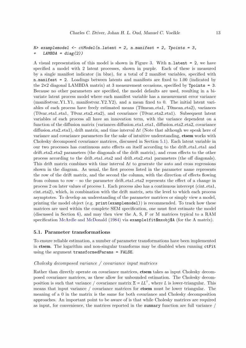
R> examplemodel <- ctModel(n.latent = 2, n.manifest = 2, Tpoints = 3,
+ LAMBDA = diag(2))
A visual representation of this model is shown in Figure 3. With n.latent = 2, we havespecified a model with 2 latent processes, shown in purple. Each of these is measuredby a single manifest indicator (in blue), for a total of 2 manifest variables, specified withn.manifest = 2. Loadings between latents and manifests are fixed to 1.00 (indicated bythe 2×2 diagonal LAMBDA matrix) at 3 measurement occasions, specified by Tpoints = 3.Because no other parameters are specified, the model defaults are used, resulting in a bi-variate latent process model where each manifest variable has a measurement error variance(manifestvar Y1 Y1, manifestvar Y2 Y2), and a mean fixed to 0. The initial latent vari-ables of each process have freely estimated means (T0mean eta1, T0mean eta2), variances(T0var eta1 eta1, T0var eta2 eta2), and covariance (T0var eta2 eta1). Subsequent latentvariables of each process all have an innovation term, with the variance dependent on afunction of the diffusion matrix (variances diffusion eta1 eta1, diffusion eta2 eta2, covariancediffusion eta2 eta1), drift matrix, and time interval ∆t (Note that although we speak here ofvariance and covariance parameters for the sake of intuitive understanding, ctsem works withCholesky decomposed covariance matrices, discussed in Section 5.1). Each latent variable inour two processes has continuous auto effects on itself according to the drift eta1 eta1 anddrift eta2 eta2 parameters (the diagonals of the drift matrix), and cross effects to the otherprocess according to the drift eta1 eta2 and drift eta2 eta1 parameters (the off diagonals).This drift matrix combines with time interval ∆t to generate the auto and cross regressionsshown in the diagram. As usual, the first process listed in the parameter name representsthe row of the drift matrix, and the second the column, with the direction of effects flowingfrom column to row – so the parameter drift eta1 eta2 represents the effect of a change inprocess 2 on later values of process 1. Each process also has a continuous intercept (cint eta1,cint eta2), which, in combination with the drift matrix, sets the level to which each processasymptotes. To develop an understanding of the parameter matrices or simply view a model,printing the model object (e.g. print(examplemodel)) is recommended. To track how thesematrices are used within the complete SEM specification, one must first estimate the model(discussed in Section 6), and may then view the A, S, F or M matrices typical to a RAMspecification McArdle and McDonald (1984) via example1fit$mxobj$A (for the A matrix).
5.1. Parameter transformations
To ensure reliable estimation, a number of parameter transformations have been implementedin ctsem. The logarithm and non-singular transforms may be disabled when running ctFit
using the argument transformedParams = FALSE.
Cholesky decomposed variance / covariance input matrices
Rather than directly operate on covariance matrices, ctsem takes as input Cholesky decom-posed covariance matrices, as these allow for unbounded estimation. The Cholesky decom-position is such that variance / covariance matrix Σ = LL⊤, where L is lower-triangular. Thismeans that input variance / covariance matrices for ctsem must be lower triangular. Themeaning of a 0 in the matrix is the same for both covariance and Cholesky decompositionapproaches. An important point to be aware of is that while Cholesky matrices are requiredas input, for convenience, the matrices reported in the summary function are full variance /

14 Continuous Time Structural Equation Modelling With ctsem
Figure 3: A two process continuous time model with manifest indicators (blue) measuringlatent processes (purple). Variance / covariance paths are in orange, regressions in red.Light grey paths indicate those that are either fixed to certain values or constrained to otherparameters. Note that the value of the parameters for all paths to latents at time 2 and higherdo not directly represent the effect, rather, the effect depends on a function of the shownparameter and the time interval ∆t. This model includes neither observed or unobservedbetween person variance, nor any time dependent predictors.

Charles C. Driver, Johan H. L. Oud, Manuel C. Voelkle 15
covariance matrices. These can be converted to the Cholesky decomposed form using code inthe form t(chol(summary(ctfitobj)$varcovmatrix)).
Logarithmic transforms
While not affecting interpretations of the matrix input or output, internally, by default ctsemoptimizes over the natural logarithm of the diagonal of variance / covariance matrices, and thenatural logarithm of the negative diagonal of the DRIFT matrix. These transformations arereflected in the raw OpenMx parameter output section of the output summary, but otherwiserequire no specific knowledge or action – the transformations all take place internally, and theregular DRIFT and variance / covariance matrices are displayed in the summary matrices.The main limitation imposed by these transforms is that DRIFT diagonals are constrained tobe negative. Although this should be beneficial for most purposes, if one wishes to estimatean unstable (no asymptote) process, this can still be achieved by augmenting the modelspecification with one or more additional latents, or switching parameter transforms off withtransformedParams = FALSE.
Non-singular matrices
To avoid problems with singular matrices, internally, the matrix negDRIFTlog 0.00001 addedto the diagonal elements, while DIFFUSIONlogchol diagonals have .00001 subtracted. Thisensures that DRIFT diagonals are always negative and DIFFUSION diagonals are alwayspositive. When values outside these bounds are input by the user (either as fixed or startingvalues), the values are adjusted as necessary and the user is informed.
6. Model estimation
The ctFit function estimates the specified model, calling the data in wide format along withthe ctsemmodel object. For an example, we can fit a similar model to that defined in Section 5.We first load an example dataset contained in the ctsem package, then use the ctFit functionfor parameter estimation. Output information can be obtained via the summary function. Thedataset used in this example, is a simulation of the relation between leisure time and happinessfor 100 individuals across 6 measurement occasions. Because our data here does not use thedefault manifest variable names of Y1 and Y2, but rather LeisureTime and Happiness, wemust include a manifestNames character vector in our model specification. Because eachmanifest directly measures a latent process, we can use the same character vector for thelatentNames argument, though one could specify any character vector of length 2 here, orrely on the defaults of eta1 and eta2.
R> data("ctExample1")
R> example1model <- ctModel(n.latent = 2, n.manifest = 2, Tpoints = 6,
+ manifestNames = c("LeisureTime", "Happiness"),
+ latentNames = c("LeisureTime", "Happiness"), LAMBDA = diag(2))
R> example1fit <- ctFit(datawide = ctExample1, ctmodelobj = example1model)
The output of summary after fitting such a model includes the matrices representing the con-tinuous time parameters (e.g., DRIFT), a list of estimates of only the free parameters, and fit

16 Continuous Time Structural Equation Modelling With ctsem
information from the OpenMx summary function. Further information can be obtained usingthe argument verbose=TRUE, which will return the raw (by default, transformed) OpenMx
parameter values and standard errors, as well as additional summary matrices of discrete timetransformations for the time interval ∆t = 1 (e.g., discreteDRIFT), and when appropriate,asymptotic values for the parameters as the time interval ∆t approaches ∞ (e.g., asymDIF-FUSION may be taken to represent the total within subject variance of a process). Whenappropriate, standardised matrices are also output with the suffix ‘std’.4
R> summary(example1fit, verbose = TRUE)["discreteDRIFTstd"]
$discreteDRIFTstd
LeisureTime Happiness
LeisureTime 0.9728 -0.0499
Happiness -0.0138 0.9146
The output above shows the standardised discrete time equivalent of the DRIFT matrix fortime interval ∆t = 1. This is provided for convenience, but one should note that it only rep-resents the temporal effects given the specific interval of 1 unit of time (The specific intervalshown for the discrete summary matrices may be modified with the argument timeInterval).The unstandardised discreteDRIFT matrix may be calculated from the continuous drift ma-trix for any desired interval. The following code shows this calculation for a time interval of2.5:
R> expm(summary(example1fit)$DRIFT * 2.5)
See Equation 3 to understand how this arises. From the diagonals of the discreteDRIFTstdmatrix we see that changes in the amount of leisure time one has tend to persist longer(indicated by a higher autoregression) than happiness. The cross-regression in row 2 column1 suggests that as leisure time increases, this tends to be followed by decreases in happiness.Similarly, the cross-regression in row 1 column 2 suggests that as happiness increases, thistends to be followed by decreases in leisure time. While these results are accurate for thespecified model, the specified model is likely inappropriate for this data, which we explainmore of in Section 7.1.1 on unobserved heterogeneity.
6.1. Comparing different models
Suppose we wanted to test the model we fit above against a model where the effect of happinesson later leisure time (parameter drift LeisureTime Happiness) was constrained to 0. First wespecify and fit the model under the null hypothesis by taking our previous model and fixingthe desired parameter to 0:
R> testmodel <- example1model
R> testmodel$DRIFT[1, 2] <- 0
R> testfit <- ctFit(datawide = ctExample1, ctmodelobj = testmodel)
4Standardisations are based on only the relevant variance, not the total. For instance, DRIFT parametersare standardised using only the within-subject variance, asymDIFFUSION, because DRIFT parameters aretypically intended to represent individual, or average individual, temporal dynamics.

Charles C. Driver, Johan H. L. Oud, Manuel C. Voelkle 17
The result may then be compared to the original model with a likelihood ratio test, using theOpenMx function mxCompare. To use this function a base model fit object and a comparisonmodel fit object must be specified, with the latter being a constrained version of the former.Note that ctsem stores the original OpenMx fit object under a $mxobj sub-object, which mustbe referenced when using OpenMx functions directly.
R> mxCompare(example1fit$mxobj, testfit$mxobj)
base comparison ep minus2LL df AIC diffLL diffdf p
1 ctsem <NA> 16 4177 1184 1809 NA NA NA
2 ctsem ctsem 15 4197 1185 1827 19.9 1 0.00000833
According to the conventional p < .05 criterion, results show that the more constrained modelfits the data significantly worse, that is, happiness has a significant effect on later leisure timefor this model and data. An alternative to this approach is to estimate likelihood based 95%confidence intervals for our parameters of interest, from our already fit model:
R> example1cifit <- ctCI(example1fit, confidenceintervals = "DRIFT")
lbound estimate ubound note
ctsem.DRIFT[1,1] -0.0468 -0.0280 -0.01247
ctsem.DRIFT[2,1] -0.0312 -0.0111 0.00869
ctsem.DRIFT[1,2] -0.1083 -0.0697 -0.03775
ctsem.DRIFT[2,2] -0.1485 -0.0896 -0.04595
Now the summary function reports 95% confidence bounds for the continuous drift param-eters, which in case of drift Happiness LeisureTime (DRIFT[1,2]) does not include 0. Forcomplicated models, the estimation of confidence intervals may increase computation timeconsiderably. Note that although the standard errors of parameter estimates may be au-tomatically returned via OpenMx and displayed via summary, verbose = TRUE, likelihoodbased confidence intervals or model comparisons are recommended for hypothesis testing,because confidence intervals may not be symmetric around the point estimate for many pa-rameters in a continuous time model.
6.2. Plots
A visual depiction of the relationships between the processes over time is given by the plot
function for any fit object created by ctFit. This will show the processes’ mean trajectories,within-subject variance, autoregression, and cross regression plots, as well as plots showingexpected changes in each process given either an observed change of 1.00, or an exogenous inputof 1.00 (The former is a mixture of the DIFFUSION and DRIFT matrices, while the latteris just an alternative representation of the auto and cross regression plots). Autoregressionplots show the impact of a 1 unit change in a process on later values of that process, whilecross regression plots show the impact of a 1 unit change in one process on later values ofother processes. Some examples can be seen in Figure 4.

18 Continuous Time Structural Equation Modelling With ctsem
7. Continuous time models: extensions
7.1. Unobserved heterogeneity
Traits at the latent level
When modelling panel data, the continuous intercept parameter κ reflects the expected valuefor continuous time intercept ξ, which determines the average level of a process. In panel data,however, it is common that individuals exhibit stable differences in the level. Within ctsem
we call such stable differences traits, but they may also be thought of more abstractly as unitlevel or between subject differences, or unobserved heterogeneity. Fitting a model that fails toaccount for it will result in parameter estimates that will not reflect the processes of individualsubjects, but will mix between and within-person information (Balestra and Nerlove 1966; Oudand Jansen 2000; Halaby 2004). To avoid this bias, individual differences can be incorporatedin two different ways. One way is to control for observed covariates as will be discussed inSection 7.2.1. However as covariates are likely to be insufficient, one may also estimate thelatent trait variance by estimating the variance and covariance ϕξ of the intercept parameters
ξ across individuals.5 In ctsem, freely estimated latent trait variances and covariances maybe added with the argument TRAITVAR = "auto" to the ctModel command. If the user isinterested in a specific variance-covariance structure, it is of course also possible to specify then.latent × n.latent lower-triangular matrix of free or fixed parameters by hand. To illustratethe inclusion of trait variance, we fit the same model on simulated leisure time and happinessintroduced above, but also model the traits.
R> data("ctExample1")
R> traitmodel <- ctModel(n.manifest = 2, n.latent = 2, Tpoints = 6,
+ LAMBDA = diag(2), manifestNames = c("LeisureTime", "Happiness"),
+ latentNames = c("LeisureTime", "Happiness"), TRAITVAR = "auto")
R> traitfit <- ctFit(datawide = ctExample1, ctmodelobj = traitmodel)
From Figure 4, we can see that after accounting for differences in the trait levels of leisuretime and happiness, the estimated auto and cross regression effects between latent processesare very different. Auto effects (persistence) have reduced, and the magnitude and sign of thecross effects have switched. Now, rather than a decrease in leisure time predicting an increasein happiness, after controlling for unobserved heterogeneity we see instead that increases inleisure time predict later increases in happiness.
Traits at the indicator level
Beyond differences in the level of the latent process, it is also possible that stable individualdifferences in the level of some or all indicators of a process may exist, and as such may bebetter accounted for at the measurement level. Take for instance a latent process, happiness,
5Note that this is a substantially different approach to achieve unbiased effect estimates than the fixed effects
approach (see for example Mundlak 1978), as our SEM specification, while a random effects model which haveat times been associated with bias for within effects, allows unbiased estimation of within and between effectsat the same time. For further details on the estimation of unobserved heterogeneity in an SEM context, seeBollen and Brand (2010), and in the continuous time case Voelkle, Driver, and Oud (2015).

Charles C. Driver, Johan H. L. Oud, Manuel C. Voelkle 19
0 5 10 15 20
0.0
0.4
0.8
Autoregression
Val
ue
drift_LeisureTime_LeisureTimedrift_Happiness_Happiness
0 5 10 15 20
−1.
00.
00.
51.
0
Standardised crossregression
Val
ue
drift_Happiness_LeisureTimedrift_LeisureTime_Happiness
0 5 10 15 20
0.0
0.4
0.8
Autoregression
Val
ue
drift_LeisureTime_LeisureTimedrift_Happiness_Happiness
0 5 10 15 20
−1.
00.
00.
51.
0
Standardised crossregression
Val
ue
drift_Happiness_LeisureTimedrift_LeisureTime_Happiness
Figure 4: Top row shows parameter plots without accounting for trait variance, bottom rowwith trait variance accounted for.
estimated using three survey questions at 10 time points for multiple individuals. The meansfor question one are fixed to 0 to identify the model, while those for questions two and three are2.50 and 1.20 respectively. According to the models we have described so far, the estimated (orfixed) manifest means apply equally to all individuals, and deviations from this are taken torepresent genuine information about the latent process. However, consider that question threequeries happiness with work, which may for some people be consistently high, independent oftheir actual latent happiness, and for some may be consistently low. Calculating the latentprocess using the same mean for happiness with work again confounds between and withinperson information, but we can account for this by using what we will refer to as manifesttraits – an additional, time invariant variance-covariance structure on the measurement level.These are specified by including the MANIFESTTRAITVAR matrix in the ctModel specification,either as MANIFESTTRAITVAR = "auto" wherein time invariant variance and covariance forall indicators is freely estimated, or the n.manifest × n.manifest lower-triangular matrix canbe specified explicitly as usual. Such a specification may allow for improved fit of factormodels, more realistic estimates of the dynamics of individual processes, and the testing ofmeasurement related hypotheses. Note however that identifying restrictions will be necessaryfor any model that contains both manifest and process level traits – one possible form for thismay be a free process level TRAITVAR matrix and a MANIFESTTRAITVAR matrix thatis fixed to 0 across factors, but free within any factors that are measured by more than oneindicator.

20 Continuous Time Structural Equation Modelling With ctsem
7.2. Predictors
ctsem allows the inclusion of time independent as well as time time dependent exogenouspredictors. Time independent predictors could be variables such as gender, personality orsocio-demographic background variables that remain constant over time. An example of atime dependent predictor could be a financial crisis, which all individuals in the sample ex-perience at the same time, or the death of a loved one, which only some individuals mayexperience and for whom the time point of the event may differ. Both events may be thoughtof as adding some relatively distinct and sudden change to an individual’s life, which influencesthe processes of interest. Time dependent predictors are distinguished from the endogenouslatent processes in that they are assumed to be independent of fluctuations in the processes –changes in the latent processes do not lead to changes in the predictor. Furthermore, no tem-poral structure between different time points is modeled. Because of these two assumptions,in any case where the time dependent predictor depends on earlier values of either itself orthe latent process, it may be better to model it as an additional latent process.
Time independent predictors
Time independent predictors are added by including the data as per the structures shownin Section 4, and specifying the number of time independent predictors, n.TIpred, in thectModel arguments. If not using the default variable naming, a TIpredNames charactervector should also be specified. For an example, we add the ‘number of close friends’ as a timeindependent predictor to the earlier leisure time and happiness model. Note that, just like inany conventional regression analysis, if time independent predictors are not centered around0, the estimate of continuous intercept parameters depends on the mean of the predictor.
R> data("ctExample1TIpred")
R> tipredmodel <- ctModel(n.manifest = 2, n.latent = 2, n.TIpred = 1,
+ manifestNames = c("LeisureTime", "Happiness"),
+ latentNames = c("LeisureTime", "Happiness"),
+ TIpredNames = "NumFriends",
+ Tpoints = 6, LAMBDA = diag(2), TRAITVAR = "auto")
R> tipredfit <- ctFit(datawide = ctExample1TIpred, ctmodelobj = tipredmodel)
R>
R> summary(tipredfit, verbose = TRUE)["TIPREDEFFECT"]
R> summary(tipredfit, verbose = TRUE)["discreteTIPREDEFFECT"]
R> summary(tipredfit, verbose = TRUE)["asymTIPREDEFFECT"]
R> summary(tipredfit, verbose = TRUE)["addedTIPREDVAR"]
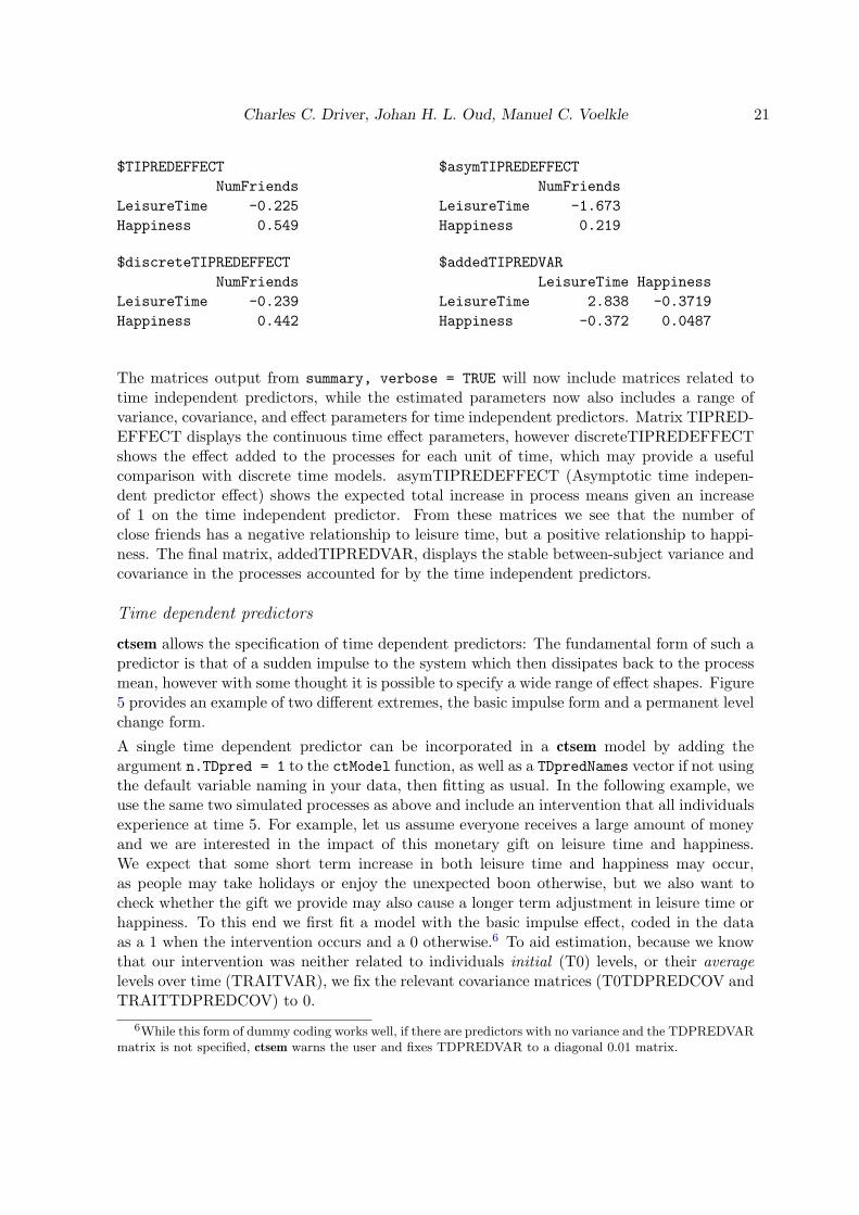
Charles C. Driver, Johan H. L. Oud, Manuel C. Voelkle 21
$TIPREDEFFECT
NumFriends
LeisureTime -0.225
Happiness 0.549
$discreteTIPREDEFFECT
NumFriends
LeisureTime -0.239
Happiness 0.442
$asymTIPREDEFFECT
NumFriends
LeisureTime -1.673
Happiness 0.219
$addedTIPREDVAR
LeisureTime Happiness
LeisureTime 2.838 -0.3719
Happiness -0.372 0.0487
The matrices output from summary, verbose = TRUE will now include matrices related totime independent predictors, while the estimated parameters now also includes a range ofvariance, covariance, and effect parameters for time independent predictors. Matrix TIPRED-EFFECT displays the continuous time effect parameters, however discreteTIPREDEFFECTshows the effect added to the processes for each unit of time, which may provide a usefulcomparison with discrete time models. asymTIPREDEFFECT (Asymptotic time indepen-dent predictor effect) shows the expected total increase in process means given an increaseof 1 on the time independent predictor. From these matrices we see that the number ofclose friends has a negative relationship to leisure time, but a positive relationship to happi-ness. The final matrix, addedTIPREDVAR, displays the stable between-subject variance andcovariance in the processes accounted for by the time independent predictors.
Time dependent predictors
ctsem allows the specification of time dependent predictors: The fundamental form of such apredictor is that of a sudden impulse to the system which then dissipates back to the processmean, however with some thought it is possible to specify a wide range of effect shapes. Figure5 provides an example of two different extremes, the basic impulse form and a permanent levelchange form.
A single time dependent predictor can be incorporated in a ctsem model by adding theargument n.TDpred = 1 to the ctModel function, as well as a TDpredNames vector if not usingthe default variable naming in your data, then fitting as usual. In the following example, weuse the same two simulated processes as above and include an intervention that all individualsexperience at time 5. For example, let us assume everyone receives a large amount of moneyand we are interested in the impact of this monetary gift on leisure time and happiness.We expect that some short term increase in both leisure time and happiness may occur,as people may take holidays or enjoy the unexpected boon otherwise, but we also want tocheck whether the gift we provide may also cause a longer term adjustment in leisure time orhappiness. To this end we first fit a model with the basic impulse effect, coded in the dataas a 1 when the intervention occurs and a 0 otherwise.6 To aid estimation, because we knowthat our intervention was neither related to individuals initial (T0) levels, or their averagelevels over time (TRAITVAR), we fix the relevant covariance matrices (T0TDPREDCOV andTRAITTDPREDCOV) to 0.
6While this form of dummy coding works well, if there are predictors with no variance and the TDPREDVARmatrix is not specified, ctsem warns the user and fixes TDPREDVAR to a diagonal 0.01 matrix.

22 Continuous Time Structural Equation Modelling With ctsem
0 5 10 15
13.0
14.0
15.0
Impulse predictor
Time
Dep
ende
nt v
aria
ble
●●
● ●●
●
●
●
●
●
●
● ● ●● ●
●●
●●● ●
● ● ●
●
●
●
●●
●
● ●● ●
● ● ● ● ●
● ●● ● ●
●
●
●
●
●● ●
●●
● ● ● ●
●●● ● ● ●
●
●
●
●
●
●● ●
● ●●
●● ● ●
●● ●
● ●●
●
●
●
●
● ●● ● ●
●●
● ● ● ●
0 5 10 15
1314
1516
1718
Level predictor
Time
Dep
ende
nt v
aria
ble
● ● ●●
●
●
●
●
●●
●● ● ●
● ● ●
● ●●
● ● ● ● ●
●
●
●
●
●●
●● ●
● ●● ● ● ●
● ● ● ● ●
●
●
●
●●
●●
● ● ●●
●● ● ●
● ● ● ● ●
●
●
●
●
●●
● ● ●● ●
● ●● ●
● ●●
●●
●
●
●
●●
●●
● ● ● ●●
● ●●
Figure 5: Two shapes of time dependent predictors: both plots show 5 selected individualsdata, all experiencing a time dependent predictor at time point 5. The model-based expectedtrajectory of the predictor effect (including autoregression) is also shown as a solid blackline. On the left, the processes spike up and then dissipate, reflecting a transient change, orimpulse. On the right, the processes trend upwards towards a new equilibrium, reflecting astable change in the level.
R> data("ctExample2")
R> tdpredmodel <- ctModel(n.manifest = 2, n.latent = 2, n.TDpred = 1,
+ Tpoints = 8, manifestNames = c("LeisureTime", "Happiness"),
+ TDpredNames = "MoneyInt", latentNames = c("LeisureTime", "Happiness"),
+ T0TDPREDCOV = matrix(0, nrow = 2, ncol=7),
+ TRAITTDPREDCOV = matrix(0, nrow = 2, ncol=7),
+ LAMBDA = diag(2), TRAITVAR = "auto")
R> tdpredfit <- ctFit(datawide = ctExample2, ctmodelobj = tdpredmodel)
R>
R> summary(tdpredfit, verbose = TRUE)["TDPREDEFFECT"]
R> summary(tdpredfit, verbose = TRUE)["discreteTDPREDEFFECT"]
$TDPREDEFFECT
MoneyInt
LeisureTime 0.633
Happiness 0.742
$discreteTDPREDEFFECT
MoneyInt
LeisureTime 0.558
Happiness 0.464
The matrices reported from summary(tdpredfit, verbose = TRUE) will now include thoserelated to the time dependent predictor, and the parameters section will include all the addi-tional free parameters estimated, including many variance and covariance related parameters,and the effect parameters TDpred LeisureTime MoneyInt and TDpred Happiness MoneyInt.Looking at the summary matrices, TDPREDEFFECT shows us the initial impact, and dis-creteTDPREDEFFECT shows the impact remaining after 1 unit of time. From the matrices,we can see that the monetary intervention relates directly to subsequent increases in leisure

Charles C. Driver, Johan H. L. Oud, Manuel C. Voelkle 23
time, with also an additional direct effect on happiness. Standardised estimates are not pro-vided because we assume no model for the variance of time dependent predictors.
Adding a level change predictor
To test the longer term changes introduced via the monetary intervention, we must model theimpact of the predictor via an intermediate latent process: We fix the intercepts (T0MEANSand CINT) and random variance (T0VAR, DIFFUSION, and TRAITVAR) of this additionalprocess to 0; set changes to persist indefinitely via a diagonal DRIFT value of 0; fix the impactof the predictor on the new process to 1 (to identify the effect); fix the impact of the twooriginal latent processes on the new process to 0 (via the off-diagonals in the third row ofDRIFT); and estimate the impact of the additional process on our original two processes ofinterest (via the off-diagonals in the third column of DRIFT). Alternatively, one could alsoestimate the time course of predictor effects by freeing the DRIFT diagonal of the additionalprocess.
R> data("ctExample2")
R> tdpredlevelmodel <- ctModel(n.manifest = 2, n.latent = 3, n.TDpred = 1,
+ Tpoints = 8, manifestNames = c("LeisureTime", "Happiness"),
+ TDpredNames = "MoneyInt",
+ latentNames = c("LeisureTime", "Happiness", "MoneyIntLatent"),
+ T0TDPREDCOV = matrix(0, nrow = 3, ncol = 7),
+ TRAITTDPREDCOV = matrix(0, nrow = 3, ncol = 7),
+ LAMBDA = matrix(c(1,0, 0,1, 0,0), ncol = 3), TRAITVAR = "auto")
R>
R> tdpredlevelmodel$TRAITVAR[3, ] <- 0
R> tdpredlevelmodel$TRAITVAR[, 3] <- 0
R> tdpredlevelmodel$DIFFUSION[, 3] <- 0
R> tdpredlevelmodel$DIFFUSION[3, ] <- 0
R> tdpredlevelmodel$T0VAR[3, ] <- 0
R> tdpredlevelmodel$T0VAR[, 3] <- 0
R> tdpredlevelmodel$CINT[3] <- 0
R> tdpredlevelmodel$T0MEANS[3] <- 0
R> tdpredlevelmodel$TDPREDEFFECT[3, ] <- 1
R> tdpredlevelmodel$DRIFT[3, ] <- 0
R>
R> tdpredlevelfit <- ctFit(datawide = ctExample2,
+ ctmodelobj = tdpredlevelmodel)
R>
R> summary(tdpredlevelfit, verbose = TRUE)["DRIFT"]
$DRIFT
LeisureTime Happiness MoneyIntLatent
LeisureTime -0.2284 -0.0317 0.07430
Happiness 0.0427 -0.4563 -0.04648
MoneyIntLatent 0.0000 0.0000 -0.00001

24 Continuous Time Structural Equation Modelling With ctsem
R> summary(tdpredlevelfit, timeInterval = 20,
+ verbose = TRUE)["discreteTDPREDEFFECT"]
$discreteTDPREDEFFECT
MoneyInt
LeisureTime 0.3376
Happiness -0.0699
MoneyIntLatent 0.9998
Now, if we look at column 3 of the DRIFT matrix, we see that the monetary interventionprocess appears to cause long term increases in leisure time, but potentially reductions inhappiness. The discreteTDPREDEFFECT matrix for a time interval of 20 shows the totalexpected effect of the predictor (both the impulse and level component) on the processes, andthese effects can also be seen in the means when plotting.
7.3. N = 1 time series with multiple indicators
In the examples so far, we have dealt with multiple individuals with relatively few measure-ment occasions, and latent processes have been estimated by a single indicator. However,ctsem may also be used for the analysis of time series data for single subjects observed atmany measurement occasions, as well as the estimation of latent factors estimated from mul-tiple indicators. With single-subject data, a Kalman filter implementation is typically farquicker than the matrix arrangement we use for multiple subjects, however ctsem allows ei-ther to be used. To illustrate these features, we perform a dynamic factor analysis on a singleindividual, with three manifest indicators measured at 50 occasions. Because the model isfitted to a single individual, we cannot freely estimate both the latent variance and meanat the first measurement occasion, but we must fix the 1 × 1 T0VAR matrix to a reasonablevalue, or implement stationarity constraints as discussed in Section 4.3. The precise fixedvalue becomes unimportant as the time series length increases (Durbin and Koopman 2012).Note that in this example the LAMBDA matrix specifies a loading of 1.00 for manifest Y1,while loadings for Y2 and Y3 are freely estimated. Similarly, the mean for Y1 is fixed to 0,with the others free (by default these would be fixed to 0, but this may be too restrictive fora factor model). These constraints serve to identify the measurement model without furtherconstraining it. Note also that although ctsem uses the Kalman filter by default when a singlesubject is specified, this can be overridden by specifying the objective = "mxRAM" argumentto ctFit, if one wishes to use the slower RAM implementation. The Kalman filter may alsobe specified for multiple subjects. In this case, between subject trait or time independentpredictor matrices are ignored – one may need to account for consistent differences betweensubjects through pre-processing or thoughtful expansion of the state matrices.
R> data("ctExample3")
R> model <- ctModel(n.latent = 1, n.manifest = 3, Tpoints = 100,
+ LAMBDA = matrix(c(1, "lambda2", "lambda3"), nrow = 3, ncol = 1),
+ MANIFESTMEANS = matrix(c(0, "manifestmean2", "manifestmean3"), nrow = 3,
+ ncol = 1))
R> fit <- ctFit(data = ctExample3, ctmodelobj = model, objective = "Kalman",
+ stationary = c("T0VAR"))

Charles C. Driver, Johan H. L. Oud, Manuel C. Voelkle 25
7.4. Multiple group continuous time models
In some cases, certain groups or individuals may exhibit different model parameters. We caninvestigate group or individual level differences by specifying a multiple group model using thectMultigroupFit function. For this example, we will use the same model structure as in thesingle subject example from Section 7.3, but apply it to two groups of 10 individuals, whomwe expect to exhibit differences in the loading of the third manifest variable. When usingctMultigroupFit, all parameters are free across groups by default. However, in addition tothe standard model specification you may also specify either a fixed model, or a free model.A fixed model should be of the same structure as the base model, with any parameters youwish to constrain across groups set to the character string ‘groupfixed’. The value for anyother parameters is not important. Alternatively, one may specify a free model, where anyparameters to freely estimate for each group are given the label ‘groupfree’, and all otherswill be constrained across groups. In this example, because we only want to examine groupdifferences on one parameter, we specify a free model in which the loading parameter betweenmanifest3 and our latent process eta1 is labelled ‘groupfree’ – this estimates distinct lambda3parameters for each group, and constrains all other parameters across the two groups toequality. The group specific parameter estimates will appear in the resulting summary prefixedby the specified grouping vector. This is the final requirement for ctMultigroupFit and issimply a vector specifying a group label for each row of our data. In this case we have groupsone and two, containing the first and the last 10 rows of data respectively, prefixed by theletter ‘g’ to denote group.
R> data("ctExample4")
R>
R> basemodel <- ctModel(n.latent = 1, n.manifest = 3, Tpoints = 20,
+ LAMBDA = matrix(c(1, "lambda2", "lambda3"), nrow = 3, ncol = 1),
+ TRAITVAR="auto", MANIFESTMEANS = matrix(c(0, "manifestmean2",
+ "manifestmean3"), nrow = 3, ncol = 1))
R>
R> freemodel <- basemodel
R> freemodel$LAMBDA[3, 1] <- "groupfree"
R> groups <- paste0("g", rep(1:2, each = 10))
R>
R> multif <- ctMultigroupFit(datawide = ctExample4, groupings = groups,
+ ctmodelobj = basemodel, freemodel = freemodel)
g1_lambda3 g2_lambda3
1.417 0.208
Looking at the estimated parameters from the $omxsummary (OpenMx) portion of summary,verbose = TRUE, we indeed see a difference between parameters g1 lambda3 (group 1) andg2 lambda3 (group 2), and could test this with the usual approaches discussed in Section 6.1.A point to note is that the multiple group and Kalman filter implementations can be easilycombined by specifying a distinct group for each row of data. This can allow for a mixtureof individual and group level parameters.

26 Continuous Time Structural Equation Modelling With ctsem
7.5. Dynamics on the diffusion process and simulating data
In the models discussed so far, the latent error term was independent over time. However,what about a situation where we have variables which show very slow patterns of change,upwards or downwards trajectories that are maintained over many observations? In exactlythe same way as the expected value of the process depends on prior values, in such a situationthe expected value of the innovation would also be predictable based on prior values, ratherthan always 0. This can provide for oscillations and slower patterns of change, as for examplewith damped linear oscillators, or moving average like effects as from the ARMA modellingframework.
Continuous time models of this variety are theoretically plausible, as changes to the levelof a process are not necessarily always random in direction, but may depend on contextualcircumstances that have some persistence. Consider an individual’s overall health over thecourse of 20 years, sampled every few months. If the individual changes exercise or eatinghabits, changes in health do not manifest instantly, rather we could expect either a slowincrease or slow reduction, depending on whether the change of habits was positive or negative.Thus, for many measurements, the change in health from the previous measurement will likelybe in the same direction as the change was one step earlier. The following details how to specifysuch a model, generate data using the ctGenerate function, simply plot the generated data,and estimate the parameters.
R> genm <- ctModel(Tpoints = 200, n.latent = 2, n.manifest = 1,
+ LAMBDA = matrix(c(1, 0), nrow = 1, ncol = 2),
+ DIFFUSION = matrix(c(0, 0, 0, 1), 2),
+ MANIFESTVAR = diag(.6,1),
+ DRIFT = matrix(c(0, -.1, 1, -.2), nrow = 2),
+ CINT = matrix(c(1, 0), nrow = 2))
R>
R> data <- ctGenerate(genm, n.subjects = 1, burnin = 200, dT = 1)
R>
R> ctIndplot(data, n.subjects = 1 , n.manifest = 1, Tpoints = 200)
R>
R> model <- ctModel(Tpoints = 200, n.latent = 2, n.manifest = 1,
+ LAMBDA = matrix(c(1, 0), nrow = 1, ncol = 2),
+ DIFFUSION = matrix(c(0, 0, 0, "diffusion"), 2),
+ DRIFT = matrix(c(0, "regulation", 1, "diffusionAR"), nrow = 2),
+ CINT = matrix(c("processCINT", 0), nrow = 2))
R>
R> fit <- ctFit(data, model, stationary = c("T0VAR"), carefulFit = FALSE)
In the above, we focus on a model for a single subject, and specify with LAMBDA that asingle manifest variable measures only the first latent process. With DIFFUSION we specifythat only the 2nd process, our unobserved diffusion process, experiences standard randominnovations. With DRIFT, we specify that the 2nd process has a freely estimated autoregres-sion term, that the diffusion process directly impacts the first process with a 1:1 relationship,and that as the level of the main process increases, the level of the diffusion process decreases– providing necessary regulation. With CINT we specify that only the main process has afreely estimated continuous intercept (necessary for identification in this case).

Charles C. Driver, Johan H. L. Oud, Manuel C. Voelkle 27
Damped linear oscillator
Voelkle and Oud (2013) discuss modelling a damped linear oscillator in detail, however herewe demonstrate how to load the data and fit the oscillating model from their paper. In thiscase, we also specify good starting values with the startValues argument to ctModel. Notethat in both above and below examples, the argument carefulFit = FALSE is specified forctFit, as we have found it can hinder optimization of higher order models.
R> data("Oscillating")
R>
R> inits <- c(-38, -.5, 1, 1, .1, 1, 0, .9)
R> names(inits) <- c("crosseffect","autoeffect", "diffusion",
+ "T0var11", "T0var21", "T0var22","m1", "m2")
R>
R> oscillatingm <- ctModel(n.latent = 2, n.manifest = 1, Tpoints = 11,
+ MANIFESTVAR = matrix(c(0), nrow = 1, ncol = 1),
+ LAMBDA = matrix(c(1, 0), nrow = 1, ncol = 2),
+ T0MEANS = matrix(c(✬m1✬, ✬m2✬), nrow = 2, ncol = 1),
+ T0VAR = matrix(c("T0var11", "T0var21", 0, "T0var22"), nrow = 2, ncol = 2),
+ DRIFT = matrix(c(0, "crosseffect", 1, "autoeffect"), nrow = 2, ncol = 2),
+ CINT = matrix(0, ncol = 1, nrow = 2),
+ DIFFUSION = matrix(c(0, 0, 0, "diffusion"), nrow = 2, ncol = 2),
+ startValues = inits)
R>
R> oscillatingf <- ctFit(Oscillating, oscillatingm, carefulFit = FALSE)
8. Additional specification options and tips for model estimation
Given the complexity of parameter constraints, and that for some classes of models multipleminima may exist, parameter estimation is sometimes difficult. To ensure reliable estima-tion, there are some additional approaches that may be helpful. By default the argumentcarefulFit = TRUE for the ctFit function is specified. This initiates a two-step procedure,in which the first step penalises the likelihood7 to help maintain potentially problematic pa-rameters close to 0, and then uses these estimates as starting values for maximum likelihoodestimation. Though often useful, in some cases (particularly those with complex dynamics)it can help to switch this off. Beyond this, as a general guideline we suggest starting withsimpler, more constrained models and freeing parameters in a stepwise fashion. This couldinvolve developing the measurement model separately, estimating only autoregressive parame-ters of the DRIFT matrix at first (in simple models, this means constraining the off-diagonalsof the DRIFT matrix to 0), or fixing the factor loading matrix prior to free estimation. Ifprogression to additional complexity results in worse likelihood values, the optimization hasresulted in a local rather than global optimum. In such a case, ensure that sensible startingvalues are specified. These may be specified in the startValues argument of ctModel, asshown in the oscillating example of Section 7.5, or alternatively, the raw OpenMx parameters
7The sum of squares of each parameter that is neither factor loading nor mean related is added to thelikelihood

28 Continuous Time Structural Equation Modelling With ctsem
8 may be extracted from a previous fit using the OpenMx function omxGetParameters, andused with ctFit via the omxStartValues argument. The following code is an example of howthis would be applied to the first fitting example, from Section 6.
R> omxInits <- omxGetParameters(example1fit$mxobj)
R>
R> fitWithInits <- ctFit(data = ctExample1, ctmodelobj = example1model,
+ omxStartValues = omxInits)
If stepwise model building with starting values based on simpler fits still fails to producean improved solution, some of the following suggestions may be helpful. The time scale,although theoretically unimportant in the sense that all time ranges can be accounted for,can be computationally relevant. It is helpful to choose a scale that roughly matches theexpected dynamics – for instance a time scale of nanoseconds for panel data measured yearlywould be problematic, instead, a yearly or monthly time scale could be used. Centering thegrand mean of the variables to 0 may help, as can standardising the variances, particularly incases where both a measurement model and dynamic model are estimated. Trying a differentoptimizer may also help – by default the SLSQP optimizer is requested via OpenMx, butsetting the argument optimizer="NPSOL" to ctFit may in some cases be better. Note thatfor NPSOL, OpenMx must be downloaded directly via the OpenMx website, rather than viaCRAN. One way to search for an improved solution is simply to try many times with varyingstarting values. This is automated by default using the mxTryHard function from OpenMx,however you may want to increase the retryattempts argument to ctFit, or simply re-runctFit many times, as it generates unspecified starting values with some limited randomness.However, since both automated procedures begin within a similar range, for truly problematiccases one may consider adding more extensive randomness to the starting values manually.In situations with a limited number of time points or of high complexity, you may implementthe stationarity assumption, so that parameters related to the first time point are no longerestimated, but constrained to the asymptotic effects, when the time interval ∆t → ∞. Thiscan make optimization more straightforward, and may serve as a useful basis for determiningstarting values, or as a viable model in itself. For more discussion regarding stationarityconditions see Section 4.3. In some cases, optimizing over the continuous time parameters(the default) results in fits that do not pass every check and you may be left with warnings.If this occurs, you can instead optimize over asymptotic variants of the parameters, by usingthe argument asymptotes = TRUE to ctFit. This will in general produce equivalent resultsif the DIFFUSION, CINT, and TIPRED matrices are all freely estimated, even though theraw parameters of these matrices will look different. If these matrices have been constrainedin some way, this approach is not recommended.
8.1. Optimization performance
When time intervals vary for every individual, optimization can be quite slow. To quicklyestimate approximate versions of a model, you may use the meanIntervals = TRUE argumentto ctFit, which will set every individual’s time intervals to the mean of the interval acrossall individuals. A step further even is to specify the argument objective = "cov" in order
8One should bear in mind that the parameters used within OpenMx are transformations of the continuoustime parameters to allow unconstrained optimization, see Section 5.

Charles C. Driver, Johan H. L. Oud, Manuel C. Voelkle 29
to estimate a covariance matrix from the supplied data and fit directly to that. In cases withvariability in time intervals these approaches will substantially speed up optimization, butalso waste information and bias parameters. Using such an approach in combination with aconstrained DRIFT matrix to generate starting values may be a good way to improve fittingspeed and generate starting values for large and complex models.
9. Limitations and future directions
Currently, a number of assumptions are present in the specification of continuous time modelsimplemented in ctsem. Although the processes are allowed to begin at different levels andvariances, from then on a time-invariant model is assumed. Thus, ctsem cannot presentlyaccount for time-varying aspects of the processes, except in the form of observed exogenousinputs via time dependent predictors. Although as with many discrete models we could freevarious parameters across measurement occasions, their meaning would become unclear, aseach measurement occasion (set of n.manifest columns in the wide format data) may containobservations from many different times. Instead, models which allow parameters to vary asa function of time could be incorporated in the future as per the time-varying specificationin Oud and Jansen (2000). As we fit using full information maximum likelihood, standardassumptions regarding multivariate normality apply to manifest variables. Generalisations ofthe measurement model to allow for non-normal indicators could be implemented using theregular OpenMx functionality however. Although we allow for heterogeneity in the level ofthe processes across individuals, heterogeneity in other parameters is not accounted for, andcan only be examined via multiple group approaches. Presently, effects are assumed to betransmitted near instantaneously, as we do not estimate a dead time between inputs and theeffect of inputs. We believe this is unlikely to severely impact estimates unless the dead timeis of a similar or greater order of magnitude as the time course of effects, however such aparameter could potentially be incorporated within the continuous time equations (Richard2003). Although in such areas ctsem may benefit from expansion, ctsem as it stands allowsfor the straightforward specification of continuous time dynamic models for both panel andtime series data, which may include a measurement model, exogenous predictors, multipleprocesses, unobserved heterogeneity, multiple groups, as well as easy to specify parameterconstraints and more complex dynamic specifications.
10. Acknowledgements
We would like to thank the Intra Person Dynamics and the Formal Methods research groupsat the Max Planck Institute for Human Development for assistance with this work, as well asJoshua Pritikin and the OpenMx development team for feedback and fast response to issues.
References
Arnold L (1974). Stochastic Differential Equations: Theory and Applications. John Wiley &Sons, New York.

30 Continuous Time Structural Equation Modelling With ctsem
Balestra P, Nerlove M (1966). “Pooling Cross Section and Time Series Data in the Estimationof a Dynamic Model: The Demand for Natural Gas.” Econometrica, 34(3), 585–612. ISSN0012-9682. doi:10.2307/1909771.
Bollen KA, Brand JE (2010). “A General Panel Model with Random and Fixed Effects: AStructural Equations Approach.” Social Forces, 89(1), 1–34. ISSN 0037-7732, 1534-7605.doi:10.1353/sof.2010.0072.
Boukhetala K, Guidoum AC (2014). “Sim. DiffProc: Simulation of Diffusion Processes.”
Brouste A, Fukasawa M, Hino H, Iacus SM, Kamatani K, Koike Y, Masuda H, Nomura R,Ogihara T, Shimuzu Y, others (2014). “The yuima Project: A Computational Frameworkfor Simulation and Inference of Stochastic Differential Equations.” Journal of StatisticalSoftware, 57(4), 1–51.
Canova F, Ciccarelli M, Ortega E (2012). “Do Institutional Changes Affect Business Cycles?Evidence from Europe.” Journal of Economic Dynamics and Control, 36(10), 1520–1533.ISSN 0165-1889. doi:10.1016/j.jedc.2012.03.017.
Chow SM, Ho MhR, Hamaker EL, Dolan CV (2010). “Equivalence and Differences BetweenStructural Equation Modeling and State-Space Modeling Techniques.” Structural EquationModeling: A Multidisciplinary Journal, 17(2), 303–332. ISSN 1070-5511. doi:10.1080/
10705511003661553.
Coleman JS (1964). “Introduction to Mathematical Sociology.” London Free Press Glencoe.
Driver CC, Oud JHL, Voelkle MC (in press). “Continuous Time Structural Equation Mod-elling With R Package ctsem.” Journal of Statistical Software.
Durbin J, Koopman SJ (2012). Time Series Analysis by State Space Methods: Second Edition.Oxford University Press. ISBN 978-0-19-964117-8.
Ghisletta P, Lindenberger U (2005). “Exploring Structural Dynamics Within and BetweenSensory and Intellectual Functioning in Old and Very Old Age: Longitudinal Evidence fromthe Berlin Aging Study.” Intelligence, 33(6), 555–587. ISSN 0160-2896. doi:10.1016/j.
intell.2005.07.002.
Grijalva CG, Nuorti JP, Arbogast PG, Martin SW, Edwards KM, Griffin MR (2007). “Declinein Pneumonia Admissions After Routine Childhood Immunisation with Pneumococcal Con-jugate Vaccine in the USA: A Time-Series Analysis.” The Lancet, 369(9568), 1179–1186.ISSN 0140-6736. doi:10.1016/S0140-6736(07)60564-9.
Halaby CN (2004). “Panel Models in Sociological Research: Theory into Practice.” AnnualReview of Sociology, 30(1), 507–544. ISSN 0360-0572. doi:10.1146/annurev.soc.30.
012703.110629.
Hannan MT, Tuma NB (1979). “Methods for Temporal Analysis.”Annual Review of Sociology,5(1), 303–328. ISSN 0360-0572. doi:10.1146/annurev.so.05.080179.001511.
Helgason T, Tomasson H, Zoega T (2004). “Antidepressants and public health in Iceland.”The British Journal of Psychiatry, 184(2), 157–162. ISSN 0007-1250, 1472-1465. doi:
10.1192/bjp.184.2.157.

Charles C. Driver, Johan H. L. Oud, Manuel C. Voelkle 31
Higham N (2009). “The Scaling and Squaring Method for the Matrix Exponential Revisited.”SIAM Review, 51(4), 747–764. ISSN 0036-1445. doi:10.1137/090768539.
Hunter MD (2014). State Space Dynamic Mixture Modeling: Finding People With SimilarPatterns Of Change. Ph.D. thesis, University of Oklahoma, Norman, OK.
Iacus SM (2015). “sde: Simulation and Inference for Stochastic Differential Equations.”
Keijsers L, Loeber R, Branje S, Meeus W (2011). “Bidirectional Links and Concurrent De-velopment of Parent-Child Relationships and Boys’ Offending Behavior.” Journal of Ab-normal Psychology, 120(4), 878–889. ISSN 1939-1846(Electronic);0021-843X(Print). doi:10.1037/a0024588.
King AA, Ionides EL, BretAs CM, Ellner S, Kendall B, Wearing H, Ferrari MJ, Lavine M,Reuman DC (2010). “pomp: Statistical Inference for Partially Observed Markov Processes(r Package).” URL http://pomp. r-forge. r-rproject. org.
Klim S, Mortensen SB, Kristensen NR, Overgaard RV, Madsen H (2009). “Population Stochas-tic Modelling (psm) - an R Package for Mixed-Effects Models Based on Stochastic Differ-ential Equations.” Computer methods and programs in biomedicine, 94(3), 279–289.
McArdle JJ, McDonald RP (1984). “Some Algebraic Properties of the Reticular Action Modelfor Moment Structures.” British Journal of Mathematical and Statistical Psychology, 37(2),234–251. ISSN 2044-8317. doi:10.1111/j.2044-8317.1984.tb00802.x.
Mundlak Y (1978). “On the Pooling of Time Series and Cross Section Data.” Econometrica,46(1), 69–85. ISSN 0012-9682. doi:10.2307/1913646.
Neale MC, Hunter MD, Pritikin JN, Zahery M, Brick TR, Kirkpatrick RM, Estabrook R,Bates TC, Maes HH, Boker SM (2015). “OpenMx 2.0: Extended Structural Equationand Statistical Modeling.” Psychometrika, pp. 1–15. ISSN 0033-3123, 1860-0980. doi:
10.1007/s11336-014-9435-8.
Oud JHL (2002). “Continuous Time Modeling of the Cross-Lagged Panel Design.” Kwanti-tatieve Methoden, 69(01), 1–26.
Oud JHL, Jansen RARG (2000). “Continuous Time State Space Modeling of Panel Databy Means of SEM.” Psychometrika, 65(2), 199–215. ISSN 0033-3123, 1860-0980. doi:
10.1007/BF02294374.
R Core Team (2014). R: A Language and Environment for Statistical Computing. R Foun-dation for Statistical Computing, Vienna, Austria.
Richard JP (2003). “Time-Delay Systems: An Overview of Some Recent Advances andOpen Problems.” Automatica, 39(10), 1667–1694. ISSN 0005-1098. doi:10.1016/
S0005-1098(03)00167-5.
Rindskopf D (1984). “Using Phantom and Imaginary Latent Variables to Parameterize Con-straints in Linear Structural Models.” Psychometrika, 49(1), 37–47. ISSN 0033-3123,1860-0980. doi:10.1007/BF02294204.

32 Continuous Time Structural Equation Modelling With ctsem
Singer H (1998). “Continuous Panel Models with Time Dependent Parameters.” Journalof Mathematical Sociology, 23(2), 77–98. ISSN 0022250X. doi:10.1080/0022250X.1998.9990214.
Voelkle MC, Driver CC, Oud JHL (2015). “Accounting for Unobserved Heterogeneity in PanelModels with Unequal Sampling Intervals.” Manuscript in preparation.
Voelkle MC, Oud JHL (2013). “Continuous Time Modelling with Individually Varying TimeIntervals for Oscillating and Non-Oscillating Processes.” British Journal of Mathematicaland Statistical Psychology, 66(1), 103–126. ISSN 2044-8317. doi:10.1111/j.2044-8317.2012.02043.x.
Voelkle MC, Oud JHL (2015). “Relating Latent Change Score and Continuous Time Models.”Structural Equation Modeling: A Multidisciplinary Journal, 22(3), 366–381. ISSN 1070-5511. doi:10.1080/10705511.2014.935918.
Voelkle MC, Oud JHL, Davidov E, Schmidt P (2012). “An SEM Approach to ContinuousTime Modeling of Panel Data: Relating Authoritarianism and Anomia.” PsychologicalMethods, 17(2), 176–192. ISSN 1082-989X. doi:10.1037/a0027543.
von Oertzen T, Brandmaier AM, Tsang S (2015). “Structural Equation Modeling With Il’nyx.”Structural Equation Modeling: A Multidisciplinary Journal, 22(1), 148–161. ISSN 1070-5511. doi:10.1080/10705511.2014.935842.
Wang Z (2013). “cts: An R Package for Continuous Time Autoregressive Models via KalmanFilter.” Journal of Statistical Software, 53(5), 1–19.

Charles C. Driver, Johan H. L. Oud, Manuel C. Voelkle 33
A. Comparison to discrete time approach
To highlight the problems associated with treating all time intervals in a dataset as equivalent,in this example we use the data and model specified in Section 7.1.1, but set all the timeintervals to the mean time interval.
R> data("ctExample1")
R> traitmodel <- ctModel(n.manifest = 2, n.latent = 2, Tpoints = 6,
+ LAMBDA = diag(2), manifestNames = c("LeisureTime", "Happiness"),
+ latentNames = c("LeisureTime", "Happiness"), TRAITVAR = "auto")
R> traitfit <- ctFit(datawide = ctExample1, ctmodelobj = traitmodel)
R>
R> discrete <- ctExample1
R> discrete[ , paste0(✬dT✬, 1:5)] <- mean(discrete[ , paste0(✬dT✬, 1:5)])
R> discretefit <- ctFit(discrete, traitmodel)
R>
R> discretefit <- ctCI(discretefit, confidenceintervals = ✬DRIFT✬)
R> summary(discretefit)$omxsummary$CI
lbound estimate ubound note
ctsem.DRIFT[1,1] NA -0.00001 NA !!!
ctsem.DRIFT[2,1] 0.038 0.09663 0.2124
ctsem.DRIFT[1,2] NA -0.16284 -0.0867 !!!
ctsem.DRIFT[2,2] -0.248 -0.09424 -0.0149
The 95% confidence intervals for DRIFT[1,2] now do not include 0 and the point estimateis lower, which could lead one to accept the hypothesis that earlier increases in happinesslead to later decreases in leisure time. This is however not the case, the true parameterfor DRIFT[1,2] is 0. If we fit confidence intervals for the already fitted correct model (fromSection 7.1.1, that accounts for different time intervals, the true value of 0 is within the 95%confidence region.
R> example1traitfit <- ctCI(traitfit, confidenceintervals = ✬DRIFT✬)
R> summary(example1traitfit)$omxsummary$CI
lbound estimate ubound note
ctsem.DRIFT[1,1] -0.527 -0.110 -0.00001
ctsem.DRIFT[2,1] 0.156 0.387 0.84702
ctsem.DRIFT[1,2] -0.309 -0.134 0.17825
ctsem.DRIFT[2,2] -0.674 -0.344 -0.17326

34 Continuous Time Structural Equation Modelling With ctsem
B. Package comparisons
The following script loops over a sequence in which data is generated from a very simple model(to facilitate comparison), then various packages are used to fit the data, and the distributionof parameter estimates is then plotted. ctsem is used to generate 500 time points of data fora single individual, for a single perfectly measured, stationary process with a drift value of-0.3. The different packages at times use different transformations of the parameters, but forease of comparison these are transformed to the drift parameter in ctsem. This comparison isnot intended as a critique of any package, differences in intended use and estimation routinesmay result in the observed differences, and it is hoped the provided code may help others toexplore alternatives when necessary.
R> if (!requireNamespace("PSM", quietly = TRUE)) {
+ stop("PSM package needed for this function to work. Please install it.",
+ call. = FALSE)
+ }
R> if (!requireNamespace("cts", quietly = TRUE)) {
+ stop("cts package needed for this function to work. Please install it.",
+ call. = FALSE)
+ }
R> if (!requireNamespace("yuima", quietly = TRUE)) {
+ stop("yuima package needed for this function to work. Please install it.",
+ call. = FALSE)
+ }
R> output <- matrix(NA, 10, 7)
R> colnames(output) <- c(✬True✬, ✬ctsem✬, ✬cts✬, ✬PSM✬, ✬yuima✬, ✬arima✬, ✬OpenMx✬)
R> for(i in 1:nrow(output)){
+ generatingModel <- ctModel(n.latent = 1, n.manifest = 1, Tpoints = 500,
+ LAMBDA = diag(1), DRIFT = matrix(-.3, nrow = 1),
+ CINT = matrix(3, 1, 1),
+ MANIFESTVAR = diag(0, 1),
+ DIFFUSION = t(chol(diag(5, 1))))
+
+ output[i, 1] <- generatingModel$DRIFT #true value
+
+ ctsemData <- ctGenerate(generatingModel, n.subjects=1, burnin=300)
+ longData <- ctWideToLong(ctsemData, Tpoints=500, n.manifest=1)
+ longData <- ctDeintervalise(longData)
+
+ ### ctsem package
+ ctsemModel <- ctModel(n.latent=1, n.manifest = 1, Tpoints = 500,
+ MANIFESTVAR = diag(0, 1),
+ LAMBDA = diag(1))
+ ctsemFit <- ctFit(ctsemData, ctsemModel, stationary = c(✬T0VAR✬))
+ output[i,2] <- mxEval(DRIFT, ctsemFit$mxobj)
+
+ ### CTS package

Charles C. Driver, Johan H. L. Oud, Manuel C. Voelkle 35
+ ctsData <- longData[, c(✬AbsTime✬, ✬Y1✬)]
+ library(cts)
+ ctsFit <- car(ctsData, order = 1, scale = 1)
+ output[i, 3] <- -1 * (1 + ctsFit$phi) / (1 - ctsFit$phi)
+
+ ### PSM package
+ psmFit <- ctPSMfit(ctsemData, omxStartValues =
+ omxGetParameters(ctsemFit$mxobj), ctsemModel)
+ output[i, 4] <- -exp(psmFit$PSMfit$opt$par[2])
+
+ ### yuima package (not plotted - potential issues due to dT=1)
+ library(yuima)
+ mod <- setModel(drift="drift * x + cint", diffusion = "diffusion")
+ ou <- setYuima(model = mod, data = setData(longData[,✬Y1✬], delta = 1))
+ mlout <- qmle(ou,start = list(drift = -.3, diffusion = 1, cint = 1))
+ output[i, 5] <- mlout@coef[2]
+
+ ### arima (from stats package, discrete time analysis only)
+ arfit <- arima(longData[, ✬Y1✬], order = c(1, 0, 0))
+ log(arfit$coef[1]) #transform ar1 parameter to drift parameter
+ output[i, 6]<-log(arfit$coef[1])
+
+ ### OpenMx state space continuous time function (specified via ctsem here)
+ ctsemModel <- ctModel(n.latent=1, n.manifest = 1, Tpoints = 500,
+ MANIFESTVAR = diag(0, 1), T0VAR=diag(1), LAMBDA = diag(1))
+ mxFit <- ctFit(ctsemData, ctsemModel, objective=✬Kalmanmx✬,
+ carefulFit = FALSE)
+ output[i,7] <- mxEval(DRIFT, ctsemFit$mxobj)
+
+ } #end for loop
R>
R> ### plot output
R> plot(density(output[1:i, 2]), xlim = c(-.4, -.1), lty = 2, lwd = 1,
+ ylab=✬Density✬,
+ main = ✬Density of estimates of drift parameter (true value -0.3)✬)
R> points(density(output[1:i, 3]), col=✬red✬, type=✬l✬, lty=3, lwd=1)
R> points(density(output[1:i, 4]), col=✬green✬, type=✬l✬, lty=2, lwd=1)
R> points(density(output[1:i, 6]), col=✬blue✬, type=✬l✬, lwd=1, lty=3)
R> points(density(output[1:i, 7]), col=✬yellow✬, type=✬l✬, lwd=1, lty=5)
R> legend(✬topleft✬, bty=✬n✬,
+ text.col = c(✬black✬,✬red✬,✬green✬,✬blue✬, ✬yellow✬),
+ legend = c(✬ctsem✬, ✬cts✬, ✬PSM✬, ✬arima✬, ✬OpenMx✬))

36 Continuous Time Structural Equation Modelling With ctsem
Affiliation:
Charles DriverCenter for Lifespan PsychologyMax Planck Institute for Human DevelopmentLentzeallee 94, 14195 BerlinTelephone: +49 30 82406-367 E-mail: [email protected]: http://www.mpib-berlin.mpg.de/en/staff/charles-driver