Embed Size (px)
Citation preview

Continuous GPS Carrier-Phase Time Transfer
by
Jian Yao
B.S., Nanjing University, 2009
M.S., University of Colorado at Boulder, 2012
A thesis submitted to the
Faculty of the Graduate School of the
University of Colorado in partial fulfillment
of the requirements for the degree of
Doctor of Philosophy
Department of Physics
2014

This thesis entitled:
Continuous GPS Carrier-Phase Time Transfer
written by Jian Yao
has been approved for the Department of Physics
Prof. Judah Levine
Prof. Neil Ashby
Date
The final copy of this thesis has been examined by the signatories, and we find that both the
content and the form meet acceptable presentation standards of scholarly work in the above
mentioned discipline.

iii
Yao, Jian (Ph.D., Physics)
Continuous GPS Carrier-Phase Time Transfer
Thesis directed by Prof. Judah Levine
Time transfer (TT) is the process of transmitting a timing signal from one place
to another place. It has applications to the formation and realization of Coordinated
Universal Time (UTC), telecommunications, electrical power grids, and even stock
exchanges. TT is the actual bottleneck of the UTC formation and realization since
the technology of atomic clocks is almost always ahead of that of TT. GPS carrier-
phase time transfer (GPSCPTT), as a mainstream TT technique accepted by most
national timing laboratories, has suffered from the day-boundary-discontinuity
(day-BD) problem for many years. This makes us difficult to observe a remote
Cesium fountain clock behavior even after a few days. We find that day-BD comes
from the GPS code noise. The day-BD can be lowered by ~40% if more satellite-clock
information is provided and if a few GPS receivers at the same station are averaged.
To completely eliminate day-BD, the RINEX-Shift (RS) and revised RS (RRS)
algorithms have been designed. The RS/RRS result matches the two-way satellite
time/frequency transfer (TWSTFT) result much better than the conventional
GPSCPTT result. With the RS/RRS algorithm, we are able to observe a remote
Cesium fountain after half a day. We also study the BD due to GPS data anomalies
(anomaly-BD). A simple curve-fitting strategy can eliminate the anomaly-BD. Thus,
we achieve continuous GPSCPTT after eliminating both day-BD and anomaly-BD.

Dedication
To all I love.

v
Acknowledgements
I want to take this opportunity to acknowledge my debts to all those who
helped me with my Ph.D. study. There are so many people to thank and I apologize
in advance to those whose names I failed to recognize.
First, I thank my advisor, Dr. Judah Levine, for all his support. He knows
almost everything about timing, such as GPS carrier phase and common-view time
transfer, time scale and atomic clocks, network synchronization, frequency stability
analysis, time/frequency measurements, and two-way satellite time/frequency
transfer (TWSTFT), just to name a few. It is a great joy to discuss scientific
problems with him because he is so knowledgeable. I learn a lot of things after
talking with him. Sometimes, I’m a little worried about how to explain the
complicated research details to him. But he gets my point immediately. However,
this does not mean that he is condescending. Instead, he is a patient listener and
gives me very helpful suggestions. When I come across some difficulties in research,
he always encourages me. Judah has also introduced me to many well-known people
in this field. Thus, I feel there is a think tank just behind me whenever I confront
the unknown world.

vi
Special thanks go to Dr. Marc Weiss (NIST Boulder). He introduced me to this
intriguing research field. Without him, I might never have known anything about
time transfer and GPS. He taught me a lot, from the RINEX file format to the GPS
common-view, from programming skills to the time scale. He is always patient to
explain everything to me, even though I sometimes ask silly questions.
I am also deeply grateful to Victor Zhang (NIST Boulder). He is an expert on
TWSTFT and GPS time transfer. We have had a lot of discussions about the error
sources in TWSTFT and the problems with GPS time transfer. He has always been
available to help me, from answering questions about my research to advising me
on my personal life. He encouraged me a lot and introduced my research work to
other people.
I also want to thank Dr. Tom Parker (NIST Boulder). He helped me a lot with
the analysis of the Cesium fountain data and also gave many constructive and
practical suggestions on my research. Dr. Neil Ashby is another person that I am
very grateful to. He explained the GPS relativistic effects to me using the easy-to-
understand language. I also thank Dr. Stefania Romisch (NIST Boulder) for her
generosity in providing me with summer funding. Thanks also go to Dr. Dennis
Akos. He shared the Novatel Grafnav software with me and explained how to use it
in great detail. Trudi Peppler (NIST Boulder) is thanked for sharing PCWork, a
software package for the frequency-stability analysis. The clusters at JILA enabled
me to do a lot of calculations simultaneously, which reduced the time of my Ph.D.
career. Thus, I am grateful to all the staff members of the JILA computing group.

vii
There are also many people outside of Boulder to thank. Dr. Francois Lahaye
(Natural Resources Canada) and Dr. Pascale Defraigne (Royal Observatory of
Belgium) are thanked for providing the NRCan PPP software and the Atomium
PPP software. Without these software packages, I wouldn’t have been able to do the
research presented here. Dr. Demetrios Matsakis and Stephen Mitchell (both from
the United States Naval Observatory) are thanked for very helpful discussions on
GPS carrier-phase time transfer. I also thank Dr. Stefan Weyers (PTB, Germany),
and Dr. Michel Abgrall (OP, France) for sharing their Cesium fountain data. IGS is
acknowledged for providing GPS tracking data, station coordinates, and satellite
ephemerides. Also thank those people who maintain the GPS receivers in NIST,
PTB, USNO, OP, NICT, and AMC.
I also want to take this opportunity to thank my Comps III and thesis
committee: Dr. Judah Levine, Dr. Neil Ashby, Dr. Peter Bender, Dr. Penina Axelrad
(Department of Aerospace Engineering Sciences), and Dr. Dennis Akos (Department
of Aerospace Engineering Sciences). It is my great honor to have them serve on my
thesis committee. Their comments on my Comps III are very helpful to my later
research. Julie Phillips (JILA Scientific Communications Office) is also thanked for
spending her precious time proofreading this thesis.
Finally, I want to express my special thanks to my parents and girlfriend,
Xiaorong Liu. Their love and support are a constant inspiration for my personal
development.
31 October 2014 Jian Yao (尧剑)

viii
Contents
Chapter
1 Introduction ........................................................................................................... 1
1.1 Introduction to Time Transfer .................................................................... 1
1.2 Frequency Stability Analysis ...................................................................... 4
1.3 GPS Principles ........................................................................................... 10
1.4 Mainstream Time Transfer Techniques ................................................... 13
1.4.1 Transporting a Portable Clock ......................................................... 13
1.4.2 One-way Method ............................................................................... 14
1.4.3 Two-way Method ............................................................................... 14
1.4.4 Common View Method ...................................................................... 16
1.4.5 Carrier Phase Method ....................................................................... 17
1.5 Details of GPS Carrier Phase Time Transfer ........................................... 18
1.5.1 Theoretical Study of GPS Carrier Phase Time Transfer ................. 18
1.5.2 Implementation of GPS Carrier Phase Time Transfer.................... 22
1.6 Thesis Outline ........................................................................................... 22
2 Characteristics of Day Boundary Discontinuity ......................................... 25
2.1 Introduction ............................................................................................... 25

ix
2.2 GPS Data Processing ................................................................................. 30
2.3 Methods of Extracting Boundary Discontinuity ...................................... 32
2.4 Statistics of Day Boundary Discontinuity ................................................ 34
2.5 Boundary Discontinuity of Different Data-arcs .......................................... 36
2.5.1 Results ............................................................................................... 36
2.5.2 Theoretical Analysis .......................................................................... 37
2.6 Other PPP Software Packages ....................................................................... 43
2.7 Appendix: Gaussian-Distribution Test of Boundary Discontinuity ........ 50
3 Origin of Day Boundary Discontinuity .......................................................... 53
3.1 Introduction: Noise and Boundary Discontinuity .................................... 53
3.2 IGS Clock Data and Boundary Discontinuity .......................................... 59
3.3 Tropospheric Delay and Boundary Discontinuity .................................... 64
3.4. Receiver-Related Noise and Boundary Discontinuity .................................... 66
3.4.1. Boundary Discontinuity of Receivers at the Same Station ................... 66
3.4.2. Cutoff Elevation and Boundary Discontinuity ...................................... 70
3.4.3. Receiver Noise ......................................................................................... 71
3.4.4. Average of Receivers and Boundary Discontinuity ............................... 72
3.5. Bad Points and Boundary Discontinuity ........................................................ 75
3.6. PPP Method and Network Method on Boundary Discontinuity ................... 79
3.7. Summary.......................................................................................................... 80
4 Eliminating Day Boundary Discontinuity: RINEX-Shift algorithm ........ 82
4.1 RINEX-Shift Algorithm ............................................................................. 82

x
4.2 Problem with RINEX-Shift Algorithm ..................................................... 86
4.3 Isolated Island Effect ................................................................................ 90
4.4 Mechanism of Damped Oscillation in RINEX-Shift Algorithm ............... 94
4.5 Revised RINEX-Shift Algorithm ............................................................... 97
4.6 Performance of Revised RINEX-Shift Algorithm ..................................... 98
4.7 Fountain Comparisons ............................................................................ 110
4.8 Summary .................................................................................................. 113
5 Boundary Discontinuity Due To GPS Measurements Anomaly ............. 116
5.1 Introduction ............................................................................................. 116
5.2 Curve Fitting for GPS Code and Phase Measurements ........................ 118
5.3 Verification of Curve-Fitting Strategy ................................................... 119
5.4 Summary and Outlook ............................................................................ 126
6 Summary ............................................................................................................. 129
Bibliography……………………………………………………………………………….131

xi
Tables
Table
1.1 Spectral characteristics of noise types ............................................................. 7
2.1 The standard deviation (STD) of the boundary discontinuity of three PPPs
(NRCan, Atomium, and Novatel) for NIST, USN3, and PTBB.................... 47

xii
Figures
Figure
1.1 Examples of noise types ................................................................................... 6
1.2 Convergence of standard and Allan deviation for flicker FM noise ............... 8
1.3 log(𝝈𝒚(𝛕))-log(𝛕) diagram (or sigma-tau diagram) ........................................... 9
1.4 GPS constellation planar projection .............................................................. 11
1.5 Illustration of two-way time transfer. ........................................................... 15
1.6 Common-view method (a) and all-in-view method (b). ................................. 17
2.1 Illustration of the boundary discontinuity. ................................................... 26
2.2 The frequency stability of the NIST F1 Cs fountain clock ........................... 28
2.3 Frequency stability of the GPS carrier-phase time transfer between two
stations, with the boundary discontinuities not removed ............................ 29
2.4 Illustration of Raw Method ............................................................................ 33
2.5 Illustration of Overlapping Method ............................................................... 33
2.6 NRCan PPP result for the NIST time with respect to the IGR time ........... 35
2.7 Histograms of the boundary discontinutiy at NIST, PTBB, and USN3 ...... 35
2.8 Statistics of the boundary discontinuity of different data-arcs for USN3,
PTBB, NIST, and AMC2 ................................................................................ 39
2.9 Illustration of Eq. (2.2) ................................................................................... 41
2.10 The results of three PPPs (NRCan, Atomium, and Novatel) for the NIST
time with respect to the IGS final time, for MJD 55600–55750 .................. 45
2.11 The results of three PPPs (NRCan, Atomium, and Novatel) for the USN3
time with respect to the IGS final time, for MJD 55600–55750 .................. 45

xiii
2.12 The results of three PPPs (NRCan, Atomium, and Novatel) for the PTBB
time with respect to the IGS final time, for MJD 55600–55750 .................. 46
2.13 The results of three PPPs (NRCan, Atomium, and Novatel) for the NIST
time with respect to the IGS final time, for MJD 55646–55648 .................. 47
2.14 The results of three PPPs (NRCan, Atomium, and Novatel) for the USN3
time with respect to the IGS final time, for MJD 55653–55655 .................. 48
2.15 Frequency stability analysis of the three PPPs (NRCan, Atomium, and
Novatel) for NIST, for MJD 55600–55645 .................................................... 48
2.16 Frequency stability analysis of the three PPPs (NRCan, Atomium, and
Novatel) for USN3, for MJD 55600–55645 ................................................... 49
2.17 Gaussian distribution test for NIST, PTBB, USN3, OPMT, and USNO .... 52
3.1 Relation between the clock offset at epoch 0 and the code noise .................. 55
3.2 Relation between the clock offset at epoch 0 and the phase noise ............... 55
3.3 TDEV at 300 sec for different pseudorange noise and phase noise levels ... 56
3.4 Boundary discontinuity using the IGS 5-min clock product vs using the IGS
30-sec clock product ........................................................................................ 61
3.5 Time difference between PTBB and PTBG using the IGS 5-min clock
product and using the IGS 30-sec clock product .......................................... 62
3.6 Boundary discontinuity using the IGS 5-min clock product vs using the IGS
30-sec clock product, for several GPS receivers in the world ....................... 63
3.7 Hydrostatic (dry) mapping function at 5 degree elevation ........................... 65
3.8 Histograms of the boundary discontinuity of PTBB, using GMF ................ 67
3.9 Histograms of the boundary discontinuity of PTBB, using VMF1. .............. 67
3.10 Correlation of the boundary discontinuity of SEPA, SEPB, and SEPT ..... 69
3.11 Correlation of the boundary discontinuity of PTBB and PTBG ................... 69
3.12 Effect of cutoff elevation on boundary discontinuity .................................... 71
3.13 C1 pseudorange measurement difference between NISA and NISV ........... 73
3.14 L1 phase measurement difference between NISA and NISV ...................... 73
3.15 Average of receivers and boundary discontinuity ......................................... 74

xiv
3.16 Improvement of the average of receivers on the short-term time transfer
frequency stability .......................................................................................... 75
3.17 Illustration of the impact of a bad data point on the boundary discontinuity
......................................................................................................................... 77
3.18 Illustration of how bad points damage the time transfer result of the same
data-arc ........................................................................................................... 79
3.19 Effect of algorithms of fixing ambiguity on boundary discontinuity ............ 81
4.1 Illustration of the RINEX-Shift (RS) algorithm ............................................ 84
4.2 Time comparison between UTC(NIST) and UTC(PTB) by PPP and RS ...... 85
4.3 MTD of time difference between UTC(NIST) and UTC(PTB), by PPP and
RS .................................................................................................................... 86
4.4 Comparison of the PPP and the RS algorithm at anomalies at PTB ........... 88
4.5 Comparison of the PPP and the RS algorithm at anomalies at NIST. ........ 90
4.6 Anomaly in the middle range of the data-arc and boundary discontinuity 92
4.7 Anomaly at the beginning of the data-arc and boundary discontinuity ...... 93
4.8 PPP_FE–deltaT graph ................................................................................... 95
4.9 Comparison of PPP, RS and RRS at anomalies at PTB ............................... 99
4.10 Comparison of PPP, RS and RRS at anomalies at NIST. ........................... 100
4.11 Time comparison between NIST and PTBB by PPP, RS, and RRS ........... 101
4.12 MTD of time comparison by using PPP, RS, and RRS ............................... 102
4.13 Time difference between NIST and NIS2 using different PPP time transfer
methods ......................................................................................................... 106
4.14 Time difference between UTC(NIST) and UTC(PTB) using different time
transfer methods ......................................... Error! Bookmark not defined.
4.15 MTD of the double-difference between TWSTFT and different GPS carrier-
phase time transfer methods ....................................................................... 108
4.16 Frequency stability of different carrier-phase time transfer techniques ... 110
4.17 Cs fountain comparison using different time transfer methods ................ 114

xv
4.18 Total deviation of Cs fountain comparison using different time transfer
methods ......................................................................................................... 115
5.1 Illustration of the anomaly-BD .................................................................... 117
5.2 Boundary discontinuity due to 20 min of GPS missing data ...................... 120
5.3 Curve fitting of the phase measurements for PRN01 ................................. 122
5.4 Curve fitting of the code measurements for PRN01 ................................... 123
5.5 Curve fitting of the phase measurements for PRN19 ................................. 124
5.6 Curve fitting of the code measurements for PRN19 ................................... 125
5.7 Curve-fitting strategy for eliminating the anomaly-BD ............................. 126
1
Chapter 1
Introduction
1.1 Introduction to Time Transfer
Time is a dimension and measure in which events can be ordered from the past
through the present and into the future. Periodic behaviors are used to measure
time. In ancient times, human beings observed that the sun rises and sets again
and again. Since then, humans have defined the time range between sunset and the
next sunset as one day, or 24 hours. Much later, when the pendulum clock was
invented, it provided better timing accuracy and precision. However, the same
pendulum clock runs at slightly different rates when it operates at different places
on the earth, because the acceleration due to the gravitational force is not exactly a
constant.
In the modern world, we look for precise periodic behaviors or precise
frequency sources for timekeeping. Quantum mechanics tells us that the transition
between two atomic energy levels occurs at a specific frequency that can be used to
build an unprecedentedly precise clock [1–5]. Since the quantum transition would
be the same for any identical atom, we can, in principle, replicate the same clock

2
anywhere in the world. However, in practice, different environments (e.g., the
magnetic field) lead to slightly different quantum transition frequencies [1–5]. Then
new questions regarding clocks arise: which clock should be chosen as the standard
clock? If this standard clock does not work, what shall we do? The robust solution to
these questions is the establishment of a world time scale known as “Coordinated
Universal Time (UTC),” which is formed by hundreds of clocks. In this way, we no
longer need to be worried about whether a specific clock is working properly. The
problem with this solution is that we have to gather time information of all the
clocks to do averaging. So we need to transmit the time information of each clock to
a central station. Comparing clocks within a laboratory can be done by many fancy
techniques [6–9]. However, comparing clocks between laboratories is almost always
a bottleneck of the world time formation. The process of transmitting the time
information between laboratories is called “Time Transfer.” As we can see from the
above, time transfer is central to the formation and maintenance of a world time
scale [10–12]. Without good time transfer, a precise clock would no longer be able to
provide precise time information to other places.
Time transfer is also widely used whenever a reference time is required. For
example, in the field of telecommunications, if the receiver is not synchronized to
the transmitter, then slips (either overflows or underflows) will occur and degrade
performance. The better the time transfer is, the smaller the bit error rate (BER) in
the telecommunication link is. If we instead keep the same BER for the
telecommunication link, then a better time transfer leads to a wider bandwidth [13].

3
As another example, if the clocks of generators are not well synchronized in an
electrical power grid, then alternating currents with different phases from different
generators will be added together, leading to a smaller amplitude than if the
currents all had the same phase. Thus we lose power because of non-
synchronization of time. The accurate and precise timing is also required in the
stock market. Without good clock synchronization, you may pay for stocks that do
not exist because they were already sold out a millisecond earlier. This kind of
situation leads to chaos in a stock exchange. In fact, the stock market must be shut
down if synchronization with the standard time fails. Precise time transfer also has
applications in the field of fundamental research. A good example is the neutrino
speed-measurement experiment. Since a neutrino flies at almost the speed of light,
a few nanoseconds of time-transfer error can “make” the neutrino travel faster than
light [14]. Nanosecond-level time-transfer accuracy is required in such state-of-the-
art experiments.
Thus, we clearly see that time transfer is an old, but very important and very
dynamic, research field. Time transfer affects world time formation, people’s daily
life and fundamental physical science.
Chapter 1 of this thesis is organized as follows: I first introduce frequency
stability analysis and GPS principles in Sections 1.2 and 1.3. Then I review the
mainstream time transfer techniques in Section 1.4. Section 1.5 discusses GPS
carrier-phase time transfer, a widely used precise time-transfer technique in detail.

4
1.2 Frequency Stability Analysis1
A frequency source has a sine wave output signal given by
𝑉(𝑡) = [𝑉0 + 𝜀(𝑡)]𝑠𝑖𝑛[2𝜋𝜈0𝑡 + 𝜙(𝑡)], (1.1)
where 𝑉0 is the nominal peak output voltage, 𝜀(𝑡) is the amplitude deviation, 𝜈0 is
the nominal frequency, and 𝜙(𝑡) is the phase deviation. The actual output-time
error (or time offset) from the frequency source is 𝑥(𝑡) = 𝜙(𝑡)/(2𝜋𝜈0) . For the
analysis of frequency stability, we are concerned primarily with the 𝜙(𝑡) term. The
instantaneous frequency is
𝜈(𝑡) = 𝜈0 +1
2𝜋
𝑑𝜙
𝑑𝑡. (1.2)
We define the fractional frequency as
𝑦(𝑡) =𝛥𝑓
𝑓=
𝜈(𝑡)−𝜈0
𝜈0=
1
2𝜋𝜈0
𝑑𝜙
𝑑𝑡=
𝑑𝑥
𝑑𝑡. (1.3)
Experimentally, we measure 𝑥(𝑡) or 𝑦(𝑡) every 𝜏0 seconds. 𝜏0 is called the data-
sampling or measurement interval [15, Chapter 3].
A frequency source typically has the following noise types: white phase-
modulation (PM) noise, flicker PM noise, white frequency-modulation (FM) noise,
flicker FM noise, random walk FM, or flicker walk FM. Figure 1.1 shows examples
of the last four noise types. In order to analyze the frequency stability of a frequency
source, we introduce two approaches next.
The first approach is to characterize frequency stability in the frequency
domain in terms of a power spectral density (PSD) that describes the intensity of
1 This section is mainly based on “W. J. Riley, Handbook of frequency stability analysis, NIST
Special Publication 1065, 2008” [15].

5
the frequency (or phase) fluctuations as a function of Fourier frequency. The other
approach is to characterize frequency stability in the time domain based on the
statistics, i.e., typically some type of variance, of the frequency (or phase)
fluctuation as a function of time.
Frequency-domain analysis or spectral analysis can be done by doing a fast
Fourier transform (FFT) on the time domain data. This analysis identifies the
periodic components in the data very well. It is most often used to characterize the
short-term (< 1 s) fluctuations of a frequency source. A frequency domain analysis
can also distinguish the noise type. According to Section 3.2 of Reference [15], all
noise types can be modeled by the form 𝑆𝑦(𝑓) ∝ 𝑓𝛼 , where 𝑆𝑦(𝑓) is the one-sided
power spectral density of y, the fractional frequency fluctuations; 𝑓 is the Fourier
frequency; and 𝛼 is the exponent of the power law noise process, which can be used
to distinguish the noise type. Table 1.1 shows the relationship between noise type
and the value of 𝛼.
Although frequency-domain analysis and time-domain analysis are equivalent
in principle, time-domain analysis is usually preferred in the field of time transfer
because of measurement and/or analysis convenience and tradition. In addition,
time-domain analysis is usually used to provide information about the statistics of
frequency source instability over a long interval (> 1 s). Because of these
advantages, the remainder of this section will discuss time-domain analysis.
Time domain analysis is typically done using some type of variance. Before
diving into the details of variance, we first introduce the concept of averaging time.

6
Although we measure 𝑥(𝑡) or 𝑦(𝑡) every 𝜏0 seconds experimentally, statistically, we
may be more interested in the behavior of 𝑥(𝑡) or 𝑦(𝑡) with some other time
interval. We define the time interval that we are statistically interested in as the
averaging time 𝜏 = 𝑚𝜏0, where 𝑚 is typically an integer (otherwise we do not have
the corresponding measured data). Next, we discuss all types of variance assuming
that we have the fractional frequency value 𝑦𝑖 every 𝜏 seconds, rather than every 𝜏0
seconds.
Figure 1.1. Examples of noise types, from [15].

7
Table 1.1. Spectral characteristics of noise types [15].
Noise Type 𝛼 White PM 2 Flicker PM 1 White FM 0 Flicker FM -1
Random Walk FM -2 Flicker Walk FM -3 Random Run FM -4
The standard variance 𝑠2 =1
𝑁−1∑ (𝑦𝑖 − 𝑦)2𝑁𝑖=1 is widely used in statistics. So one
may think that the standard variance is good enough to describe the time-domain
noise behavior. Although the standard variance is convergent for white PM, flicker
PM and white FM, it is nonconvergent for the noise types of flicker FM and random
walk FM [16], which are common in the H-maser frequency standard. The blue
curve in Figure 1.2 illustrates the nonconvergence of the standard deviation for
flicker FM noise. Here, we keep the averaging time 𝜏 a constant. As we increase the
number of data points from 10 to 1000, the standard deviation (blue curve)
increases from 1.5 to 2.8. However, we know the noise level is the same no matter
how many data points we have. In other words, the deviation should be independent
of the number of data points, if this deviation is a good indicator of noise level.
Obviously, the standard deviation is not a good indicator. The problem with the
standard deviation stems from its use in describing the deviations from the average,
which is not stationary for the more divergent noise types.

8
Figure 1.2. Convergence of standard and Allan deviation for flicker FM noise [15].
To solve this problem, David Allan introduced the Allan variance,
𝜎𝑦2(𝜏) =
1
2(𝑁−1)∑ (𝑦𝑖+1 − 𝑦𝑖)
2𝑁−1𝑖=1 , (1.4)
which uses the first differences of the fractional frequency values, rather than the
differences between the fractional frequency values and the average value. The
Allan variance is independent of the number of samples for flicker FM (see the red
curve in Figure 1.2) and random walk FM. This independence means that the Allan
variance well characterizes the stability of a frequency source in the time domain.
Another property of the Allan variance is that it was designed to be the same as the
standard variance for white FM noise. In addition, if the fractional frequency y has
a periodic behavior with a period of T, then we can observe a bump at the averaging
time of T/2 in the “log(𝜎𝑦(𝜏))-log(𝜏)” diagram. (Notice that 𝜎𝑦(𝜏) = √𝜎𝑦2(𝜏) and it is
called the Allan deviation). Finally, the noise type can be distinguished by the slope

9
of the “log(𝜎𝑦(𝜏))-log(𝜏)” diagram, as shown in Figure 1.3. There, the white FM has a
slope of −1/2, while the flicker FM has a slope of 0.
However, the Allan deviation is not sufficient to distinguish white PM from
flicker PM. The modified Allan deviation, 𝑀𝑜𝑑𝜎𝑦(𝜏), was designed to solve this
ambiguity. The slope of the white PM becomes −3/2 by using the modified Allan
deviation, while the slope of the flicker PM remains −1 . The modified total
deviation provides improved confidence at long averaging times. The time deviation,
𝜎𝑥(𝜏) ≝𝜏
√3∙ 𝑀𝑜𝑑𝜎𝑦(𝜏), is a measure of time stability based on the modified Allan
deviation. Its unit is a second, instead of “1” as in Allan deviation. For details about
these updated versions of Allan deviation, please see [15].
Figure 1.3. log(𝜎𝑦(𝜏))-log(𝜏) diagram (or sigma-tau diagram) [15].

10
1.3 GPS Principles
The GPS satellite constellation consists of at least 24 satellites. The satellites
are positioned in six Earth-centered nearly circular orbits with four satellites in
each orbit. The dihedral angle between the orbit plane and equator is 55°. The six
intersection points between the six satellite orbits and the equator are equally
spaced at a 60° separation. The nominal orbital period of a GPS satellite is 11 h 58
min. Figure 1.4 presents the satellite orbits in a planar projection referenced to the
very beginning of July 1, 1993 [17].
A GPS satellite transmits a signal with codes on the carrier wave. The code
chipping rate is 1.023 × 10⁶ chips/sec for civilian purpose. The carrier wave can be
L1 (1575.42 MHz), L2 (1227.6 MHz), or L5 (1176.45 MHz). The time reference of the
signal is the satellite clock. A GPS receiver generates a replica of the GPS signal
based on the receiver clock. From the time difference between the received GPS
signal and the replica GPS signal, we can tell the distance between the GPS
satellite and the GPS receiver by simply multiplying by the speed of light [17].
There are two methods of getting the time difference. One method is to
measure the time difference between the received code and the replica code. This is
called pseudorange measurement or code measurement. The other method is to
measure the phase difference between the received carrier wave and the replica
carrier wave. This is called phase measurement. The difficulty of this method lies in
the fact that we have no idea of the number of cycles between the satellite and the

11
receiver. We call the uncertainty of cycle number “integer ambiguity” or “phase
ambiguity.”
Figure 1.4. GPS constellation planar projection [17, Chapter 3].
Next, we discuss how to do positioning using GPS. In the Earth-centered
Earth-fixed (ECEF) coordinate system, at GPS system time 𝑡0, a “𝑗” GPS satellite at
position 𝑟𝑗= (𝑥𝑗 , 𝑦𝑗 , 𝑧𝑗), which has the satellite time of 𝑡𝑗 (the satellite clock bias ∆𝑡𝑗
is thus 𝑡𝑗 − 𝑡0), transmits a signal with a carrier phase of 𝜑𝑗. At epoch 𝑡𝑖, a GPS
receiver “𝑖” on the ground at position 𝑟𝑖 = (𝑥𝑖, 𝑦𝑖, 𝑧𝑖) (this position corresponds to 𝑡𝑖,
instead of 𝑡𝑗) receives the signal. The replica carrier phase of the GPS receiver at
this moment is 𝜑𝑖. Then we have the following equations for code measurement and

12
phase measurement, respectively [18] (these two equations are called “observation
equations”):
𝑃𝑖𝑗≝ 𝑐(𝑡𝑖 − 𝑡𝑗) = |𝑟𝑗 − 𝑟𝑖| + ∆𝑡𝑟𝑜𝑝𝑜 + ∆𝑖𝑜𝑛 + 𝑐∆𝑡𝑖 − 𝑐∆𝑡𝑗 + ∆𝑀𝑃𝑖
𝑗+ ∆𝑜𝑡ℎ𝑒𝑟 + 𝜖, (1.5)
𝐿𝑖𝑗≝ 𝑐
𝜑𝑖−𝜑𝑗
2𝜋𝑓= |𝑟𝑗 − 𝑟𝑖| + ∆𝑡𝑟𝑜𝑝𝑜 − ∆𝑖𝑜𝑛 + 𝑐∆𝑡𝑖 − 𝑐∆𝑡𝑗 + ∆𝑀𝑃𝑖,𝜑
𝑗
+∆𝑜𝑡ℎ𝑒𝑟,𝜑 + 𝜖𝜑 + 𝜆𝑁𝑖𝑗, (1.6)
where ∆𝑡𝑖 (∆𝑡𝑖 ≝ 𝑡𝑖 − 𝑡0) is the receiver clock bias with respect to GPS system time;
∆𝑡𝑗 is the satellite clock bias with respect to GPS system time; ∆𝑡𝑟𝑜𝑝𝑜 and ∆𝑖𝑜𝑛 are
the tropospheric delay and ionospheric delay, respectively; ∆𝑀𝑃𝑖𝑗 is the multipath
correction; ∆𝑜𝑡ℎ𝑒𝑟 stands for other corrections such as earth tide and relativistic
effect due to satellite eccentricity; 𝜖 is the noise term; 𝑁𝑖𝑗 is the phase ambiguity.
The multipath, ∆𝑜𝑡ℎ𝑒𝑟 , and noise terms are different for code and phase
measurements. 𝜖𝜑 is much smaller than 𝜖. Note that we use the subscript“𝜑” to
distinguish code and phase.
We define the extra time delay ∆𝑡𝐷𝑖𝑗 as (∆𝑡𝑟𝑜𝑝𝑜 + ∆𝑖𝑜𝑛 + ∆𝑀𝑃𝑖
𝑗+ ∆𝑜𝑡ℎ𝑒𝑟)/𝑐 , and the
extra carrier phase time delay ∆𝑡𝐷𝑖,𝜑𝑗
as (∆𝑡𝑟𝑜𝑝𝑜 − ∆𝑖𝑜𝑛 + ∆𝑀𝑃𝑖,𝜑𝑗+ ∆𝑜𝑡ℎ𝑒𝑟,𝜑)/𝑐. Now Eq. (1.5)
and (1.6) become
𝑃𝑖𝑗= |𝑟𝑗 − 𝑟𝑖| + 𝑐∆𝑡𝑖 − 𝑐∆𝑡𝑗 + 𝑐∆𝑡𝐷𝑖
𝑗+ 𝜖, (1.7)
𝐿𝑖𝑗≝ 𝑐
𝜑𝑖−𝜑𝑗
2𝜋𝑓= |𝑟𝑗 − 𝑟𝑖| + 𝑐∆𝑡𝑖 − 𝑐∆𝑡𝑗 + 𝑐∆𝑡𝐷𝑖,𝜑
𝑗 + 𝜖𝜑 + 𝜆𝑁𝑖𝑗. (1.8)
Assuming that we already know {𝑡𝑗, 𝑥𝑗, 𝑦𝑗, 𝑧𝑗} and ∆𝑡𝐷𝑖𝑗, we need at least four
satellites, i.e., four equations of Eq. (1.7), in order to determine the receiver’s
position 𝑥𝑖 , 𝑦𝑖 , 𝑧𝑖 and clock bias ∆𝑡𝑖 . Here, Eq. (1.8) does not help because it

13
introduces a new unknown 𝑁𝑖𝑗. If the receiver is static and there are code and phase
measurements at many epochs, the smallest number of satellites number can go
down to two [19, Chapter 6].
1.4 Mainstream Time Transfer Techniques
In this section, we review mainstream time transfer techniques. Regardless of
which time transfer technique is applied, the most critical point in time transfer is
always estimating or cancelling path delay accurately and precisely.
1.4.1 Transporting a Portable Clock
A straightforward way to do time transfer is to transport a clock from place A
to place B. In theory, if the clock is transported so slowly that the time dilation
effect is negligible and other relativistic effects are accounted for, we can achieve
ideal time transfer. However, in practice, this method is not useful when the
distance between the two places is long. First, because of the instability of a clock,
the clock may become inaccurate after a long journey due to slow transportation.
Second, if we use an airplane, we must consider the gravitational frequency shift,
which requires the detailed trajectory information. Most importantly, it simply is
not convenient to move a modern atomic clock, which is quite fragile. Even so, a
small-size rubidium or cesium clock can be used if the transportation distance is
small. In the OPERA neutrino speed measurement experiment, for example, the
transport method was used to calibrate the fiber delay [14].

14
1.4.2 One-way Method
If the delay from the transmitter clock to the receiver can be determined by the
use of ancillary data, we can use this method to transfer time [20]. Standalone GPS
time transfer is an example of this method. By solving Eq. (1.7), we can get the
receiver clock offset ∆𝑡𝑖 with respect to GPS system time. Thus, we can synchronize
a ground station to GPS system time if we correct the ground clock by −∆𝑡𝑖. Here,
the most important, but nontrivial challenge is how to obtain ∆𝑡𝐷𝑖𝑗 accurately with
ancillary techniques. For example, the refractivity of the ionosphere contributes to
about 65 ns extra time delay. With the measurement of the dispersion between
signals at frequencies L1 and L2, this extra delay can be well determined. The total
additional delay due to the refractivity of the troposphere is typically 6 ns in the
zenith direction. For other non-zenith directions, some mathematical models (e.g.,
some mapping functions) are used to give a good estimation [17 Chapter 7, 20].
Besides, the uncertainty of satellite position and possible satellite clock offset can
also affect the time transfer accuracy.
1.4.3 Two-way Method
The principle of two-way time transfer is shown in Figure 1.5. Epoch 𝑡1 and
Epoch 𝑡4 are based on the timing system at Station A, while Epoch 𝑡2 and Epoch 𝑡3
are based on the timing system at Station B. We assume that the time difference
between A and B is ∆𝑡𝐴𝐵, which is what we are looking for.
First, Station A sends a timing signal to Station B at 𝑡1. At 𝑡2, B receives the
signal. Then we have

15
𝑡2 = 𝑡1 − ∆𝑡𝐴𝐵 + 𝐷𝑒𝑙𝑎𝑦(𝐴𝐵). (1.9)
Second, Station B sends a timing signal to Station A at 𝑡3 and A receives the signal
at 𝑡4. Now we have
𝑡4 = 𝑡3 + ∆𝑡𝐴𝐵 + 𝐷𝑒𝑙𝑎𝑦(𝐵𝐴) . (1.10)
If Delay(AB) = Delay(BA), then
∆𝑡𝐴𝐵 =(𝑡4−𝑡3)−(𝑡2−𝑡1)
2. (1.11)
Figure 1.5. Illustration of two-way time transfer.
We see that the path symmetry in two-way time transfer is very critical. If the
assumption “ Delay(AB) = Delay(BA) ” is not satisfied, we have to add
corresponding corrections, which may be difficult [19].
Two-way satellite time and frequency transfer (TWSTFT) is a good example of
this method, which is sometimes used to compare the clocks and time scales of
different timing laboratories. First, a signal that is synchronized to the 1 Hz ticks of
the local clock is transmitted to a geostationary satellite. The satellite, as a relay
station, continues transmitting the signal to a remote station. After this, the remote
station transmits another signal through the same path back to the local station.
The timing accuracy is typically smaller than 1 ns [20–24]. The U. S. Naval

16
Observatory (USNO) uses TWSTFT to transfer time to the USNO Alternate Master
Clock in Colorado to support GPS control [21].
1.4.4 Common View Method
This method was proposed at the beginning of 1980s [24] and has dominated
the time transfer area for more than 20 years. To evaluate the common view
method, we begin with Eq. (1.7). We encounter the problem of estimating ∆𝑡𝐷𝑖𝑗 as
mentioned in Section 1.4.2. If the stations A and B (Figure 1.6(a)) are very close
(i.e., within 1000 km), the ionospheric and tropospheric path delays are almost the
same for A and B, no matter how big they are. If A and B observe the same satellite
simultaneously, the ∆𝑡𝐷𝑖𝑗 term can be cancelled out so that we can compare clock A
and clock B very accurately. Additionally, the uncertainty of satellite position and
satellite clock offset can also be eliminated [25].
The common view method does not work very well when the baseline between
A and B is greater than 1000 km because ∆𝑡𝐷𝑖𝑗 cannot be cancelled since the
ionospheric and tropospheric path delays are no longer the same for A and B. At
this time, the uncertainty of time transfer is usually greater than 5 ns. A detailed
error budget study can be reached in [24, 26].
All-in-view method developed from the common view method basically
implements a common time reference for all satellites’ clocks. In the case where the
baseline is greater than 1000 km, the common-view principle could be realized with
respect to this common time reference even for stations that received time signals
from different physical satellites [20]. Figure 1.6(b) illustrates this idea. Thus the

17
all-in-view method can compensate for the disadvantage of the common view
method for long-baseline time transfer. A comparison between common view and
all-in-view shows that the two have comparable performance (deviation is ~0.6 ns) if
the baseline is shorter than 1000 km. When the distance is 17,000 km, common
view has a 1.4 ns uncertainty, while all-in-view is still at the 0.6 ns level [26].
(a) (b)
Figure 1.6. Common-view method (a) and all-in-view method (b).
1.4.5 Carrier Phase Method
As we mentioned in Section 1.3, the chipping rate of code much lower than the
carrier wave frequency, and the code measurement noise, 𝜖, is much bigger than the
phase measurement noise, 𝜖𝜑. Thus the code measurement 𝑃𝑖𝑗 is much less precise
than the phase measurement 𝐿𝑖𝑗
. We know that the code/phase measurement
precision finally affects the time transfer precision. If we can use Eq. (1.8), instead
of Eq. (1.7) as in the common view method, to do time transfer, we can potentially
improve the precision by the two orders of magnitude. This is named carrier phase
method [27–28]. The critical issue of carrier phase method is how to accurately
estimate the phase ambiguity 𝑁𝑖𝑗
. Without an accurate estimation of phase

18
ambiguities for two consecutive batches of GPS data, we get a discontinuity in the
estimation of the receiver time and position. This phenomenon of man-made
discontinuity is called boundary discontinuity. Although the precision of carrier
phase time transfer has reached around 50 ps, its accuracy is only approximately
0.5 ns because of boundary discontinuity. This problem has been a big obstacle in
the precision time transfer for more than 10 years [18, 29–33]. Since there is more
to learn, we will discuss more details about this time transfer technique in the next
section.
1.5 Details of GPS Carrier Phase Time Transfer
1.5.1 Theoretical Study of GPS Carrier Phase Time Transfer
The estimation of phase ambiguity is the central challenge of carrier phase
time transfer. The difficulty of estimating accurate phase ambiguity comes from the
delay and noise terms in Eq. (1.8). GPS satellite clock noise, satellite position
uncertainty, ionospheric and tropospheric noise, multipath, receiver clock offset,
and receiver circuit noise all affect the phase ambiguity estimation.
Double difference 𝐿𝑖𝑘𝑗𝑙≝ (𝐿𝑖
𝑗− 𝐿𝑘
𝑗) − (𝐿𝑖
𝑙 − 𝐿𝑘𝑙 ) can get rid of the 𝑐∆𝑡𝑖 , 𝑐∆𝑡
𝑗 and
𝑐∆𝑡𝐷𝑖,𝜑𝑗 terms and also the corresponding noises in Eq. (1.8), if the two receivers, “𝑖”
and “𝑘”, are within tens of kilometers of each other so that the tropospheric delay
and ionospheric delay are almost the same. It is easy to get
𝐿𝑖𝑘𝑗𝑙= 𝑟𝑖𝑘
𝑗𝑙+ 𝜖𝑖𝑘,𝜑
𝑗𝑙+ 𝜆𝑁𝑖𝑘
𝑗𝑙, (1.12)

19
where 𝑟𝑖𝑘𝑗𝑙= (𝑟𝑖
𝑗− 𝑟𝑘
𝑗) − (𝑟𝑖
𝑙 − 𝑟𝑘𝑙) = (�̂�𝑘
𝑗− �̂�𝑘
𝑙 ) ∙ (𝑟𝑖 − 𝑟𝑘). Here, 𝑟𝑖𝑗≝ |𝑟𝑗 − 𝑟𝑖|, and �̂�𝑘
𝑗 is
the unit vector from receiver “𝑘” to satellite “𝑗”. With M satellites in view, there are
M−1 independent double differences equations of Eq. (1.12), and M−1 unknown 𝑁𝑖𝑘𝑗𝑙
and unknown (𝑟𝑖 − 𝑟𝑘). Thus we have M−1 equations with M+2 unknowns, which
won’t allow us to solve for the unknowns. However, with more epochs of
observation, we can solve the equations. Since 𝑁𝑖𝑘𝑗𝑙
is a constant if the receivers are
still tracking the satellites, the number of equations exceeds the number of
unknown variables. Thus, we are able to solve 𝑁𝑖𝑘𝑗𝑙
and (𝑟𝑖 − 𝑟𝑘) [34].
Using this analysis, we can achieve precise relative positioning [i.e., (𝑟𝑖 − 𝑟𝑘)]
by using the double difference technique. However, in the field of time transfer, we
must know the absolute position of the GPS receiver. Any offset in the absolute
position could lead to a slope in time transfer [18]. That means, the double
difference technique is won’t work well for carrier phase time transfer.
As mentioned at the beginning of this section, the phase ambiguity is related to
noise and delays. If we can provide precise information about the terms on the right
side of Eq. (1.8), such as the satellite clock offset and position, as well as the
ionospheric and tropospheric delays, we can achieve an accurate estimation of phase
ambiguity after many epochs of convergence. We can obtain the satellite clock and
position information from the International GNSS Service (IGS) website. To
eliminate the ionospheric delay, we can use an ionosphere-free combination of phase
measurements to form a new phase ambiguity 𝑁𝐼𝐹𝑖𝑗, which is no longer an integer.
Now, 𝑁𝐼𝐹𝑖𝑗 is more susceptible to noise than 𝑁𝑖
𝑗 which can withstand the noise of less

20
than half a cycle because of its integer property). Since tropospheric delay changes
hour after hour, we can also introduce a new unknown variable “tropospheric zenith
delay” (TZD). By solving for TZD, we get a better estimation of the tropospheric
delay. We also need to use models for earth tides, the relativistic effect due to
satellite eccentricity, etc. Now we know everything on the right side of Eq. (1.8)
except those unknown variables that we want to solve for (e. g., receiver position
and clock, phase ambiguity 𝑁𝐼𝐹𝑖𝑗). Ideally, Eq. (1.8) itself is sufficient for doing time
transfer.
However, there is a serious problem. Notice that 𝑐∆𝑡𝑖 and 𝜆𝑁𝐼𝐹𝑖𝑗 (or 𝜆𝑁𝑖
𝑗) in Eq.
(1.8) are inseparable, no matter how many epochs of observation we have. A one
meter increase in 𝑐∆𝑡𝑖 can be compensated by a one meter decrease in 𝜆𝑁𝐼𝐹𝑖𝑗. So Eq.
(1.7) must be used to resolve this inseparability. Thus, code measurement noise
comes into the uncertainty of phase ambiguity via the estimation of ∆𝑡𝑖.
Now we study the behavior of ∆𝑡𝑖.
First, we must use code measurements to get an unbiased ∆𝑡𝑖 for the initial
epoch. However, because of the big noise in code measurements, even though we
may do averaging over many epochs of code measurements, ∆𝑡𝑖 still has an
uncertainty of a few hundred picoseconds. We use the random variable X to
represent this uncertainty.
Second, at the initial epoch, because of the noise term 𝜖𝜑 in Eq. (1.8), we have a
biased estimation of 𝑁𝐼𝐹𝑖𝑗. At later epochs, since the average of 𝜖𝜑 is zero and 𝑁𝐼𝐹𝑖
𝑗 is
kept the same as the initial estimation, ∆𝑡𝑖 has an average bias of Y. For example,

21
at the initial epoch, 𝜖𝜑 happens to be +1 cm. And ∆𝑡𝑖 has already been estimated by
code measurements, so it should not change at this epoch no matter what 𝜖𝜑 is.
Thus, 𝜆𝑁𝐼𝐹𝑖𝑗 must have a bias of −1 cm in order to satisfy Eq. (1.8). In the later
epochs, 𝜖𝜑 has an average value of 0 cm, and 𝜆𝑁𝐼𝐹𝑖𝑗 is kept a constant (i.e., it has a
bias of −1 cm). So 𝑐∆𝑡𝑖 must have an average bias of +1 cm. We can clearly see from
this example that 𝑌 = 𝜖𝜑(𝑖𝑛𝑖𝑡𝑖𝑎𝑙𝑒𝑝𝑜𝑐ℎ)/𝑐. The random variable X+Y describes the
distribution of total bias in ∆𝑡𝑖 . The boundary discontinuity is the time jump
between two batches of data. For one batch, there is a total bias of X1+Y1 in ∆𝑡𝑖. For
the other batch, the total bias is X2+Y2. Since X1, Y1, X2, and Y2 are typically
independent of each other, the boundary discontinuity 𝐵𝐷 = (𝑋2 + 𝑌2) − (𝑋1 + 𝑌1) has
a standard deviation of √2𝜎(𝑋1 + 𝑌1). This tells us that boundary discontinuity is
related to both the code and phase noise.
Third, the relative change of ∆𝑡𝑖 at all epochs within one data batch is
determined by both the receiver clock noise and 𝜖𝜑 . Thus as phase noise
𝜖𝜑increases, ∆𝑡𝑖 becomes noisier from epoch to epoch.
In summary, although the implementation of carrier phase time transfer
varies and may be somehow different than the theoretical analysis here, we know
that the boundary discontinuity comes from both the code and phase noise. The
time transfer noise within a single data batch is determined by the phase noise.

22
1.5.2 Implementation of GPS Carrier Phase Time Transfer
There are two methods of implementing carrier phase time transfer, the
network method and the precise point positioning (PPP) method.
The network method assumes that all the parameters (e.g., ∆𝑡𝑖, ∆𝑡𝑗, 𝑟𝑗) on the
right side of Eq. (1.6) (or Eq. (1.8)) as unknowns and uses the GPS data from all
receivers to solve for these parameters. If the receiver number R is much greater
than the GPS satellite number, the computation burden is proportional to R3 [35].
In contrast, the precise point positioning (PPP) method first uses a subset of S
receivers to estimate the satellite parameters, earth orientation, and S sets of
receiver parameters. Then GPS data from each of the remaining R-S receivers are
analyzed, one receiver at a time. The computation burden is now proportional to R,
instead of R3. The PPP method provides results comparable in quality to the result
of the network method [35]. This thesis work used the PPP method, if not
specifically mentioned.
1.6 Thesis Outline
Boundary discontinuity is a major obstacle to achieving continuous GPS carrier
phase time transfer. In practice, we can divide the boundary discontinuity into two
categories.
The first category of boundary discontinuity is “data-batch boundary
discontinuity.” We must estimate the phase ambiguity for each data batch. An
inaccuracy of phase ambiguity estimation almost always occurs because of code and

23
phase noise. Thus, there is a discontinuity of time transfer between two consecutive
data batches. Typically, the length of a data batch is one day. In this case, we call it
the “day boundary discontinuity” (day-BD).
The second category of boundary discontinuity is “boundary discontinuity due
to GPS measurements anomaly” (for short, anomaly-BD). Within one data batch,
there may have some missing data or bad data caused by a GPS receiver anomaly.
In this case, the PPP software has to re-estimate the phase ambiguity. Thus, there
can be a discontinuity between two arcs of good data.
We can see that both categories of boundary discontinuity come from the
inaccuracy of phase ambiguity estimation. However, practically, two different
strategies are used to eliminate the two categories of boundary discontinuity.
Chapters 2–4 focus on the day-BD. Chapter 2 describes the characteristics of
the day-BD. The distribution of the day-BD is Gaussian, and different timing
laboratories have different boundary discontinuities. The carrier-phase time
transfer results of NRCan PPP, Atomium PPP, and Novatel GrafNav PPP software
packages are also compared in this chapter. We can see that the NRCan PPP and
Atomium PPP provide better performance than the Novatel GrafNav PPP.
Chapter 3 studies the origin of the day-BD. For a geodetic GPS receiver, it is
the noise in the pseudorange that mainly contributes to the boundary discontinuity.
By using the 30-sec IGS clock data instead of the 5-min IGS clock data, we are able
to reduce the boundary discontinuity by 10–30%. Averaging over several receivers
at the same station also leads to a 15–20% decrease of the boundary discontinuity.

24
We find that the network method of carrier-phase time transfer shows a smaller
boundary discontinuity than the PPP method. The use of different tropospheric
mapping functions provides little improvement to the boundary discontinuity. We
need to mention that most conclusions in Chapter 2 and Chapter 3 should also work
for the second category of boundary discontinuity (i.e., anomaly-BD).
Chapter 4, as the most important section of this thesis, designs a new
algorithm (i.e., RINEX-Shift algorithm) to eliminate the day-BD. A series of tests
show that the RINEX-Shift algorithm provides the best carrier-phase time transfer
result.
Chapter 5 focuses on the anomaly-BD. A few minutes of GPS data anomaly can
lead to a discontinuity of more than 200 ps in carrier-phase time transfer. In
particular, if there is only a short term of valid data (e.g., less than 1 hour) before or
after the anomaly, carrier-phase time transfer does not have enough time to
converge. Consequently, the time-transfer result for this short term is seriously
damaged. A straightforward strategy for dealing with this category of boundary
discontinuity is to perform curve fitting for the anomaly. We find out that this
strategy works very well for at least 20 min of measurement anomalies.
Chapter 6 concludes this thesis and discusses some future work in this field.

25
Chapter 2
Characteristics of Day Boundary Discontinuity1
2.1 Introduction
As stated in Section 1.5.1, a boundary discontinuity comes from the
uncertainty of the estimation of phase ambiguities. Figure 2.1 shows an example of
the boundary discontinuity. Here, we compare the time difference between the
NIST time and the International GNSS Service (IGS) time scale by GPS carrier-
phase time transfer. The NIST time [i.e., UTC(NIST)] is the standard time in the
United States, provided by the National Institute of Standard and Technology
(NIST), Boulder, USA. Note in Figure 2.1 that there are some constant cable delays
that shift the time difference values away from 0 ns. Clearly, within a single day,
the curve in Figure 2.1 is continuous. However, between two consecutive days, there
is often a big boundary discontinuity. For example, the magnitude of the jump
between Modified Julian Day (MJD) 55601 and 55602 is greater than 300 ps (as
shown by the red oval in Figure 2.1).
1 The results of this chapter are mainly based on [18].

26
Some people may think that a jump of a few hundred picoseconds, as shown in
Figure 2.1, is too small and thus not a problem. However, in the field of time
transfer for high-precision clocks, such as a Cesium (Cs) fountain and a Hydrogen-
Maser (H-Maser), a few hundred picoseconds do matter. We will confirm this point
by comparing Figure 2.2 and Figure 2.3 in the next paragraph.
Figure 2.1. Illustration of the boundary discontinuity.
Figure 2.2 shows the frequency stability of the NIST F1 Cs fountain with
respect to H-Maser (blue curve) and AT1E (black curve) [36]. The red curve is the

27
theoretical curve. We can see that for an averaging time of 1 day (i.e., 86400 s), the
fractional frequency of the Cs fountain is approximately 1 × 10⁻¹⁵ (i.e., the
uncertainty of the Cs fountain in one day is 86.4 ps.). For an averaging time of 10
days (i.e., 864000 s), the fractional frequency is approximately 3 × 10⁻¹⁶ (i.e., 250 ps
per 10 days). In contrast, Figure 2.3 shows the frequency stability of the GPS
carrier-phase time transfer result with the boundary discontinuities not removed,
with respect to the Two Way Satellite Time and Frequency Transfer (TWSTFT)
[37]. For an averaging time of 1 day, the fractional frequency of the GPS carrier-
phase time transfer is approximately 7 × 10⁻¹⁵ (i.e., 604.8 ps per day), which is
seven times as big as the Cs-fountain clock noise (i.e., 1 × 10⁻¹⁵). This result means
that for a time comparison between two long-distance Cs fountains, the time
transfer noise, rather than the clock noise itself, dominates in the total uncertainty
of the time comparison for an averaging time of 1 day. For an averaging time of 10
days, the fractional frequency of the GPS carrier-phase time transfer is about 1 ×
10−15 (i.e., 864.0 ps per 10 days), which is still much larger than the fractional
frequency of the Cs-fountain clock noise (i.e., 3 × 10⁻¹⁶). In other words, the time
transfer noise is still a major contributor to a long-distance time-comparison
uncertainty even after 10 days. From the above, we clearly see than a few hundred
picoseconds do matter in the time transfer of a high-precision clock. Without the
boundary discontinuity removed, we cannot observe the actual clock behavior even
though we have done 10 days of time comparison by the GPS carrier phase time
transfer technique!

28
If we can find some ways to reduce or remove the boundary discontinuity, we
can possibly decrease the GPS carrier-phase time transfer noise and thus start to
observe the actual clock behavior after a shorter term of observations, rather than
more than 10 days. An earlier observation of long-distance clock behavior has many
advantages. For example, it allows us to know about a long-distance clock error
timely. We can also more frequently steer a local clock to a long-distance clock,
resulting in a better synchronization. In addition, it accelerates the formation of
UTC and the realization of UTC at a local station.
Figure 2.2. The frequency stability of the NIST F1 Cs fountain clock [36]. Note,
AT1E is a time scale generated from the combined output of a cluster of hydrogen
masers. The cluster of H-Maser noise in both short-term and long-term should be
quite smaller than that of a single fountain. Thus the blue and black curves decribe
the frequencyh stability of a single Cesium fountain clock.

29
Figure 2.3. Frequency stability of the GPS carrier phase time transfer between two
stations (METAS and NIST (blue), NPL and NIST (magenta), PTB and NIST
(green)), with the boundary discontinuities not removed [37].
The above analysis shows the great importance of studying the problem of
boundary discontinuity. In this chapter, we focus on the characteristics of boundary
discontinuity. Section 2.2 introduces the NRCan PPP software package that is used
to implement the GPS carrier-phase time transfer in this thesis. Section 2.3
discusses the methods of extracting boundary discontinuities. Sections 2.4–2.5 are
the core parts of this chapter. They study the statistics of boundary discontinuity,
e.g., the mean and the standard deviation (STD). Section 2.4 discusses the one-day
boundary discontinuity (“one-day boundary discontinuity” is also called “day
boundary discontinuity”) and Section 2.5 discusses the multi-day boundary
discontinuity. Finally, Section 2.6 compares NRCan PPP with other PPPs.

30
2.2 GPS Data Processing
The NRCan PPP [38–39] is used to do the GPS carrier-phase time transfer in
this thesis. Other PPP programs are also run to compare them with the NRCan
PPP in Section 2.6.
The inputs of the NRCan PPP are the IGS sp3 file, the IGS clk file, the RINEX
file, and a few correction files. Here, the IGS sp3 file provides the coordinates of all
the GPS satellites every 15 min [40]. The IGS clk file provides the clock offsets of all
the GPS satellites and many ground stations every 5 min [41]. The IGS sp3 file and
the IGS clk file together are called IGS products. The IGS products are computed by
the network method, as mentioned in Section 1.5.2. There are three types of IGS
products: IGS final (IGS has the highest quality, but about 2 weeks of latency), IGS
rapid (IGR has a quality nearly comparable to that of the IGS final products, and
about 17 hours of latency), and IGS ultra-rapid (IGU aims for real-time and near
real-time use and is not discussed in this thesis). Reference [18] shows that the
boundary discontinuity behavior does not change regardless of whether the IGS
final products or the IGS rapid products are used, because the qualities of both
products are almost the same. Thus, both IGS final products and IGS rapid
products are used in our study of boundary discontinuity reported in this thesis.
The RINEX file [42] is recorded by a local GPS receiver typically every 30 seconds.
It has the code and phase measurements on both L1 and L2 for all visible GPS
satellites. The RINEX file may also contain Doppler shifts and GPS signal strength.
But these two parameters are not used in the NRCan PPP software. The correction

31
files have information about the antenna correction, P1–C1 code biases, ocean tide,
tropospheric mapping function, etc.
The default settings of NRCan PPP are as follows: “USER DYNAMICS” is set
to “STATIC” because all receivers used in this thesis are in static mode; we use the
IGS final or rapid sp3 and clk products; the software solves for both the station
position and the clock bias; the cutoff elevation is set to 10 degrees; the data-arc (or
data batch) is 1 day; the weight of the code measurement is 1, while the weight of
the phase measurement is 100.
Generally speaking, NRCan PPP solves the observation equations [i.e., Eq.
(1.5)–(1.6)]. To be more specific, NRCan PPP first linearizes the observation
equations around the a-priori parameters and then solves the equations by the least
squares method with a-priori weighted constraints. The adjustment procedure of
the a-priori weighted constraints is effectively a sequential filter that adapts to
varying user dynamics (for details, see [38–39]). After a couple of hours, the PPP
solutions converge to the level of a few centimeters. At the end of the data-arc, the
NRCan PPP reverses and goes backward until the beginning of the data-arc. We
extract the clock bias from the backward data, because the solutions converge better
in the backward mode. The clock bias is very often not continuous between two
consecutive days. This is the boundary discontinuity. Next section will discuss how
to compute the jump value of the boundary discontinuity.

32
2.3 Methods of Extracting Boundary Discontinuity
We use two methods to compute the boundary discontinuity [18, 28]. The first
method is called the “raw method” (Figure 2.4). This method computes the time
difference between the average of 0:00 and 0:05 for each day (see the bottom black
dot in Figure 2.4) and the average of 23:50 and 23:55 for the previous day (see the
top black dot in Figure 2.4), and also corrects for the slope (the linear fit lines in
Figure 2.4). The second method is called the “overlapping method” (Figure 2.5). This
method first runs PPP for two consecutive days independently. Second, it runs PPP
for the combined two days. Finally, it extracts the time difference between the first
day and the combined two days ∆1→𝑋 and the difference between the combined two
days and the second day ∆𝑋→2. Then ∆1→2= ∆1→𝑋 + ∆𝑋→2 gives the jump value (i.e.,
the boundary discontinuity) between the two days.
These two discontinuity-extraction methods give us almost the same jump
values. Statistically, the STD of the boundary discontinuity extracted by the
overlapping method is slightly smaller (typically, ~15 ps smaller) than that
extracted by the raw method, because the overlapping method removes the short
term (i.e., 5 min) noise between the end of first day and the beginning of the second
day by subtracting the 1-day data-arc PPP result from the 2-day data-arc PPP
result. For the sake of consistency, we use the overlapping method except when
mentioned specifically.

33
Figure 2.4 Illustration of Raw Method.
Figure 2.5. Illustration of Overlapping Method. ∆1→𝑋 is the average time difference
between the first day and the combined two days from 15:00 to 21:00. ∆𝑋→2 is the
average time difference between the second day and the combined two days from
3:00 to 9:00. ∆1→2= ∆1→𝑋 + ∆𝑋→2, where ∆1→2 is the jump value estimated by the
Overlapping Method.

34
2.4 Statistics of Day Boundary Discontinuity
Since the day boundary discontinuity varies day after day, we can hardly study
its behavior based on the analysis of just a few days of GPS data. Thus, we consider
the day boundary discontinuity as a random variable and study its statistical
behavior, i.e., the mean value and the STD, based on more than 100 days of GPS
data.
Here, we run NRCan PPP (1-day data-arc) with the IGR products as the input,
for NIST [a GPS receiver at the National Institute of Standards and Technology
(NIST), Boulder, USA], PTBB [a GPS receiver at the Physikalisch-Technische
Bundesanstalt (PTB), Germany], and USN3 [a GPS receiver at the United States
Naval Observatory (USNO), DC, USA], during MJD 55600–55750. As an example,
Figure 2.6 shows the NRCan PPP result for NIST. Between MJD 55667 and MJD
55668, there is an adjustment in the IGR time scale that leads to approximately a
−7 ns jump. This jump is removed in our study. We extract the day boundary
discontinuities by the overlapping method as discussed in Section 2.3. Figure 2.7 (a)
shows the histogram of the jump values for NIST. Also, Figure 2.7 (b) and (c) are
the histograms of the jump values for PTBB and USN3, respectively. We can clearly
see from Figure 2.7 that the distribution of the boundary discontinuity is almost
Gaussian [see the Appendix at the end of this chapter (i.e., Section 2.7), for the
Gaussian-distribution test]. The mean values are −146.7 ps, 45.4 ps, and 21.4 ps,
and the STDs are 236.7 ps, 138.5 ps, and 106.7 ps. Clearly, USN3 provides the
smallest boundary-discontinuity jump. In contrast, the mean value of NIST is far

35
from 0 ps, which makes the popular concatenating algorithm quite difficult to
implement [43].
Figure 2.6. NRCan PPP result for the NIST time with respect to the IGR time.
(a) (b) (c)
Figure 2.7. Histograms of jumps of NIST, PTBB, USN3 for MJD 55600–55750,
with respect to the IGS rapid (IGR) time.

36
2.5 Boundary Discontinuity of Different Data-arcs
Section 2.4 presented the statistics of the discontinuities for a 1-day data-arc.
To avoid the problem of the day boundary discontinuity in the PPP processing,
many organizations, including the Bureau International des Poids et Mesures
(BIPM) [44], have started to use a longer data-arc (e.g., 35 days) in the PPP
processing. In this way, a day boundary discontinuity is converted to a multi-day
data-arc boundary discontinuity. However, we do not know how the boundary
discontinuity changes as the data-arc increases from 1 day to a few days. Thus, we
have no idea about how well the multi-day PPP result represents the “true” result.
2.5.1 Results
To clarify these unknowns, we run PPP for USN3 for MJD 55500–55900. The
length of a data-arc increases from 1 day to 4 days. We can see from the results
(blue curves in Figure 2.8 (1a)–(1b)) that both the mean value and the STD of the
boundary discontinuity increase as the length of a data-arc increases. Consequently,
when a longer data-arc is used, we should expect a greater boundary discontinuity.
Thus, a longer data-arc PPP processing does result in some time periods of the PPP
result deviating more from the true result than a 1-day data-arc PPP processing.
We also run PPP for PTBB, NIST, and AMC2 (a GPS receiver in Colorado
Springs, USA) for MJD 55500–55900 (see the blue curves in Figure 2.8 (2a)-(4b)).
Clearly, the mean value of the boundary discontinuity is almost proportional to the
data-arc length. Although the STD is not always monotonically increasing, the

37
tendency of STD does increase as the data-arc length increases. This result further
confirms the conclusion that the longer the data-arc is, the greater the boundary
discontinuity becomes.
2.5.2 Theoretical Analysis
This section explains the results in Section 2.5.1 theoretically.
We consider the time result of PPP as 𝑋 + ∆, where 𝑋 stands for the “true” time
solution, and ∆ is the shift due to the uncertainty of the phase ambiguity. Thus, the
day boundary discontinuity obviously satisfies
𝐵𝐷𝑀,𝑀+11 = ∆𝑀+1,𝑀+1
1 − ∆𝑀,𝑀1 , (2.1)
where the superscript represents the length of a data-arc; the subscript (k, k+1) for
𝐵𝐷 represents the jump between the kth day and the (k+1)th day; and the subscript
(k, n) for ∆ represents the timing shift for the PPP result between the kth day and
the nth day.
We know from Section 1.5.1 that ∆ depends on both the average of the code
noise of the whole data-arc and the phase noise at the first epoch. Typically, the
phase noise is at the level of approximately 10–20 ps, which is much smaller than
the actual time shift ∆ (typically, greater than 100 ps). Thus, ∆ mainly depends on
the average of the whole data-arc code noise. If the data-arc is increased to M days,
then we have
∆1,𝑀𝑀 = (∆1,1
1 + ∆2,21 +⋯+ ∆𝑀,𝑀
1 )/𝑀. (2.2)

38
We can clearly see from the example in Figure 2.9 that the 4-day data-arc PPP
result (the red curve) is almost an average of the four 1-day data-arc PPP results.
This result verifies Eq. (2.2).
1(a) 1(b)
2(a) 2(b)

39
Figure 2.8. Statistics of the boundary discontinuity of different data-arcs for USN3
[1(a) and 1(b)], PTBB [2(a) and 2(b)], NIST [3(a) and 3(b)], and AMC2 [4(a) and
4(b)]. (a)s are for the mean value of the boundary discontinuity and (b)s are for the
standard deviation of the boundary discontinuity. In all cases, the blue curves are
the real results, while the red curves in the (a) are the theoretically predicted
results.
Now, we study the multi-day data-arc boundary discontinuity. Similar to Eq.
(2.1), the multi-day data-arc boundary discontinuity can be computed by Eq. (2.3).
𝐵𝐷𝑀,𝑀+1𝑀 = ∆𝑀+1,2𝑀
𝑀 − ∆1,𝑀𝑀 . (2.3)
3(a)
4(a)
3(b)
4(b)

40
Now we plug in Eq. (2.2), obtaining
𝐵𝐷𝑀,𝑀+1𝑀 =
[(∆𝑀+1,𝑀+11 +∆𝑀+2,𝑀+2
1 +⋯+∆2𝑀,2𝑀1 )−(∆1,1
1 +∆2,21 +⋯+∆𝑀,𝑀
1 )]
𝑀. (2.4)
Because of Eq. (2.1), we can express the M-day data-arc boundary discontinuity
𝐵𝐷𝑀,𝑀+1𝑀 by the day boundary discontinuity 𝐵𝐷𝑖,𝑖+1
1 . That is,
𝐵𝐷𝑀,𝑀+1𝑀 = (∑ 𝐵𝐷𝑖,𝑖+1
1𝑀𝑖=1 + ∑ 𝐵𝐷𝑖,𝑖+1
1𝑀+1𝑖=2 +⋯+∑ 𝐵𝐷𝑖,𝑖+1
12𝑀−1𝑖=𝑀 )/𝑀. (2.5)
Next, we study the statistics of the M-day data-arc boundary discontinuity.
First, for the expectation, we have the following equation:
𝐸(𝐵𝐷𝑀,𝑀+1𝑀 ) = 𝐸(
∑ 𝐵𝐷𝑖,𝑖+11𝑀
𝑖=1 +∑ 𝐵𝐷𝑖,𝑖+11𝑀+1
𝑖=2 +⋯+∑ 𝐵𝐷𝑖,𝑖+112𝑀−1
𝑖=𝑀
𝑀). (2.6)
Because 𝐵𝐷𝑖,𝑖+11 observes the same distribution, we further have
𝐸(𝐵𝐷𝑀,𝑀+1𝑀 ) =
𝑀∙𝐸(𝐵𝐷𝑖,𝑖+11 )+𝑀∙𝐸(𝐵𝐷𝑖,𝑖+1
1 )+⋯+𝑀∙𝐸(𝐵𝐷𝑖,𝑖+11 )
𝑀= 𝑀 ∙ 𝐸(𝐵𝐷𝑖,𝑖+1
1 ). (2.7)
Eq. (2.7) tells us that the mean value of the M-day data-arc boundary discontinuity
is proportional to the data-arc length M. This theoretical calculation matches our
actual results in Figure 2.8. The theoretically predicted mean value (red curve in all
(a) figures) is very close to the actual mean value (blue curve in all (a) figures).
Second, we study the standard deviation of 𝐵𝐷𝑀,𝑀+1𝑀 . Here, we can have two
different, but both reasonable, assumptions. The two assumptions lead to
completely different conclusions.

41
Figure 2.9. Illustration of Eq. (2.2). The blue curve is the 1-day data-arc NRCan
PPP result, and the red curve is the 4-day data-arc NRCan PPP result. Clearly, the
4-day data-arc PPP result (the red curve) is almost an average of the four 1-day
data-arc PPP results.
The first assumption is that for any k, ∆𝑘,𝑘1 is Gaussian distributed and it is
independent from ∆𝑖,𝑖1 (where 𝑖 ≠ 𝑘). Physically, this assumption is based on the fact
that the noise in the measurements is white, and thus the distribution of the
estimated phase ambiguities is Gaussian. If this assumption is true, Eq. (2.4)
reveals that
𝑆𝑇𝐷(𝐵𝐷𝑀,𝑀+1𝑀 ) =
1
𝑀√2𝑀 ∙ 𝑉𝑎𝑟(∆𝑖,𝑖
1 ) = √2
𝑀𝑆𝑇𝐷(∆𝑖,𝑖
1 ). (2.8)
Because
𝑆𝑇𝐷(𝐵𝐷𝑖,𝑖+11 ) = √2𝑆𝑇𝐷(∆𝑖,𝑖
1 ), (2.9)
we have

42
𝑆𝑇𝐷(𝐵𝐷𝑀,𝑀+1𝑀 ) = √
1
𝑀𝑆𝑇𝐷(𝐵𝐷𝑖,𝑖+1
1 ). (2.10)
Eq. (2.10) tells us that the STD of the M-day data-arc boundary discontinuity is
proportional to √1
𝑀. Thus, by increasing the length of data-arc to a large value, the
STD of the boundary discontinuity can be almost 0.
The second assumption is that 𝐵𝐷𝑘,𝑘+11 is Gaussian distributed and
independent from 𝐵𝐷𝑖,𝑖+11 (where 𝑖 ≠ 𝑘). This assumption also makes sense because
previous studies (see [18]) show that the boundary discontinuity can affect the slope
of the PPP result. Thus, the boundary discontinuity may be more fundamental than
the time shift ∆. So we can possibly assume that BD is white and independent. If
this assumption is correct, ∆ is actually a random-walk process, becasue ∆𝑖+1,𝑖+11 =
∆𝑖,𝑖1 + 𝐵𝐷𝑀,𝑀+1
1 . According to Eq. (2.5), we have
𝑆𝑇𝐷(𝐵𝐷𝑀,𝑀+1𝑀 ) = 𝑆𝑇𝐷 (
𝐵𝐷1,21 +2∙𝐵𝐷2,3
1 +⋯+𝑀∙𝐵𝐷𝑀,𝑀+11 +(𝑀−1)∙𝐵𝐷𝑀+1,𝑀+2
1 +⋯+𝐵𝐷2𝑀−1,2𝑀1
𝑀), (2.11)
thus, 𝑆𝑇𝐷(𝐵𝐷𝑀,𝑀+1𝑀 ) =
1
𝑀𝑆𝑇𝐷(𝐵𝐷𝑖,𝑖+1
1 ) ∙ √12 + 22 +⋯+𝑀2 + (𝑀 − 1)2 +⋯+ 12. (2.12)
Further simplification gives
𝑆𝑇𝐷(𝐵𝐷𝑀,𝑀+1𝑀 ) = √
2𝑀3+𝑀
3𝑀2𝑆𝑇𝐷(𝐵𝐷𝑖,𝑖+1
1 ). (2.13)
When M is large, we have
𝑆𝑇𝐷(𝐵𝐷𝑀,𝑀+1𝑀 ) ≅ √
2𝑀
3𝑆𝑇𝐷(𝐵𝐷𝑖,𝑖+1
1 ). (2.14)
Thus, the STD of the M-day data-arc boundary discontinuity is proportional to √2𝑀
3
when M is large.

43
Our actual results shown in Figure 2.8 (b) series are quite far away from what
our first assumption predicts. In contrast, we can see that the second assumption
works quite well for USN3. For other receivers, the STD of the boundary
discontinuity increases, but not as much as √2𝑀3+𝑀
3𝑀2. This may come from the case
that there may have some correlation between two consecutive boundary
discontinuities or that we are at somewhere between the first and second
assumptions.
In a whole, the theoretical study shows that 𝑀𝑒𝑎𝑛 ∝ 𝐷𝑎𝑡𝑎𝐴𝑟𝑐𝐿𝑒𝑛𝑔𝑡ℎ. But for
the STD, it could be either proportional to √𝐷𝑎𝑡𝑎𝐴𝑟𝑐𝐿𝑒𝑛𝑔𝑡ℎ or 1/√𝐷𝑎𝑡𝑎𝐴𝑟𝑐𝐿𝑒𝑛𝑔𝑡ℎ.
The actual result matches the theoretical prediction on the mean value of the
boundary discontinuity. The fact that the actual STD of the boundary discontinuity
is closer to the tendency of √𝐷𝑎𝑡𝑎𝐴𝑟𝑐𝐿𝑒𝑛𝑔𝑡ℎ indicates that the PPP result is closer
to a Brownian (or random-walk) process.
2.6 Other PPP Software Packages
Although NRCan PPP is a standard PPP program in the time transfer
community, we still want to compare it with other PPP programs because other
PPP programs may be comparable to or even better than NRCan PPP. Besides,
other PPPs may be a good substitute when NRCan PPP is not available.
Here, we choose Atomium PPP [45–46] and Novatel PPP (or Novatel GrafNav
PPP) to compare with NRCan PPP. Atomium PPP was developed by Dr. Pascale
Defraigne who is well known in the time-transfer community. She has studied the

44
boundary discontinuity for many years. Thus, there may be some advantages of
using Atomium PPP over NRCan PPP, in terms of boundary discontinuity. On the
other hand, Novatel PPP is a commercial PPP program. It has a fancy graphic user
interface and many useful functions (e.g., it can process GLONASS data; and it can
process data forward, then reverse, and then forward again). Since Novatel is not
targeted toward the time-transfer community, its performance of precise timing
may not be as good as NRCan PPP and Atomium PPP. However, it is still
interesting to evaluate the performance of such a commercial PPP in the area of
precise timing.
Our main concerns about the performance of a PPP program are boundary
discontinuity and frequency stability. To do the comparison, we first run the three
PPP programs (i.e., NRCan, Atomium, Novatel) for NIST, USN3 and PTBB for
MJD 55600–55750 with respect to the IGS final time. We can clearly see from
Figures 2.10–2.12 that all three curves are very close, indicating that all PPPs give
very similar long-term (> 5 days) time-transfer results. However, the Novatel PPP
result for PTBB has many outliers/spikes. These anomalies indicate that Novatel
PPP may not be as robust as the other two PPPs.

45
Figure 2.10. The results of three PPPs (NRCan, Atomium, and Novatel) for the
NIST time with respect to the IGS final time, for MJD 55600–55750.
Figure 2.11. The results of three PPPs (NRCan, Atomium, and Novatel) for the
USN3 time with respect to the IGS final time, for MJD 55600–55750.

46
Figure 2.12. The results of three PPPs (NRCan, Atomium, and Novatel) for the
PTBB time with respect to the IGS final time, for MJD 55600–55750.
The STDs of the boundary discontinuity for the three PPPs are shown in Table
2.1. Obviously, NRCan PPP and Atomium PPP have almost the same STD of the
boundary discontinuity. In addition, they typically provide a smaller boundary
discontinuity than Novatel PPP.
Next, we study the frequency stability of the three PPPs. We first enlarge
Figures 2.10–2.11 to see the stability in the time-domain (Figures 2.13–2.14).
Clearly, all three curves in Figures 2.13–2.14 have similar patterns. They reach the
maxima and minima at the same epochs. For NIST (Figure 2.13), the three PPPs
have quite comparable results. However, Novatel PPP is noiser than NRCan and
Atomium for USN3 (Figure 2.14). The tiny peaks in the blue/red curve are enlarged
in the black curve! For example, in Figure 2.14, at around MJD 55653.5, there is a
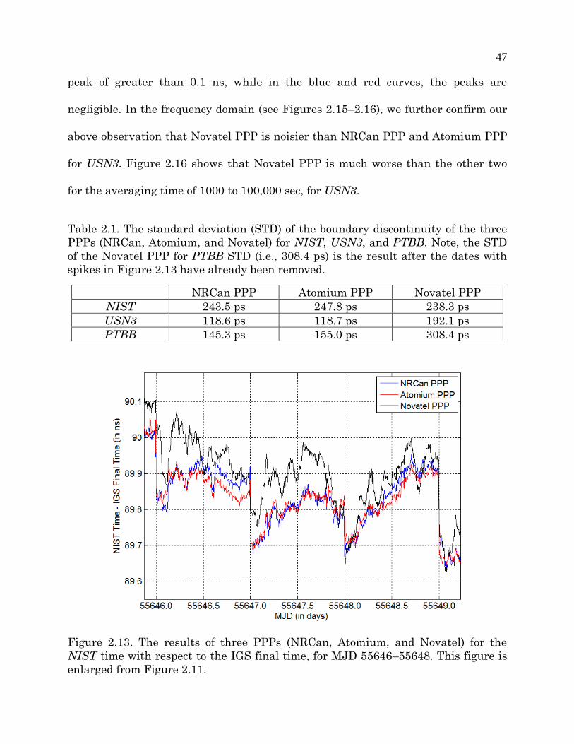
47
peak of greater than 0.1 ns, while in the blue and red curves, the peaks are
negligible. In the frequency domain (see Figures 2.15–2.16), we further confirm our
above observation that Novatel PPP is noisier than NRCan PPP and Atomium PPP
for USN3. Figure 2.16 shows that Novatel PPP is much worse than the other two
for the averaging time of 1000 to 100,000 sec, for USN3.
Table 2.1. The standard deviation (STD) of the boundary discontinuity of the three
PPPs (NRCan, Atomium, and Novatel) for NIST, USN3, and PTBB. Note, the STD
of the Novatel PPP for PTBB STD (i.e., 308.4 ps) is the result after the dates with
spikes in Figure 2.13 have already been removed.
Figure 2.13. The results of three PPPs (NRCan, Atomium, and Novatel) for the
NIST time with respect to the IGS final time, for MJD 55646–55648. This figure is
enlarged from Figure 2.11.
NRCan PPP Atomium PPP Novatel PPP
NIST 243.5 ps 247.8 ps 238.3 ps
USN3 118.6 ps 118.7 ps 192.1 ps
PTBB 145.3 ps 155.0 ps 308.4 ps

48
Figure 2.14. The results of three PPPs (NRCan, Atomium, and Novatel) for the
USN3 time with respect to the IGS final time, for MJD 55653–55655. This figure is
enlarged from Figure 2.12.
Figure 2.15. Frequency stability analysis of the three PPPs (NRCan, Atomium, and
Novatel) for NIST, for MJD 55600–55645.

49
Figure 2.16. Frequency stability analysis of the three PPPs (NRCan, Atomium, and
Novatel) for USN3, for MJD 55600–55645.
In summary, NRCan PPP and Atomium PPP exhibit a very similar
performance in terms of boundary discontinuity and frequency stability. The
Novatel PPP only works well for some stations. For other stations, the Novatel PPP
timing results could have many outliers. In addition, Novatel PPP typically provides
a bigger boundary discontinuity and worse frequency stability than the other two
PPPs. Therefore, NRCan PPP and Atomium PPP are better than Novatel PPP.

50
2.7 Appendix: Gaussian-Distribution Test of Boundary Discontinuity
In this section, we test whether the boundary discontinuity satisfies the
Gaussian distribution or not. Here, we use chi-squared (𝜒2) test to determine the
Gaussian distribution.
The basic principle of 𝜒2 test is as follows1.
First, our null hypothesis states that the distribution of the boundary
discontinuity is Gaussian. Next, the N boundary-discontinuity observations are
divided among n equally-spaced cells. In each cell, we have Oi observations. The
expected number of observations in each cell is Ei, based on the Gaussian
distribution model. Then we get the following quantity.
𝜒2 = ∑(𝑂𝑖−𝐸𝑖)
2
𝐸𝑖
𝑛𝑖=1 . (2.15)
It can be shown that for the significance level 𝛼, if
𝜒2 ≥ 𝜒𝛼2(𝑛 − 𝑚 − 1), (2.16)
where m is the number of unknown variables in the distribution model (in our case,
m=2, because only the mean and STD in the Gaussian distribution are unknown),
then we reject our null hypothesis at the significance level 𝛼.
Now let’s apply the 𝜒2 test to the Gaussian-distribution test of boundary
discontinuity. Figure 2.17 shows the boundary discontinuities of five GPS receivers
with respect to the IGS final time, instead of the IGR time. Comparing this figure
with Figure 2.7, we can see that the mean value and the STD are very close for
1 The principle of 𝜒2 test is mainly based on “Pearson’s chi-squared test” of Wikipedia. The website
link is http://en.wikipedia.org/wiki/Pearson's_chi-squared_test.

51
NIST, PTBB, and USN3. This further confirms our statement in Section 2.2 that
the boundary discontinuity behavior does not change regardless of whether the IGS
final products or the IGS rapid products are used.
Actually, we do not need to implement the algorithm of the above 𝜒2 test by
ourselves. MATLAB has already provided a function, called “chi2gof”1, to do the 𝜒2
test for a Gaussian distribution. Here, we set the significance level 𝛼 = 0.03, which
is a common setting. The corresponding command is “h = chi2gof(x, ‘Alpha’, 0.03)”. If
h is 0, then the test decision is that the data in vector x come from a Gaussian
distribution with the significance level of 0.03.
The results show that PTBB, USN3, OPMT, and USNO pass the Gaussian
distribution test. NIST is the only one that fails. Figure 2.17(a) tells us why NIST
fails. There are a few big boundary discontinuities with more than 0.5 ns jump
values. This makes the red curve wider than it should be. In the end, it makes the
blue bars not match the red curve very well. This results in that NIST fails the
Gaussian-distribution test. Without those big jumps, we can see that NIST still
observes the Gaussian distribution. Based on the above analysis, we conclude that
the boundary discontinuity is Gaussian at the significance level of 0.03. Or simply
put, the boundary discontinuity is almost Gaussian.
1 See http://www.mathworks.com/help/stats/chi2gof.html.

52
(a) (b) (c)
(d) (e)
Figure 2.17. Histograms of jumps of NIST, PTBB, USN3, OPMT, and USNO with
respect to the IGS final time. The red curve in each plot is the Gaussian-
distribution fit.

53
Chapter 3
Origin of Day Boundary Discontinuity1
3.1 Introduction: Noise and Boundary Discontinuity
As stated in Section 1.5.1, in theory, the boundary discontinuity comes from
both the code and phase noise. Here, we simulate the impact of the code and phase
noise on the boundary discontinuity.
There are basically two methods for doing the simulation. One method is to
generate ideal noise-free RINEX data. Then we add noise to the RINEX data and
see the change in the boundary discontinuity. The difficulty with this method comes
from the generation of noise-free RINEX data. Although there are some software
packages available in the world [48], we do not know their details, e.g., whether
they include the ionospheric and tropospheric delays. We may also need to revise
the PPP software package to remove some corrections in PPP.
The other method involves adding white noise to the original measured RINEX
data and studying the change in the boundary discontinuity. This method is easier
1 The results of this chapter are mainly based on [18, 47].

54
to implement. And, it can reveal the relationship between measurement noise and
boundary discontinuity quite effectively.
Here, we use the second method for our simulation. First, we keep the phase
noise at the noise level of 0.01 cycle and increase the code noise from 0.0 m to 0.5 m
(Figure 3.1). One thousand trials are done for each code noise level to get a reliable
statistical distribution. We can see from Figure 3.1 that the STD of the clock offset
at epoch 0 (that is, the very beginning epoch of the day) increases almost linearly as
the code noise increases. For a code noise of 0.3 m and a phase noise of 0.01 cycle,
which is a common noise level for the RINEX data, the STD is 85 ps, which
corresponds to the STD of the boundary discontinuity of 85 ps × 2 = 120 ps. This
value matches the statistical result of the boundary discontinuity in Section 2.4
quite well.
We can also see from Figure 3.2 that the STD of the clock offset at epoch 0
changes little for a phase noise in the range of 0.00–0.02 cycle. Because the phase
noise of the RINEX data after corrections (such as the satellite clock offsets, the
earth tide, etc.) is typically below 0.02 cycle, the phase noise has little impact on the
boundary discontinuity.

55
Figure 3.1. Relation between the clock offset at epoch 0 and the code noise
(simulation result). The phase noise is kept at the STD of 0.01 cycle.
Figure 3.2. Relation between the clock offset at epoch 0 and the phase noise
(simulation result). The pseudorange noise is kept at the STD of 0.3 m.

56
Next, we study the relation between the short-term (300 sec) stability of the
carrier-phase (CP) time transfer and the measurement noise (Figure 3.3). The time
deviation (TDEV) at an averaging time of 300 sec is used to characterize the short-
term stability. The six curves in Figure 3.3 are very close to each other, which
indicates that the code noise has little impact on the short-term stability of CP time
transfer. TDEV (300 sec) increases from 8 ps to approximately 50 ps as the phase
noise increases from 0 cycle to 0.05 cycle. This increase shows that the phase
measurement plays an important role in the short-term CP time transfer.
Figure 3.3. TDEV at 300 sec for different pseudorange noise and phase noise levels
(simulation result).
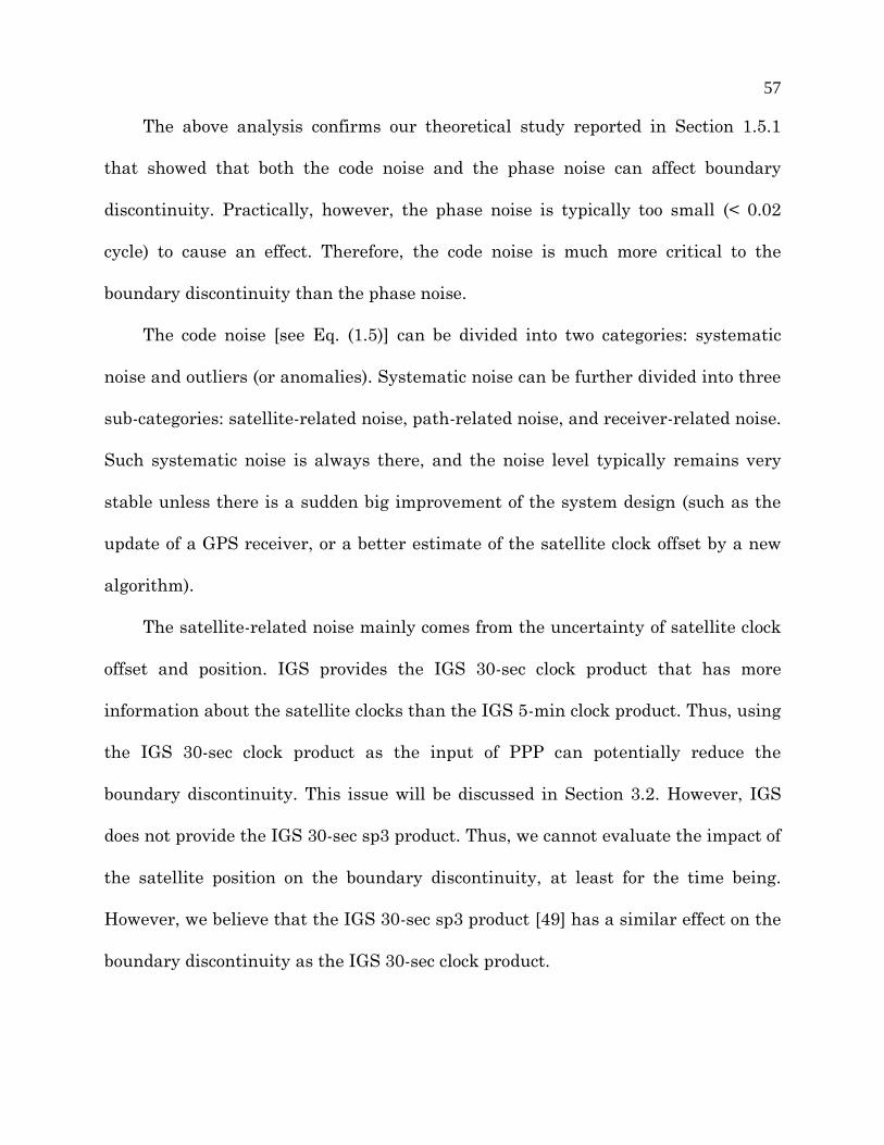
57
The above analysis confirms our theoretical study reported in Section 1.5.1
that showed that both the code noise and the phase noise can affect boundary
discontinuity. Practically, however, the phase noise is typically too small (< 0.02
cycle) to cause an effect. Therefore, the code noise is much more critical to the
boundary discontinuity than the phase noise.
The code noise [see Eq. (1.5)] can be divided into two categories: systematic
noise and outliers (or anomalies). Systematic noise can be further divided into three
sub-categories: satellite-related noise, path-related noise, and receiver-related noise.
Such systematic noise is always there, and the noise level typically remains very
stable unless there is a sudden big improvement of the system design (such as the
update of a GPS receiver, or a better estimate of the satellite clock offset by a new
algorithm).
The satellite-related noise mainly comes from the uncertainty of satellite clock
offset and position. IGS provides the IGS 30-sec clock product that has more
information about the satellite clocks than the IGS 5-min clock product. Thus, using
the IGS 30-sec clock product as the input of PPP can potentially reduce the
boundary discontinuity. This issue will be discussed in Section 3.2. However, IGS
does not provide the IGS 30-sec sp3 product. Thus, we cannot evaluate the impact of
the satellite position on the boundary discontinuity, at least for the time being.
However, we believe that the IGS 30-sec sp3 product [49] has a similar effect on the
boundary discontinuity as the IGS 30-sec clock product.

58
The path-related noise is mainly ionospheric noise and tropospheric noise. The
ionospheric noise can be cancelled out to the first order by using dual-frequency
measurements. This is what the PPP does. However, the second order of ionospheric
noise can still be as big as a few centimeters [50]. Triple-frequency measurements
can cancel out the ionospheric noise to the second order. But a triple-frequency GPS
receiver is not available in our lab. Therefore, we cannot explore the impact of high-
order ionospheric noise on boundary discontinuity in this thesis. The tropospheric
noise will be discussed in Section 3.3.
Section 3.4 will explore the receiver-related noise and propose a practical
method for reducing the impact of the receiver-related noise on the boundary
discontinuity.
An outlier or an anomaly in the RINEX data occurs quite unpredictably. The
origin of an outlier can be almost anything. For example, the GPS receiver loses the
tracking of a satellite, or the satellite-receiver line is blocked by an object, or the
reference time for the receiver is adjusted, or even a man-made error occurs. The
relationship between an outlier and the boundary discontinuity will be discussed in
Section 3.5.
Note that the results in Sections 3.2–3.5 are all based on the PPP program. As
mentioned in Section 1.5.2, the other implementation of the carrier-phase time
transfer is the network method. Section 3.6 compares the PPP method with the
network method. We’ll see that the network method is superior to the PPP method,
in terms of boundary discontinuity.

59
3.2 IGS Clock Data and Boundary Discontinuity
IGS provides the IGS 30-sec clock product that has more information about the
satellite clocks than the IGS 5-min clock product. Therefore, using the IGS 30-sec
clock product as the input of PPP could potentially reduce the boundary
discontinuity.
Figure 3.4 confirms this prediction. We run PPP for PTBB (a GPS receiver in
PTB, Germany) from Modified Julian Day (MJD) 56050 to MJD 56200 with the IGS
5-min clock product as the input [Figure 3.4(a)]. The STD of the boundary
discontinuity jump values is 163.4 ps. Then we run PPP the same but with the IGS
30-sec clock product as the input [Figure 3.4(b)]. The STD of jump values becomes
115.7 ps. The improvement over the boundary discontinuity by using the IGS 30-sec
clock product is as much as 29.2% for PTBB. Similarly, for PTBG (also in PTB,
Germany), the improvement is 22.8% [Figure 3.4(c–d)]. In addition, the mean value
of the boundary discontinuity becomes closer to 0 ps for both PTBB and PTBG.

60

61
Figure 3.4. Boundary discontinuity using the IGS 5-min clock product vs using the
IGS 30-sec clock product, for PTBB and PTBG from MJD 56050 to MJD 56200.

62
In principle, the time difference between two GPS receivers with the same
reference time at a station should be a constant [51]. In practice, the time difference
usually varies by a few nanoseconds. This variation comes from many reasons, such
as the time-transfer noise, the receiver aging, the cable extension, etc. Thus, the
comparison between two local GPS receivers can reveal whether there is any
improvement of the time-transfer result. Figure 3.5 shows the time difference
between PTBB and PTBG by using both IGS 5-min clock product and IGS 30-sec
clock product. We can clearly see that the blue curve is obviously noisier than the
red curve. This indicates that the time transfer result using the IGS 30-sec clock
product is closer to the true values than that using the IGS 5-min clock product.
Figure 3.5. Time difference between PTBB and PTBG using the IGS 5-min clock
product (blue curve) and using the IGS 30-sec clock product (red curve).

63
The improvement over the boundary discontinuity using the IGS 30-sec clock
product at several timing laboratories in the world is shown in Figure 3.6. The
improvement is typically 10–30%.
Figure 3.6. Boundary discontinuity using the IGS 5-min clock product vs using the
IGS 30-sec clock product, for several GPS receivers in the world (PTBB 56050-
56200, PTBG 56050-56200, SEPA 55927-56077, SEPB 55927-56077, SEPT 55927-
56077, USN3 56050-56200, NIST 55600-55750, AMC2 56050-56200, and OPMT
56050-56200).

64
3.3 Tropospheric Delay and Boundary Discontinuity
The tropospheric delay is separated into a predominant and well-behaved
hydrostatic (or dry) part and a much smaller and volatile wet part. Each part can be
expressed as a product of the zenith path delay (ZPD) and mapping function (M).
Therefore, the ∆𝑡𝑟𝑜𝑝𝑜 term in Eq. (1.5) can be expressed as
wetwetdrydrytropo ZPDMZPDM ** . (3.1)
The dry ZPD (i.e., 𝑍𝑃𝐷𝑑𝑟𝑦) can be modeled and considered known, but the wet
ZPD (i.e., 𝑍𝑃𝐷𝑤𝑒𝑡) must be estimated when running the PPP program [39].
There are several types of mapping functions, such as Niell mapping function
(NMF), Global mapping function (GMF), and Vienna mapping function 1 (VMF1)
[52].
NMF is expressed by Eq. (3.2):
𝑀(𝑒) =
1+𝑎
1+𝑏
1+𝑐
𝑠𝑖𝑛 𝑒+𝑎
𝑠𝑖𝑛𝑒+𝑏
𝑠𝑖𝑛𝑒+𝑐
, (3.2)
where e is the elevation of the satellite with respect to the GPS receiver, and the
parameters a, b, and c are different for the hydrostatic and wet components of the
atmosphere. Each of the parameters is a constant or a function of site latitude
(symmetric about the equator) and day of year. Thus, NMF’s temporal resolution is
about one month. VMF1 uses the output of a numerical weather analysis to provide
the information with a temporal resolution of six hours, specifically for a particular
station. Thus, VMF1 provides a quite significant improvement of the tropospheric
delay over NMF. GMF is a “back-up” mapping function or a compatible empirical

65
representation of VMF1. The parameters of a, b, c in GMF are computed based on
the average of many years of data from the numerical weather model, instead of
being estimated every 6 hours as in VMF1. Thus, GMF does not have as high
resolution as VMF1. In fact, the temporal resolution of GMF is similar to that of
NMF. Nevertheless, GMF is closer to the reality than NMF [52].
The three mapping functions of NMF, GMF, and VMF1 are shown in Figure
3.7. Clearly, VMF1 has a much higher resolution than the other two mapping
functions. NMF is away from the average and thus leads to a bias in the
tropospheric delay estimation. GMF is a good representation of VMF1 over the long
term (a few months or more).
Figure 3.7. Hydrostatic (dry) mapping function at 5 degree elevation at Fortaleza,
Brazil [52].

66
We use GMF and VMF1 in the PPP program because we want to know
whether a mapping function affects the boundary discontinuity. Thus, we run the
PPP program by using GMF and VMF1. In principle, the resolution of VMF1 (6
hours) is much higher than that of GMF (~1 month). Thus, if the tropospheric
correction in the PPP matters a lot to the boundary discontinuity, then the
boundary discontinuity should significantly decrease when we replace GMF with
VMF1. However, the boundary discontinuities we obtain using GMF and VMF1 are
almost the same (See Figures 3.8–3.9). This result indicates that the current
tropospheric correction in PPP is already good enough, and thus the noise in the
tropospheric correction has little impact on the boundary discontinuity.
3.4. Receiver-Related Noise and Boundary Discontinuity
Since we have already studied the relationship between satellite-related and
path-related noise and the boundary discontinuity in Sections 3.2–3.3, the next step
is to study the relationship between the receiver-related noise and the boundary
discontinuity.
3.4.1. Boundary Discontinuity of Receivers at the Same Station
Receivers at the same station have many common features: the same GPS
constellations, the same GPS signal transmission path, and the same reference time
for the receiver. The measurements that receivers have done differ only in their
multipaths, antennas, antenna-to-receiver cables, and receivers’ internal circuits.
Taken together, these differences make up “receiver-related noise”. The noise in the

67
reference time for a receiver should typically be negligible, in a national timing
laboratory. If the common features of receivers at the same station (i.e., the
satellite-related noise and the path-related noise) play an important role in the
boundary discontinuity, the jump values of receivers at the same station should be
highly correlated.
Figure 3.8. Histograms of jumps of PTBB for MJD 55600-55750, by using GMF.
Figure 3.9. Histograms of jumps of PTBB for MJD 55600-55750, by using VMF1.

68
However, our experimental results contradict the above assumption. SEPA,
SEPB, and SEPT are three GPS receivers at NICT (National Institute of
Information and Communications Technology, Japan). They are all Septentrio
POLARX2 receivers. The distance between each receiver is less than 5 m (See
Figure 3.10). Based on the statistics of the jump values during MJD 55600–55750,
the correlation coefficient between SEPA and SEPB is 0.471, which indicates a non-
high correlation. For SEPA and SEPT, the correlation coefficient is even less, 0.215.
The correlation coefficient between SEPB and SEPT is as small as 0.102. Thus, the
jumps of several receivers at the same station are not highly correlated, even when
the same type of receiver is used. To further confirm this, we performed a similar
comparison for PTBB and PTBG at PTB (See Figure 3.11). The correlation
coefficient is again very small, only −0.064. Based on the above analysis, we
conclude that the noise from satellites and transmission paths can contribute to
boundary discontinuity at some level, but not very much.
We also studied the correlation of jumps between two long-distance stations. It
shows that the correlation between two long-distance stations is close to 0, e.g.,
NIST & PTBB −0.011, NIST & USN3 −0.020, USN3 & PTBB 0.110. This is exactly
what we expect. After all, two long-distance stations have everything different.
They observe different sets of GPS satellites. The transmission paths are different.
The multipaths, antennas and receivers are also completely different.

69
Figure 3.10 Correlation of boundary discontinuity of SEPA, SEPB, and SEPT at
NICT, Japan.
Figure 3.11. Correlation of boundary discontinuity of PTBB and PTBG at PTB,
Germany.

70
3.4.2. Cutoff Elevation and Boundary Discontinuity
Of all types of receiver-related noise, multipath is an important factor to
study. It varies from station to station. Multipath in code measurement is usually at
the level of a few meters. Even with CP measurement smoothing, the code-
measurement bias due to multipath can still be at a several-centimeters level,
which can lead to a 100 ps clock bias. Besides, although multipath repeats every 23
h 56 min, it is different every 24 h, which may lead to different phase ambiguities
between 2 days. Thus, it is necessary for us to explore the impact of multipath on a
boundary discontinuity.
Increasing the cutoff elevation has two impacts. On the one hand, it blocks
some multipath from the low elevations which form the main part of the total
multipath. So from this point of view, we should expect a decrease of boundary
discontinuity, if multipath does affect boundary discontinuity. On the other hand,
increasing the cutoff elevation reduces the visible satellite number, which leads to
fewer observations, so it increases the uncertainty of the computed phase
ambiguity. So from this point of view, we should expect an increase of discontinuity.
However, this increase should be very small because low-elevation observations are
already given less weight than high-elevation observations. In sum, if the multipath
affects our observation seriously, we should expect a big decrease of discontinuity as
the cutoff elevation increases.
To find out the impact of multipath on the boundary discontinuity, we study
the STD of boundary discontinuity of USN3, PTBB, and SEPA at different cutoff

71
elevations during MJD 55650–55850 (Figure 3.12). We can see that the increase of
cutoff elevation gives little improvement on the boundary discontinuity. This
illustrates that the multipath, at least at USN3, PTBB, and SEPA, is not an
important factor on the magnitude of the boundary discontinuity.
Figure 3.12. Effect of cutoff elevation on boundary discontinuity.
3.4.3. Receiver Noise
Receiver-related noise includes multipath, antenna noise, antenna-to-receiver
noise, and receiver noise, as mentioned in Section 3.4.1. In this section, we focus on
the receiver noise.
In 2006, two receivers (NISA (Ashtech Z12T) and NISV (Novatel T-Sync
receiver with an OEM4 board) at NIST were connected to the same antenna [53].
We processed the RINEX data on MJD 53737 and get the measurement difference

72
(Figures 3.13–3.14) between the two receivers. The measurement difference shows
the receiver noise and the cable noise.
We can see that the code measurement has greater noise at a low satellite
elevation (Figure 3.13). Since the two receivers are connected to a common antenna,
the tropospheric noise, the ionospheric noise and the multipath noise, etc are
already cancelled by the measurement differencing. So the greater noise at low
satellite elevation in Figure 3.13 can only come from the receiver performance, e.g.,
the tracking loop performance for weak signals.
As shown in Figure 3.13, the standard deviation (STD) of the PRN04 C1 code
measurement difference is 0.53 m. The STD of L1 phase measurement difference is
0.012 cycle (Figure 3.14). If we assume that the two receivers are of the same or
similar performance, we get that the code noise due to receiver and cable is
37.02/53.0 m, and that the phase noise due to receiver and cable is 0085.02/012.0
cycle. The code and phase noise due to the receiver and cable could potentially
impact the boundary discontinuity significantly, according to the simulation result
in Section 3.1 (see Figures 3.1 –3.2).
3.4.4. Average of Receivers and Boundary Discontinuity
According to the results in Sections 3.4.1–3.4.3, we know that the receiver-
related noise is an important contributor to the boundary discontinuity. In order to
reduce the impact of the receiver-related noise on the boundary discontinuity, one
easy way is to use more GPS receivers with connections to different antennas, to
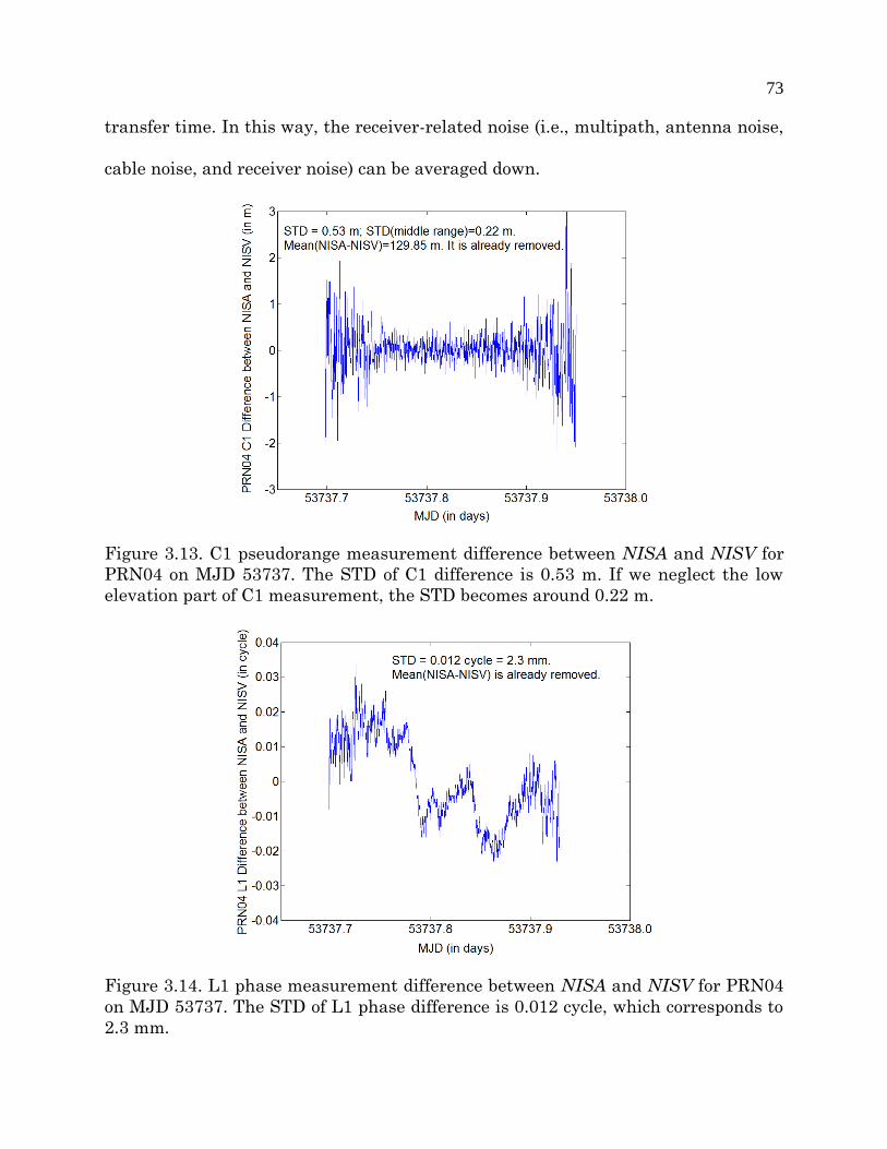
73
transfer time. In this way, the receiver-related noise (i.e., multipath, antenna noise,
cable noise, and receiver noise) can be averaged down.
Figure 3.13. C1 pseudorange measurement difference between NISA and NISV for
PRN04 on MJD 53737. The STD of C1 difference is 0.53 m. If we neglect the low
elevation part of C1 measurement, the STD becomes around 0.22 m.
Figure 3.14. L1 phase measurement difference between NISA and NISV for PRN04
on MJD 53737. The STD of L1 phase difference is 0.012 cycle, which corresponds to
2.3 mm.

74
For NISA at NIST, the STD of the boundary discontinuity jump values is 167.2
ps for MJD 56230–56380. For NISX at NIST, the STD is 215.0 ps for the same
period. If we do averaging over the two receivers, the STD becomes 124.0 ps, which
indicates an improvement of 25.8%. We also do averaging for SEPA and SEPB at
NICT (Japan) for MJD 55927–56077, and PTBB and PTBG at PTB for MJD 56050–
56200. The improvements by averaging two receivers at the same station are 13.7%
and 15.9%, respectively (Figure 3.15).
Figure 3.15. Average of receivers and boundary discontinuity for NIST (NISA and
NISX), NICT (SEPA and SEPB) and PTB (PTBB and PTBG). The magenta bar is
the average of two receivers at a station.
The average of receivers also helps reduce the short-term (< 30 min) noise by
10–20% (Figure 3.16). On the other hand, this also indicates that the conventional

75
CP time transfer cannot observe the short-term (<30 min) clock noise very well
because the actual clock noise cannot be averaged down by using two GPS receivers.
Figure 3.16. Improvement of the average of receivers on the short-term time
transfer frequency stability. For the averaging time of 5 min and 10 min, the
average of the receivers gives an improvement of 10–20%.
3.5. Bad Points and Boundary Discontinuity
We find that a bad data point (or a data anomaly) in the RINEX file can affect
not only the time at that specific epoch, but also the whole time at all epochs and
thus the boundary discontinuity, especially when the bad point happens at the
beginning or at the end of the data-arc.
For example, we run PPP for NIST with the input of the RINEX data-arc from
19:40:00 to 19:39:30 of the next day (e.g., from 19:40:00 of MJD 55647 to 19:39:30 of
MJD 55648). The result is shown by the blue curve in Figure 3.17 (blue, red, and

76
black curves are very close except for the second data-arc in Figure 3.17.). We can
see that the boundary discontinuity is obviously below 500 ps. However, if we shift
the RINEX data-arc by 5 min (that is, we run PPP for the data-arc from 19:45:00 to
19:44:30 of the next day (red curve in Figure 12)), the boundary discontinuity is now
greater than 3 ns. This huge boundary discontinuity comes from the bad point
happening at 19:40:00 of MJD 55649. If we remove the two bad PRNs (PRN14 and
PRN31) measurements at this epoch, then the huge boundary discontinuity
disappears (magenta curve, which is very close to the green curve and the black
curve). The black curve shows the case of data-arc of 19:50:00 to 19:49:30 of the next
day. The boundary discontinuity of the black curve is again smaller than 500 ps.
This example shows that if a bad data point happens at the end of the data-arc, we
could have a huge boundary discontinuity.

77
Figure 3.17. Illustration of the impact of a bad data point on the boundary
discontinuity. The blue curve is the result for the data-arc of 19:40:00 to 19:39:30 of
the next day. The red curve is the result for the data-arc of 19:45:00 to 19:44:30 of
the next day. The magenta curve is the corrected result of the red curve on the
second data-arc after the bad data are removed. The black curve is the result for the
data-arc of 19:50:00 to 19:49:30 of the next day.
Bad points can not only seriously affect the boundary discontinuity as
mentioned above, but also damage the whole time transfer result (such as the slope)
of a single data-arc. Figure 3.18 shows this problem. We have already detected that
there are a few bad points between 15:00:00 and 16:00:00 of MJD 55647 for USN3
(at USNO, USA). This period (MJD 55647.625–55647.667) is marked by the big

78
black rectangle in Figure 3.18. At the time around MJD 55646.5, all curves are
approximately parallel. That indicates the slope is almost the same no matter how
we shift the RINEX data, which is what we expect. The difference between two
adjacent curves is around 0.2 ns. The slight difference from 0.2 ns comes from
different boundary discontinuities due to shifted data-arcs. The same situation
occurs at around MJD 55648.5. However, the slopes of all curves are not the same
around MJD 55647.5 because of the bad points happening from 15:00:00 to 16:00:00
on this day. For example, at MJD 55647.60, the bottom black curve reads 7.685 ns.
The bottom red curve almost reads the same value as the bottom black curve. At
MJD 55647.75, the bottom red curve reads 7.817 ns. However, the bottom black
curve reads 7.607 ns. The slope difference between the two curves during MJD
55647.60–55647.75 is as big as 1.4 ns / day. Remember that we use exactly the same
RINEX data and run PPP with exactly the same settings. The only difference is that
we shift the RINEX data by a few hours. In principle, the slope difference of two
curves should be very close to 0. Because of the existence of bad points, we have
totally different time transfer results. These different results make us hard to tell
which one is correct or whether both of them are wrong. This example demonstrates
how seriously a few bad points can damage the whole time transfer result of a
single data-arc.

79
Figure 3.18. Illustration of how bad points damage the time transfer result of the
same data-arc. The curves are shifted along the y-axis by multiples of 0.2 ns for
better comparison. Each curve begins at a different start point (e.g., the magenta
curve begins at 15:15:00; the bottom green curve begins at 00:00:00).
3.6. PPP Method and Network Method on Boundary Discontinuity
As mentioned in Section 1.5.2, there are two implementation methods of GPS
carrier-phase time transfer: the network method and the PPP method. The PPP
method is easier to implement and faster than the network method. However, the
result of the PPP method may not be as good as that of the network method. This

80
occurs because it does not solve all equations from all stations in the world together.
Thus, there could potentially have a small timing and positioning bias in the result
of the PPP method. Such a bias may lead to a bigger boundary discontinuity. Thus,
we want to compare the two methods in terms of the boundary discontinuity.
Actually, the IGS clock file has already provided the results of the network
method for many ground stations. Figure 3.19 shows the comparison between the
PPP method and the network method. We can see that the mean jump value is
closer to 0 in the network method than the PPP method. Furthermore, the STD is
typically more than 20 ps in the network method than in the PPP method. This
means that the network method is superior to the PPP method in terms of boundary
discontinuity. Any improvement in the algorithm for implementing the GPS carrier-
phase time transfer can give a smaller discontinuity, even though the noise in
physical measurement is still the same.
3.7. Summary
In this chapter, we find that the code noise is the major contributor to the
boundary discontinuity. The code noise can be divided into three categories:
satellite-related noise, path-related noise, and receiver-related noise. We find that
by using the IGS 30-sec clock product, the boundary discontinuity can be lowered by
10–30%. The tropospheric path noise seems have little impact on the boundary
discontinuity. The boundary discontinuity can be further lowered by 10–20% if a
few GPS receivers at the same station are averaged. The anomaly in the RINEX

81
data can also sometimes lead to a big boundary discontinuity and an incorrect slope
in the time transfer. The comparison between the PPP method and the network
method indicates that the network method provides a smaller boundary
discontinuity.
(a)
(b)
Figure 3.19. Effect of algorithms of fixing ambiguity on boundary discontinuity. (a)
shows the absolute mean of discontinuity of both the PPP method and the network
method for five stations. (b) shows the STD of discontinuity.

82
Chapter 4
Eliminating Day Boundary Discontinuity: RINEX-Shift algorithm1
4.1 RINEX-Shift Algorithm
As we discussed in the last chapter, the day boundary discontinuity comes from
any type of code noise. Although the code noise can be reduced by some methods, it
is impossible to get it down to zero. Thus, the boundary discontinuity cannot be
removed by reducing the code noise. However, this does not mean that there is no
way to eliminate the boundary discontinuity. In fact, a few algorithms have been
proposed to eliminate the boundary discontinuity to achieve continuous GPS CP
time transfer [43, 46–47, 54–57]. One promising algorithm among them is the
RINEX-Shift (RS) algorithm [47, 54].
Figure 4.1 shows how the RS algorithm works. The conventional PPP runs first
forward (from the beginning of the data-arc to the end of the data-arc) and then
backward (from the end of the data-arc to the beginning of the data-arc) in order to
converge the solutions [38]. The backward results (one point per 5 min) form the
final PPP output. As shown in Figure 4.1(a), the blue dots and the red dot together
1 The results of this chapter are mainly based on [47, 54].

83
are the backward results of PPP. Since the phase ambiguity is almost always away
from the true value due to the code noise, the solution of one data-arc almost always
has a jump from the solution of the next data-arc. This jump is the boundary
discontinuity.
A good way to “eliminate” the boundary discontinuity is to make the length of
the data-arc to be 5 min so that every point has its own estimation of phase
ambiguity. Now the boundary discontinuity is actually transformed from a long
data-arc (≥ 1 day) to a short data-arc (e.g., 5 min). The boundary discontinuity of a
short data-arc cannot be noticed because it is combined with the short-term (e.g., 5
min) noise. In this way, we no longer have the boundary discontinuity, and the
carrier-phase (CP) time transfer can be used for a long-term (e.g., 20 days) time
comparison without the impact of the day boundary discontinuity.
Another thing to consider is that the use of a short data-arc can hardly give a
converged estimate of the zenith path delay of the troposphere, etc. Thus, the short-
term noise can be huge because of a large uncertainty in the phase ambiguity. A
good way to tackle this issue is to run PPP for a long data-arc and extract the result
at the first epoch point of the backward process [the red dot in Figure 4.1(a)]. Then
we shift the RINEX data by another time step (e.g., 5 min, or 10 min, or even
greater) and executes PPP, and then extracts the result at the new first epoch again
[Figure 4.1(b)]. So on and so forth [Figure 4.1(c)-(d)]. The results at all the first
epochs [the red dots in Figure 4.1(a)-(d)] form the final result. In this way, we can

84
not only eliminate the boundary discontinuity, but also have small short-term noise.
We call this process the RINEX-Shift (RS) algorithm.
Figure 4.1. Illustration of the RINEX-Shift algorithm.
To test this algorithm, we choose the “NIST” receiver at NIST and the “PTBB”
receiver at PTB (Physikalisch-Technische Bundesanstalt, Germany). We set the
data-arc of the RS algorithm to 10 days and the time step to 10 min. Then we run
the RS algorithm and get the time difference between the NIST time and the PTBB
time during Modified Julian Date (MJD) 56389–56409 (red curve in Figure 4.2). The
black curve in Figure 4.2 is the result of the conventional PPP with a 1-day data-
arc, as a reference. As we can see, there are day boundary discontinuities in the
black curve. These discontinuities disappear in the red curve. This indicates that
the RS algorithm eliminates day boundary discontinuities successfully.
The modified total deviation (MTD) is used to characterize the frequency
stability. Figure 4.3 shows the MTD of the black and red curves in Figure 4.2. The
RS algorithm reduces the time-transfer noise significantly, especially at the range

85
of 4 hours to 4 days. The MTD of the RS result (red curve in Figure 4.3) becomes flat
for an averaging time of greater than 1 day, which indicates that we have already
seen the UTC(k) clock noise after 1 day.
Figure 4.2. Time comparison between NIST and PTBB during MJD 56389–56409 by
NRCan PPP (black curve) and the RINEX-Shift (RS) algorithm (red curve). The
curves are shifted to overlay each other for better comparison.

86
Figure 4.3. MTD of the time difference between NIST and PTBB for MJD 56389–
56409, using NRCan PPP (black curve) and the RINEX-Shift (RS) algorithm (red
curve).
4.2 Problem with RINEX-Shift Algorithm
The RS algorithm showed excellent performance in terms of eliminating the
boundary discontinuity as shown in Section 4.1. However, this excellent
performance is only the case when all of the GPS data are good. Although most
timing laboratories have installed state-of-the-art GPS receivers and antennas, it is
still inevitable that a GPS receiver malfunctions (e.g., losing track of GPS

87
satellites), or the satellite-receiver line is blocked by an object, or the reference time
for the receiver is adjusted, or even a man-made error occurs. All these problems
lead to GPS data anomalies. We find that if there are a few epochs of data
anomalies, the result of the RS algorithm deviates from the true value (Figures 4.4–
4.5).
In Figure 4.4, we compare the time difference between PTBB [a GPS receiver
in PTB, Germany] and the International GNSS Service (IGS) final time. The black
curve is the result of the NRCan PPP software package. We can see that there is an
obvious day boundary discontinuity between MJD 56610 and MJD 56611. Since the
standard deviation of the boundary discontinuity of PTBB is only 138.5 ps [18], we
can hardly distinguish other small day boundary discontinuities at the scale of
Figure 4.4. The red curve is the result computed by the RS algorithm. It eliminates
the boundary discontinuity very well (e.g., there is no jump between MJD 56610
and MJD 56611).

88
Figure 4.4. Comparison of NRCan PPP (black curve) and the RINEX-Shift
algorithm (red curve) at anomalies at PTB. (b) is enlarged from (a).
However, the RINEX data of PTBB show that there are three time periods of
missing GPS data during MJD 56609.0–56616.0. The first one occurs between
(a)
(b)
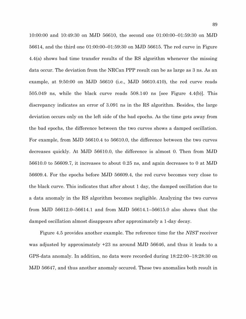
89
10:00:00 and 10:49:30 on MJD 56610, the second one 01:00:00–01:59:30 on MJD
56614, and the third one 01:00:00–01:59:30 on MJD 56615. The red curve in Figure
4.4(a) shows bad time transfer results of the RS algorithm whenever the missing
data occur. The deviation from the NRCan PPP result can be as large as 3 ns. As an
example, at 9:50:00 on MJD 56610 (i.e., MJD 56610.410), the red curve reads
505.049 ns, while the black curve reads 508.140 ns [see Figure 4.4(b)]. This
discrepancy indicates an error of 3.091 ns in the RS algorithm. Besides, the large
deviation occurs only on the left side of the bad epochs. As the time gets away from
the bad epochs, the difference between the two curves shows a damped oscillation.
For example, from MJD 56610.4 to 56610.0, the difference between the two curves
decreases quickly. At MJD 56610.0, the difference is almost 0. Then from MJD
56610.0 to 56609.7, it increases to about 0.25 ns, and again decreases to 0 at MJD
56609.4. For the epochs before MJD 56609.4, the red curve becomes very close to
the black curve. This indicates that after about 1 day, the damped oscillation due to
a data anomaly in the RS algorithm becomes negligible. Analyzing the two curves
from MJD 56612.0–56614.1 and from MJD 56614.1–56615.0 also shows that the
damped oscillation almost disappears after approximately a 1-day decay.
Figure 4.5 provides another example. The reference time for the NIST receiver
was adjusted by approximately +23 ns around MJD 56646, and thus it leads to a
GPS-data anomaly. In addition, no data were recorded during 18:22:00–18:28:30 on
MJD 56647, and thus another anomaly occured. These two anomalies both result in
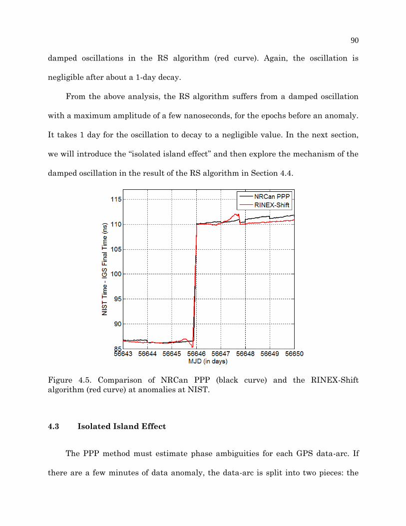
90
damped oscillations in the RS algorithm (red curve). Again, the oscillation is
negligible after about a 1-day decay.
From the above analysis, the RS algorithm suffers from a damped oscillation
with a maximum amplitude of a few nanoseconds, for the epochs before an anomaly.
It takes 1 day for the oscillation to decay to a negligible value. In the next section,
we will introduce the “isolated island effect” and then explore the mechanism of the
damped oscillation in the result of the RS algorithm in Section 4.4.
Figure 4.5. Comparison of NRCan PPP (black curve) and the RINEX-Shift
algorithm (red curve) at anomalies at NIST.
4.3 Isolated Island Effect
The PPP method must estimate phase ambiguities for each GPS data-arc. If
there are a few minutes of data anomaly, the data-arc is split into two pieces: the

91
first sub-data-arc and the second sub-data-arc. PPP typically treats the second sub-
data-arc (i.e., the data after the anomaly) as a new data-arc and thus re-estimates
phase ambiguities that are usually different from the estimations for the first sub-
data-arc. Because of different phase-ambiguity estimations for the first and second
sub-data-arcs, we have a boundary discontinuity at the anomaly (Figure 4.6).
The blue curve in Figure 4.6 shows the PPP result for the original RINEX data
of PTBB on MJD 56489. It is continuous because there is no anomaly. However, if
we delete 10 minutes of RINEX data, e.g., 13:00:30–13:10:00, then the PPP result
has a boundary discontinuity of 1.07 ns at 13:00:00 (red curve). If the 10-min
missing-data window occurs at other epochs (grey, orange, black, green, and
magenta curves), we still have a boundary discontinuity, although the jump value
varies. This illustrates that an anomaly leads to a boundary discontinuity. Note
that the slopes of all curves are more or less the same. Thus, an anomaly is not too
bad, if only frequency transfer, instead of time transfer, is our main concern.
However, the above analysis is based on the premise that an anomaly occurs in
the middle range of a data-arc. If an anomaly occurs at the beginning or the end of a
data-arc, the behavior of the PPP result becomes quite different.

92
Figure 4.6. Anomaly in the middle range of the data-arc and boundary
discontinuity. The blue curve is the original PPP result for PTBB on MJD 56489.
All other curves are the PPP results with 10-min missing data.
Figure 4.7 shows the PPP results when the 10-min missing-data window is
close to the beginning of a data-arc. The blue curve is the PPP result of the original
RINEX data, for reference. If the missing-data window occurs at 00:00:30–00:10:00
(that means that 00:00:00 is the only epoch of valid data before the anomaly since
the GPS receivers record RINEX data every 30 s.), the time transfer error can be as
large as 1.7 ns (solid red curve at 00:00:00). This is because the phase ambiguity
cannot be solved for if only one epoch of measurements is provided [19, Chapter 6].
This makes the phase measurements useless. Thus, the time solution at 00:00:00
can only be determined by the code measurements, which are much noisier than the
phase measurements. As the missing-data window shifts away from the data-arc

93
edge (e.g., the dashed red curve), we have a longer period of valid data (in this case,
it is 30 min) between the edge and the anomaly. Therefore, we are now getting a
better estimation of the phase ambiguities. However, this estimation is still not
good enough. Reference [38] tells us that the PPP program requires at least 1 hour
of data to converge to an accurate estimation of phase ambiguities. 30 min is still
not sufficient for PPP to converge to a reasonable result, which makes the dashed
red curve still quite noisy during the first sub-data-arc. When the missing-data
window occurs more than 1 hour away from the edge (e.g., the dashed green curve
in Figure 4.7), the PPP result for the first sub-data-arc becomes smooth.
Figure 4.7. Anomaly at the beginning of the data-arc and boundary discontinuity.
The blue curve is the original PPP result for PTBB on MJD 56489. All other curves
are the PPP results with 10-min of missing data.

94
From the above analysis, we know that an anomaly in the middle range of a
data-arc results in a boundary discontinuity, but the time-transfer slope is almost
unchanged; an anomaly at the edge of a data-arc (less than 1 hour from the edge)
results in a completely damaged PPP result between the anomaly and the edge. We
call this phenomenon the “isolated island effect.”
4.4 Mechanism of Damped Oscillation in the RINEX-Shift Algorithm
In the RS algorithm, we run PPP for a data-arc of 10 days and extract the PPP
result at the first epoch (here, we define the PPP result at the first epoch as
“PPP_FE”). If the anomaly is more than 10 days away from the first epoch, it does
not affect the result of the RS algorithm. However, as we shift the RINEX data step
by step, the new data-arc starts to cover the anomaly. The anomaly first shows at
the end of the data-arc, and thus the length of the first sub-data-arc is 10 days
(here, we define the length of the first sub-data-arc, i.e., the time difference between
the anomaly and the first epoch, as deltaT). Then the RINEX data continue shifting
and deltaT changes from 10 days to 0. At the same time, all PPP_FEs are extracted
to form the RS solution. In the end, the data-arc goes over the anomaly (i.e., deltaT
becomes negative), and thus the anomaly no longer affects the result of the RS
algorithm. From the above, we can see that the RS solution after the anomaly is not
affected by the anomaly, but the RS solution before the anomaly is determined by
the relationship between PPP_FE and deltaT. Thus, we next study this
relationship.

95
Actually, we have already had the “PPP_FE–deltaT” relationship if we
interpret Figures 4.6–4.7 in a different perspective. For the grey curve in Figure 4.6,
the length of the first sub-data-arc “deltaT” is 2 hours, and the PPP result at the
first epoch (i.e., 00:00:00) is 508.926 ns, which is +0.624 ns away from the original
PPP result (blue curve in Figure 4.6) at 00:00:00. Thus, we have (deltaT, PPP_FE) =
(2.008 hours, 508.926 ns). Similarly, for the orange curve in Figure 4.6, we have
(deltaT, PPP_FE) = (5.008 hours, 508.794 ns). So on and so forth. This gives a series
of (deltaT, PPP_FE) pairs. The red curve in Figure 4.8 shows the result (note, it
uses some curves not shown in Figures 4.6–4.7). The original PPP result at 00:00:00
is given for reference (blue curve).
Figure 4.8. PPP_FE–deltaT graph. The PPP_FE–deltaT relationship determines the
RS solution before the anomaly.

96
We can see that Figure 4.8 and Figure 4.4(b) have many common features,
demonstrating that the “PPP_FE–deltaT” relationship does determine the result of
the RS algorithm. First, in Figure 4.8, we can clearly see that PPP_FE (red curve) is
approximately 1.7 ns away from the original PPP result (blue curve) when deltaT is
close to 0. This indicates that the error in the RS algorithm can be as large as
several nanoseconds when the anomaly is very close to the first epoch. This matches
our results in Figure 4.4(b). Second, when deltaT increases from 0 to 40 min,
PPP_FE decays toward the original PPP result very quickly (Figure 4.8). This decay
is very similar to the behavior of the RS solution during MJD 56610.375–56610.403
[red curve in Figure 4.4(b)]. Third, for the range of 2 hours to a few hours, Figure
4.8 shows that PPP_FE decreases slowly and steadily toward the original PPP
result, which is again quite similar to the RS solution for the time range of
56610.05–56610.33 in Figure 4.4(b). Finally, when deltaT is more than 20 hours,
PPP_FE becomes smaller than the original PPP result (Figure 4.8). But the
absolute maximum difference between PPP_FE and the original PPP result is only
about 0.059 ns, which is much smaller than if deltaT is in the range of 2 hours to a
few hours. This indicates a damped oscillation in PPP_FE. Again, the behavior of
PPP_FE at deltaT > 20 hours matches the damped oscillation behavior in the result
of the RINEX-Shift algorithm (Figure 4.4(b)).
The above analysis shows that the PPP_FE–deltaT relationship does
determine the RS result. Because the PPP_FE–deltaT relationship is derived from
the isolated island effect, we conclude that it is the isolated island effect that leads

97
to the damped oscillation behavior in the RS algorithm. In addition, the scope of the
isolated island effect is approximately 1 day. Once a sub-data-arc is longer than 1
day, the impact of the isolated island effect on the RS algorithm is negligible.
4.5 Revised RINEX-Shift Algorithm
Based on the discussion in Sections 4.2–4.4, we know that if an anomaly is less
than 1 day away from the edge of a data-arc (i.e., deltaT < 1 day), the time-transfer
result of the RS algorithm in between is incorrect, because of the isolated island
effect. If deltaT > 1 day, the result in between becomes reasonable. Thus we must
avoid the situation when the anomaly is less than 1 day away from the data-arc
edge. If we can achieve this, we can solve the damped oscillation problem in the RS
algorithm. One good way is to extract the PPP result at the middle epoch of the
data-arc, instead of the first epoch of the data-arc as in the RS algorithm. We call
this the “revised RINEX-Shift (RRS)” algorithm. The following example explains
how this algorithm works.
In Figure 4.4, there is an anomaly occurring at 01:00:00 on MJD 56614 (i.e.,
56614.042). When we run PPP for the data-arc of MJD 56604.044–56614.044, the
anomaly starts to affect the time-transfer result. We know that the result of the
second sub-data-arc (i.e., 56614.043–56614.044) is completely damaged because the
length of this sub-data-arc is too short for PPP to converge. However, the result of
the first sub-data-arc (i.e., 56604.044–56614.041) is still good because the length of
this sub-data-arc is greater than 1 day, and the isolated island effect is negligible. If

98
the RRS algorithm is applied, the PPP result at the middle epoch (i.e., 56609.044) is
extracted. Since the middle epoch is within the first sub-data-arc, the PPP result at
this epoch is good. As we continue shifting the data-arc until 56609.040–56619.040,
the first sub-data-arc changes from 56604.044–56614.041 to 56609.040–56614.041.
When the data-arc is 56609.040–56619.040, the length of the first sub-data-arc is
5.001 days, which is still long enough to make the isolated island effect negligible.
Thus, the result at the middle epoch (i.e., 56614.040) extracted by the RRS
algorithm is still good. Next, the data-arc shifts to 56609.043–56619.043. Now the
PPP result at 56614.043 is extracted. This epoch is within the second sub-data-arc
(i.e., 56614.042–56619.043). Since the second sub-data-arc is again longer than 1
day, the PPP result at 56614.043 is still good.
From the above example, we can see that once we extract the middle epoch of
the data-arc, the sub-data-arc where the middle epoch lies is always longer than 5
days, which is long enough to eliminate the impact of the isolated island effect.
Thus, the RRS algorithm should provide reasonable results at all epochs. We report
tests of its performance in the next section.
4.6 Performance of Revised RINEX-Shift Algorithm
In this section, we first test the performance of the RRS algorithm when there
is an anomaly in the RINEX data. Figures 4.9–4.10 show the results of the RRS
algorithm for the same periods as Figures 4.4–4.5. Similar to NRCan PPP (black
curve) and the RS algorithm (red curve), the revised RINEX-Shift algorithm (blue

99
curve) has a boundary discontinuity at the anomaly (e.g., MJD 56610.417). This
discontinuity occurs because the epochs before and after the anomaly belong to two
different sub-data-arcs, and thus different phase ambiguities are estimated. Like
the RS algorithm, the RRS algorithm eliminates the day boundary discontinuities
successfully. Most importantly, as compared to the RS algorithm, there is no
damped oscillation problem in the RRS algorithm.
Figure 4.9. Comparison of NRCan PPP (black curve), RS algorithm (red curve) and
RRS algorithm (blue curve) at anomalies at PTB.
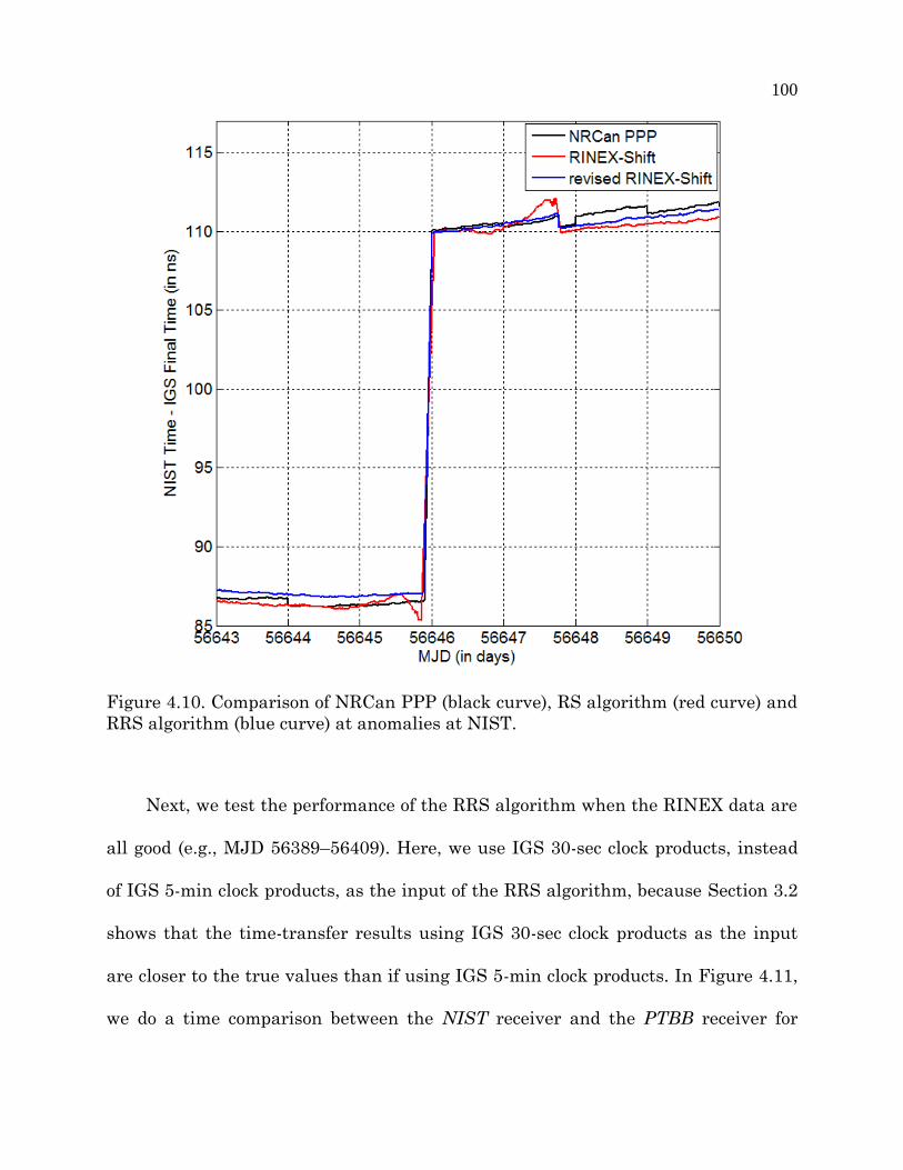
100
Figure 4.10. Comparison of NRCan PPP (black curve), RS algorithm (red curve) and
RRS algorithm (blue curve) at anomalies at NIST.
Next, we test the performance of the RRS algorithm when the RINEX data are
all good (e.g., MJD 56389–56409). Here, we use IGS 30-sec clock products, instead
of IGS 5-min clock products, as the input of the RRS algorithm, because Section 3.2
shows that the time-transfer results using IGS 30-sec clock products as the input
are closer to the true values than if using IGS 5-min clock products. In Figure 4.11,
we do a time comparison between the NIST receiver and the PTBB receiver for

101
MJD 56389–56409 by NRCan PPP (black curve), RS algorithm (red curve), and RRS
algorithm (blue curve). We can see that both RS and RRS provide continuous time-
transfer results. The modified total deviation (MTD) is used to characterize the
frequency stability of the three time-transfer methods (Figure 4.12). Obviously, the
RRS algorithm provides the best frequency stability. It reduces the time-transfer
noise of the RS algorithm by 10–55%. The most significant improvement of the RRS
algorithm over the RS algorithm occurs at the averaging time of 1–4 days. For an
averaging time of 1.75 days, the frequency stability of the RRS algorithm is only 8.6
× 10−16, which makes it the best GPS time-transfer result. In addition, the MTD of
the RRS algorithm increases for an averaging time of greater than 1.75 days, which
indicates that we have already seen the clock noise after 1.75 days.
Figure 4.11. Time comparison between NIST and PTBB during MJD 56389–56409
by NRCan PPP (black curve), RS algorithm (red curve), and RRS algorithm (blue
curve). The curves are shifted to overlay each other for better comparison.

102
Figure 4.12. MTD of the time difference between NIST and PTBB for MJD 56389–
56409 using NRCan PPP (black curve), RS algorithm (red curve), and RRS
algorithm (blue curve).
As stated in [56], the smoothest time-transfer solution is not necessarily the
most accurate solution. The above analysis only shows that the RRS algorithm does
provide the smoothest solution. Next, we need to test the accuracy of the RRS
algorithm. This can be done by comparing two receivers at the same station,
because the reference clock noise is cancelled out, and only the time transfer noise
remains. Figure 4.13 shows the time difference between the NIST receiver and the
NIS2 receiver at NIST determined by using different time-transfer methods [47].

103
We can clearly see that NRCan PPP solutions (blue, black, and orange curves) are
quite artificial. The time difference between the two common-reference-clock
receivers is not continuous. The RS algorithm (red curve) provides a continuous
time transfer. However, compared to the RRS result, the RS result seems more
artificial. For example, at MJD 56400.0, the red curve decreases very quickly. In
contrast, there is almost no decrease in the NRCan PPP solutions (black and orange
curves) and the RRS solution at this epoch. For another example, there is a peak
with an amplitude of about 0.6 ns during MJD 56411–56416 in the red curve. In
contrast, the peak is tiny in the RRS solution (green curve), which matches the
NRCan PPP 30-day data-arc solution (orange curve). Both the NRCan PPP result
and the RRS result for MJD 56440–56460 are smooth. In contrast, the RS solution
for this period is quite noisy. All these features lead to the conclusion that the RRS
algorithm provides time-transfer results closer to the true values than does the RS
algorithm.
To further verify the above conclusion, we do another test. We run the RRS
algorithm, together with RS, NRCan PPP, and TWSTFT (Two-Way Satellite Time
and Frequency Transfer), for NIST and PTB for MJD 56375–56476 (Figure 4.14).
Note, for the red and green curves, two receivers at NIST (NIST and NIS2) and two
receivers at PTB (PTBB and PTBG) are used and averaged, respectively, because
this can potentially provide a better time transfer result (see Section 3.4.4). We can
see that TWSTFT (blue curve in Figure 4.14) has a diurnal oscillation that makes it
a poor choice for short-term time transfer. The NRCan PPP with a 1-day data-arc

104
typically has a boundary discontinuity each day, which degrades the long-term time
transfer result. Besides, the slope of each day also does not match the trend of
TWSTFT well. For example, the black curve goes up on MJD 56378, while the blue
curve goes down. For another example, the black curve is flat on MJD 56401, while
the blue curve tends to go down. This inconsistency between TWSTFT and the
NRCan PPP indicates that the NRCan PPP could have a wrong slope and thus an
incorrect time comparison result. The NRCan PPP with a 10-day data-arc (magenta
curve) and the NRCan PPP with a 30-day data-arc (orange curve) also do not match
TWSTFT very well, though they are better than the NRCan PPP with a 1-day data-
arc. We can see that the magenta curve drifts away from the blue curve. Then there
is a boundary discontinuity that makes it match the blue curve again (e.g., the
boundary at MJD 56385.0, 56405.0, 56425.0, and 56455.0, etc). Thus, the slope and
the boundary discontinuity compensate each other. Since the boundary
discontinuity should not appear in nature, we can say that the NRCan PPP result
has an incorrect slope. Some people propose that we can use a longer data-arc (e.g.,
35 days or 40 days) in order to avoid the appearance of the boundary discontinuity
in the time range we are interested [44]. This method can still hardly avoid the
incorrect slope. Thus, a time comparison using the conventional NRCan PPP with a
super long data-arc could still introduce some man-made error. The “RINEX-Shift”
result and the “revised RINEX-Shift” result are very close to each other (red curve
and green curve in Figure 4.14). Both of them match TWSTFT very well. The
boundary discontinuity in RS/RRS disappears, and the slope also matches the trend

105
of TWSTFT quite well. We should mention that we cannot distinguish RRS from RS
in the time domain as shown in Figure 4.14. However, in the frequency domain
(next paragraph), we will see the difference between RRS and RS.
To characterize how well all GPS carrier-phase time transfer results in Figure
4.14 match TWSTFT mathematically, we study the MTD of the difference between
TWSTFT and each GPS carrier-phase time transfer (see Figure 4.15). Figure 4.15
clearly shows that the RRS result matches TWSTFT best. An obvious improvement
of the RRS algorithm over the RS algorithm occurs at the averaging time of 2–15
days. In addition, the slope of the green curve during 1–15 days is approximately
−1. This indicates that the flicker phase-modulation noise [15] dominates in the
RRS time transfer during 1–15 days. Note that the green curve in Figure 4.15 sets
the upper limit of the RRS time transfer noise (e.g., the RRS time-transfer noise is
less than 4×10⁻¹⁶ for an averaging time of 4.25 days).

106
Figure 4.13. Time difference between NIST and NIS2 for MJD 56375–56476, using
different PPP time transfer methods [NRCan PPP with 1-day data-arc (blue curve),
NRCan PPP with 10-day data-arc (black curve), NRCan PPP with 30-day data-arc
(orange curve), RS algorithm (red curve), and RRS algorithm (green curve)].

107
Figure 4.14. Time difference between UTC(NIST) and UTC(PTB) for MJD 56375–56476 by using TWSTFT (blue
curve), NRCan PPP with a 1-day data-arc (black curve), NRCan PPP with a 10-day data-arc (magenta curve),
NRCan PPP with a 30-day data-arc (orange curve), RS algorithm (red curve), and RRS algorithm (green curve). The
curves are shifted by some constants for a better comparison.

108
Figure 4.15. MTD of the double difference between TWSTFT and different GPS
carrier-phase time-transfer methods [NRCan PPP with 1-day data-arc (blue curve),
NRCan PPP with 10-day data-arc (black curve), NRCan PPP with 30-day data-arc
(orange curve), RS algorithm (red curve), and RRS algorithm (green curve)], for
MJD 56375–56476.
To provide the time transfer noise of the RS and RRS algorithms, we merge
Figure 4.12 and Figure 4.15 together. In this way, we have the characteristic of the

109
RS and RRS time transfer noise for both short term (< 1 day) and long term (> 1
day) (see Figure 4.16).
The details about how we merge Figure 4.12 and 4.15 into Figure 4.16 are
worth discussing. First, for a short term, the time difference between two long-
distance stations (Figure 4.12) has noise from both clock and time transfer (note
that the short-term UTC(k) clock noise is typically smaller than the time transfer
noise). Thus, Figure 4.12 sets the upper limit for time transfer noise. To be
conservative, we simply set Figure 4.16 the same as Figure 4.12 for the short term.
The actual short-term time-transfer noise should be smaller than what Figure 4.16
shows. Second, for a long term, we assume that TWSTFT and carrier-phase time
transfer have a comparable noise level (In fact, TWSTFT should be noisier than
carrier-phase in the long term. To be conservative, we assume they are the same.).
Thus, the long-term time transfer noise in Figure 4.16 comes from the result in
Figure 4.15 divided by √2.
From Figure 4.16, we know that the RRS algorithm provides the smallest time-
transfer noise. For example, the fractional frequency stability is 3 × 10⁻¹⁵ for an
averaging time of ~0.5 days; the stability is 1 × 10⁻¹⁵ for an averaging time of ~1
day; and the stability is 1 × 10⁻¹⁶ for an averaging time of ~10 days.
As a whole, the RRS algorithm successfully removes the RS algorithm’s
damped-oscillation problem that occurs before the anomaly. More importantly, it
matches TWSTFT best and reduces the time-transfer noise of the RS algorithm by
10–55%. This makes the RRS algorithm the best GPS time-transfer method.

110
Figure 4.16. Frequency stability of different carrier-phase time-transfer techniques
[NRCan PPP with a 1-day data-arc (blue curve), RINEX-Shift algorithm (red curve),
and revised RINEX-Shift algorithm (green curve)]. The purple dotted line is the
frequency stability of a single Cesium fountain clock [36]. The red dotted line is the
frequency stability of two Cesium fountain clocks compared to each other.
4.7 Fountain Comparisons
Now we want to apply the new time-transfer technique (i.e., RS/RRS
algorithm) to Cesium (Cs) fountain clock comparisons.

111
A single Cs fountain-clock noise (purple dotted line in Figure 4.16) was
evaluated in [36] (also see Figure 2.2 in Section 2.1). If we want to compare two
long-distance fountain clocks, the total fountain-clock noise (red dotted line in
Figure 4.16) should be √2 of that of a single fountain clock, if we assume the two
fountain clocks have the same performance.
From Figure 4.16, we can see that the clock noise is a major contributor after
about half a day if the RS/RRS time-transfer technique is applied. In contrast, if the
conventional NRCan PPP (or carrier-phase) time-transfer technique is used, the
clock behavior only starts to be observed after 5 days! Clearly, the RS/RRS time
transfer technique pushes the long-distance clock-observation threshold from 5 days
to 0.5 days.
As an example, we compare the NIST F1 Cs fountain with the Paris
Observatory (OP, France) FO2 Cs fountain during MJD 56497.7–56533.6 by
TWSTFT, NRCan PPP (1-day data-arc), and the RS algorithm (Figure 4.17). The
TWSTFT shows that there is a long-term oscillation between two fountain clocks.
The period is approximately 20 days. However, the obvious diurnal problem (i.e.,
about 0.6 ns peak-to-peak) in TWSTFT degrades its short-term resolution. Without
solving the diurnal problem in TWSTFT, TWSTFT is not very good for precise time
comparison, such as a Cs Fountain-clock comparison. The conventional NRCan PPP
(1-day data arc) is accepted by many national laboratories for precision time
transfer. Even though NRCan PPP provides a good short-term stability (< 6 hours),
it is even worse than TWSTFT in the long term (blue curve). For example, it can

112
hardly resolve the 20-day oscillation behavior between the two fountain clocks
because of the day boundary discontinuity. In contrast, the RS algorithm (red curve)
solves the day boundary discontinuity perfectly (note that two GPS receivers, NIST
and NISA, are used at NIST in the RS algorithm.). It resolves the 20-day oscillation
behavior very well. Besides, it can also see the short-term (~0.5 day) clock behavior
quite well. For example, at around MJD 56520.0, there is a sudden decrease in the
red curve. Checking with the trend of the blue curve at around MJD 56520.0, we
can also see a decrease. This confirms that this decrease comes from the clock
behavior. This also indicates that the RS/RRS time transfer is able to resolve short-
term (~0.5 day) clock behavior.
In terms of frequency stability, we get Figure 4.18 based on Figure 4.17 (note,
the bump occurring at an averaging time of 10 days comes from the 20-day
oscillation behavior in fountain clocks). Clearly, the RS/RRS time transfer has the
smallest noise in the fountain comparison. TWSTFT is worse than the RS/RRS time
transfer in both the short term (< 1 day) and the long term (> 1 day). NRCan PPP is
comparable to the RS/RRS time transfer in the super-short term (< 3 hours).
However, it is inferior to the RS/RRS time transfer for an averaging time of longer
than 6 hours. When we look at the total fountain clock noise (red dotted line), we
can see that the clock noise becomes a major contributor after ~12 hours in the
RS/RRS time transfer. In contrast, in TWSTFT and NRCan PPP, the time-transfer
noise dominates until approximately 6 days. This result matches our prediction at

113
the beginning of this section that the RS/RRS time-transfer technique pushes the
long-distance clock-observation time threshold from ~5 days to ~0.5 days.
From the above analysis, the RS/RRS algorithm provides an obviously better
time-transfer result than both TWSTFT and the conventional carrier-phase time-
transfer (or PPP) technique. This makes the RS/RRS algorithm good for observing
the short-term (~0.5 day) behavior of a long-distance Cesium fountain clock.
4.8 Summary
This chapter proposed the RINEX-Shift (RS) algorithm to solve the day-
boundary-discontinuity problem in the carrier-phase time transfer. This algorithm
showed a performance superior to the conventional carrier-phase time transfer. The
revised RS (RRS) algorithm was designed to improve the performance of the RS
algorithm at data anomalies. In addition, the RRS algorithm also provided 10–55%
better short-term and long-term stability than the RS algorithm. Most importantly,
the RS/RRS result matched TWSTFT better than the conventional carrier-phase
time-transfer techniques. All these features indicate that the RS/RRS algorithm is
the best carrier-phase time-transfer technique for the time being. Finally, we
explored the applications of the RS/RRS algorithm. It showed that the RS/RRS
algorithm allowed us to observe long-distance Cs fountain-clock behavior after 0.5
days. In contrast, TWSTFT and the conventional carrier-phase time transfer
required at least 5 days.

114
Figure 4.17. Fountain Comparison between NIST F1 Cs fountain and OP FO2 Cs fountain for MJD 56497.7–56533.6
by using TWSTFT (black curve), NRCan PPP with 1-day data-arc (blue curve), and the RS algorithm (red curve).

115
Figure 4.18. Total deviation of time difference between NIST F1 Cs fountain and OP
FO2 Cs fountain for MJD 56497.7–56533.6, using TWSTFT (black curve), NRCan
PPP with 1-day data-arc (blue curve), and the RS algorithm (red curve).

116
Chapter 5
Boundary Discontinuity Due To GPS Measurements Anomaly1
5.1 Introduction
As stated in Section 1.6, there are two categories of boundary discontinuity.
The first category of boundary discontinuity is “data-batch boundary discontinuity”,
which has been discussed in Chapters 2–4. The second category of boundary
discontinuity is “boundary discontinuity due to GPS measurements anomaly” (for
short, anomaly-BD). This chapter focuses on the second category of boundary
discontinuity.
Within one data batch, there may be some missing data or bad data caused by
many reasons. For example, an extreme ionospheric activity can lead to a change of
tens of nanoseconds of path delay [59]. The satellite-receiver line may be blocked by
some objects. The reference time for the receiver may also be adjusted. Even the
receiver may function incorrectly [60]. Although people have proposed some
strategies of better monitoring ionosphere [61] or re-designing a GPS receiver, the
1 The results of this chapter are mainly based on [58].

117
problem of missing/bad data is almost inevitable. When there are missing/bad data,
the PPP software usually re-estimates the phase ambiguity after the anomaly.
Thus, there can be a discontinuity at the anomaly.
As an example, we compare the time difference between NISA (a GPS receiver
at NIST) and the IGS final time on Modified Julian Date (MJD) 56325 by using
PPP. The original PPP result is shown by the blue curve in Figure 5.1. The blue
curve is continuous because of no data anomaly. However, if we delete 10 min of
RINEX data (note that RINEX data provide the code and phase measurements of a
GPS receiver), the PPP result (black curve in Figure 5.1) has a discontinuity at the
time of the missing data. In this specific case, the discontinuity is as big as ~250 ps.
Figure 5.1. Illustration of the “boundary discontinuity due to GPS measurements
anomaly”. The blue curve is the PPP result with the original RINEX file as the
input. The black curve is the PPP result with the RINEX file lacking the data
between 8:00:00–8:09:30 as the input. Note, NISA is a GPS receiver at NIST.

118
From the above, we know that a few minutes of GPS measurement anomaly is
enough to lead to a discontinuity of a few hundred picoseconds in the GPS carrier-
phase time transfer. This anomaly-BD is typically at the same level of the day
boundary discontinuity. With the revised RINEX-Shift (RRS) algorithm, we are able
to eliminate the day boundary discontinuity very well. However, this algorithm can
do nothing with the anomaly-BD. Thus, we want to find a strategy to deal with this
category of boundary discontinuity (i.e., anomaly-BD).
5.2 Curve Fitting for GPS Code and Phase Measurements
A straightforward strategy for dealing with the anomaly-BD is to do curve
fitting for the anomaly. We first extract the code and phase measurements for each
satellite from the RINEX file. Then we detect the anomaly. If there is an anomaly,
then we use polynomial regression (typically the 9th or 10th order of the polynomial)
to fit the good data both before and after the anomaly. Then the fitted result during
the time range of the anomaly is used to replace the missing/bad measurements. In
the end, we save the fitted code and phase measurements to the RINEX file. Now,
when we run PPP with the revised RINEX file as the input, PPP does not need to
re-estimate the phase ambiguities at the anomaly since the anomaly has already
been “repaired”. Thus, we should have a continuous time-transfer result at the
anomaly. Of course, the time-transfer result during the time range of the anomaly
should finally be disregarded, because the RINEX data at the anomaly is “made” by
the polynomial regression.

119
An important reminder here is that this strategy only works very well for
national laboratories that have near-perfect reference clocks, or GPS receivers with
very good rubidium or cesium clocks as their references. This strategy does not work
well for the RINEX data recorded by the GPS receiver without a precise reference
clock. For example, a quartz oscillator can drift by more than 100 ns in an hour. If
the GPS receiver only has a quartz oscillator as the reference clock, the instability
of the quartz oscillator can lead to an uncertainty of the curve-fitted RINEX data
being hundreds of nanoseconds or even more. Thus, PPP still needs to re-estimate
the phase ambiguities. Therefore, the boundary discontinuity at the anomaly is still
there and cannot be removed by the curve-fitting strategy.
5.3 Verification of Curve-Fitting Strategy
To verify the curve-fitting strategy in Section 5.2, we first run carrier-phase
time transfer for the original good GPS measurements data recorded by the NISA
receiver at NIST (from MJD 56325.000 to MJD 56325.999). There is no
discontinuity because of no anomaly (see the blue curve in Figure 5.2). Then we
delete 20 min of measurements data (6:00:00–6:19:30) and run the carrier-phase
time transfer (see the black curve in Figure 5.2). The time difference between
56325.250 and 56325.264 is as big as 260 ps, which indicates a discontinuity.

120
Figure 5.2. Boundary discontinuity due to 20 min of GPS missing data (black
curve). The blue curve is the time transfer with all good data, as a reference.
Now, let’s implement the curve-fitting strategy. We do curve fitting for the 20
min of missing data for each satellite by using the good data during 5:30:00–5:59:30
and 6:20:00–6:49:30 (i.e., half an hour before the anomaly and half an hour after the
anomaly). Figure 5.3(a) shows the fitted result of phase measurements for PRN01,
as an example. Figure 5.3(b) shows the difference (or residual) between the original
data and the fitted data during 5:30:00–6:49:30. Clearly, during the time range of
missing data (6:00:00–6:19:30), the difference between the original data and the
fitted data is less than 0.1 cycle (i.e., less than 1.9 cm). The rms of the difference is
121
0.03 cycle (i.e., 0.57 cm). Figure 5.4 is similar to Figure 5.3, but is for code
measurements. The rms of the difference between the original data and the fitted
data is 0.67 m.
Admittedly, PRN01, as an IIF-block satellite, has a rubidium clock with a
small short-term (< 3 hours) noise. Thus, the satellite clock noise has little impact
on the curve fitting result. Because of this, we have a very small rms of phase
measurements, as shown in Figure 5.3(b). However, for the PRNs from the old
satellite blocks, such as Block IIA and Block IIR, the short-term (< 3 hours) clock
noise is larger. Thus, the rms of phase measurements (Figure 5.5) is typically
greater than PRN01. However, this does not mean that the rms is very large.
Figure 5.5 actually shows that the rms is below 0.3 cycle (i.e., 5.7 cm), which is still
an acceptable curve-fitting result. The rms of code measurements for other PRNs
(Figure 5.6) is similar to PRN01, i.e., ~0.7 m, because the satellite clock noise is only
a small part of the total code noise.
From the above discussion, we can see that the curve fitting for code and phase
measurements works very well. Statistically, the rms of the residuals after curve
fitting for code measurements is typically less than 0.8 m. And, the rms of the
residuals for phase measurements is typically less than 5.7 cm. Thus, with the
fitted code and phase measurements, we can potentially “make” the data good.
Because the data are “good” after applying the curve-fitting strategy, we can now
avoid the re-estimation of phase ambiguities at the anomaly in the PPP processing,
and thus eliminates the anomaly-BD.

122
Figure 5.3. Curve fitting of the phase measurements for PRN01. Missing data
occurs during 6:00:00–6:19:30. The blue curve in (a) is the phase measurements for
PRN01 during 5:30:00–5:59:30 and 6:20:00–6:49:30. The red curve in (a) is the 9th
order of polynomial fitting. (b) is the phase-measurements difference (or residual)
between the original data and the fitted data during 5:30:00–6:49:30.
(a)
(b)

123
Figure 5.4. Curve fitting of the code measurements for PRN01. Missing data occurs
during 6:00:00–6:19:30. The blue curve in (a) is the code measurements for PRN01
during 5:30:00–5:59:30 and 6:20:00–6:49:30. The red curve in (a) is the 9th order of
polynomial fitting. (b) is the code-measurements difference (or residual) between the
original data and the fitted data during 5:30:00–6:49:30.
(b)
(a)

124
Figure 5.5 The phase-measurements difference (or residual) between the original
data and the fitted data during 5:30:00–6:49:30, for PRN19. It is similar to Figure
5.3(b).

125
Figure 5.6. The code-measurements difference (or residual) between the original
data and the fitted data during 5:30:00–6:49:30, for PRN19. It is similar to Figure
5.4(b).
To test the conjecture that the curve-fitting strategy can eliminate the
anomaly-BD, we replace the 20-min missing data in the RINEX file with the fitted
data and then run PPP for the revised RINEX file. The result is shown by the red
curve in Figure 5.7. Clearly, the discontinuity just disappears. This demonstrates
that the curve-fitting strategy successfully solves the discontinuity problem in the
black curve. We have also conducted the same procedures as the above for the
anomaly occurring at other times, such as 7:00:00–7:19:30, 12:00:00–12:19:30. All of

126
them show a very similar continuous time-transfer result as shown by the red curve
in Figure 5.7. This further confirms our conclusion that the curve-fitting strategy
works very well for the boundary-discontinuity problem at a data anomaly.
Figure 5.7. Curve-fitting strategy for eliminating the anomaly-BD (red curve). The
blue and red curves are the same as Figure 5.2. They are included in this figure for
comparison.
5.4 Summary and Outlook
In this chapter, we discussed the anomaly-BD, and proposed the polynomial
curve-fitting strategy to solve this problem. Tests showed that this strategy worked
quite well for up to 20 min of measurements anomaly.

127
Admittedly, there is still a lot of work to do in order to completely solve the
problem of anomaly-BD. For example, what we discussed in this chapter mainly
focused on the situation where we have good data before and after the anomaly.
However, in practice, we may have a big step after the anomaly, due to either a
cycle slip or a time step in the reference clock of a GPS receiver. Even at national
laboratories, a time step of tens of nanoseconds in the reference clock occurs from
time to time (typically, a few times a year). This time step may come from changing
the current time scale to a backup time scale, or from updating the time-
distribution system, or even from replacing the time-reference cable for the GPS
receiver. The cycle slips can typically be corrected during the pre-processing of PPP.
However, the time steps in the reference clock are not so easy to deal with. For the
time steps in the reference clock, the carrier-phase time transfer must re-estimate
the phase ambiguities. Thus, the observed time step is a combination of the actual
time step and a boundary discontinuity introduced by the time step. If we can find a
method to eliminate the boundary discontinuity due to this type of anomaly, we can
better estimate the actual time step in the reference clock.
As we know, satellite clock noise can be as big as a few cm for an averaging
time of 5 min. In Section 5.3, we do curving fitting for the code and phase
measurements. But these measurements include the satellite clock noise. Thus, the
residual after curve fitting contains the satellite clock noise. This makes the curve
fitting imperfect. A better strategy for curve fitting would be to apply the precise
satellite clock offsets (i.e., IGS clk data) to the code and phase measurements first,

128
and then do polynomial curve fitting next. In this way, the residual after curve
fitting will become smaller. I have done some tests on this new strategy. The
residual of L1 phase measurements reduces from ~0.8 cycle (peak-to-peak) to 0.06
cycle (peak-to-peak), for most GPS satellites. We expect that this new strategy may
push the current allowed data-anomaly window of 20 min further to approximately
1 hour.

129
Chapter 6
Summary
In this thesis, we report studies of the day boundary discontinuity (day-BD)
problem in GPS carrier phase time transfer (GPSCPTT).
In terms of statistics, we find that the day-BD has a near-Gaussian
distribution. Different stations have different means and standard deviations (STD)
of day-BD. Besides, as the data-arc length increases (e.g., from 1 day to 4 days),
both mean and STD of day-BD increases. In particular, the mean increases linearly.
This makes the 35-day data-arc GPSCPTT done by the International Bureau of
Weights and Measures (BIPM) problematic.
The origin of day-BD comes from the re-estimation of phase ambiguities for the
next day. We find code noise, instead of phase noise, mainly leads to day-BD. We
find that the boundary discontinuity can be reduced by 10–30% using IGS 30-sec
clock products, instead of IGS 5-min clock products. The tropospheric path noise
seems have little impact on the boundary discontinuity. The boundary discontinuity
can be further lowered by 10–20% if a few GPS receivers at the same station are
averaged. The anomaly in the RINEX data can also sometimes lead to a large
130
boundary discontinuity and an incorrect slope in the time transfer. The comparison
between the PPP method and the network method indicates that the network
method provides a smaller boundary discontinuity.
To eliminate day-BD, we have designed the RINEX-Shift (RS) algorithm and
the revised RINEX-Shift (RRS) algorithm. Both of them provide continuous
GPSCPTT results. However, the RS algorithm has a damped-oscillation problem
when GPS data have anomalies. We proposed the RRS algorithm to solve this
problem. RS/RRS matches two-way satellite time/frequency transfer (TWSTFT)
much better than the conventional GPSCPTT. The RS/RRS time transfer noise is
typically 1.4 × 10⁻¹⁴ for an averaging time of 1 hr, 2.5 × 10⁻¹⁵ for 0.5 day, 1.0 × 10⁻¹⁵
for 1 day, 3.0 × 10⁻¹⁶ for 4 days, and 7.5 × 10⁻¹⁷ for 20 days. We are able to observe
the high-precision Cesium fountain clock behavior after 0.5 day using RS/RRS time
transfer, instead of ~5 days using the conventional GPSCPTT. This makes RS/RRS
the best GPS time-transfer technique.
In addition to day-BD, we also have a boundary discontinuity at the data
anomaly (anomaly-BD) because of re-estimation of phase ambiguities. We proposed
a simple polynomial curve-fitting strategy to repair the data anomaly. The curve-
fitted GPS phase data are typically less than 6 cm from the actual GPS phase data.
Tests show that this strategy works for at least a 20-min data anomaly. Thus, we
have successfully eliminated the anomaly-BD.
In a summary, with the effort of studying and eliminating the BD problem, we
have achieved continuous GPS carrier-phase time transfer.

131
Bibliography
[1] S. R. Jefferts, T. P. Heavner, and E. A. Donley, “Cesium primary frequency
references,” Jpn. J. Appl. Phys., vol. 43, no. 5B, pp. 2803–2807, 2004.
[2] W. H. Oskay, S. A. Diddams, E. A. Donley, T. M. Fortier, T. P. Heavner, L.
Hollberg, W. M. Itano, S. R. Jefferts, M. J. Delaney, K. Kim, F. Levi, T. E.
Parker, and J. C. Bergquist, “Single-atom optical clock with high accuracy,”
Phys. Rev. Lett. 97, 020801, 2006.
[3] B. J. Bloom, T. L. Nicholson, J. R. Williams, S. L. Campbell, M. Bishof, X.
Zhang, W. Zhang, S. L. Bromley, and J. Ye, “An optical lattice clock with
accuracy and stability at the 10−18 level,” Nature, vol. 506, pp. 71–75, 2014.
[4] N. Hinkley, J. A. Sherman, N. B. Phillips, M. Schioppo, N. D. Lemke, K.
Beloy, M. Pizzocaro, C. W. Oates, and A. D. Ludlow, “An atomic clock with
10−18 instability,” Science, vol. 341, pp. 1215–1218, 2013.
[5] T. Rosenband, D. B. Hume, P. O. Schmidt, C. W. Chou, A. Brusch, L. Lorini,
W. H. Oskay, R. E. Drullinger, T. M. Fortier, J. E. Stalnaker, S. A. Diddams,
W. C. Swann, N. R. Newbury, W. M. Itano, D. J. Wineland, and J. C
Bergquist, “Frequency ratio of Al+ and Hg+ single-ion optical clocks;
metrology at the 17th decimal place,” Science, vol. 319, pp. 1808–1812, 2008.
[6] F. L. Walls, and D. W. Allan, “Measurements of frequency stability,”
Proceedings of the IEEE, vol. 74, pp. 162–168, 1986.
[7] S. A. Diddams, D. J. Jones, J. Ye, S. T. Cundiff, J. L. Hall, J. K. Ranka, R. S.
Windeler, R. Holzwarth, T. Udem, and T. W. Hänsch, “Direct link between
microwave and optical frequencies with a 300 THz Femtosecond laser comb,”
Phys. Rev. Lett. 84, 5102, 2000.

132
[8] S. Romisch, S. R. Jefferts, and T. E. Parker, “Towards an all-digital time
scale,” Proc. IEEE Frequency Control Symposium Joint with the EFTF, pp.
685–689, 2011.
[9] Z. Li, W. Zhou, H. Zhou, X. Zhang, and J. Zhao, “The optimization of super-
high resolution frequency measurement techniques based on phase
quantization regularities between any frequencies,” Rev. Sci. Instrum. 84,
025106, 2013.
[10] W. Lewandowski, and C. Thomas, “GPS time transfer,” Proceedings of the
IEEE, vol. 79, pp. 991–1000, 1991.
[11] J. R. Ray, “IGS/BIPM time transfer pilot project,” GPS Solutions, vol. 2, pp.
37–40, 1999.
[12] W. Lewandowski, and J. Azoubib, “Time transfer and TAI,” Proc. IEEE/EIA
IFCS 2000 Conference, pp. 586–597, 2000.
[13] S. Bregni, “Synchronization of digital telecommunications networks,”
Chichester, UK: John Wiley & Sons, 2002.
[14] T. Adam, et al, “Measurement of the neutrino velocity with the OPERA
detector in the CNGS beam,” arXiv:1109.4897v4, 2012.
[15] W. J. Riley, “Handbook of frequency stability analysis,” NIST Special
Publication 1065, 2008.
[16] D. W. Allan, N. Ashby, and C. C. Hodge, “The Science of Timekeeping,”
Hewlett Packard Application Note 1289, 1997.
[17] E. D. Kaplan, “Understanding GPS: principles and applications,” Artech
House, Boston, MA, 1996.
[18] J. Yao and J. Levine, “GPS carrier-phase time transfer boundary
discontinuity investigation,” Proc. 44th Annual Precise Time and Time
Interval Systems and Applications (PTTI) Meeting, pp. 317–326, 2012.
[19] B. Hofmann-Wellenhof, H. Lichtenegger, E. Wasle, “GNSS global navigation
satellite systems: GPS, GLONASS, Galileo and more,” Springer, Berlin, 2008.
[20] J. Levine, “A review of time and frequency transfer methods,” Metrologia, 45,
pp. S162–S174, 2008.
[21] T. E. Parker, and D. Matsakis, “Time and frequency dissemination: advances
in GPS transfer techniques,” GPS World, November, pp. 32–38, 2004.

133
[22] D. W. Hanson, “Fundamentals of two-way time transfer by satellite”, Proc.
43rd Annual Frequency Control Symposium, pp. 174–178, 1989.
[23] V. Zhang, T. E. Parker, J. Achkar, A. Bauch, L. Lorini, D. Matsakis, D.
Piester, and D. G. Rovera, “Two-way satellite time and frequency transfer
using 1 MChip/s codes,” Proc. 41st PTTI Meeting, pp. 371–382, 2009.
[24] D. W. Allan and M. A. Weiss, “Accurate time and frequency transfer during
common-view of a GPS satellite,” Proc. 34th Ann. Freq. Control Symposium,
1980.
[25] D. W. Allan, M. A. Weiss, and N. Ashby, “Around-the-world relativistic
sagnac experiment,” Science, vol. 228, pp. 69–70, 1985.
[26] G. Petit and Z. Jiang, “GPS All in View time transfer for TAI computation,”
Metrologia, 45, pp. 35–45, 2008.
[27] K. M. Larson, and J. Levine, “Carrier-phase time transfer,” IEEE Trans.
Ultrason., Ferroelect., Freq. Contr., vol. 46, pp. 1001–1012, 1999.
[28] C. Hackman, J. Levine, T. E. Parker, D. Piester, and J. Becker, “A
straightforward frequency-estimation technique for GPS carrier-phase time
transfer,” IEEE Trans. Ultrason., Ferroelect., Freq. Contr., vol. 53, pp. 1570–
1583, 2006.
[29] P. Defraigne and C. Bruyninx, “On the link between GPS pseudorange noise
and day-boundary discontinuities in geodetic time transfer solutions,” GPS
Solutions, vol. 11, pp. 239–249, 2007.
[30] K. Senior, E. Powers, and D. Matsakis, “Attenuating day-boundary
discontinuities in GPS carrier-phase time transfer,” Proc. 31st PTTI Meeting,
pp. 481–490, 1999.
[31] N. Guyennon, G. Cerretto, P. Tavella, and F. Lahaye, “Further
characterization of the time transfer capabilities of precise point positioning
(PPP): the sliding batch procedure,” IEEE Trans. Ultrason., Ferroelect., Freq.
Contr., vol. 56, no. 8, pp. 1634–1641, 2009.
[32] M. Weiss, J. Yao, and J. Li, “In search of a new primary GPS receiver for
NIST,” Proc. 44th PTTI Meeting, pp. 179–186, 2012.
[33] R. Dach, G. Beutler, U. Hugentobler, S. Schaer, T. Schildknecht, T. Springer,
G. Dudle, and L. Prost, “Time transfer using GPS carrier phase: error
propagation and results,” J. Geodesy, vol. 77, pp. 1–14, 2003.

134
[34] P. Misra, and P. Enge, “Global positioning system: signals, measurements,
and performance (revised 2nd edition),” Ganga-Jamuna Press, Lincoln, MA,
2012.
[35] J. Zumberge, M. B. Hefflin, D. C. Jefferson, M. M. Watkins, F. H. Webb,
“Precise point positioning for the efficient and robust analysis of GPS data
from large networks,” J. Geophys. Res., vol. 102, pp. 5005–5017, 1997.
[36] S. R. Jefferts, T. P. Heavner, T. E. Parker, and J. H. Shirley, “NIST Cesium
fountains – current status and future prospects,” Proc. of SPIE Vol. 6673,
667309, 2007.
[37] C. Hackman, J. Levine, and T. E. Parker, “A long-term comparison of GPS
carrier-phase frequency transfer and two-way satellite time/frequency
transfer,” Proc. 38th PTTI Meeting, pp. 485–498, 2006.
[38] J. Kouba and P. Heroux, “Precise point positioning using IGS orbit and clock
products,” GPS Solutions, vol. 5, pp. 12–28, 2001.
[39] J. Kouba, “A guide to using International GNSS Service (IGS) products,” IGS
Central Bureau, Pasadena (available at ftp://ftp.igs.org/pub/resource/pubs/
UsingIGSProductsVer21.pdf).
[40] http://igscb.jpl.nasa.gov/igscb/data/format/sp3_docu.txt.
[41] http://igscb.jpl.nasa.gov/igscb/data/format/rinex_clock300.txt
[42] http://igscb.jpl.nasa.gov/igscb/data/format/rinex210.txt
[43] C. Bruyninx, P. Defraigne, “Frequency transfer using GPS code and phases:
short- and long-term stability,” Proc. 31st PTTI Meeting, pp. 471–480, 1999.
[44] G. Petit, “The TAIPPP pilot experiment,” Proc. EFTF-IFCS 2009 Joint
Conference, pp. 116–119, 2009.
[45] Q. Baire, C. Bruyninx, P. Defraigne, and J. Legrand, “Precise point
positioning with Atomium using IGS orbit and clock products: first results,”
Bulletin of Geodesy and Geomatics, vol. 69, n. 2-3, pp. 396–404, 2010.
[46] P. Defraigne, C. Bruyninx, and N. Guyennon, “PPP and phase-only GPS time
and frequency transfer,” Proc. IEEE Frequency Control Symposium Joint
with the 21st EFTF, pp. 904–908, 2007.
[47] J. Yao and J. Levine, “A new algorithm to eliminate GPS carrier-phase time
transfer boundary discontinuity,” Proc. 45th PTTI Meeting, pp. 292–303,
2013.

135
[48] E. Mohino, M. Gende, C. Brunini, and M. Heraiz, “SiGOG: simulated GPS
observation generator,” GPS Solutions, vol. 9, pp. 250–254, 2005.
[49] J. Griffiths, and J. R. Ray, “On the precision and accuracy of IGS orbits,” J.
Geod., vol. 83, pp. 277–287, 2009.
[50] S. Datta-Barua, T. Walter, J. Blanch, and P. Enge, “Bounding higher-order
ionosphere errors for the dual-frequency GPS user,” Radio Science, vol. 43,
RS5010, 2008.
[51] C. Hackman and J. Levine, “New frequency comparisons using GPS carrier-
phase time transfer,” Proc. IEEE IFCS 2003 Conference, pp. 258–265, 2003.
[52] J. Boehm, A. Niell, P. Tregoning, and H. Schuh, “Global mapping function
(GMF): a new empirical mapping function based on numerical weather model
data,” Geophys. Res. Lett., vol. 33, L07304, 2006.
[53] M. Hottovy and M. Weiss, “Differential delay between two geodetic GPS
receivers for L1 and L2 code and carrier signals,” Proc. IEEE IFCS 2008
Conference, pp. 496–500, 2008.
[54] J. Yao, and J. Levine, “An improvement of RINEX-Shift algorithm for
continuous GPS carrier-phase time transfer,” Proc. 27th ION GNSS+ 2014
Conference, pp. 1253–1260, 2014.
[55] R. Dach, T. Schildknecht, T. Springer, G. Dudle, and L. Prost, “Continuous
time transfer using GPS carrier phase,” IEEE Trans. Ultrason., Ferroelect.,
Freq. Contr., vol. 49, no. 11, pp. 1480–1490, 2002.
[56] R. Dach, T. Schildknecht, U. Hugentobler, L.-G. Bernier, and G. Dudle,
“Continuous geodetic time transfer analysis method,” IEEE Trans. Ultrason.,
Ferroelect., Freq. Contr., vol. 53, no. 7, pp. 1250–1259, 2006.
[57] J. Delporte, F. Mercier, D. Laurichesse, and O. Galy, “GPS Carrier-Phase
Time Transfer Using Single-Difference Integer Ambiguity
Resolution,” International Journal of Navigation and Observation, vol. 2008,
Article ID 273785, 7 pages, 2008.
[58] J. Yao, and J. Levine, “GPS measurements anomaly and continuous GPS
carrier-phase time transfer,” To be published in Proc. 46th PTTI Meeting,
2014.
[59] V. Zhang, “GPS time and frequency transfer activities at NIST,” 54th Civil
GPS Service Interface Committee (CGSIC) Meeting, 2014.

136
[60] D. Matsakis, “Report from the U. S. Naval Observatory,” 53rd Civil GPS
Service Interface Committee (CGSIC) Meeting, 2013.
[61] J. Jing, S. K. Khanafseh, F. C. Chan, S. Langel, and B. Pervan, “Detecting
ionospheric gradients for GBAS using a null space monitor,” Proc. IEEE-ION
PLANS, pp. 1125–1133, 2012.