Continued Fractions, Euclidean Algorithm and Lehmer’s Algorithm

Applied Symbolic ComputationCS 567

Jeremy Johnson

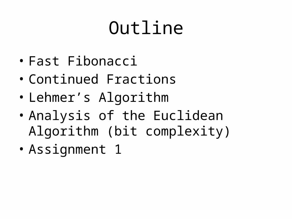
Outline

• Fast Fibonacci• Continued Fractions• Lehmer’s Algorithm• Analysis of the Euclidean Algorithm (bit

complexity)• Assignment 1

Euclidean Algorithm

g = gcd(a,b) a1 = a; a2 = b; while (a2 0) a3 = a1 mod a2; a1 = a2; a2 = a3; } return a1;

Remainder Sequence

a1 = a, a2 = ba1 = q3 a2 + a3, 0 a3 < a2

ai = qi ai+1 + ai+2, 0 ai+2 < ai+1

al= ql al+1

gcd(a,b) = al+1

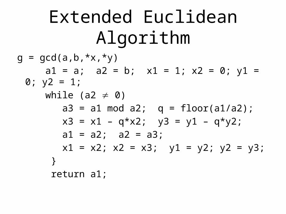
Extended Euclidean Algorithm

g = gcd(a,b,*x,*y) a1 = a; a2 = b; x1 = 1; x2 = 0; y1 = 0; y2 = 1; while (a2 0) a3 = a1 mod a2; q = floor(a1/a2); x3 = x1 – q*x2; y3 = y1 – q*y2; a1 = a2; a2 = a3; x1 = x2; x2 = x3; y1 = y2; y2 = y3; } return a1;

Lehmer’s Algorithm

u = 27182818, v = 10000000

u’ v’ q’ u’’ v’’ q’’2718 1001 2 2719 1000 21001 716 1 1000 719 1 716 285 2 719 281 2 285 146 1 281 157 1 146 139 1 157 124 1 139 7 19 124 33 3 u’/v’ < u/v < u’’/v’’

Maximum Number of Divisions

Theorem. Let a b 0 and n = number of divisions required by the Euclidean algorithm to compute gcd(a,b). Then n < 2lg(a).

Maximum Number of Divisions

Theorem. The smallest pair of integers that require n divisions to compute their gcd is Fn+2 and Fn+1.

Theorem. Let a b 0 and n = number of divisions required by the Euclidean algorithm to compute gcd(a,b). Then n < 1.44lg(a).

Average Number of Divisions

Theorem. Let a b 0 and n = average number of divisions required by the Euclidean algorithm to compute gcd(a,b). Then n 12ln(2)2/2 lg(a) 0.584 lg(a).

Theorem [Dixon]D(a,b) ½ ln(a) for almost all pairs u a b 1 as u

Dominance and Codominance

Definition. Let f, g be real valued functions on a common set S.

• [Dominance]

•[Codominance]

•[Strict Dominance]

f ¹ g , 9c > 0;f (x) · cg(x);8x 2 Sf » g , f ¹ g and g ¹ f

f Á g , f ¹ g and g 6¹ f

Basic Properties

Theorem. Let f, f1, f2, g, g1, and g2 be nonnegative real-valued functions on S and c>0.

f » cff 1 ¹ g1 and f 2 ¹ g2 ) f 1 + f 2 ¹ g1 + g2 and f 1f 2 ¹ g1g2f 1 ¹ g and f 2 ¹ g ) f 1 + f 2 ¹ gmax(f ;g) » f + g1¹ f and 1¹ g ) f + g ¹ f g1¹ f ) f » f + c

Integer Length

Definition. A = i=0..m aii, L(A) = m

• • •

•

L ¯ (A) = dlog (jAj + 1)e= blog (jAj)c+ 1L ¯ » L °L(a§ b) ¹ L(a) + L(b)L(ab) » L(a) + L(b); a;b2 I ¡ 0L([a=b]) » L(a) ¡ L(b) + 1; jaj ¸ jbj > 0L(Q n

i=1 ai ) » P ni=1 L(ai ); ai 2 I ¡ ¡ 1;0;1

Basic Arithmetic Computing Times

Theorem. Let A, M, D be the classical algorithms for addition, multiplication and division.

tA (a;b) » L(a) + L(b)tM (a;b) » L(a)L(b)tD (a;b) » L(b)(L[a=b]) » L(b)(L(a) ¡ L(b) + 1)

Maximum Computing Time

Theorem. t+E (m;n;k) ¹ n(m¡ k + 1)

tE (a;b) » P `i=1 L(qi )L(ai+1) ¹ L(b) P `

i=0 L(qi )

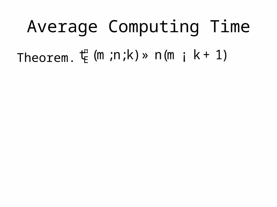
Average Computing Time

Theorem. t¤E (m;n;k) » n(m¡ k + 1)

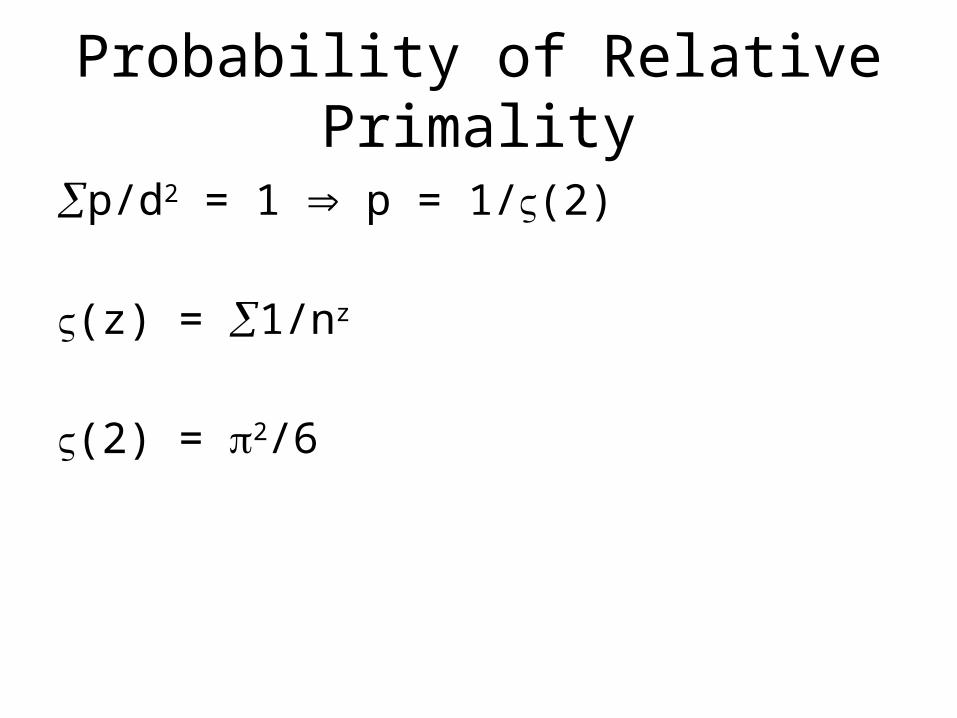
Probability of Relative Primality

p/d2 = 1 p = 1/(2)

(z) = 1/nz

(2) = 2/6

Formal Proof

Let qn be the number of 1 a,b n such that gcd(a,b) = 1. Then limn qn/n2 = 6/2

Mobius Function

• (1) = 1• (p1 pt) = -1t

• (n) = 0 if p2|n

(ab) = (a)(b) if gcd(a,b) = 1.

Mobius Inversion

d|n (d) = 0(n (n)ns)(n 1/ns) = 1

Formal Proof

qn = n (k)n/k2

limn qn/n2 = n (n)/n2 = 1/(n 1/n2) = 6/2

Assignment 1

• Empirically investigate distribution of quotients in Euclidean algorithm• Implement and analyze classical division algorithm• Implement and analyze Lehmer’s algorithm•Study and summarize gcd algorithms in GMP