Claremont CollegesScholarship @ Claremont

HMC Senior Theses HMC Student Scholarship

2001

Continued Fractions and their InterpretationsChristopher HanusaHarvey Mudd College

This Open Access Senior Thesis is brought to you for free and open access by the HMC Student Scholarship at Scholarship @ Claremont. It has beenaccepted for inclusion in HMC Senior Theses by an authorized administrator of Scholarship @ Claremont. For more information, please contactscholarship@cuc.claremont.edu.

Recommended CitationHanusa, Christopher, "Continued Fractions and their Interpretations" (2001). HMC Senior Theses. 127.https://scholarship.claremont.edu/hmc_theses/127

A Generalized Binet’s Formula for kth Order Linear

RecurrencesA Markov Chain Approach

byChristopher R. H. Hanusa

Francis Su, Advisor

Advisor:

Second Reader:

(Arthur Benjamin)

April 2001

Department of Mathematics

Abstract

A Generalized Binet’s Formula for kth Order Linear

Recurrences

A Markov Chain Approach

by Christopher R. H. Hanusa

April 2001

The Fibonacci Numbers are one of the most intriguing sequences in mathematics. I

present generalizations of this well-known sequence. Using combinatorial proofs,

I derive closed form expressions for these generalizations. Then using Markov

Chains, I derive a second closed form expression for these numbers which is a

generalization of Binet’s formula for Fibonacci Numbers. I expand further and

determine the generalization of Binet’s formula for any kth order linear recurrence.

Table of Contents

List of Figures iii

Chapter 1: Introduction 1

1.1 Tilings . . . . . . . . . . . . . . . . . . . . . . . . . . . . . . . . . . . . 1

1.2 Combinatorial Proofs . . . . . . . . . . . . . . . . . . . . . . . . . . . . 2

1.3 Markov Chains . . . . . . . . . . . . . . . . . . . . . . . . . . . . . . . 3

Chapter 2: Fibonacci Generalizations 5

2.1 Tiling Generalization . . . . . . . . . . . . . . . . . . . . . . . . . . . . 5

2.2 A Closed Form for Fk,n . . . . . . . . . . . . . . . . . . . . . . . . . . . 6

2.3 Specific Cases . . . . . . . . . . . . . . . . . . . . . . . . . . . . . . . . 6

2.4 A Tiling Interpretation of General Linear Recurrences . . . . . . . . . 7

2.5 Second Order Identities . . . . . . . . . . . . . . . . . . . . . . . . . . 9

Chapter 3: Binet-Like Formulas 12

3.1 Binet’s Formula for Fibonacci Numbers . . . . . . . . . . . . . . . . . 12

3.2 Generalization: Binet’s Formula for 3-omino Tilings . . . . . . . . . . 12

3.3 Markov Chain Model . . . . . . . . . . . . . . . . . . . . . . . . . . . . 14

3.4 Generalization: Binet’s Formula for k-omino Tilings . . . . . . . . . . 15

3.5 A Quick Check . . . . . . . . . . . . . . . . . . . . . . . . . . . . . . . 19

Chapter 4: Generalized Markov Chain Method 21

4.1 Easy kth Order Linear Recurrences . . . . . . . . . . . . . . . . . . . . 21

4.2 Making Sure . . . . . . . . . . . . . . . . . . . . . . . . . . . . . . . . . 23

4.3 Inclusion of Initial Conditions . . . . . . . . . . . . . . . . . . . . . . . 23

Chapter 5: Future Directions 26

5.1 p-ominoes and q-ominoes . . . . . . . . . . . . . . . . . . . . . . . . . 26

5.2 Whitney Numbers . . . . . . . . . . . . . . . . . . . . . . . . . . . . . 26

5.3 Conclusion . . . . . . . . . . . . . . . . . . . . . . . . . . . . . . . . . . 28

Bibliography 29

ii

List of Figures

1.1 An n× 1 board . . . . . . . . . . . . . . . . . . . . . . . . . . . . . . . 1

1.2 The two cases in Example 1. . . . . . . . . . . . . . . . . . . . . . . . . 3

3.1 The three Markov Chain states . . . . . . . . . . . . . . . . . . . . . . 14

4.1 an, 0 ≤ n ≤ k . . . . . . . . . . . . . . . . . . . . . . . . . . . . . . . . 24

iii

Acknowledgments

I would like to thank Professors Benjamin and Su for their support and helpful

comments and thought-provoking ideas. I would like to thank Tracy van Cort for

her LATEX knowledge and spirited moral support. And for random little things, I

would like to thank Anand Patil, Cam McLeman and Profs. Bernoff and Ward.

Thanks everyone!

iv

Chapter 1

Introduction

The inspiration for this thesis came two years ago when I was in a colloquium

listening to Jennifer Quinn speak about tilings and how they relate to Fibonacci

Numbers. Since then, combinatorial interpretations of tilings have inspired me

to ask many questions dealing with generalizations of such sequences. For this

thesis, I explain my year-long work, with Chapter 1, an introduction to the ideas

presented within, Chapter 2, a combinatorial proof of a closed form for the gener-

alized Fibonacci numbers, Chapter 3, a proof using Markov chains of a different

closed form for the same numbers, Chapter 4, where I generalize to a larger spec-

trum – all kth order linear recurrences, and Chapter 5, where I share my insights

into possible future work.

1.1 Tilings

In this paper we will use many tilings involving an n× 1 board tiled with squares

(1× 1 tiles) and dominoes (2× 1 tiles), as illustrated in Figure 1.1.

1 2 3 4 n...

Figure 1.1: An n× 1 board

2

Definition 1 Let fn denote the number of ways to tile this board with squares and domi-

noes.

Theorem 1.1.1 The recurrence formula for fn is fn = fn−1 + fn−2, for n ≥ 2.

Proof: The tiling of the n × 1 board can end in two possible tiles. Either it ends

with a square, in which case we can tile the rest of the (n − 1) × 1 board in fn−1

ways (by definition of fn−1), or it ends with a domino, in which case we can tile the

rest of the board in fn−2 ways. Thus, the number of ways to tile an n × 1 board is

fn−1 + fn−2. �

Since a board of length 0 has one tiling (the empty tiling) and a board of length

1 has one tiling, we have f0 = f1 = 1. Hence the fn’s are the Fibonacci numbers.

The standard Fibonacci sequence starts with F0 = 0, F1 = 1 and goes on from there;

thus fn = Fn+1. Summarizing, we have

Theorem 1.1.2 The number of ways to tile an n × 1 board with squares and dominoes is

the nth Fibonacci number, fn.

The structure of tiling the n×1 board in this way was used by Arthur Benjamin

and Jennifer Quinn in [4] and [2] as well as by Brigham et al in [5] to prove many

identities involving Fibonacci numbers.

1.2 Combinatorial Proofs

The general idea of a combinatorial proof is to show two quantities are equal by

counting the same set of objects in two different ways, thus establishing their

equality. As an example, we show how to prove a classic algebraic result of Fi-

bonacci using a combinatorial proof. (See [4].)

Example 1 f2n = f 2n + f 2

n−1

3

...

n n+1

... ...

...

1 2 2n-1 2n

Figure 1.2: The two cases in Example 1.

Proof: In this example, we want to count the number of ways to tile a board of

length 2n.

On one hand, this is the definition of f2n. In another respect, we can look at this

problem in two cases – there is either a break or no break between cells n and n+1,

as exhibited in Figure 1.2.

If there is a break, the number of ways to independently tile each half of the

board is fn, so the number of ways to tile the whole board is fn · fn = f 2n . If there is

no break, it is necessary that there be a domino covering cells n and n + 1, so there

are n−1 cells to tile on either half, and the number of ways to do this is fn−1 ·fn−1 =

f 2n−1. So the total number of ways to tile the 2n× 1 board is f2n = f 2

n + f 2n−1. Thus

the equality is established. �

In the following chapter, the reader will see similar techniques used to exhibit

other identities involving generalizations of Fibonacci numbers.

1.3 Markov Chains

In Chapters 3 and 4, I use the technique of Markov chains. A Markov chain is a

sequence of random variables on some state space, with a fixed probability pij of

moving from state i to state j at each step. This probability does not depend on

the past; only on the current state. Thus, given an object’s initial state, one can

determine the probability that the object is in any particular state at any time.

4

Example 2 Given the matrix M

M =

1 2 3 4 5

1 0 14

14

14

14

2 0 0 13

13

13

3 0 0 0 12

12

4 0 0 0 0 1

5 1 0 0 0 0

(1.1)

of transition probabilities and given that at time 0, the model starts in state 4, what is the

probability that the model is in state 2 at time 7?

Demonstration: In this example, we want to calculate M7 (representing seven time

steps) and apply it to the initial vector

x0 =[

0 0 0 1 0]

(1.2)

which represents our initial probabilities (we start in state 4 at time zero). Once we

do this, we arrive at the probability distribution at step 7 of:

x7 =[

0 0 0 1 0]

0 14

14

14

14

0 0 13

13

13

0 0 0 12

12

0 0 0 0 1

1 0 0 0 0

7

=[

1348

564

67576

53288

101288

](1.3)

From this, we see that the probability that the model is in state 2 at time 7 is 5/64.

We will use this Markov Chain approach more abstractly in Chapter 4.

Chapter 2

Fibonacci Generalizations

In this chapter, we see how to use tiling methods to generalize Fibonacci Num-

bers.

2.1 Tiling Generalization

To generalize the Fibonacci Numbers, we choose to tile an n×1 board with squares

and k-ominoes.

Definition 2 A k-omino is a tile that covers k cells.

Just like with Definition 1, we can now define a series of numbersFk,n that depends

on this constant k.

Definition 3 Let Fk,n denote the number of ways to tile an n× 1 board with squares and

k-ominoes.

Theorem 2.1.1 The sequence Fk,n can be defined recursively

Fk,n = Fk,n−1 + Fk,n−k (2.1)

with starting conditions

Fk,0 = Fk,1 = · · · = Fk,k−1 = 1. (2.2)

The proof to this is analogous to the proof of Theorem 1.1.1. The reader will note

that the specific case when k = 2 is exactly the Fibonacci sequence as exhibited in

Theorem 1.1.2.

6

2.2 A Closed Form for Fk,n

We have a recurrence relation for Fk,n, but it would be nice to have a closed form.

Here, from first principles of tilings, we derive such a closed form for Fk+1,n. (The

k + 1 is chosen for convenience, so the end result is easier to state.)

Lemma 2.2.1 The number of ways to tile an n×1 board using i (k +1)-ominoes is(

n−iki

)Proof: If you are tiling an n × 1 board using i (k + 1)-ominoes, then there are

n − i(k + 1) cells to place squares, and i k-ominoes to place, so in all, there is a

total of n − ik tiles to place, where i of them are k-ominoes. Since the squares are

indistinguishable from each other, as are the k-ominoes, we have established our

identity. �

Using this Lemma, we can establish a closed form for Fk+1,n, by summing over

all values of i; the number of ways to tile an n× 1 board with squares and (k + 1)-

ominoes is

Fk+1,n =∞∑i=0

(n− ik

i

). (2.3)

This theorem was proved by induction in the 1960’s by Hoggatt [14], but this result

is exciting because it was done combinatorially.

2.3 Specific Cases

To show that this is a reasonable generalization, we shall now cite some specific

cases of formula (2.3), letting k = 1 and k = 0.

If we let k = 1 then formula (2.3) becomes

F2,n = Fn =∞∑i=0

(n− i

i

). (2.4)

This is an algebraic result of the Fibonacci numbers that was recently proved com-

binatorially in [4].

7

If we let k = 0, consider what this means - we are tiling with squares and 1-

ominoes. So we are tiling with squares and alternate types of squares (we’ll give

them a different color) squares. The recurrence is

F1,n = F1,n−1 + F1,n−1 = 2F1,n−1, (2.5)

which is the recurrence for the powers of 2, which makes sense; at each cell we

have a choice of two colors, so the number of ways to cover n cells is 2n. By letting

k = 0 in Equation (2.3), we arrive at the identity

2n =∞∑i=0

(n

i

), (2.6)

which is the well-known fact that the sum of the elements of the nth row of Pascal’s

triangle is equal to 2n. In fact, Equation (2.4) is the sum of the diagonals of Pascal’s

triangle and Equation (2.3) is the sum of lines of slope k of Pascal’s triangle [6],[7].

In these specific cases, the simple elegance of the closed form is striking.

2.4 A Tiling Interpretation of General Linear Recurrences

When we deal with more types of tiles than just squares and dominoes, up to

length k, we will be dealing with a kth order linear recurrence.

Definition 4 A kth order linear recurrence is a sequence where each term in the se-

quence is a linear combination of the k previous terms.

The symbolic representation of a kth order linear recurrence is

an = c1an−1 + c2an−2 + · · ·+ ckan−k, (2.7)

where the ci are constant coefficients. For combinatorial purposes, the ci’s must be

non-negative integers. To define a specific series, we also need initial conditions,

let them be a0, a2, . . . , ak−1. Given these coefficients and initial conditions, our

8

linear recurrence is completely defined. Since we have 2k pieces of information to

take into account, it makes sense that we should have 2k types of tiles. First, to

take into account the coefficients, we remember the previous section, when we tile

a board with two types of squares. In that case, we used two different colors. We

can so a similar thing here – we now look at the tiling of an n × 1 board using c1

colors of squares, c2 colors of dominoes, . . ., up to ck colors of k-ominoes. To take

into account the initial conditions, we must be more clever. We will let the first tile

in any tiling (an i-omino) be special, giving it pi different phases. (We use phases to

distinguish them from colors, following the convention in [3].)

Definition 5 Let pi be the number of ways to tile the first tile if it is an i-omino.

We will now calculate pi in terms of the ai and ci. If an is to count the number

of ways to tile a board of length n with colored tiles as described above, we can

condition on the last tile. If n > k, we have an = c1an−1 + c2an−2 + · · · + ckan−k.

Now for n ≤ k, the last tile has length i where 1 ≤ i ≤ n. If i = n, then our tiling

consists of a single tile, for which there are pi choices. Otherwise there are cian−i

such tilings. Thus, for 1 ≤ n ≤ k, we must have that

an = pn + c1an−1 + c2an−2 + · · ·+ cn−1a1 = pn +n−1∑i=1

cian−i. (2.8)

Thus for a proper tiling interpretation, we must define for 1 ≤ n ≤ k,

pn = an −n−1∑i=1

cian−i. (2.9)

We can also make one further simplification: We will define a0 to satisfy

ak = c1ak−1 + c2ak−2 + · · ·+ cka0, (2.10)

in which case

pk = ak − c1ak−1 − c2ak−2 − · · · − ck−1a1 = cka0, (2.11)

9

and the empty board is tiled in a0 ways.

So given the k variable pi phases of the first tile and the k variable cj colors of

j-ominoes in the tiling, we now have the 2k variables we need for a tiling interpre-

tation of a kth order linear recurrence.

2.5 Second Order Identities

Using this newly found knowledge leads us to many identities proven at a glance

where they had not been before. We illustrate here the case when we have a gen-

eralized second order linear recurrence. Given non-negative integers a, b, H0, and

H1, the recurrence

Hn = aHn−1 + bHn−2 (2.12)

for n ≥ 2 can be given a combinatorial interpretation. Specifically, Hn counts the

number of tilings of an n×1 board with squares of a different colors and dominoes

of b different colors, and an initial square can be chosen in H1 possible ways and

an initial domino can be chosen in bH0 possible ways. Now let’s use this to prove

some identities!

Identity 1 b∑n

k=0 an−kHk = Hn+2 −H1an+1

Proof: This identity comes from counting the number of tilings of an (n + 2) × 1

board using at least one domino. The left hand side of the equation comes from

remarking that there must be a last domino. If the domino is to be in the last

position (i.e. covering cells n + 1 and n + 2), there are bHn ways to tile the board.

If the domino is in the second to last position, there are a square possibilities for

position n + 2, b possibilities for the domino in cells n and n + 1, and Hn−1 ways to

tile the rest of the board, for a total of baHn−1 tilings. In general, if the last domino

covers cells k + 1 and k + 2, then there are ban−kHk ways to create such a board.

Note that this expression is also valid when k = 0. This establishes the left side of

10

the equation. The right side is much simpler; there are Hn+2 total ways to tile the

board, and H1 · an+1 ways to tile the board using only squares. �

Identity 2 a∑n

k=1 bn−kH2k−1 = H2n −H0bn

Proof: Similar reasoning produces this identity, tiling a 2n× 1 board using at least

one square. Here we condition on the location of the last square. Note that the last

square can not be in an odd position, because then there would be an odd number

of cells afterwards to tile using only dominoes. Thus if the last square is to be in cell

2k (1 ≤ k ≤ n), there are H2k−1 ways to tile cells 1, . . . , k, a choices for the square in

cell 2k, and then bn−k ways to tile the remaining 2n− 2k cells with n− k dominoes.

Summing over all k yields the left side of the identity. The right side is shown by

noting that there are H2n total ways to tile the board, and bH0 · bn−1 ways to tile the

board using only dominoes. �

Similar reasoning produces: a∑n

k=1 bn−kH2k = H2n−1 −H1bn.

Identity 3 a∑2n

i=1 b2n−iHi−1Hi = H22n − b2nH2

0

Proof: Looking at the terms in the series on the left, we see that this identity is

different from before, in that we must use a pair of tilings, in order to achieve

an Hi−1Hi term. We accomplish this by taking an ordered pair of 2n-tilings, (A, B)

where A or B contains at least one square. The left hand side is seen by defining the

parameter kX to be the first cell of tiling X covered by a square. If X is all dominoes,

we set kX to infinity. Since there is at least one square, the minimum of kA and kB

must be finite and odd. Let k = min{kA, kB + 1}. When k is odd, A and B have

dominoes covering cells 1 through k − 1 and A has a square at cell k. In this way,

the number of tilings (A,B) with odd k is the number of ways to tile A times the

number of ways to tile B, i.e. ab(k−1)/2H2n−k · b(k−1)/2H2n−k+1 = abk−1H2n−kH2n−k+1.

When k is even, A has dominoes covering cells 1 through k and B has dominoes

covering cells 1 through k − 2 and a square at cell k − 1, so the number of tiling

11

pairs is bk/2H2n−k · ab(k−2)/2H2n−k+1 = abk−1H2n−kH2n−k+1. In this way, the left hand

side of the identity is satisfied. The right hand side is given when we look at the

number of pairs of 2n-boards without squares, in other words, the total number of

2n-board pairs ([H2n]2) minus the number of only domino-tiled boards ([H0bn]2). �

A similar technique yields: a∑2n+1

i=2 b2n+1−iHi−1Hi = H22n+1 − b2nH2

1 . This proof

can also be done using tail-swapping, a technique presented in [4].

The proofs of these identities were modeled after similar identities for a gen-

eralized Fibonacci sequence a = b = 1 proved by Benjamin, Quinn, and Su in [3].

These identities are immediately obvious from our tiling interpretation of a second

order linear recurrence, which evokes the practicality of this interpretation of such

systems.

Chapter 3

Binet-Like Formulas

In this chapter we discuss a generalization of Binet’s Formula for Fibonacci

Numbers.

3.1 Binet’s Formula for Fibonacci Numbers

In [1], Benjamin, Levin, Mahlburg, and Quinn give a novel proof of Binet’s formula

for Fibonacci numbers, which states that

Fn = F2,n−1 =1√5

[φn −

(−1

φ

)n]. (3.1)

where φ = 1+√

52

. The general idea they use is to randomly tile an infinitely long

board, placing a square with probability 1/φ and placing a domino with probability

1/φ2, and defining a new relation based on the probability t hat a new tile starts at

the nth cell.

Definition 6 We define a tiling to be breakable at cell n if a new tile starts at the nth cell.

In our random tiling of the infinite board, we let qn be the probability that a tiling

will be breakable at cell n.

3.2 Generalization: Binet’s Formula for 3-omino Tilings

Benjamin et al. [1] give several proofs of Equation (3.1), including an approach

using Markov chains. We apply the Markov chain approach to establish a gener-

alized Binet’s formula for Fk,n. We first show how to emulate their method for the

13

3-omino case, and then explain how it generalizes to the k-omino case. This will

give a closed form for the Fk,n numbers.

The reason why Benjamin et al. assigned the probabilities 1/φ and 1/φ2 for

placing squares and dominoes was to ensure that up to cell n, the probability of

any tiling is the same, 1/φn, and that the probability of choosing a tile at any step is

1/φ + 1/φ2 = 1. I suggest that φ (along with its counterpart −1/φ) is fundamental

in Fibonacci theory because 1/φ + 1/φ2 = 1, in the same way that we shall see that

the k roots of 1/χ + 1/χk = 1 are fundamental to the series Fk,n.

Let us study the F3,n case. We will place a square with probability 1/τ1, and

place a 3-omino with probability 1/τ 31 , where τ1 is the unique real root of

1

τ+

1

τ 3= 1. (3.2)

Thus, τ satisfies the characteristic equation

τ 3 − τ 2 − 1 = 0. (3.3)

This (positive) real τ exists because of Descartes’s Rule of Signs, which says that

the number of positive real roots of an equation is less than or equal to the number

of sign changes in the polynomial, and equal in parity. As there is only one sign

change, there must be this unique τ . Later we will use the other two (complex)

roots of this equation; denote them τ2 and τ3.

Let qn denote the probability that the tiling is breakable at cell n. Since there are

F3,n−1 ways to tile the first n − 1 cells, and each such tiling has probability 1/τn−11

of occurring, we see that

qn =F3,n−1

τn−11

. (3.4)

14

n

...

...

......

...

...

n-2 n+2n+1n-1

B0

B1

B2

Figure 3.1: The three Markov Chain states

3.3 Markov Chain Model

We will now come up with a formula for qn (and hence Fk,n) using a Markov chain

model. The process of randomly placing tiles can be described by a chain of states

that moves between three states: B0 (breakable at the current cell), B1 (a tile begin-

ning one cell before the current cell), and B2 (a tile beginning two cells before the

current one). (See Figure 3.3.)

The matrix of transition probabilities is as follows:

P =

B0 B1 B2

B0 1τ1

1τ31

0

B1 0 0 1

B2 1 0 0

(3.5)

where pij is the probability of going from state i to state j. Note the presence of 1’s

in the second and third rows. These occur because once a 3-omino is placed, there

is no choice; we must continue with the 3-omino until it is completed. We begin at

time (cell) 1 in the breakable state. So qn, the probability this tiling is breakable at

cell n, is the (1, 1) entry of P n−1. Using the diagonalization P = Q−1DQ,

15

P n−1 =

τ1

3τ1−2τ2

3τ2−2τ3

3τ3−2

τ13τ1−2

τ21

τ2(3τ2−2)

τ21

τ3(3τ3−2)

τ13τ1−2

τ13τ2−2

τ13τ3−2

(τ1τ1

)n−1

0 0

0(

τ2τ1

)n−1

0

0 0(

τ3τ1

)n−1

1 1τ31

1τ31

1 1τ21 τ2

1τ1τ2

2

1 1τ21 τ3

1τ1τ2

3

,

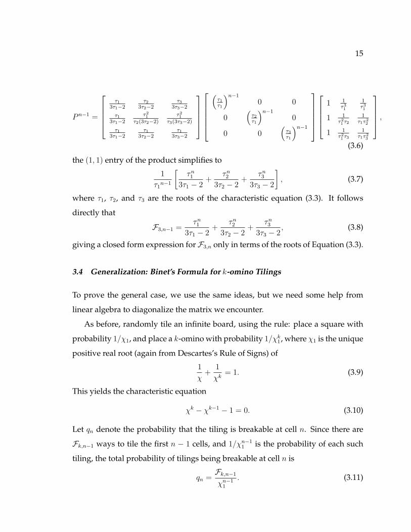
(3.6)

the (1, 1) entry of the product simplifies to

1

τ1n−1

[τn1

3τ1 − 2+

τn2

3τ2 − 2+

τn3

3τ3 − 2

], (3.7)

where τ1, τ2, and τ3 are the roots of the characteristic equation (3.3). It follows

directly that

F3,n−1 =τn1

3τ1 − 2+

τn2

3τ2 − 2+

τn3

3τ3 − 2, (3.8)

giving a closed form expression for F3,n only in terms of the roots of Equation (3.3).

3.4 Generalization: Binet’s Formula for k-omino Tilings

To prove the general case, we use the same ideas, but we need some help from

linear algebra to diagonalize the matrix we encounter.

As before, randomly tile an infinite board, using the rule: place a square with

probability 1/χ1, and place a k-omino with probability 1/χk1, where χ1 is the unique

positive real root (again from Descartes’s Rule of Signs) of

1

χ+

1

χk= 1. (3.9)

This yields the characteristic equation

χk − χk−1 − 1 = 0. (3.10)

Let qn denote the probability that the tiling is breakable at cell n. Since there are

Fk,n−1 ways to tile the first n − 1 cells, and 1/χn−11 is the probability of each such

tiling, the total probability of tilings being breakable at cell n is

qn =Fk,n−1

χn−11

. (3.11)

16

Our Markov chain will now move between k states: B0 (breakable at the current

cell), B1 (a tile beginning one cell before the current cell), and B2 (a tile beginning

two cells before the current one) as before, and then B3 to Bk−1 with Bi being the

state that a tile begins i cells before. Here, the matrix of transition probabilities is:

P =

B0 B1 B2 B3 · · · Bk−1

B0 1χ1

1χk

10 0 · · · 0

B1 0 0 1 0 0

B2 0 0 0 1...

...... . . . . . . 0

Bk−2 0 0 0 0 1

Bk−1 1 0 0 · · · 0 0

(3.12)

where pij is the probability of going from state i to state j. Note the diagonal of 1’s

just above the main diagonal. This occurs because once a k-omino is placed, there

is no choice; we must continue with the k-omino until it is completed. We begin at

time (cell) 1 in the breakable state. So qn, the probability we are breakable at time

n, is the (1, 1) entry of P n−1. We now want to diagonalize the probability matrix P :

P = Q−1 ·D ·Q. (3.13)

We recall from linear algebra [8] that the rows of Q and the columns of Q−1 consist

respectively of the right and left eigenvectors corresponding to the eigenvalues on

the diagonal of D. We first establish:

Theorem 3.4.1 The eigenvalues of the probability matrix P are χi/χ1 for 1 ≤ i ≤ k.

Proof: We return to the definition of eigenvalue, where since λI−A is a singular

17

matrix, it must have 0 determinant, i.e.

|λI − A| =

∣∣∣∣∣∣∣∣∣∣∣∣∣∣∣∣∣∣

λ− 1χ1

− 1χk

10 0 · · · 0

0 λ −1 0 0

0 0 λ −1...

... . . . . . . 0

0 0 0 λ −1

−1 0 0 · · · 0 λ

∣∣∣∣∣∣∣∣∣∣∣∣∣∣∣∣∣∣= 0 (3.14)

Evaluating the determinant using expansion by minors and multiplying each side

by λk yields,

λk − λk−1

χ1

+(−1)k(−1)k+1

χk1

= 0, (3.15)

where the (−1)k+1 term comes from the expansion by minors method. This gives

us

(λχ1)k − (λχ1)

k−1 − 1 = 0. (3.16)

By satisfying Equation (3.16), (λχ1) also satisfies the characteristic Equation (3.10),

so the k eigenvalues of P are related to the k roots of Equation (3.10). How cool is

that!

For each root χi of Equation (3.10), there is a corresponding eigenvalue λi satis-

fying χiλi = χ1 So, the k eigenvalues of P are

λi = χi/χ1 (3.17)

for 1 ≤ i ≤ k. �

Now that we know this, we can find column vectors vi and row vectors wi for

each eigenvalue satisfying

Pvi =χi

χ1

vi (3.18)

wiP =χi

χ1

wi (3.19)

18

We can determine vi:

1χ1

1χk

10 0 · · · 0

0 0 1 0 0

0 0 0 1...

... . . . . . . 0

0 0 0 0 1

1 0 0 · · · 0 0

v1

v2

...

vk

=

λiv1

λiv2

...

λivk

(3.20)

So,

λiv2 = v3λiv3 = v4...λivk = v1 (3.21)

Setting v1 = 1, we have the column vectors vi,

vi =

[1,

(χ1

χi

)k−1

,

(χ1

χi

)k−2

, . . . ,χ1

χi

]T

(3.22)

Similarly we can find wi,

wi =

[1,

1

χk−11 χi

,1

χk−21 χ2

i

, . . . ,1

χ1χk−1i

](3.23)

These eigenvectors determine Q and Q−1 up to constant factors. We calculate Q

and Q−1 independently because this is easier than taking the inverse of a k × k

matrix. Since this is the case we can form Q from the row vectors wi:

Q =

w1

w2

w3

...

wk

=

1 1χk

1

1χk

1· · · 1

χk1

1 1

χk−11 χ2

1

χk−21 χ2

2

1

χ1χk−12

1 1

χk−11 χ3

1

χk−21 χ2

3

1

χ1χk−13

... . . . ...

1 1

χk−11 χk

1

χk−21 χ2

k

· · · 1

χ1χk−1k

. (3.24)

19

We consolidate the constants ci into Q−1; form Q−1 from the column vectors vi:

Q−1 =[

c1v1 c2v2 c3v3 · · · ckvk

]=

c1 c2 c3 · · · ck

c1 c2χ1

χ2

k−1 c3χ1

χ3

k−1 . . . ckχ1

χk

k−1

c1 c2χ1

χ2

k−2 c3χ1

χ3

k−2 . . . ckχ1

χk

k−2

......

c1 c2χ1

χ2c3

χ1

χ3. . . ck

χ1

χk

.

(3.25)

Using QQ−1 = I , we can solve for the ci. This yields:

ci =χi

kχi − k + 1(3.26)

So the diagonalization P = Q−1DQ has been determined.

The (1, 1) entry of the product simplifies to

qn =1

χ1n−1

[χn

1

kχ1 − k + 1+

χn2

kχ2 − k + 1+ · · ·+ χn

k

kχk − k + 1

], (3.27)

where χ2, χ3, . . . , χk are the other k− 1 roots of our characteristic equation. Hence,

Fk,n−1 =χn

1

kχ1 − k + 1+

χn2

kχ2 − k + 1+ · · ·+ χn

k

kχk − k + 1(3.28)

giving a closed form expression for Fk,n in terms of the roots of Equation (3.10).

3.5 A Quick Check

Here we note that the general form reduces to Binet’s Formula for k = 2 as follows.

The characteristic polynomial in this case is

χ2 − χ− 1 = 0. (3.29)

The two roots of this equation are φ and −1/φ. So Equation (3.28) says the closed

form expression for Fn = F2,n−1 is

Fn =φn

2φ− 1+

(−1/φ)n

2 (−1/φ)− 1(3.30)

20

which reduces nicely to Binet’s formula for the Fibonacci numbers as presented at

the beginning of this chapter.

But that’s not all! In the next chapter, I explain how to generalize this formula

even further – any kth order linear recurrence.

Chapter 4

Generalized Markov Chain Method

Here we explore what happens to our Markov chain method if we do not re-

strict ourselves to tiling only with squares and k-ominoes, but allow a generalized

kth order linear recurrence.

4.1 Easy kth Order Linear Recurrences

In this section, we take the Initial Conditions of the linear recurrence to be that

which we would get if the pi phases are equal to the ci types of tiles, as explained

in Section 2.4. The first two terms, for example are a1 = c1 and a2 = c21 + c2. Later

we will generalize further.

From Equation (2.7), we have the determining characteristic equation

xk − c1xk−1 − c2x

n−2 − · · · − ck−1x− ck = 0, (4.1)

which we can use as the basis of our Markov Chain Method. We let µ1 be the

positive real root of Equation (4.1) that exists from Descartes’s Rule of Signs, and

let µ2, µ3, · · · , µk be the other roots. [Note that in Chapter 3, only ck and c1 were 1,

all the rest were 0.] We let the probability that we place an i-omino be ci

µi1. We now

note that the sum of the probabilities to place a tile is 1 since the sum is the same

as equation

c1µk−11 + c2µ

n−21 + · · ·+ ck−1µ1 + ck = µk

1, (4.2)

and by the definition of µ1, this equality holds. This Markov chain still moves

between the k states B0, B1, B2, . . . , Bk−1, where Bi is the state where the current

tile ends after n− i more cells, with the matrix of transition probabilities:

22

P =

(B0 B1 B2 B3 · · · Bk−1B0 c1

µ1

ck

µk1

ck−1

µk−11

ck−2

µk−21

· · · c1µ2

1B1 0 0 1 0 0B2 0 0 0 1

......

... . . . . . . 0Bk−2 0 0 0 0 1Bk−1 1 0 0 · · · 0 0

)(4.3)

where pij is the probability of going from state i to state j. To find the eigenvalues

λi of the matrix P , we take λI−P as singular, and we take the determinant to find:

|λI − P | = (λµ1)k − c1(λµ1)

k−1 − c2(λµ1)k−2 − · · · − ck−1(λµ1)− ck = 0. (4.4)

We now see a correlation to Theorem 3.4.1, where we can determine the eigenval-

ues of P with respect to the roots of our new characteristic equation, Equation (4.1).

By satisfying Equation (4.4), (λµ1) also satisfies the characteristic Equation (4.1), so

the k eigenvalues of P in this general case are

λi = µi/µ1 (4.5)

for 1 ≤ i ≤ k. From this information, we can diagonalize P as we did in (3.24) and

(3.25). This time,

vi =

[1,

(µ1

µi

)k−1

,

(µ1

µi

)k−2

, . . . ,µ1

µi

]T

(4.6)

and

wi =

[1,

ck

µk−11 µi

,ck−1µi + ck

µk−21 µ2

i

, . . . ,c2µ

k−2i + c3µ

k−31 + · · ·+ ck

µ1µk−1i

]. (4.7)

Now we find Q and Q−1 as before:

Q =

w1

w2

w3

...

wk

=

1 ck

µk1

ck−1+ck

µk1

· · · c2+c3+···+ck

µk1

1 ck

µk−11 µ2

ck−1µ2+ck

µk−21 µ2

2

c2µk−22 +c3µk−3

2 +···+ck

µ1µk−12

1 ck

µk−11 µ3

ck−1µ3+ck

µk−21 µ2

3

c2µk−23 +c3µk−3

3 +···+ck

µ1µk−13

... . . . ...

1 ck

µk−11 µk

ck−1µk+ck

µk−21 µ2

k

· · · c2µk−2k +c3µk−3

k +···+ck

µ1µk−1k

. (4.8)

23

Q−1 =[

v1 v2 v3 · · · vk

]=

d1 d2 d3 · · · dk

d1 cd2µ1

µ2

k−1 d3µ1

µ3

k−1 . . . dkµ1

µk

k−1

d1 d2µ1

µ2

k−2 d3µ1

µ3

k−2 . . . dkµ1

µk

k−2

......

d1 d2µ1

µ2d3

µ1

µ3. . . dk

µ1

µk

. (4.9)

Using QQ−1 = I , we can solve for the di. This yields:

di =µk

i

c1µk−1i + 2c2µ

k−2i + 3c3µ

k−3i + · · ·+ kck

(4.10)

Hence our diagonalization P = Q−1DQ is complete. This gives us a Binet’s for-

mula for kth order linear recurrences with simple initial conditions:

an =k∑

i=1

diµni . (4.11)

4.2 Making Sure

We now verify this formula matches the case I presented in Chapter 3, when only

ck and c1 were 1, all the rest were 0 and the initial conditions were a1 = 1, a2 =

1, a3 = 2, as required. Everything looks good in our comparison except perhaps

our constant factor di from Equation (4.10). Some algebra indeed verifies that

di =χk

i

χk−1i + k

=χi

kχi − k + 1. (4.12)

And from this we see that Equation (4.11) looks good.

4.3 Inclusion of Initial Conditions

Consider the series

αn = c1αn−1 + c2αn−2 + · · ·+ ck−1αn−k+1 + ckαn−k, (4.13)

where the ci’s are positive integers, but the first k terms, A0, A1, . . . , Ak−1 may be

of any type. To formulate a Binet’s Formula for such a wide range of recurrences,

24

Term an

0 1

1 c1

2 c1a1 + c2

3 c1a2 + c2a1 + c3

......

k − 1 c1ak−2 + c2ak−3 + · · ·+ ck−2a1 + ck−1

k c1ak−1 + c2ak−2 + · · ·+ ck−2a2 + ck−1a1

Figure 4.1: an, 0 ≤ n ≤ k

we approach the problem, hope to establish a set of “basis series” e0,n, e1,n, . . . ,

ek−1, n satisfying (4.13). In this way, every series with initial conditions A0, A1, . . . ,

Ak−1 can be represented as a linear combination of these basis series. For a specific

recurrence given ci, this series is determined by the first k terms, so it is easy to

verify that vectors of initial conditions determine a k dimensional vector space.

Choose the initial conditions of the basis series ei,n to be an n-vector with a 1 in the

ith position and 0’s elsewhere. We wish to now find the Binet’s Formula for these

basis series given the result in Equation (4.11). To accomplish this, we look at the

zero and negative terms of this series. Because of the simple way we recursively

define an, we can find these terms easily: a0 = 1 and a−1 = a−2 = · · · = a1−k = 0.

Now we look at the series an in Figure 4.1. What we can see is that to achieve a

basis series e0,n of initial conditions A0 = 1, A1 = A2 = · · · = Ak−1 = 0, we can take

e0,n = an − c1an−1 − c2an−2 − · · · − ck−1an−k+1. (4.14)

Similarly, we can find basis series 1 ≤ i ≤ k − 1,

ei,n = an−i − c1an−i−1 − c2an−i−2 − · · · − ck−i−1an−k+1. (4.15)

25

What we have done in effect is a row-echelon reduction of a k×k matrix of the ini-

tial conditions of the series an, . . . , an−k+1. From these basis series, we can represent

any kth order linear recurrence with initial conditions A0, A1, . . . , Ak−1 as

αn = A0e0,n + A1e1,n + A2e2,n + · · ·+ Ak−1ek−1,n, (4.16)

which is equal to

αn = A0[an−c1an−1−c2an−2−· · ·−ck−1an−k+1]+A1[an−1−c1an−2−· · ·−ck−2an−k+1]+A2[an−2−· · ·−ck−3an−k+1]+· · ·+Ak−1[an−k+1].

(4.17)

Collecting like terms gives us

αn = an[A0]+an−1[A1−c1A0]+an−2[A2−c1A1−c2A0]+· · ·+an−k+1[Ak−1−c1Ak−2−c2Ak−3−· · ·−ck−1A0].

(4.18)

And finally we can combine the Binet’s formulas for the aj linearly to achieve a

completely generalized Binet’s formula for kth order linear recurrences,

αn = A0

k∑i=1

diµni +(A1−c1A0)

k∑i=1

diµn−1i +(A2−c1A1−c2A0)

k∑i=1

diµn−2i +· · ·+(Ak−1−c1Ak−2−c2Ak−3−· · ·−ck−1A0)

k∑i=1

diµn−k+1i .

(4.19)

More easily represented,

αn =k∑

i=1

A0µki + (A1 − c1A0)µ

k−1i + · · ·+ (Ak−1 − c1Ak−2 − · · · − ck−1A0)µi

c1µk−1i + 2c2µ

k−2i + 3c3µ

k−3i + · · ·+ kck

µni .

(4.20)

Comparing my results to the Tribonacci sequence as outlined in [12] confirms

my solution in that specific case. YAY!

Chapter 5

Future Directions

In this chapter we discuss the continuation of these previous results and how

they may be applied elsewhere.

5.1 p-ominoes and q-ominoes

What happens if we don’t necessarily use squares as a tiling unit? What if we use

two types of rectangles, such as p-ominoes and q-ominoes. In this case, we derive

with a similar equation to formula (2.3).

Fpq,n =

∑i s.t.

q|n−ip

(n− ip

i

)=

∑j s.t.

p|n−jq

(n− jq

j

)(5.1)

The first equality can be seen in that n must equal ip+ jq for us to be able to tile

the n × 1 board with p-ominoes and q-ominoes. The second equality can be seen

similarly. In addition, this generalization jibes with the case when q = 1, because 1

always divides n− ip.

5.2 Whitney Numbers

In my studies so far, I have happened upon a number of identities that I have not

proved (yet), and so that these are not lost forever after I retire my thesis notebook,

I have included them here.

The most striking to me was an identity for the Whitney Numbers - an integral

part of the square/3-omino tiling. Here’s why:

27

When I was trying to generalize Binet’s formula using pure combinatorial meth-

ods, I wanted to come up with a form for qn as defined in Section (3.2) in terms of

a sequence that had the following form:

qn = a0,n − a1,n/τ3 + a2,n/τ

6 − · · ·+ an−1,n(−1/τ 3)n−1, (5.2)

trying to emulate another one of Benjamin et al.’s combinatorial methods of prov-

ing Binet’s formula.

What I found was intriguing! Instead of the nice geometric series that I was

hoping for, I found the Whitney numbers (w(n, k)) [11]. They are a set of numbers

that are defined

w(k, n) =k∑

i=0

(n

i

)(5.3)

I found that

ak,n = w(k, n− k). (5.4)

I then explored the Whitney numbers and their correlation with Pascal’s trian-

gle. I was extremely surprised to find out that I could sum variations of Pascal’s

triangle to come up with the Whitney numbers. Hence I came up with a new form

for Whitney numbers,

w(k, n) =∞∑i=0

(k + n− 2i

i

)(k + n− 3i

k − i

)(5.5)

which seems like a very different combinatorial relationship than what I’m used

to, so I have no idea how to prove it.

Now back to tilings. Then I wondered about the extension of these Whitney

Numbers into when you tile with squares and κ-ominoes, where I now define a

κ-Whitney number, wκ(n, k), as the coefficients of the (−1/χκ1) expansion of qn.

Here some unexpected patterns appeared. The most interesting property of the

κ-Whitney numbers is that

limκ→∞

wκ(n, k) =

(n

k

)(5.6)

28

so in other words, the limit of the κ-Whitney numbers is Pascal’s Triangle! I would

like to expand upon this further in the future.

5.3 Conclusion

I’ve described a number of different ideas, used combinatorics to prove new or pre-

existing identities involving Generalized Fibonacci Numbers, and the identities for

second-order linear recurrences, in Equation (2.3), and Identities 1, 2, and 3. I also

really enjoyed using Markov Chains to prove the pretty results of Binet’s Formulas,

in Equations (3.28), (4.11), and (4.20), and it makes me happy to know that these

have been done other ways, but I have a fresh new idea for these old theorems. If

I were to suggest things that needed more looking into, I would suggest trying to

find a correlation between my work and those by Spickerman and Joyner in [13]

and Mouline and Rachidi in [10] and [9]. I would also be interested in a modified

approach that would allow for non-integral coefficients in the recurrence. I think

that the connection between Whitney Numbers and Fibonacci Generalizations is

worth a look as well. I enjoyed the research that I did this year and hope that the

mathematical community can benefit. Bye for now.

Bibliography

[1] A. T. Benjamin, G. M. Levin, K. Mahlburg, and J.J. Quinn. Random Ap-

proaches to Fibonacci Identities. American Mathematical Monthly, 107(6):511–

516, 2000.

[2] A. T. Benjamin and J. J. Quinn. Fibonacci and Lucas Identities through Colored

Tilings. Fibonacci Quarterly, 30(5):359–366, 1999.

[3] A. T. Benjamin, J.J. Quinn, and F. E. Su. Phased Tilings and Generalized Fi-

bonacci Identities. The Fibonacci Quarterly, 38(3):282–288, 2000.

[4] A. T. Benjamin, F. E. Su, and J. J. Quinn. Counting on Continued Fractions.

Mathematics Magazine, 73:98–104, 2000.

[5] R. C. Brigham, R. M. Caron, P. Z. Chinn, and R. P. Grimaldi. A tiling scheme

for the Fibonacci numbers. J. Recreational Math., 28(1):10–16, 1996.

[6] M. Feinberg. New Slants. Fibonacci Quarterly, 2(3), 1964.

[7] A Generalization of the Connection Between the Fibonacci Sequence and Pas-

cal’s Triangle. Fibonacci Quarterly, 1(3):21–31, 1963.

[8] D. Lay. Linear Algebra and its Applications. Addison-Wesley-Longman, 2nd

edition, 1979.

[9] M. Mouline and M. Rachidi. Suites de fibonacci generalisees et chaınes de

markov. Revista de la Real Academia de Ciencias Exatas, Fisicas y Naturales de

Madrid, 89(1–2):61–77, 1995.

30

[10] M. Mouline and M. Rachidi. Application of Markov Chains properties to r-

Generalized Fibonacci Sequences. Fibonacci Quarterly, 30(1):34–38, 1999.

[11] On-line Encyclopedia of Integer Sequences. 2001. Available Online at

http://www.research.att.com/ njas/sequences/.

[12] W. R. Spickerman. Binet’s Formula for the Tribonacci Sequence. Fibonacci

Quarterly, 20(2):118–120, 1982.

[13] W. R. Spickerman and R. N. Joyner. Binet’s Formula for the Recursive Se-

quence of Order K. Fibonacci Quarterly, 22(4):327–331, 1984.

[14] Jr. V. E. Hoggatt. Combinatorial Problems for Generalized Fibonacci Num-

bers. Fibonacci Quarterly, 8(4):456–462, 1970.