Contextual Approach to Quantum Formalism || Contextual Probability and Interference

Chapter 3

Contextual Probability and Interference

The formula of total probability is one of the basic laws of classical probability

theory, see Part I: Chap. 2. In the case of two dichotomous random variables a =α1, α2 and b = β1, β2 it has the form

P(b = βi) = P(a = α1)P(b = βi |a = α1) + P(a = α2)P(b = βi |a = α2). (3.1)

On the other hand, we have a quantum analogue of this formula, see Part I: Chap. 1.

We call it the formula of total probability with the interference term

P(b = βi)

= P(a = α1)P(b = βi |a = α1) + P(a = α2)P(b = βi |a = α2)

+ 2 cos θ√

P(a = α1)P(b = βi |a = α1)P(a = α2)P(b = βi |a = α2),

(3.2)

where θ is the phase angle. This formula was derived in the formalism of complex

Hilbert space on the basis of Born’s postulate and the definition of quantum condi-

tional probability.

The Hilbert space derivation of the formula (3.2) might induce the impression

that we deal with something rather strange and impossible from the point of view of

classical probability theory. The appearance of the interference term has led to the

use of the term “quantum probability” in contradiction to what could be called “reg-

47

48 3 Contextual Probability and Interference

ular” or “classical” probability, see, e.g., [31, 38, 80, 82, 83, 92, 139], for extended

discussions on this problem.

In this chapter we provide contextual probabilistic analysis making a contribution

to the understanding of the formula of total probability and its violation.

Our analysis begins with the contextual definition of the relevant probabilities.

The probability for the value of one observable is then expressed in terms of the

conditional (contextual) probabilities involving the values of a second (“supplemen-

tary”) observable. In this way the interference term in the generalized formula of

total probability gives a measure of supplementarity of information which can be

obtained through measurements of observables a and b.1

The perturbing term in the generalized formula of total probability is then ex-

pressed in terms of a coefficient λ (probabilistic measure of supplementarity) whose

absolute value can be less than 1 or equal to 1, or it can be greater than one for

each of the values of the observable. This range of values for the coefficient λ then

introduces three distinct types of probabilistic perturbations:

(a) trigonometric, (b) hyperbolic, (c) hyper-trigonometric.

Each case is then examined separately. Classical (λ = 0) and quantum cases

(|λ| ≤ 1) are then special cases of more general results. Later it will be shown,

Chap. 4, that in the quantum case it is possible to reproduce a Hilbert space in

which the probabilities are found in the usual way, but there is a case in which this

is not possible, though the space is linear it is not a Hilbert space. In general it

is not a complex linear space. In the case of hyperbolic probabilistic behavior we

1 Of course, it would be better to use the terminology “complementarity of information.” How-

ever, N. Bohr had already reserved the notion of complementarity in quantum physics. The crucial

notion in Bohr’s complementarity (Copenhagen complementarity) is mutual exclusivity (incom-

patibility), see A. Plotnitsky [269–272] for an extended discussion, see also [187]. And in our

approach supplemental information which need not be based on incompatibility plays a crucial

role, see Sect. 3.4 of this chapter.

3.1 Växjö Model: Contextual Probability 49

have to use linear representation of probabilities over so-called hyperbolic numbers

(Part V).

3.1 Växjö Model: Contextual Probability

A general probabilistic model for observations based on the contextual viewpoint on

probability will be presented. It will be shown that classical (Kolmogorov and von

Mises) as well as quantum (Born-Dirac-von Neumann) probabilistic models can be

obtained as particular cases of our general contextual model—the Växjö model.

3.1.1 Contexts

In our model context C is any complex of conditions, e.g. physical or biological, or

social.

In principle, the notion of context can be considered as a generalization of a

widely used notion of preparation procedure, see, e.g., [29, 44]. However, identifi-

cation of context with preparation procedure would essentially restrict our theory.

In applications outside of physics (e.g., in psychology and cognitive science)

mental contexts are considered. Such contexts are not simply preparation proce-

dures. The same can be said about economic, political and social contexts. In this

book we shall not provide a deeper formalization of the notion of context. In our

model the notion of context is basic and irreducible, see [36, 235] for attempts to

formalize the notion of context.

Let us fix a set of contexts C which will be used in our model.

3.1.2 Observables

We now fix a set of observables O. We suppose that any observable a ∈ O can be

measured under a complex of physical conditions C.


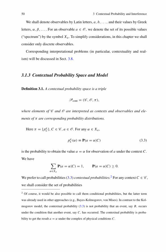
We shall denote observables by Latin letters, a, b, . . . , and their values by Greek

letters, α, β, . . . . For an observable a ∈ O, we denote the set of its possible values

(“spectrum”) by the symbol Xa. To simplify considerations, in this chapter we shall

consider only discrete observables.

Corresponding interpretational problems (in particular, contextuality and real-

ism) will be discussed in Sect. 3.8.

3.1.3 Contextual Probability Space and Model

Definition 3.1. A contextual probability space is a triple

Pcont = (C ,O, π),

where elements of C and O are interpreted as contexts and observables and ele-

ments of π are corresponding probability distributions.

Here π = {paC}, C ∈ C , a ∈ O. For any α ∈ Xa,

paC(α) ≡ P(a = α|C) (3.3)

is the probability to obtain the value a = α for observation of a under the context C.

We have∑

α∈Xa

P(a = α|C) = 1, P(a = α|C) ≥ 0.

We prefer to call probabilities (3.3) contextual probabilities.2 For any context C ∈ C ,

we shall consider the set of probabilities

2 Of course, it would be also possible to call them conditional probabilities, but the latter term

was already used in other approaches (e.g., Bayes-Kolmogorov, von Mises). In contrast to the Kol-

mogorov model, the contextual probability (3.3) is not probability that an event, say B, occurs

under the condition that another event, say C, has occurred. The contextual probability is proba-

bility to get the result a = α under the complex of physical conditions C.


W(O, C) = {P(a = α|C) : a ∈ O, α ∈ Xa}.

Definition 3.2. Contextual expectation E[a|C] of an observable a ∈ O with respect

to a context C ∈ C is given by

E[a|C] =∑

α∈Xa

αpaC(α).

Our probability model (“Växjö model”) will be based on the contextual probabil-

ity space having a sufficiently rich family of contexts—such that “transition proba-

bilities” P(b = β|a = α), a, b ∈ O, α ∈ Xa, β ∈ Xb, are well defined.

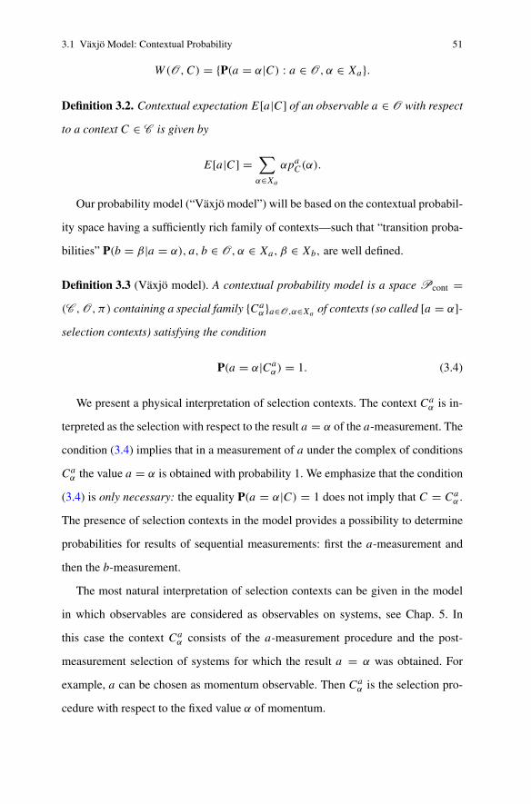
Definition 3.3 (Växjö model). A contextual probability model is a space Pcont =(C ,O, π) containing a special family {Ca

α}a∈O,α∈Xaof contexts (so called [a = α]-

selection contexts) satisfying the condition

P(a = α|Caα) = 1. (3.4)

We present a physical interpretation of selection contexts. The context Caα is in-

terpreted as the selection with respect to the result a = α of the a-measurement. The

condition (3.4) implies that in a measurement of a under the complex of conditions

Caα the value a = α is obtained with probability 1. We emphasize that the condition

(3.4) is only necessary: the equality P(a = α|C) = 1 does not imply that C = Caα.

The presence of selection contexts in the model provides a possibility to determine

probabilities for results of sequential measurements: first the a-measurement and

then the b-measurement.

The most natural interpretation of selection contexts can be given in the model

in which observables are considered as observables on systems, see Chap. 5. In

this case the context Caα consists of the a-measurement procedure and the post-

measurement selection of systems for which the result a = α was obtained. For

example, a can be chosen as momentum observable. Then Caα is the selection pro-

cedure with respect to the fixed value α of momentum.


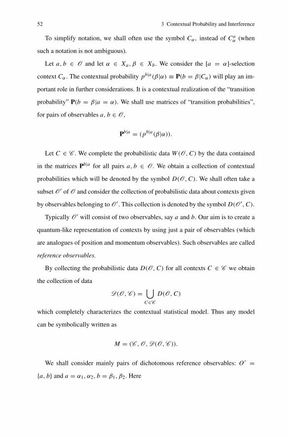
To simplify notation, we shall often use the symbol Cα, instead of Caα (when

such a notation is not ambiguous).

Let a, b ∈ O and let α ∈ Xa, β ∈ Xb. We consider the [a = α]-selection

context Cα. The contextual probability pb|a(β|α) ≡ P(b = β|Cα) will play an im-

portant role in further considerations. It is a contextual realization of the “transition

probability” P(b = β|a = α). We shall use matrices of “transition probabilities”,

for pairs of observables a, b ∈ O,

Pb|a = (pb|a(β|α)).

Let C ∈ C . We complete the probabilistic data W(O, C) by the data contained

in the matrices Pb|a for all pairs a, b ∈ O. We obtain a collection of contextual

probabilities which will be denoted by the symbol D(O, C). We shall often take a

subset O ′ of O and consider the collection of probabilistic data about contexts given

by observables belonging to O ′. This collection is denoted by the symbol D(O ′, C).

Typically O ′ will consist of two observables, say a and b. Our aim is to create a

quantum-like representation of contexts by using just a pair of observables (which

are analogues of position and momentum observables). Such observables are called

reference observables.

By collecting the probabilistic data D(O, C) for all contexts C ∈ C we obtain

the collection of data

D(O,C ) =⋃

C∈C

D(O, C)

which completely characterizes the contextual statistical model. Thus any model

can be symbolically written as

M = (C ,O,D(O,C )).

We shall consider mainly pairs of dichotomous reference observables: O ′ ={a, b} and a = α1, α2, b = β1, β2. Here


D(a, b, C) = {P(a = α|C), P(b = β|C), P(a = α|Cβ), P(b = β|Cα)},

where α = α1, α2 and β = β1, β2.

3.1.4 Växjö Models Induced by the Kolmogorov Model

Let P = (Ω,F , P) be a Kolmogorov probability space. It induces various Växjö

models through various choices of collections of contexts C and observables O as

well as systems of sets representing selection contexts for values of observables

from O.

The collection of contexts C can be chosen as some sub-family of F consisting

of sets of positive probability: P(C) > 0, C ∈ C . The crucial point is that the

collection of contexts need not form a σ -algebra or algebra.

The collection of observables O can be chosen as a subset of the space of random

variables RV (P). The crucial point is that not all random variables are chosen as

observables.3 In general O is only a proper subset of RV (P).

For a discrete variable a, its essential range of values (“spectrum”) is given by

the set Xa = {α}, where P(ω ∈ Ω : a(ω) = α) > 0.

Contextual probabilities in Växjö models induced by the Kolmogorov model are

given by the Bayes’ formula (so, these are simply conditional probabilities).

For an observable (random variable) a and its value α ∈ Xa the [a = α]-selection

context Cα can be chosen as the set Aα = {ω ∈ Ω : a(ω) = α}. The condition

(3.4) evidently holds. As was mentioned, this condition does not uniquely determine

selection contexts. In particular, we can choose any subset Aα of Aα (of strictly

positive probability) and still satisfy (3.4). What system of sets should be declared

as representing selection contexts depends on the problem under consideration. By

3 One may say that the Kolmogorov model provides the ontic description and the Växjö model

provides the epistemic description [27].


choosing various families of sets as representing selection contexts we create various

Växjö models. We remark that the choice of a proper subset Aα of the set Aα can be

justified by the physical situation—for example, by losses of particles in the process

of selection.

Another class of contextual probabilistic models can be induced by the Kol-

mogorov model via consideration on F of the equivalence relation given by the

condition4

P(C1ΔC2) = 0, (3.5)

and on the set RV (P) the standard equivalence relation for random variables: ξ is

equivalent to ξ ′ if

P(ω ∈ Ω : ξ(ω) �= ξ ′(ω)) = 0.

We now choose contexts and observables as equivalent classes of sets and random

variables, respectively. To determine a Växjö model, we fix families C and O of

corresponding equivalence classes. We remark that contextual probabilities are well

defined with the aid of the Bayes’ formula:

Let ξ, ξ ′ be equivalent random variables. It is easy to see that their essential

ranges of values coincide Xξ = Xξ ′ . Let U,U ′ be equivalent sets (of strictly positive

probability).

We set Aα ≡ Aξα = {ω ∈ Ω : ξ(ω) = α} and A′

α ≡ Aξ ′α = {ω ∈ Ω : ξ ′(ω) = α}.

First we remark that P(U) = P(U ′). We also have

P(Aα ∩ U) = P((Aα ∩ A′α ∪ Aα \ A′

α) ∩ (U ∩ U ′ ∪ U \ U ′))

= P(Aα ∩ A′α ∩ U ∩ U ′) = P(A′

α ∩ U ′).

Hence, P(ω ∈ Ω : ξ(ω) = α|U) = P(ω ∈ Ω : ξ ′(ω) = α|U ′). Thus P(a = α|C)

does not depend on choices of representatives ξ, ξ ′ ∈ a and U,U ′ ∈ C.

4 The symmetric difference of two sets is defined by C1ΔC2 = (C1 \ C2) ∪ (C2 \ C1).


Let a be an observable—an equivalence class of random variables. For any α ∈Xa, the selection context can be chosen (by such a choice we fix the model) by

the equivalence class of sets Aξα for ξ ∈ a. To show this, it is enough to see that

P(AαΔA′α) = 0 for ξ, ξ ′ ∈ a.

3.1.5 Växjö Models Induced by the Quantum Model

The set of contexts C can be chosen as a subset of the unit sphere S of complex

Hilbert space H : each context C ∈ C is encoded by a vector ψ ∈ S : C ≡ Cψ.

The set of observables O can be chosen as a subset of the space of self-adjoint

operators Ls(H ) having purely discrete5 nondegenerate6 spectra.

Contextual probabilities are defined by Born’s rule. Let an operator a ∈ O have

the spectrum Xa = {α1, . . . , αN , . . .}, αi �= αj and let eaα, α ∈ Xa, be correspond-

ing eigenvectors. Then

P(a = αi |Cψ) = |〈ψ, eaαi

〉|2.

The [a = α]-selection contexts Cα are represented by the eigenvectors: Cα ≡Cea

α. We have

P(b = β|Cα) = P(a = α|Cβ) = |〈eaα, eb

β〉|2.

We point out that transition probabilities in the Växjö model induced by QM are

very special. They are symmetric. In general the Växjö model produces nonsym-

metric transition probabilities (already the Växjö model induced by the Kolmogorov

model).

5 We recall that at the moment we have defined the Växjö model only for discrete observables, see

Chap. 6 for the “continuous generalization.”

6 We consider nondegenerate spectra to escape the problem of nonunique choice of selection con-

texts.


Another possibility to describe quantum probabilities within the contextual prob-

abilistic model is to proceed (similarly to the Kolmogorov case) by representing

contexts not by single vectors from the unit sphere S, but by equivalence classes of

these vectors: ψ1 is equivalent ψ2 if ψ1 = cψ2, where |c| = 1.

3.1.6 Växjö Models Induced by the von Mises Model

Consider a Växjö model (contextual probabilistic model) M = (C ,O,D(O,C )).

We would like to realize contextual probabilities of this model, π = {paC}C∈C ,a∈O,

in the frequency probabilistic framework.

Let C ∈ C be some context and let a, b ∈ O be two arbitrary observables. In a

series of observations of b under this context7 we obtain a sequence of values of b

x ≡ x(b|C) = (x1, x2, . . . , xN , . . .), xj ∈ Xb. (3.6)

In the same way we obtain a sequence of values of a

y ≡ y(a|C) = (y1, y2, . . . , yN , . . .), yj ∈ Xa. (3.7)

We suppose that these are S-sequences, see Definition 2.1, Part I: Chap. 2 (or even

von Mises collectives). Thus the principle of statistical stabilization holds and the

frequency probabilities are well defined

pb(β) = limN→∞ νN(β; x), β ∈ Xb, (3.8)

pa(α) = limN→∞ νN(α; y), α ∈ Xa, (3.9)

where νN(β; x) = n(β;x)N

, νN(α; x) = n(α;x)N

are relative frequencies of realizations

of labels b = β and a = α in sequences of observations x and y, respectively

7 Any context should be repeatable infinitely many times.

3.2 Contextual Probabilistic Description of Double Slit Experiment 57

(relative frequencies of observations of the results b = β and a = α under the

context C).

We define contextual probabilities of the Växjö model M as frequency probabil-

ities pbC(β) = pb(β) and pa

C(α) = pa(α).

We remark that it is not assumed that the observables a and b can be measured

simultaneously.

Let Cα be [a = α]-selection, α ∈ Xa. By observation of b under the context Cα

we obtain a sequence

xα ≡ x(b|Cα) = (x1, x2, . . . , xN , . . .), xj ∈ Xb. (3.10)

It is also assumed that the xα (α ∈ Xa) are von Mises collectives or at least S-

sequences. Thus the frequency probabilities with respect to the xα are well defined

pb|a(β|α) = limN→∞ νN(β; xα), (3.11)

where νN(β; xα) = n(β;xα)N

are relative frequencies of realizations of the label β in

xα (relative frequencies of observations of the result b = β under the context Cα).

One should consider a few different S-sequences (collectives) x, y, xα, α ∈ Xa,

which produce probability distributions

pbC(β), pa

C(α), pb|a(β|α). (3.12)

3.2 Contextual Probabilistic Description of Double Slit

Experiment

In this section we analyze the well-known double slit experiment from the contex-

tual probabilistic viewpoint. Denote by G a source of light, by U12 a screen with

two open slits, by Uj the same screen with only the j th open slit, j = 1, 2; by W a


screen covered by photoemulsion. We consider the following contexts

C12 = {G,U12,W }, Cj = {G,Uj ,W }, j = 1, 2,

We also consider observables:

b is the “momentum observable.” It is given by the position of a dot appearing

on the registration screen W. This position determines the direction of the photon’s

velocity.

a is the “position observable.” It is realized as the slit observable. To measure a,

we place two detectors dj , j = 1, 2 directly after slits. If dj produces a click then

a = j. If light has very low intensity, then two detectors practically never produce

clicks simultaneously.

Thus we consider the set of contexts C = {C12, C1, C2} and the set of observ-

ables O = {a, b}. The context Cj is selection with respect to the value a = j of the

a-observable: if we measure position a under the context Cj (i.e., only the j th slit

is open) then we get the value a = j with probability 1.

We consider the dichotomous version of the momentum observable. We choose

some domain on the registration screen and put b = 1 if a dot appears inside this

domain and b = 0 if a dot appears outside this domain. We consider the following

S-sequences (collectives):

x ≡ x(b|C12)—results of the b-measurement when both slits are open;

y ≡ y(a|C12)—results of the a-measurement when both slits are open;

xj ≡ x(b|Cj )— results of the b-measurement when only the j th slit is open,

j = 1, 2.

We obtain the probabilistic data

P(b = i|C12) = Px(b = i), P(a = j |C12) = Py(a = j),

pb|a(i|j) ≡ P(b = i|Cj ) = Pxj (b = i).

3.3 Formula of Total Probability and Measures of Supplementarity 59

3.3 Formula of Total Probability and Measures

of Supplementarity

Consider a Växjö model M = (C ,O,D(O,C )). Let C ∈ C be some context and

let a, b ∈ O be two arbitrary observables. For simplicity we assume that they are

dichotomous.

There are no reasons to assume the classical (Kolmogorovian) formula of total

probability, Part I: Chap. 2:

P(b = β) =∑

α

P(a = α)P(b = β|a = α) (3.13)

would be true for an arbitrary contextual probabilistic model. In principle, it can be

violated. We explain this point in more detail. In fact, all probabilities in (3.13) are

contextual. In (3.13) we omitted the indexes of contexts. However, in reality three

different contexts were involved. A context C is chosen for observations of a or b.

The following contextual probabilities are given: P(a = α) ≡ P(a = α|C), P(b =β) ≡ P(b = β|C). The selection contexts Cα, α ∈ Xa, are also involved. The

correct contextual definition of conditional probabilities in (3.13) is given by

P(b = β|a = α) = P(b = β|Cα).

In general there are no reasons to assume that probabilities with respect to the dif-

ferent contexts C,Cα should match the Kolmogorovian probabilistic law given by

the formula of total probability.

In the von Mises framework the formula of total probability holds for a partition

{Ak} of the label set L of a fixed S-sequence (collective) u

Pu(b = β) =∑

α

Pu(a = α)Pu(b = β|a = α). (3.14)

This formula can not be derived in the contextual probabilistic model with fre-

quency probabilities, where the conditional probabilities P(b = β|a = α) are de-


fined as contextual probabilities P(b = β|Cα). In this (contextual) approach differ-

ent S-sequences (collectives) are involved

x = x(b|C), y = y(a|C), xα = x(b|Cα), α ∈ Xa.

Thus, by using the contextual probabilistic model, in general one could not ex-

clude the possibility that the following probabilistic coefficient

δ(β|a, C) = Px(β) −∑

α

Py(α)Pxα (β) �= 0. (3.15)

As was mentioned, in the Kolmogorov or von Mises models, see (3.13), (3.14), we

have

δ(β|a, C) = 0. (3.16)

Definition 3.4. The quantity δ(β|a, C) is said to be a probabilistic measure of b|a-

supplementarity in the context C.

We can write the equality (3.15) in a form which is similar to the classical formula

of total probability

Px(β) =∑

α

Py(α)Pxα (β) + δ(β|a, C), (3.17)

or by using shorter notation

pb(β) =∑

α

pa(α)pb|a(β|α) + δ(β|a, C). (3.18)

This formula has the same structure as the quantum formula of total probability:

[classical part] + additional term,

cf. (3.2). To write the additional term in the same form as in the quantum represen-

tation of statistical data, we perform the normalization of the probabilistic measure

of supplementarity by the square root of the product of all probabilities

3.3 Formula of Total Probability and Measures of Supplementarity 61

λ(β|a, C) = δ(β|a, C)

2√∏

α pa(α)pb|a(β|α)

. (3.19)

The coefficient λ(β|a, C) also will be called the probabilistic measure of supple-

mentarity.

By using this coefficient we rewrite (3.18) in the QL form

pb(β) =∑

α

pa(α)pb|a(β|α) + 2λ(β|a, C)

√∏

α

pa(α)pb|a(β|α). (3.20)

The coefficient λ(β|a, C) is well defined only in the case when all probabilities

pa(α), pb|a(β|α) are strictly positive. We consider the matrix of transition proba-

bilities Pb|a = (pb|a(β|α)). We remark that the matrix Pb|a is always stochastic

∑

β

pb|a(β|α) = 1 (3.21)

for any α ∈ Xa.

Definition 3.5. A context C is said to be a-nondegenerate if

P(a = α|C) > 0

for all α ∈ Xa.

We remark that the context Caα is b-nondegenerate iff

pb|a(β|α) �= 0, β ∈ Xb. (3.22)

The representation (3.20) can be used only for nondegenerate contexts C and Caα.

We can repeat all previous considerations by changing b|a-conditioning to a|b-

conditioning. We consider contexts Cbβ corresponding to selections with respect to

values of the observable b. Probabilistic measures of supplementarity δ(α|b, C) and

λ(α|b, C), α ∈ Xa, can be defined. The contexts Cbβ are a-nondegenerate iff

pa|b(α|β) �= 0, α ∈ Xa. (3.23)


For nondegenerate contexts C and Cbβ, we have

pa(α) =∑

β

pb(β)pa|b(α|β) + 2λ(α|b, C)

√∏

β

pb(β)pa|b(α|β). (3.24)

Definition 3.6. Observables a and b are called probabilistically conjugate if (3.22)

and (3.23) hold.

Theorem 3.1. Let observables be probabilistically conjugate and let a context

C ∈ C be both a- and b-nondegenerate. Then quantum-like formulas of total prob-

ability (3.20) and (3.24) hold.

3.4 Supplementary Observables

Definition 3.7. Observables a and b are called b|a-supplementary in a context C if

δ(β|a, C) �= 0 for some β ∈ Xb. (3.25)

Lemma 3.1. For any context C ∈ C , we have

∑

β∈Xb

δ(β|a, C) = 0. (3.26)

Proof. We have

1 =∑

β∈Xb

pb(β) =∑

β∈Xb

∑

α∈Xa

pa(α)pb|a(β|α) +∑

β∈Xb

δ(β|a, C).

Since Pb|a is always a stochastic matrix, we have for any α ∈ Xa :∑

β∈Xbpb|a(β|α)

= 1. By using that∑

α∈Xapa(α) = 1 we obtain (3.26).

We point out that by Lemma 3.1 the coefficient δ(β1|a, C) = 0 iff δ(β2|a, C) =0. Thus b|a-supplementarity is equivalent to the condition δ(β|a, C) �= 0 both for

β1 and β2.

Definition 3.8. Observables a and b are called supplementary in a context C if they

are b|a or a|b supplementary

3.5 Principle of Supplementarity 63

δ(β|a, C) �= 0 or δ(α|b, C) �= 0 for some β ∈ Xb, α ∈ Xa. (3.27)

By Lemma 3.1. observables are supplementary iff the coefficient δ(β|a, C) �= 0

for all β ∈ Xb or the coefficient δ(α|b, C) �= 0 for all α ∈ Xa.

Let us consider a contextual probabilistic model with the set of contexts C . Ob-

servables a and b are said to be supplementary in this model if there exists C ∈ C

such that they are supplementary in the context C.

Observables a and b are called nonsupplementary in the context C if they are

neither b|a nor a|b-supplementary

δ(β|a, C) = 0 and δ(α|b, C) = 0 for all β ∈ Xb, α ∈ Xa. (3.28)

Thus in the case of b|a-supplementarity we have ( for β ∈ Xb)

pb(β) �=∑

α

pa(α)pb|a(β|α); (3.29)

in the case of a|b-supplementarity we have (for α ∈ Xa)

pa(α) �=∑

β

pb(β)pa|b(α|β); (3.30)

in the case of supplementarity we have (3.29) or (3.30). In the case of nonsupple-

mentarity we have both representations

pb(β) =∑

α

pa(α)pb|a(β|α), β ∈ Xb, (3.31)

pa(α) =∑

β

pb(β)pa|b(α|β), α ∈ Xa. (3.32)

3.5 Principle of Supplementarity

After the careful study of Bohr’s views on complementarity and especially discus-

sions with A. Plotnitsky (see also his works on Bohr’s complementarity [269–272]),

I found that by complementarity N. Bohr understood complementarity based on mu-


tual exclusivity. In the Växjö approach, mutual exclusivity of experimental condi-

tions is not important. The crucial role is played by supplementarity of information

in the sense of “additional information.”

The Principle of Supplementarity:

There exist physical observables, say a and b, such that for some context C they

produce supplementary statistical information. The classical formula of total prob-

ability is violated. Supplementarity of the observables a and b under the context C

induces interference of probabilities P(b = β|C) and P(a = α|C).

3.6 Supplementarity and Kolmogorovness

Let us consider a Växjö model and let a, b ∈ O be two dichotomous observables.

Definition 3.9. Probabilistic data D(a, b, C) is said to be Kolmogorovian if there

exists a Kolmogorov probability space P = (Ω,F , P) and random variables ξa

and ξb on P such that

pa(α) = P(ξa = α), pb(β) = P(ξb = β); (3.33)

pb|a(β|α) = P(ξb = β|ξa = α), pa|b(α|β) = P(ξa = α|ξb = β). (3.34)

Here the conditional probabilities are defined by the Bayes formula.

If data D(a, b, C) is Kolmogorovian, then the observables a and b can be repre-

sented by Kolmogorovian random variables ξa and ξb. We remark that Kolmogorov-

ness of statistical data in the sense of Definition 3.9 is not so natural from the

physical viewpoint. In fact, probabilities pa, pb, pb|a, pa|b correspond to different

complexes of physical conditions (contexts) C,Cα,Cβ. It would be more natural to

assume that each context determines its own Kolmogorov probability measure. Nev-

3.6 Supplementarity and Kolmogorovness 65

ertheless, Kolmogorovian data appear in many models, e.g., in classical statistical

physics.

Lemma 3.2. Data D(a, b, C) is Kolmogorovian if and only if

pa(α)pb|a(β|α) = pb(β)pa|b(α|β). (3.35)

Proof. (a) If data D(a, b, C) is Kolmogorovian then (3.35) is reduced to the equality

P(O1 ∩ O2) = P(O2 ∩ O1) for O1,O2 ∈ F .

(b) Let (3.35) hold true. We set Ω = Xa × Xb, where Xa = {α1, α2}, Xb ={β1, β2}. We define the probability distribution on Ω by

P(α, β) = pb(β)pa|b(α|β) = pa(α)pb|a(β|α);

and define the random variables ξa(ω) = α, ξb(ω) = β for ω = (α, β). We have

P(a = α) =∑

β

P(α, β) =∑

β

pa(α)pb|a(β|α)

= pa(α)∑

β

pb|a(β|α) = pa(α).

And in the same way P(b = β) = pb(β). Thus

P(a = α|b = β) = P(a = α, b = β)

P(b = β)= pb(β)pa|b(α|β)

pb(β)= pa|b(α|β).

And in the same way we prove that pb|a(β|α) = P(b = β|a = α).

We now investigate the relation between Kolmogorovness and nonsupplemen-

tarity. If D(a, b, C) is Kolmogorovian, then the formula of total probability holds

true and we have (3.28). Thus observables a and b are nonsupplementary (in the

context C). Thus:

Kolmogorovness implies nonsupplementarity

or as we also can say

Supplementarity implies non-Kolmogorovness.


However, in the general case nonsupplementarity does not imply that probabilis-

tic data D(a, b, C) is Kolmogorovian. Let us investigate in more detail the case

when both matrices Pa|b and Pb|a are double stochastic. We recall that a matrix

Pb|a = (pb|a(β|α)) is double stochastic if it is stochastic (so (3.21) holds) and,

moreover,∑

α

pb|a(β|α) = 1, β = β1, β2. (3.36)

3.6.1 Double Stochasticity as the Law of Probabilistic Balance

As was mentioned, the equality (3.21) holds automatically. This is a consequence of

additivity and normalization by 1 of the probability distribution.

However, the equality (3.36) is an additional condition on the observables a

and b. Thus by considering double stochastic matrices we choose a very special

pair of observables.

I propose the following physical interpretation of the equality (3.21). Since

pb|a(β|α2) = 1 − pb|a(β|α1),

the Cα1 and Cα2 contexts compensate each other in “preparation of the property”

b = β. Thus (3.36) could be interpreted as the law of probabilistic balance for the

property b = β. If both matrices Pb|a and Pa|b are double stochastic, then we have

laws of probabilistic balance for both properties: a = α and b = β.

3.6.2 Probabilistically Balanced Observables

Definition 3.10. Observables a and b are said to be probabilistically balanced if

both matrices Pb|a and Pa|b are double stochastic.


It is useful to recall the following well-known result about double stochasticity

for Kolmogorovian random variables:

Lemma 3.3. Let ξa and ξb be random variables on a Kolmogorov space P =(Ω,F , P). Then the following conditions are equivalent:

(1) The matrices Pa|b = (P(ξa = α|ξb = β)), Pb|a = (P(ξb = β|ξa = α)) are

double stochastic.

(2) Random variables are uniformly distributed

P(ξa = α) = P(ξb = β) = 1

2.

(3) Random variables are “symmetrically conditioned” in the following sense

P(ξa = α|ξb = β) = P(ξb = β|ξa = α), (3.37)

so Pa|b = Pb|a.

Proof. We set Ai = {ω ∈ Ω : ξa(ω) = αi} and Bj = {ω ∈ Ω : ξb(ω) = βj },j = 1, 2 (we recall that we consider dichotomous random variables). First we prove

that (3) is equivalent (2):

(a1) Let P(Ai |Bj ) = P(Bj |Ai). Then

P(A1B1)

P(B1)= P(B1A1)

P(A1),

P(A2B2)

P(B2)= P(B2A2)

P(A2),

P(A1B2)

P(B2)= P(B2A1)

P(A1).

(3.38)

Thus we obtain P(B1) = P(A1), P(A2) = P(B2), P(B2) = P(A1). Thus

P(B1) = P(B2) = 1/2 and P(A1) = P(A2) = 1/2. (3.39)

(b1) Starting with (3.39) we obtain (3.38) and consequently a, b-symmetry of

transition probabilities.

We now prove that (1) is equivalent (2):

(a2) Let P(B1|A1) = P(B2|A2), P(B1|A2) = P(B2|A1). Then


P(B1A1)

P(A1)= P(B2A2)

P(A2),

P(B1A2)

P(A2)= P(B2A1)

P(A1); (3.40)

P(A1B1)

P(B1)= P(A2B2)

P(B2),

P(A1B2)

P(B2)= P(A2B1)

P(B1). (3.41)

By these equations we obtain

P(B1)

P(A1)= P(B2)

P(A2),

P(B2)

P(A1)= P(B1)

P(A2).

So P(A2)P(A1)

= P(A1)P(A2)

. Thus we obtain (3.39).

(b2) Let (3.39) hold true. Then we have already proved that transition probabili-

ties are symmetric. Thus

P(Bi |A1) + P(Bi |A2) = P(A1|Bi) + P(A2|Bi) = 1

(since every matrix of transition probabilities is always stochastic).

In general the Kolmogorovian characterization of probabilistically balanced ran-

dom variables is not valid for observables of the Växjö model.

Proposition 3.1. A Kolmogorov model for data D(a, b, C) need not exist even in

the case of nonsupplementary probabilistically balanced observables having the

uniform probability distribution (for the context C).

Proof. Let us consider probabilistic data D(a, b, C) such that pa(α) = pb(β) =1/2 (here pa(α) ≡ P(a = α|C), pb(β) ≡ P(b = β|C)) and both matrices Pa|b

and Pb|a are double stochastic. Let us assume that pa|b(α|β) �= pb|a(β|α). Then by

Lemma 3.2, data D(a, b, C) is non-Kolmogorovian, but

2δ(α|β,C) = 1 −∑

β

pa|b(α|β) = 0, 2δ(β|α,C) = 1 −∑

α

pb|a(β|α) = 0.

It seems to be that symmetrical conditioning plays a crucial role in these consid-

erations.


3.6.3 Symmetrically Conditioned Observables

Take an arbitrary Växjö model.

Definition 3.11. Observables a, b ∈ O are called symmetrically conditioned if

pa|b(α|β) = pb|a(β|α). (3.42)

Lemma 3.4. If observables a and b are symmetrically conditioned, then they are

probabilistically balanced (so the matrices Pa|b and Pb|a are double stochastic).

Proof. We have that, e.g.,∑

β pa|b(α|β) = ∑β pb|a(β|α) = 1.

As we have seen in Proposition 3.1, probabilistically balanced observables need

not be symmetrically conditioned, cf. Lemma 3.3.

Proposition 3.2. Let observables a and b be symmetrically conditioned. Probabilis-

tic data D(a, b, C) is Kolmogorovian iff the observables a and b are nonsupplemen-

tary in the context C.

Proof. Suppose that a and b are nonsupplementary. We set

pb|a(1|1) = pb|a(2|2) = p and pb|a(1|2) = pb|a(2|1) = 1 − p

(we recall that by Lemma 3.4 the matrix Pb|a is double stochastic). By (3.31), (3.32)

we have

pa(αi) =∑

β

pb(β)pa|b(αi |β) =∑

β

∑

α

pa(α)pb|a(β|α)pa|b(αi |β)

=∑

α

pa(α)∑

β

pb|a(β|α)pb|a(β|αi).

Let us consider the case i = 1:

pa(α1) = pa(α1)(p2 + (1 − p)2) + 2pa(α2)p(1 − p)

= pa(α1)(1 − 4p + 4p2) + 2p(1 − p).


Thus pa(α1) = 1/2. Hence pa(α2) = 1/2. In the same way we get that pb(β1) =pb(β2) = 1/2. Thus the condition (3.35) holds true and there exists a Kolmogorov

model P = (Ω,F , P) for probabilistic data D(a, b, C).

Conclusion. In the case of symmetrical conditioning Kolmogorovness is equivalent

to nonsupplementarity.

Corollary 3.1. For symmetrically conditioned observables, probabilistic data D(a,

b, C) is Kolmogorovian iff the observables a and b are uniformly distributed

pa(α1) = pa(α2) = 1/2; pb(β1) = pb(β2) = 1/2.

3.7 Incompatibility, Supplementarity and Existence

of Joint Probability Distribution

The notions of incompatible and complementary variables are considered as syn-

onymous in the Copenhagen quantum mechanics. Moreover, compatibility (and

consequently noncomplementarity) is considered as equivalent to existence of the

joint probability distribution

P(α, β) = P(a = α, b = β).

The joint probability distribution can be interpreted as the probability distribution

for simultaneous measurement. The latter is always possible for compatible observ-

ables (represented by commutative operators).

We now consider similar questions for our Växjö model (as was pointed out, we

use the notion of supplementarity, instead of complementarity, since the latter has

already been reserved by N. Bohr).

3.7 Incompatibility, Supplementarity and Existence of Joint Probability Distribution 71

3.7.1 Joint Probability Distribution

The frequency definition of probability is the most appropriate for considerations in

this section.

By definition, observables a and b are compatible in a context C if it is possible

to perform a simultaneous observation of them under C. For any instant of time t,

a pair of values z(t) = (a(t), b(t)) can be observed. The sequence of results of

observations is well defined

z(a, b|C) = (z1, z2, . . . , zN , . . .), zj = (yj , xj ),

where yj = α1 or α2 and xj = β1 or β2. Observables a and b are incompatible in a

context C if it is impossible to perform a simultaneous observation of them under C.

Definition 3.12. Observables a and b are probabilistically compatible in a context

C if they are compatible in C and collectives (or S-sequences) y = y(a|C) and

x = x(b|C) are combinable, see Part I: Chap. 2.

Observables a and b are probabilistically compatible iff the sequence z(a, b|C)

is a collective (or an S-sequence).8 Thus there exists the frequency simultaneous

probability distribution

P(α, β) ≡ Pz(α, β) = limN→∞

nN(α, β; z)

N. (3.43)

Probabilistic compatibility implies Kolmogorovness of data D(a, b, C) and

hence nonsupplementarity.

8 In the opposite case observables are probabilistically incompatible.


3.7.2 Compatibility and Probabilistic Compatibility

In quantum physics compatibility of observables—the possibility to perform a si-

multaneous observation—is typically identified with probabilistic compatibility—

existence of the frequency simultaneous probability distribution (3.43). It is a nat-

ural consequence of the Kolmogorovian psychology. In the frequency probability

theory we should distinguish compatibility and probabilistic compatibility.

We present an example in which observables are compatible (so they can be mea-

sured simultaneously), but the limit (3.43) does not exist. Here observables are not

probabilistically compatible. Of course, this means that S-sequences (collectives)

y = y(a|C) and x = x(b|C) are not combinable.

Differences between compatibility and probabilistic compatibility will play an

important role in analysis of Bell’s considerations, Part III. Bell did not differ be-

tween these two notions. Such a position induced misunderstanding of the inter-

relation between the possibility to use the realistic description for quantum correla-

tions and violation of Bell’s inequality.

We shall use some well-known results about the generalized probability given by

the density of natural numbers, see [139]. For a subset A ⊂ N, where N is the set of

natural numbers, the quantity

P(A) = limN→∞

|A ∩ {1, . . . , N}|N

is called the density of A if the limit exists. Here the symbol |V | is used to denote

the number of elements in the finite set V.

Let G denote the collection of all subsets of N which admit density. It is evident

that each finite A ⊂ N belongs to G and P(A) = 0. It is also evident that each subset

B = N\A, where A is finite, belongs to G and P(B) = 1 (in particular, P(N) = 1).

The reader can easily find examples of sets A ∈ G such that 0 < P(A) < 1. The

“generalized probability” P has the following properties:

3.7 Incompatibility, Supplementarity and Existence of Joint Probability Distribution 73

Proposition 3.3. Let A1, A2 ∈ G and A1 ∩ A2 = ∅. Then A1 ∪ A2 ∈ G and

P(A1 ∪ A2) = P(A1) + P(A2).

Proposition 3.4. Let A1, A2 ∈ G . The following conditions are equivalent

(1) A1 ∪ A2 ∈ G ; (2) A1 ∩ A2 ∈ G ;(3) A1 \ A2 ∈ G ; (4) A2 \ A1 ∈ G .

There are standard formulas

P(A1 ∪ A2) = P(A1) + P(A2) − P(A1 ∩ A2);P(A1 \ A2) = P(A1) − P(A1 ∩ A2).

It is possible to find sets A,B ∈ G such that, for example, A ∩ B �∈ G . Let A be

the set of even numbers. Take any subset C ⊂ A which has no density. In fact, you

can find C such that1

N|C ∩ {1, 2, . . . , N}|

is oscillating. There happen two cases: C ∩ {2n} = {2n} or = ∅. Set

B = C ∪ {2n − 1 : C ∩ {2n} = ∅}.

Then, both A and B have densities 1/2. But A ∩ B = C has no density. Thus G is

not a set algebra.

We now consider a context C which produces natural numbers. We introduce two

dichotomous observables

a(n) = IA(n), b(n) = IB(n),

where IO(x) is the characteristic function of a set O. We assume that these observ-

ables are compatible: we can, e.g., look at a number n and find both values a(n) and


b(n).9 We obtain two S-sequences

y = y(a|C) = (y1, . . . , yN , . . .),

x = x(b|C) = (x1, . . . , xN , . . .), yj , xj = 0, 1.

The frequency probability distributions are well defined

pa(α) ≡ Py(α) = 1/2, pb(β) ≡ Px(β) = 1/2.

However, the S-sequences y and x are not combinable. Thus observables a and b

are not probabilistically compatible; for example, the frequency probability P(1, 1)

does not exist.

A philosopher may say that the observables a and b are real. However, as we have

pointed out, realism (compatibility) does not imply probabilistic realism (probabilis-

tic compatibility).

3.8 Interpretational Questions

3.8.1 Contextuality

It is necessary to discuss the meaning of the term contextuality, as it can obviously

be interpreted in many different ways, see, e.g., Karl Svozil [294, 295] and espe-

cially [296] for details. The most common meaning (in QM and quantum logic,

[35], and especially in consideration of Bell’s inequality [34]) is that the outcome

for a measurement of an observable u under a contextual model is calculated using

a different (albeit hidden) measure space, depending on whether or not compatible

observables v,w, . . . were also made in the same experiment.

9 We can consider natural numbers as systems and interpret a(n) and b(n) as values of observables

a and b on the system n.

3.8 Interpretational Questions 75

We remark that the well-known “no-go” theorems (of, e.g., Bell) cannot be ap-

plied to such contextual models.

In our approach the term contextuality has an essentially more general meaning.

Physical context is any complex of physical conditions.

In particular, one can create a context by fixing the values of observables v,w, . . .

which are compatible with u. However, in this way we can obtain only a very special

class of contexts.

Thus the Växjö contextual model will cover the conventional quantum contextual

model, but it can be applied for observations which could not be described by the

quantum model.

3.8.2 Realism

We remark that in general the Växjö model does not contain physical systems (see

Chap. 5 for a special class of models in which contexts are represented by ensembles

of physical systems, see also Ballentine [29]). At the moment we do not (and need

not) consider observables as observables on physical systems. It is only supposed

that:

If a context C is fixed, then we can perform a measurement of any observable

a ∈ O under this complex of conditions.

In general we do not try to assign objective properties to a physical system and

consider observables as giving quantitative values of these objective properties. To

measure a ∈ O, one should first determine a context a ∈ O for measurement. If a

context is not determined, then it is meaningless to speak about measurement. Thus

the Växjö model is very general and it can be applied to practically all statistical

measurements in any domain of science (in particular, it covers quantum measure-

ments).


On the other hand, we would like to check how far it would be possible to proceed

by keeping to realism. We show that practically all quantum probabilistic effects,

e.g., the interference of probabilities and even the violation of Bell’s inequality, can

be described in the realistic (contextual) framework.

3.9 Historical Remark: Comparing with Mackey’s

Model

From the mathematical point of view our probabilistic model is quite close to the

well-known Mackey’s model. George Mackey [239] presented a program of huge

complexity and importance:

To deduce the probabilistic formalism of quantum mechanics starting with a sys-

tem of natural probabilistic axioms.

(Here “natural” has the meaning of a natural formulation in classical probabilistic

terms.) Mackey tried to realize this program starting with a system of 8 axioms—

Mackey axioms, see [239]. This was an important step in clarification of the prob-

abilistic structure of quantum mechanics. However, he did not totally succeed, see

[239] for details. The crucial axiom (about the complex Hilbert space) was not for-

mulated in natural (classical) probabilistic terms.

As Mackey [239] pointed out, probabilities cannot be considered as abstract

quantities defined outside any reference to a concrete complex of physical con-

ditions C. All probabilities are conditional, or better to say contextual.10 Mackey

did a lot to unify classical and quantum probabilistic description and, in particular,

10 We remark that the same point of view can be found in the works of A.N. Kolmogorov and

R. von Mises. However, it seems that Mackey’s book [239] was the first thorough presentation of

a program of conditional probabilistic description of measurements, both in classical and quantum

physics.

3.9 Historical Remark: Comparing with Mackey’s Model 77

demystify quantum probability. One crucial step is however missing in Mackey’s

work. In his book Mackey [239] introduced the quantum probabilistic model (based

on the complex Hilbert space) by means of a special axiom (Axiom 7, p. 71) that

looked rather artificial in his general conditional probabilistic framework.

Mackey’s model is based on a system of eight axioms, when our own model re-

quires only two axioms. Let us briefly mention the content of Mackey’s first axioms.

The first four axioms concern conditional structure of probabilities, that is, they can

be considered as axioms of a classical probabilistic model. The fifth and sixth ax-

ioms are of a logical nature (about questions). We reproduce below Mackey’s “quan-

tum axiom”, and Mackey’s own comments on this axiom (see [239], pp. 71–72):

Axiom 7 (Mackey). The partially ordered set of all questions in quantum mechanics

is isomorphic to the partially ordered set of all closed subsets of a separable, infinite

dimensional Hilbert space.11

Our activity can be considered as an attempt to find a list of physically plausible

assumptions from which the Hilbert space structure can be deduced. We showed

that this list can be presented in the form of a compact definition of the contextual

probabilistic model, see Sect. 3.1.

11 “This axiom has rather a different character from Axioms 1 through 4. These all had some

degree of physical naturalness and plausibility. Axiom 7 seems entirely ad hoc. Why do we make

it? Can we justify making it? What else might we assume? We shall discuss these questions in turn.

The first is the easiest to answer. We make it because it “works”, that is, it leads to a theory which

explains physical phenomena and successfully predicts the results of experiments. It is conceivable

that a quite different assumption would do likewise but this is a possibility that no one seems to

have explored. Ideally one would like to have a list of physically plausible assumptions from which

one could deduce Axiom 7.”


3.10 Subjective and Contextual Probabilities

in Quantum Theory

From the probabilistic viewpoint (by the Växjö interpretation) quantum mechanics

is a generalization of Bayesian statistical analysis based on the formula of total

probability. The classical Bayesian analysis is based on the classical formula of total

probability and “quantum Bayesian analysis” is based on the interference formula

of total probability.

If the coefficients of supplementarity λ(β|a, C) = 0, β ∈ Xb, then for b|a-

conditioning under the complex of physical conditions C we can use the classical

Bayesian analysis, if |λ(β|a, C)| ≤ 1, β ∈ Xb, then we can use the Hilbert space

variant of Bayesian analysis (which coincides with the classical one for observables

which are not supplementary under the context C), see Chap. 4.

If |λ(β|a, C)| ≥ 1, β ∈ Xb, then we could not use the classical Bayesian analy-

sis nor its complex Hilbert space generalization, but it is possible to use hyper-

bolic Bayesian analysis based on the formula of total probability with the cosh-

interference, see Part V.

From this point of view it is not surprising that quantum mechanics (its proba-

bilistic part) induced a strong tendency toward idealism. Even the classical Bayesian

analysis induced a similar tendency. In fact, the subjective interpretation of proba-

bility was developed starting with the Bayesian statistical analysis.

It should be expected that quantum mechanics would sooner or later induce the

subjective interpretation of quantum probabilities. And it really has happened, see

recent investigations of C. Fuchs, M. Appleby, A. Caticha, J.-A. Larsson, R. Schack,

see, e.g., [24, 49, 95, 96, 278] on the subjective probabilistic approach to quantum

foundations and quantum information. We remark that these investigations are to-

tally justified from the purely mathematical viewpoint (as well as investigations on

classical subjective probability), because they are based on the correct formalism.

3.10 Subjective and Contextual Probabilities in Quantum Theory 79

This is nothing wrong with De Finetti’s approach from a purely mathematical view-

point. The only unfair assumption is that the initial probability distribution in the

Bayesian analysis is chosen subjectively.

As was pointed out already by Kolmogorov [222] and Gnedenko [100], the

choice of the initial probability distribution is based on the results of previous ex-

periments. Statistical data which was collected in such experiments gives one the

possibility to propose some form of a priori probability distribution. For example,

when one uses the hypothesis that the distribution is Gaussian it is not just his purely

subjective proposal. It is, in fact, the result of the frequency data from the huge num-

ber of statistical experiments.

There is nothing wrong with the use of subjective probability as the basis of

an experimental statistical methodology. The main negative consequence of this ap-

proach is that it can support idealist views on physics (quantum as well as classical).

Therefore Kolmogorov [222] and Gnedenko [100] criticized so strongly the use of

subjective probability in science.

Documents

Contextual Approach to Quantum Formalism || Contextual Probability and Interference