Context Preserving Maps of Tubular Structures

Joseph Marino, Wei Zeng, Xianfeng Gu, and Arie Kaufman, Fellow, IEEE

(a) (b) (c)

Fig. 1. Context preserving map of a colon. (a) The original colon mesh from a standard view point. (b) The projected 2D skeleton ofthe colon after untangling and spacing. (c) The context preserving flattened map of the colon surface based on the 2D skeleton in (b).

Abstract—When visualizing tubular 3D structures, external representations are often used for guidance and display, and such viewsin 2D can often contain occlusions. Virtual dissection methods have been proposed where the entire 3D structure can be mappedto the 2D plane, though these will lose context by straightening curved sections. We present a new method of creating maps of3D tubular structures that yield a succinct view while preserving the overall geometric structure. Given a dominant view plane forthe structure, its curve skeleton is first projected to a 2D skeleton. This 2D skeleton is adjusted to account for distortions in length,modified to remove intersections, and optimized to preserve the shape of the original 3D skeleton. Based on this shaped 2D skeleton,a boundary for the map of the object is obtained based on a slicing path through the structure and the radius around the skeleton. Thesliced structure is conformally mapped to a rectangle and then deformed via harmonic mapping to match the boundary placement.This flattened map preserves the general geometric context of a 3D object in a 2D display, and rendering of this flattened map can beaccomplished using volumetric ray casting. We have evaluated our method on real datasets of human colon models.

Index Terms—Geometry-based technique, volume rendering, biomedical visualization, medical visualization, conformal mapping.

1 INTRODUCTION

A common application in visualization is to navigate inside a tubularstructure in order to inspect its walls, such as in virtual colonoscopy.In providing such a navigation, it is often desirable to maintain an ex-ternal view of the object so that one’s position within it can be easilydetermined. This is especially important when the structure looks sim-ilar at different regions. However, using a typical 3D model for thispurpose leads to its own problem, where sections can occlude eachother when they exist in the same region on the viewing plane and atdifferent depths along the view direction (see Figures 1a and 2). Suchproblems necessitate rotation of the 3D structure. We present here amethod of producing flattened maps of the surface which preserve the

• The authors are with the Computer Science Department at Stony Brook

University. E-mail: {jmarino, zengwei, gu, ari}@cs.stonybrook.edu.

Manuscript received 31 March 2011; accepted 1 August 2011; posted online

23 October 2011; mailed on 14 October 2011.

For information on obtaining reprints of this article, please send

email to: tvcg@computer.org.

geometric context, so that they can be used to guide navigation withinthe structure, but do not contain intersections which would cause oc-clusions.

A flattened representation of a structure can be useful for provid-ing an overview of the entire structure in a single 2D view. However,common methods of creating such views will straighten the object,such that it is difficult to locate where positions would correspond toby simply looking at the flattened representation. This is evident, forexample, in the case of flattening a colon to a long linear strip. Thoughthe 3D colon structure is often classified into separate sections basedon the major bends it contains, this information is lost in the flattenedrepresentation. In this work, we aim to preserve such geometric con-text of 3D structures in their 2D flattened representations.

Our method is based on first shaping the skeleton curve of the struc-ture within a 2D plane. The 3D skeleton is orthogonally projected toan optimal viewing plane. Given this projection, the 2D skeleton is ad-justed to ensure that the length along it is correct. Intersections of theskeleton are then removed and the spacing between skeleton segmentsis adjusted so that neighboring areas are not so close to each other. Afinal smoothed version is created to reduce high frequency noise along

1997

1077-2626/11/$26.00 © 2011 IEEE Published by the IEEE Computer Society

IEEE TRANSACTIONS ON VISUALIZATION AND COMPUTER GRAPHICS, VOL. 17, NO. 12, DECEMBER 2011

Fig. 2. Colon surface from Figure 1 viewed from above. From this van-tage point, it is easy to see how two long sections of the colon occludeeach other when viewed from the front or back.

the skeleton. This 2D skeleton will still maintain the general geometriccontext of the structure (see Figure 1b).

Given this 2D skeleton of the structure, it is then used as a guidein placing the location of the boundary of the object for the flattenedmap. The structure is sliced open, and each point along its boundaryis associated with a point along the skeleton. Using the radius of thestructure along the skeleton, the boundary is embedded in the plane.

Once the boundary of the flattened map has been computed, the 3Dsurface can be mapped to the plane using harmonic mapping. Har-monic mapping is chosen so that the boundary can be predefined with-out being a canonical shape. The mesh, now flattened to the plane,can then be rendered with volumetric ray casting to give a view of theinner surface of the entire structure.

The resulting context preserving flattened map is then readily usablefor guiding navigations, as the user is able to identify geometric land-marks that would otherwise be lost in a flattening map that has beenstraightened. Performing such a mapping can also make more intu-itive use of display real estate space. For example, a flattened colonthat has been straightened would require a very long display or a verythin representation. Using a context preserving flattening, the map willrequire less contiguous screen space in a single direction.

The paper is organized as follows. Section 2 presents related worksdealing with curve skeletons and flattening. In Section 3 we discuss themethod for shaping the 2D skeleton of the structure. Section 4 explainsthe placement of the boundary for the flattened surface in relation tothe 2D skeleton. Section 5 details the mapping of the surface from 3Dto 2D using harmonic mapping and its subsequent visualization. Wediscuss our results in Section 6 and conclude the paper in Section 7.

2 RELATED WORK

Extracting a skeleton curve of an object is a popular method of com-pactly representing the general geometric shape of the structure. Muchwork has been done over the years on methods of extracting theseskeleton curves. Skeleton extraction from volumetric medical data byconnecting centerlines based on a medial voxel path has been pre-sented [22]. A method has been proposed using a distance fromboundary field with penalty weights to obtain general skeletons of tree-like structures [2]. Obtaining a skeleton directly from a mesh by con-tracting the surface, without any need for a volumetric representation,has been suggested [9]. Both surface and curve skeletons from genus0 structures have been extracted through the use of advection to movemass from the object’s surface to its skeleton [12]. The use of leastsquares optimization has been suggested for extracting curve skele-tons in an efficient manner which is insensitive to noise [18]. Curveskeletons can also be approximated for data from incomplete pointclouds based on a generalized rotational symmetry axis for a set ofpoints [15].

There are many uses for skeleton curves in the fields of computergraphics and visualization, and their 1D representation of 3D objectsis useful for compact shape descriptions, navigation, animation, andanalysis [3]. Skeleton curves can be used to drive shape deforma-tions [19]. They have also been used in describing shape to allow

for the creation of shape-based transfer functions [11]. They are com-monly used for navigation in endoscopic visualizations, such as virtualcolonoscopy [17], and accurate curves are important for such kinds ofnavigation [16].

The use of conformal geometry for mapping triangular meshes,where local angles are preserved, has been well established in the fieldof computer graphics, especially in the creation of texture maps [14].Discrete Ricci flow is a more recent method of computing conformalmaps of structures [8]. There are many applications where discreteRicci flow is useful, such as in surface parameterization for texturemapping and construction of geometric structures [7] as well as to ob-tain optimal surface parameterizations using inverse curvature maps[20]. Applications of Ricci flow will typically use a target Gaussiancurvature of zero everywhere, or constrain the boundary to a canonicalshape, such as a disc.

Flattening tubular structures is a method of displaying the entire in-ner surface of the objects in a succinct 2D image and has been usedsuccessfully for several medical imaging applications. For the colon,it has been proposed to virtually unfold the surface by rendering rayscylindrically around the centerline [1]. A similar technique that alsopreserves some z-depth information along the flattened mesh has beenproposed [10]. Conformal mapping of the colon surface to the planehas also been utilized for triangular mesh models [4], and conformalmapping with volume rendering for image generation has been pre-sented [5]. Likewise, similar techniques have been applied to flat-ten vessels in an angle preserving manner [23]. In addition to usingflattening techniques simply for the purposes of visual display, thesetechniques have also been used for analysis of the surfaces. Com-puter aided detection of colonic polyps based on volume rendering ona conformally flattened colon image has been presented [6]. The useof quasi-conformal mapping for the registration of supine and pronecolon surfaces has also been suggested [21].

In this work, we use the flattened representation to present to theuser a visual display of the structure. Unlike previous works, whereflattened views straighten the structure along a line, we generate theflattened representation such that the geometric context is preserved,allowing the user to easily identify at what location in the original3D structure a position is. We use the skeleton curve as a basis fordescribing the geometric shape of the structure. We combine the useof discrete Ricci flow and harmonic mapping in this pipeline.

3 SKELETON LAYOUT

The creation of a context preserving map is based upon manipulatingthe skeleton of the structure, which can be found using any of thestandard methods [2, 3]. Given the 3D skeleton, it is first projectedto an optimal 2D plane. This projection is then corrected for length,untangled to remove intersections, and spaced properly to prevent self-intersections of the structure’s surface. The details of each of thesesteps follow. All operations are performed on a discretized version ofthe skeleton with initial equal spacing between points.

3.1 Orthogonal Projection

The original 3D skeleton of the structure is first projected to a plane,such that all z values become 0. Since this projection is to be usedas the basis for a map, perspective distortion is unnecessary and evendetrimental, and thus orthogonal projection is used. The projection isperformed using the standard orthogonal projection matrix:

[

x′

y′

]

=

[

ux uy uz

vx vy vz

]

xyz

, (1)

where u and v are the right and up vectors of the projection plane.The projection plane is chosen to be an optimal viewing plane for

the structure. For most types of objects, especially in medical appli-cations, a canonical view is known which provides the best view andis familiar to the user. If such a view is not known a priori, a planewhich minimizes structural overlap and skeletal intersections can beused. The 2D projected skeleton of a colon is shown in Figure 3a.

1998 IEEE TRANSACTIONS ON VISUALIZATION AND COMPUTER GRAPHICS, VOL. 17, NO. 12, DECEMBER 2011

(d)

(a) (b) (c) (e)

Fig. 3. Skeleton of the human colon shown in Figure 1. When intersections along the skeleton are present, alternating regions between intersectionsare colored black and red. (a) Projected 2D skeleton. (b) Lengthened projected 2D skeleton. (c) Untangled skeleton. (d) Close-up of an intersectionregion from (b). (e) Close-up of the same region from (c). Note that though from a distance the skeleton in (c) still appears to have intersections,they are in actuality just locations where the skeleton sections are very close.

3.2 Lengthening

When performing the orthogonal projection, the lengths of portions ofthe skeleton can be substantially diminished if the segment directionis aligned with the view direction of the projection plane. The closerto parallel the segment direction and view direction are, the greater theloss of length. To recover this length in the 2D skeleton, a lengtheningprocedure is applied that bends a straight skeleton with even spacinginto the shape of the projected skeleton.

For every point along the projected skeleton (except endpoints), itstwo neighboring skeleton points are used to create two vectors v1 andv2, and the angle between them is calculated in the standard way basedon the law of cosines:

θ = cos−1 v1 · v2

|v1||v2|. (2)

All of the points in the skeleton are then set in a straight line, withequal spacing between them equivalent to the original spacing of the3D discretized skeleton. Starting at beginning, the corresponding an-gle θ is used to rotate all following points p = (x,y) around the currentpoint p0 = (x0,y0) as follows:

[

x′

y′

]

=

[

cosθ −sinθsinθ cosθ

][

x− x0

y− y0

]

+

[

x0

y0

]

. (3)

If the original rotation was clockwise instead of counterclockwise inrelation to the normal of the projection plane, then the transpose ofthe matrix is used accordingly. This is performed for all points alongthe skeleton until the end is reached. After this process, the length ofthe skeleton from its original 3D shape is preserved, while the geo-metric structure of the projected 2D skeleton is also preserved. Thelengthened 2D skeleton of a colon is shown in Figure 3b.

3.3 Untangling

Given the lengthened 2D projected skeleton, it is then necessary tountangle it so that no intersections are present. This process, however,should maintain the general shape of the structure (compare Figures3b-c). This is done by looking for three types of intersections: loops,

crossings, and abutments. An example of each type of intersection andthe corresponding result of untangling is shown in Figure 4. The threetypes of intersections are as follows:

Abutment: An abutment (see Figure 4a) occurs when a center pointamong three consecutive discrete skeleton points lies on the op-posite side of another line segment of the skeleton than the othertwo points. This causes both line segments formed by the threepoints to intersect the skeleton at a single line segment, and thuscontains two points of intersection.

Loop: A loop (see Figure 4b) occurs when a skeleton comes aroundand crosses over itself without any other intersections within theformed loop. This creates one intersection point.

Crossing: A crossing (see Figure 4c) occurs when two sections ofa skeleton intersect each other without any loops or abutmentsbetween them. This contains two intersection points.

To remove these intersections, all intersections of the skeleton arefirst found. Each intersection is actually located twice within the list,once for each time it is encountered when tracing the path. The list ofintersections is then searched to locate the three different types listedabove. Given that an intersection is made of two intersecting line seg-ments in the discrete case, each intersection is represented by fourpoints, the first two points representing the endpoints of the first linesegment and the second two points representing the endpoints of thesecond line segment along the skeleton. The points themselves are or-dered as their order along the skeleton. Each of the three intersectionscan be identified as follows:

Abutment: An abutment is located by finding two consecutive inter-sections for the same line segment (intersecting two separate linesegments).

Loop: A loop is located as two consecutive intersections where thepair of line segments for the two intersections is the same.

1999MARINO ET AL: CONTEXT PRESERVING MAPS OF TUBULAR STRUCTURES

(a) Abutment

(b) Loop

(c) Crossing

Fig. 4. Types of intersections and their untangling results.

Crossing: A crossing is located as two consecutive intersections thatdo not meet either of the above two conditions.

After searching the list of intersections, the first intersection of thehighest priority that is found is corrected. The intersections in orderfrom high to low priority are abutment, loop, and crossing. Each typeof intersection is corrected as follows:

Abutment: An abutment is removed by simply setting the offendingpoint to the average of its two neighbor points.

Loop: A loop is removed by first creating a line segment from theloop intersection point to the median point of the loop. All pointswithin the loop are then reflected through this line segment tountangle it.

Crossing: A crossing is removed similarly to a loop. A line segmentspanning the two intersection points is found. All points withinthe crossing, on both segments of the skeleton, are then reflectedthrough this line segment to untangle it.

Since performing one correction can cause new intersections toarise, the skeleton is searched again after every correction procedureto find all intersections. This is repeated until no intersections arefound along the skeleton. After untangling, the skeleton is iterativelysmoothed to remove small sharp features (see Figure 5a).

3.4 Spacing

After the untangling procedure, several segments can lie very closeto each other due to the orientation of the projection plane. Theseclose areas must be spaced out so that there is room for the colon sur-face boundary when flattened. The radius of the structure along theskeleton is recorded, and the 2D skeleton points are translated perpen-dicular to their direction such that the radius segment from every pointdoes not intersect other sections of the skeleton. For each offset of theskeleton points, if an intersection is created, the offset is undone. Inthis way, no new intersections will occur. Neighboring skeleton pointsare also moved slightly to help avoid sharp bends. At the end, iterativesmoothing is applied to the entire skeleton to yield a clean path. Anexample of the result of this process is shown in Figure 5b.

(a) (b)

Fig. 5. Refined 2D skeleton of the colon shown in Figure 1. (a) Thesmoothed version of the untangled 2D skeleton. (b) The spaced andsmoothed version of the 2D skeleton.

4 BOUNDARY PLACEMENT

Given the untangled skeleton path of the structure, it is necessary toplace the boundary for the flattened surface in relation to it. In addi-tion to preserving the overall shape of the structure, we also wish torepresent the general size of structure along the skeleton. We accom-plish this by calculating the approximate radius along the skeleton andusing it to control the layout of the boundary. This has the effect ofcondensing the surface perpendicular to the skeleton, but the overallrelation of size between regions can still be observed.

4.1 Slicing

In order to map a tubular structure to a plane, it is necessary for thestructure to have a single boundary. The structure is discretely repre-sented by a closed surface triangular mesh (i.e., without boundaries),which is initially topologically equivalent to the sphere in R

3 (it has anEuler characteristic number χ = 2). To make the surface instead topo-

logically equivalent to a plane in R3, it must be sliced open from one

end to the other, creating a single boundary. Although this boundarycould technically be located anywhere, it should match the skeleton onthe original structure.

To locate the path along which the mesh is to be sliced open, Dijk-stra’s shortest path algorithm is used. This is advantageous for struc-tures with features such as bumps and valleys, through which the cut-ting line should not pass, as Dijkstra’s algorithm naturally tends toavoid these areas and instead locate a path along more uniform re-gions. In the case of the colon, for example, this means that the slicingpath will generally not go through features such as the haustral folds.For Dijkstra’s algorithm, the starting point is taken to be the vertex onthe surface mesh nearest to one end of the 3D skeleton. The targetpoint can then be taken as usual as the surface vertex with the great-est distance from the source. Alternatively, the surface vertex locatednearest to the other end of the skeleton can be taken as the target.

Given a path along the surface to use for slicing the surface open,two small holes are punched at each end of the path by removing oneface for each. This yields a structure that is now topologically equiva-lent to a cylinder (χ = 0). Slicing along the cutting path is now equiv-alent to slicing a cylinder from one boundary to another, yielding asurface with a single boundary (χ = 1) which is topologically equiva-lent to the plane. For every vertex along the slicing path, a new vertex

2000 IEEE TRANSACTIONS ON VISUALIZATION AND COMPUTER GRAPHICS, VOL. 17, NO. 12, DECEMBER 2011

(a) (b)

Fig. 6. Slicing path (shown in blue) on the 3D surface of the colon shownin Figure 1. (a) Front view. (b) Back view.

is duplicated with the same surface position. The sliced surface withthe boundary in blue is shown in Figure 6.

4.2 Skeletal Correspondence

As the boundary vertices are mapped to a surface around the 2D skele-ton, it is necessary for each boundary vertex to have a correspondenceto a position along the skeleton. Two corresponding boundary vertices(i.e., an original vertex from the unsliced mesh and a newly createdvertex from the slicing at the same position) are both associated withthe same position along the skeleton. The four end vertices on theboundary that result from punching holes at each end are treated ascorner points and are not associated with the skeleton, as they do notcontribute to the mapped shape. For all boundary vertices (other thancorresponding pairs as mentioned), no two boundaries can be associ-ated with the same location along the skeleton.

Since the twists and turns of a structure can often lead to situationswhere the closest skeletal point for a boundary vertex is actually in aseparate section, the location of correspondences between the skele-ton and boundary is created based on finding the nearest boundarypoint for each skeleton point, determining boundary to skeleton corre-spondences from those, and then interpolating positions for boundarypoints which were not indicated by a skeleton point. The correspon-dences are determined for the set of original surface vertices on theslicing path, and then duplicated to the newly created vertices. Thefirst and last vertices along the slicing path are mapped to the first andlast position along the skeleton. The algorithm is as follows:

for all skeleton points doFind nearest boundary vertex

end forfor all vertices on slicing path do

Find all skeleton points indicated as correspondencesTake center of those points as true correspondence

end forfor all vertices on slicing path without correspondence do

Interpolate neighborsend for

The correspondences (excluding the two end points) are thensmoothed through several iterations by setting the current boundary’scorrespondence position to the average of its two neighbors. The re-sults of this correspondence are shown in Figure 7.

4.3 Radius Along Skeleton

The radius for each point along the skeleton is determined based onthe correspondence with the boundary vertices explained above. Thealgorithm is as follows:

Fig. 7. Correspondence between boundary vertex points and skeletonpoints. The skeleton path is shown in green, the slicing path in red, andthe connections between a boundary point and the skeleton in blue.

for all skeleton points s dofor all boundary vertices v do

if v corresponds to segment containing s thenAccumulate weighted distanceAccumulate weight

end ifend for

end forfor all skeleton points do

if weight is not zero thendivide distance by weight

end ifend forfor all skeleton points without radius do

Interpolate neighborsend for

The radii of the skeleton points are then iteratively smoothed (againexcluding the endpoints) by averaging each skeleton point’s radius andits two neighbors.

4.4 Boundary Position

The position of the boundary is determined for every boundary vertex.For every vertex on the slice path (original vertices and newly createdvertices), the boundary location on the 2D map for a vertex vi is calcu-lated based on the discrete 2D skeleton points preceding and followingthe vertex’s location on the skeleton. The positions of these before andafter points are p1 = (p1x, p1y) and p2 = (p2x, p2y), and the radii forof the two points are r1 and r2, respectively. The normalized distancefrom p1 is represented by α . The new mapped position p for eachvertex on the slice path is calculated as follows:

n = p1− p2,

d =

[

dx

dy

]

=

[

ny

−nx

]

,

p0 = p1∗ (1−α)+ p2∗α ,

r = r1∗ (1−α)+ r2∗α ,

p =

{

p0+d ∗ r, ∀vi ∈ M0

p0−d ∗ r, ∀vi /∈ M0,

(4)

where M0 is the original unsliced mesh. The boundary points not onthe slice path (from when the holes were punched) are set to equalintervals between the nearest sliced vertices. A smoothing operation isapplied to remove intersections that might occur, while still preservingthe overall general geometric structure. An example of the boundaryfor the mapping is shown in Figure 8.

2001MARINO ET AL: CONTEXT PRESERVING MAPS OF TUBULAR STRUCTURES

Fig. 8. Placement of the boundary in 2D for the colon in Figure 1. Thenarrow portion is caused by a narrowing in the original mesh (see inset).

5 SURFACE MAPPING

Given the projected and spaced 2D skeleton of the structure and theboundary placement generated as the target domain S2, we map theoriginal 3D sliced colon surface S1 to the plane. Such mapping pre-serves the original projected curved information.

Discrete Ricci flow is used to map the open surface S1 to a rectan-gle D1 conformally, φ1 : S1 → D1. Similarly, the target domain S2 ismapped to another rectangle D2 conformally, φ2 : S2 →D2. Using har-monic mapping, we compute the one-to-one and onto correspondenceD1 and D2, h : D1 → D2. Finally, we lift the 2D correspondence tothe 3D surfaces, f : S1 → S2, and map the original 3D surface to thedesigned target domain. The pipeline is shown in Equation 5.

The final result can then be rendered either using mesh renderingwith vertex normal information stored from the original structure, orusing volume rendering through the original volumetric dataset, whichis the preferred method.

S1f

−−−−−→ S2

φ1

y

y

φ2

D1h

−−−−−→ D2

(5)

5.1 Ricci Flow

To map the 3D surface to the 2D plane, discrete Ricci flow is used.Ricci flow is a powerful tool for geometric analysis, and it has beenused to successfully prove the Poincare conjecture. It behaves like aheat diffusion, deforming one Riemannian metric to another Rieman-nian metric conformally, as shown in Equation 6:

dg

dt=−Kdt (6)

where g is the Riemannian metric and K is the target curvature. A fulldescription of the method of discrete Ricci flow for mapping triangularmeshes is outside the scope of this paper [8].

For the sliced colon surface, the boundary sides between each twocorners are mapped to a straight segment, and the four corners aremapped to be the right corners of a rectangle. At the same time, the

Fig. 9. Colon surface mapped to a rectangle. The four sections from topto bottom combine to form a single strip from left to right of the entirecolon.

(a)

(b)

Fig. 10. Example conformal modules (the ratios between height andwidth for the conformal mappings) for (a) the original surface (0.045796)and (b) the target domain (0.015378).

interior surface is mapped conformally to the plane. Therefore, for dis-crete Ricci flow, we set the target curvature of four corners to be π

2 andthe curvatures of other boundary vertices and interior vertices to be 0.The result of this is a rectangular mapping, as shown in Figure 9. Sim-ilarly, for the generated target domain, we compute the correspondingcorner vertices and boundary sides, set the same target curvature, andobtain its conformal rectangular mapping. As a mesh is needed forthis, we use the 2D boundary samples as constraints and perform aconstrained Delaunay triangulation [13] to generate the triangular tar-get domain.

5.2 Deformation

Now we compute the one-to-one and onto correspondence betweentwo rectangles by minimizing the harmonic energy. The resulting har-monic mapping obtains the smoothest deformation between two rect-angles. In general, the original 3D colon surface S1 and the 2D targetdomain S2 are not conformally equivalent. As shown in Figure 10,their conformal modules (the ratios between height and width for theconformal mappings D1 and D2) are quite different.

From the computation of the target boundary placement, the corre-spondence of boundary vertices is known. The positions of the targetboundary vertices are then used as the constrained condition in theharmonic mapping, as shown in the following equations:

harmonic energy E = ∑edge(i, j)∈D2

‖h(vi)−h(v j)‖2 (7)

harmonic mapping 4h = 0, h|∂D2= φ1(S1)|∂D1

(8)

where vi is the ith vertex and (i, j) is the edge of < vi,v j > in thediscrete triangular mesh D2. The detailed computation can be foundelsewhere [21].

We map the rectangle D2 of the target curved domain S2 to therectangle D1 of the 3D sliced colon surface S1 to get D′

2. Now D′2

and D1 are well aligned. Then, the correspondence h : D1 → D2 isobtained. Therefore, the correspondence between 3D surfaces can be

recovered by f = φ−12 h ◦ φ1 : S1 → S2. The 3D colon surface is now

mapped to the target boundary domain, as shown in Figure 1c.

2002 IEEE TRANSACTIONS ON VISUALIZATION AND COMPUTER GRAPHICS, VOL. 17, NO. 12, DECEMBER 2011

(d)

(a) (b) (c) (e)

Fig. 11. Results for a colon model. (a) The original colon surface. (b) The shaped skeleton. (c) The flattened and rendered colon map. (d) Zoomedregion of the rectum with a small 4mm polyp circled in yellow. (e) Close-up of the polyp.

5.3 Rendering

The flattened map can then be volume rendered similarly to how otherflattened surfaces have been rendered [21]. Such volume rendered im-ages are preferred over a mesh rendering. Given the flattened (u,v)coordinates for each vertex, these can be used to place the map in the2D plane. Each vertex’s original (x,y,z) coordinates are then used toreference the original location within the volume from which the sur-face was extracted.

For each vertex, a camera position is also needed; this position istaken to be the nearest skeleton point in relation to the flattened mesh.Since the boundary points are already associated with a skeleton point,the nearest boundary vertex is found for each inner vertex. The bound-ary vertex’s corresponding skeleton point is then taken to be the cam-era position for that vertex. Using this information, volumetric raycasting is performed to generate the final images (see Figure 1c).

6 DISCUSSION

The pipeline was implemented in C++ in a Windows environment.Matlab was used during the flattening for solving the linear system.The volumetric rendering was performed on the GPU using OpenGLand Cg. The entire pipeline takes approximately 2-3 minutes to run.

The colon data used in this work generally come from volumes withan approximate size of 512× 512× 400 voxels. Preprocessing of thevolumes includes electronic cleansing, segmentation, triangular meshextraction, and skeleton extraction. The meshes obtained are oftenvery large (typically over 1.5 million faces) and are simplified to ap-proximately 5% of their original size. The skeleton is discretized at aspacing of 1mm for use in this work. We have successfully used thismethod to map colon surfaces, which are notoriously twisty, to a planein such a way that preserves the overall context.

In observing the results, the major bends of the colon are pre-served, and an indication of the colon’s radius along the skeleton isalso present. In addition to the colon shown in Figure 1, a secondmapping example is shown in Figure 11 with the original mesh, 2Dshaped skeleton, and rendered result. Since volume rendering is usedto create the final image, even small polyps are easily observable. Thecolon shown in Figure 11 has a small 4mm polyp near the rectum. Azoomed in version of this region, closer to the viewing level one woulduse if scanning the surface for polyps, is shown in Figure 11d, and thepolyp can be readily observed as a small oval bump on the surface. Afurther close-up of the polyp on the flat colon is shown in Figure 11e.

Compared with straightened mappings, these context preservingmaps allow for a greater understanding of the general geometry of

the structure. The colon in Figure 1 is mapped to a straight rectanglein Figure 9 and is also mapped a straightened representation account-ing for radius in Figure 12. Compared to both, the general geometry ofthe colon is well preserved. Due to the several smoothing operations increating the non-intersecting boundary, some of the radius informationis lost compared to Figure 12, but the general thickness is preservedand gives a sense of the size.

In addition to better preserving the geometric structure, these mapscan also make more intuitive use of a squarish region. This is readilyobservable when comparing the context preserving map from Figure1c to the straight maps in Figures 9 and 12. The straightened versionsrequire much greater contiguous space along a single axis if they are tobe presented without breaks, while the context preserving map makesbetter use of a squarish block of space.

For the colon, a typical viewing plane is known, which would beparallel to and above the abdomen of a patient lying in the supine po-sition (face up) on a table. The position and orientation informationfor the CT slices can be obtained directly from the DICOM headerinformation, allowing for the view plane to be determined automati-cally. The selection of a good projection plane is important to the finalresult, and choosing views far away from the optimal view can lead tounusual results, as shown in Figure 13.

7 CONCLUSIONS AND FUTURE WORK

We have presented a method for creating flattened maps of 3D tubularstructures which preserve the overall geometric context of the object.Our method is based on first projecting the skeleton of the structure tothe optimal 2D plane. This 2D skeleton is then untangled and shapedto approximate the geometric shape of the object. Given this, a bound-ary can be placed around it for the boundary of a sliced open objectto be mapped to. Using this boundary, the 3D sliced surface is firstmapped using discrete Ricci flow to a rectangle, and this rectangle isthen deformed using harmonic mapping to match the target boundary.As opposed to other papers on flattening 3D surfaces, in this work weperform the flattening such that it creates a context preserving map ofthe structure. The user can then observe their progression along thismap as they navigate inside the structure, without worrying about re-gions being occluded. We have tested our technique on datasets of thehuman colon, an organ which is known for being tubular and twisted.

In the future, we wish to extend this work to multi-branched tubularstructures, such as blood vessels or the bronchi. We will also investi-gate the further use of discrete Ricci flow in mapping for setting targetcurvatures based on the derived boundary. Specific to the colon, we

2003MARINO ET AL: CONTEXT PRESERVING MAPS OF TUBULAR STRUCTURES

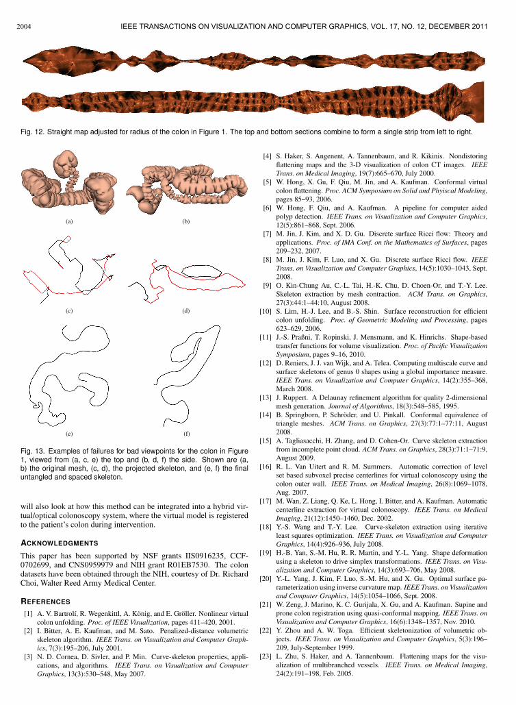
Fig. 12. Straight map adjusted for radius of the colon in Figure 1. The top and bottom sections combine to form a single strip from left to right.

(a) (b)

(c) (d)

(e) (f)

Fig. 13. Examples of failures for bad viewpoints for the colon in Figure1, viewed from (a, c, e) the top and (b, d, f) the side. Shown are (a,b) the original mesh, (c, d), the projected skeleton, and (e, f) the finaluntangled and spaced skeleton.

will also look at how this method can be integrated into a hybrid vir-tual/optical colonoscopy system, where the virtual model is registeredto the patient’s colon during intervention.

ACKNOWLEDGMENTS

This paper has been supported by NSF grants IIS0916235, CCF-0702699, and CNS0959979 and NIH grant R01EB7530. The colondatasets have been obtained through the NIH, courtesy of Dr. RichardChoi, Walter Reed Army Medical Center.

REFERENCES

[1] A. V. Bartrolı, R. Wegenkittl, A. Konig, and E. Groller. Nonlinear virtual

colon unfolding. Proc. of IEEE Visualization, pages 411–420, 2001.

[2] I. Bitter, A. E. Kaufman, and M. Sato. Penalized-distance volumetric

skeleton algorithm. IEEE Trans. on Visualization and Computer Graph-

ics, 7(3):195–206, July 2001.

[3] N. D. Cornea, D. Sivler, and P. Min. Curve-skeleton properties, appli-

cations, and algorithms. IEEE Trans. on Visualization and Computer

Graphics, 13(3):530–548, May 2007.

[4] S. Haker, S. Angenent, A. Tannenbaum, and R. Kikinis. Nondistoring

flattening maps and the 3-D visualization of colon CT images. IEEE

Trans. on Medical Imaging, 19(7):665–670, July 2000.

[5] W. Hong, X. Gu, F. Qiu, M. Jin, and A. Kaufman. Conformal virtual

colon flattening. Proc. ACM Symposium on Solid and Phyiscal Modeling,

pages 85–93, 2006.

[6] W. Hong, F. Qiu, and A. Kaufman. A pipeline for computer aided

polyp detection. IEEE Trans. on Visualization and Computer Graphics,

12(5):861–868, Sept. 2006.

[7] M. Jin, J. Kim, and X. D. Gu. Discrete surface Ricci flow: Theory and

applications. Proc. of IMA Conf. on the Mathematics of Surfaces, pages

209–232, 2007.

[8] M. Jin, J. Kim, F. Luo, and X. Gu. Discrete surface Ricci flow. IEEE

Trans. on Visualization and Computer Graphics, 14(5):1030–1043, Sept.

2008.

[9] O. Kin-Chung Au, C.-L. Tai, H.-K. Chu, D. Choen-Or, and T.-Y. Lee.

Skeleton extraction by mesh contraction. ACM Trans. on Graphics,

27(3):44:1–44:10, August 2008.

[10] S. Lim, H.-J. Lee, and B.-S. Shin. Surface reconstruction for efficient

colon unfolding. Proc. of Geometric Modeling and Processing, pages

623–629, 2006.

[11] J.-S. Praßni, T. Ropinski, J. Mensmann, and K. Hinrichs. Shape-based

transfer functions for volume visualization. Proc. of Pacific Visualization

Symposium, pages 9–16, 2010.

[12] D. Reniers, J. J. van Wijk, and A. Telea. Computing multiscale curve and

surface skeletons of genus 0 shapes using a global importance measure.

IEEE Trans. on Visualization and Computer Graphics, 14(2):355–368,

March 2008.

[13] J. Ruppert. A Delaunay refinement algorithm for quality 2-dimensional

mesh generation. Journal of Algorithms, 18(3):548–585, 1995.

[14] B. Springborn, P. Schroder, and U. Pinkall. Conformal equivalence of

triangle meshes. ACM Trans. on Graphics, 27(3):77:1–77:11, August

2008.

[15] A. Tagliasacchi, H. Zhang, and D. Cohen-Or. Curve skeleton extraction

from incomplete point cloud. ACM Trans. on Graphics, 28(3):71:1–71:9,

August 2009.

[16] R. L. Van Uitert and R. M. Summers. Automatic correction of level

set based subvoxel precise centerlines for virtual colonoscopy using the

colon outer wall. IEEE Trans. on Medical Imaging, 26(8):1069–1078,

Aug. 2007.

[17] M. Wan, Z. Liang, Q. Ke, L. Hong, I. Bitter, and A. Kaufman. Automatic

centerline extraction for virtual colonoscopy. IEEE Trans. on Medical

Imaging, 21(12):1450–1460, Dec. 2002.

[18] Y.-S. Wang and T.-Y. Lee. Curve-skeleton extraction using iterative

least squares optimization. IEEE Trans. on Visualization and Computer

Graphics, 14(4):926–936, July 2008.

[19] H.-B. Yan, S.-M. Hu, R. R. Martin, and Y.-L. Yang. Shape deformation

using a skeleton to drive simplex transformations. IEEE Trans. on Visu-

alization and Computer Graphics, 14(3):693–706, May 2008.

[20] Y.-L. Yang, J. Kim, F. Luo, S.-M. Hu, and X. Gu. Optimal surface pa-

rameterization using inverse curvature map. IEEE Trans. on Visualization

and Computer Graphics, 14(5):1054–1066, Sept. 2008.

[21] W. Zeng, J. Marino, K. C. Gurijala, X. Gu, and A. Kaufman. Supine and

prone colon registration using quasi-conformal mapping. IEEE Trans. on

Visualization and Computer Graphics, 16(6):1348–1357, Nov. 2010.

[22] Y. Zhou and A. W. Toga. Efficient skeletonization of volumetric ob-

jects. IEEE Trans. on Visualization and Computer Graphics, 5(3):196–

209, July-September 1999.

[23] L. Zhu, S. Haker, and A. Tannenbaum. Flattening maps for the visu-

alization of multibranched vessels. IEEE Trans. on Medical Imaging,

24(2):191–198, Feb. 2005.

2004 IEEE TRANSACTIONS ON VISUALIZATION AND COMPUTER GRAPHICS, VOL. 17, NO. 12, DECEMBER 2011