Context Encoders: Feature Learning by Inpainting

Deepak Pathak Philipp Krahenbuhl Jeff Donahue Trevor Darrell Alexei A. EfrosUniversity of California, Berkeley

{pathak,philkr,jdonahue,trevor,efros}@cs.berkeley.edu

Abstract

We present an unsupervised visual feature learning algo-rithm driven by context-based pixel prediction. By analogywith auto-encoders, we propose Context Encoders – a con-volutional neural network trained to generate the contentsof an arbitrary image region conditioned on its surround-ings. In order to succeed at this task, context encodersneed to both understand the content of the entire image,as well as produce a plausible hypothesis for the missingpart(s). When training context encoders, we have experi-mented with both a standard pixel-wise reconstruction loss,as well as a reconstruction plus an adversarial loss. Thelatter produces much sharper results because it can betterhandle multiple modes in the output. We found that a con-text encoder learns a representation that captures not justappearance but also the semantics of visual structures. Wequantitatively demonstrate the effectiveness of our learnedfeatures for CNN pre-training on classification, detection,and segmentation tasks. Furthermore, context encoders canbe used for semantic inpainting tasks, either stand-alone oras initialization for non-parametric methods.

1. IntroductionOur visual world is very diverse, yet highly structured,

and humans have an uncanny ability to make sense of thisstructure. In this work, we explore whether state-of-the-artcomputer vision algorithms can do the same. Consider theimage shown in Figure 1a. Although the center part of theimage is missing, most of us can easily imagine its contentfrom the surrounding pixels, without having ever seen thatexact scene. Some of us can even draw it, as shown on Fig-ure 1b. This ability comes from the fact that natural images,despite their diversity, are highly structured (e.g. the regularpattern of windows on the facade). We humans are able tounderstand this structure and make visual predictions evenwhen seeing only parts of the scene. In this paper, we show

The code, trained models and more inpainting results are available atthe author’s project website.

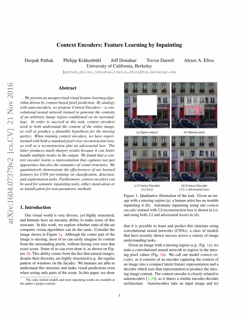
(a) Input context (b) Human artist

(c) Context Encoder(L2 loss)

(d) Context Encoder(L2 + Adversarial loss)

Figure 1: Qualitative illustration of the task. Given an im-age with a missing region (a), a human artist has no troubleinpainting it (b). Automatic inpainting using our contextencoder trained with L2 reconstruction loss is shown in (c),and using both L2 and adversarial losses in (d).

that it is possible to learn and predict this structure usingconvolutional neural networks (CNNs), a class of modelsthat have recently shown success across a variety of imageunderstanding tasks.

Given an image with a missing region (e.g., Fig. 1a), wetrain a convolutional neural network to regress to the miss-ing pixel values (Fig. 1d). We call our model context en-coder, as it consists of an encoder capturing the context ofan image into a compact latent feature representation and adecoder which uses that representation to produce the miss-ing image content. The context encoder is closely related toautoencoders [3, 20], as it shares a similar encoder-decoderarchitecture. Autoencoders take an input image and try

1

arX

iv:1

604.

0737

9v2

[cs

.CV

] 2

1 N

ov 2

016

to reconstruct it after it passes through a low-dimensional“bottleneck” layer, with the aim of obtaining a compact fea-ture representation of the scene. Unfortunately, this featurerepresentation is likely to just compresses the image contentwithout learning a semantically meaningful representation.Denoising autoencoders [38] address this issue by corrupt-ing the input image and requiring the network to undo thedamage. However, this corruption process is typically verylocalized and low-level, and does not require much seman-tic information to undo. In contrast, our context encoderneeds to solve a much harder task: to fill in large missingareas of the image, where it can’t get “hints” from nearbypixels. This requires a much deeper semantic understandingof the scene, and the ability to synthesize high-level featuresover large spatial extents. For example, in Figure 1a, an en-tire window needs to be conjured up “out of thin air.” Thisis similar in spirit to word2vec [30] which learns word rep-resentation from natural language sentences by predicting aword given its context.

Like autoencoders, context encoders are trained in acompletely unsupervised manner. Our results demonstratethat in order to succeed at this task, a model needs to bothunderstand the content of an image, as well as produce aplausible hypothesis for the missing parts. This task, how-ever, is inherently multi-modal as there are multiple waysto fill the missing region while also maintaining coherencewith the given context. We decouple this burden in our lossfunction by jointly training our context encoders to mini-mize both a reconstruction loss and an adversarial loss. Thereconstruction (L2) loss captures the overall structure of themissing region in relation to the context, while the the ad-versarial loss [16] has the effect of picking a particular modefrom the distribution. Figure 1 shows that using only the re-construction loss produces blurry results, whereas addingthe adversarial loss results in much sharper predictions.

We evaluate the encoder and the decoder independently.On the encoder side, we show that encoding just the con-text of an image patch and using the resulting feature toretrieve nearest neighbor contexts from a dataset producespatches which are semantically similar to the original (un-seen) patch. We further validate the quality of the learnedfeature representation by fine-tuning the encoder for a va-riety of image understanding tasks, including classifica-tion, object detection, and semantic segmentation. Weare competitive with the state-of-the-art unsupervised/self-supervised methods on those tasks. On the decoder side, weshow that our method is often able to fill in realistic imagecontent. Indeed, to the best of our knowledge, ours is thefirst parametric inpainting algorithm that is able to give rea-sonable results for semantic hole-filling (i.e. large missingregions). The context encoder can also be useful as a bet-ter visual feature for computing nearest neighbors in non-parametric inpainting methods.

2. Related work

Computer vision has made tremendous progress on se-mantic image understanding tasks such as classification, ob-ject detection, and segmentation in the past decade. Re-cently, Convolutional Neural Networks (CNNs) [13, 27]have greatly advanced the performance in these tasks [15,26,28]. The success of such models on image classificationpaved the way to tackle harder problems, including unsu-pervised understanding and generation of natural images.We briefly review the related work in each of the sub-fieldspertaining to this paper.

Unsupervised learning CNNs trained for ImageNet [37]classification with over a million labeled examples learnfeatures which generalize very well across tasks [9]. How-ever, whether such semantically informative and gener-alizable features can be learned from raw images alone,without any labels, remains an open question. Some ofthe earliest work in deep unsupervised learning are au-toencoders [3, 20]. Along similar lines, denoising autoen-coders [38] reconstruct the image from local corruptions, tomake encoding robust to such corruptions. While contextencoders could be thought of as a variant of denoising au-toencoders, the corruption applied to the model’s input isspatially much larger, requiring more semantic informationto undo.

Weakly-supervised and self-supervised learning Veryrecently, there has been significant interest in learningmeaningful representations using weakly-supervised andself-supervised learning. One useful source of supervisionis to use the temporal information contained in videos. Con-sistency across temporal frames has been used as supervi-sion to learn embeddings which perform well on a num-ber of tasks [17, 34]. Another way to use consistency is totrack patches in frames of video containing task-relevant at-tributes and use the coherence of tracked patches to guidethe training [39]. Ego-motion read off from non-vision sen-sors has been used as supervisory signal to train visual fea-tures et al. [1, 21].

Most closely related to the present paper are efforts atexploiting spatial context as a source of free and plentifulsupervisory signal. Visual Memex [29] used context to non-parametrically model object relations and to predict maskedobjects in scenes, while [6] used context to establish cor-respondences for unsupervised object discovery. However,both approaches relied on hand-designed features and didnot perform any representation learning. Recently, Doer-sch et al. [7] used the task of predicting the relative positionsof neighboring patches within an image as a way to trainan unsupervised deep feature representations. We share thesame high-level goals with Doersch et al. but fundamentally

differ in the approach: whereas [7] are solving a discrimina-tive task (is patch A above patch B or below?), our contextencoder solves a pure prediction problem (what pixel inten-sities should go in the hole?). Interestingly, similar distinc-tion exist in using language context to learn word embed-dings: Collobert and Weston [5] advocate a discriminativeapproach, whereas word2vec [30] formulate it as word pre-diction. One important benefit of our approach is that oursupervisory signal is much richer: a context encoder needsto predict roughly 15,000 real values per training example,compared to just 1 option among 8 choices in [7]. Likelydue in part to this difference, our context encoders take farless time to train than [7]. Moreover, context based predic-tion is also harder to “cheat” since low-level image features,such as chromatic aberration, do not provide any meaning-ful information, in contrast to [7] where chromatic aberra-tion partially solves the task. On the other hand, it is not yetclear if requiring faithful pixel generation is necessary forlearning good visual features.

Image generation Generative models of natural imageshave enjoyed significant research interest [16, 24, 35]. Re-cently, Radford et al. [33] proposed new convolutional ar-chitectures and optimization hyperparameters for Genera-tive Adversarial Networks (GAN) [16] producing encour-aging results. We train our context encoders using an ad-versary jointly with reconstruction loss for generating in-painting results. We discuss this in detail in Section 3.2.

Dosovitskiy et al. [10] and Rifai et al. [36] demonstratethat CNNs can learn to generate novel images of particularobject categories (chairs and faces, respectively), but rely onlarge labeled datasets with examples of these categories. Incontrast, context encoders can be applied to any unlabeledimage database and learn to generate images based on thesurrounding context.

Inpainting and hole-filling It is important to point outthat our hole-filling task cannot be handled by classical in-painting [4, 32] or texture synthesis [2, 11] approaches,since the missing region is too large for local non-semanticmethods to work well. In computer graphics, filling in largeholes is typically done via scene completion [19], involv-ing a cut-paste formulation using nearest neighbors from adataset of millions of images. However, scene completionis meant for filling in holes left by removing whole objects,and it struggles to fill arbitrary holes, e.g. amodal comple-tion of partially occluded objects. Furthermore, previouscompletion relies on a hand-crafted distance metric, such asGist [31] for nearest-neighbor computation which is infe-rior to a learned distance metric. We show that our methodis often able to inpaint semantically meaningful content ina parametric fashion, as well as provide a better feature fornearest neighbor-based inpainting methods.

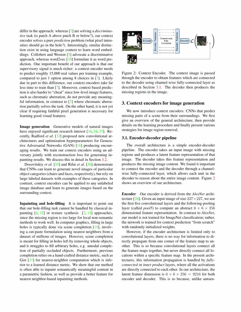
Figure 2: Context Encoder. The context image is passedthrough the encoder to obtain features which are connectedto the decoder using channel-wise fully-connected layer asdescribed in Section 3.1. The decoder then produces themissing regions in the image.

3. Context encoders for image generationWe now introduce context encoders: CNNs that predict

missing parts of a scene from their surroundings. We firstgive an overview of the general architecture, then providedetails on the learning procedure and finally present variousstrategies for image region removal.

3.1. Encoder-decoder pipeline

The overall architecture is a simple encoder-decoderpipeline. The encoder takes an input image with missingregions and produces a latent feature representation of thatimage. The decoder takes this feature representation andproduces the missing image content. We found it importantto connect the encoder and the decoder through a channel-wise fully-connected layer, which allows each unit in thedecoder to reason about the entire image content. Figure 2shows an overview of our architecture.

Encoder Our encoder is derived from the AlexNet archi-tecture [26]. Given an input image of size 227×227, we usethe first five convolutional layers and the following poolinglayer (called pool5) to compute an abstract 6 × 6 × 256dimensional feature representation. In contrast to AlexNet,our model is not trained for ImageNet classification; rather,the network is trained for context prediction “from scratch”with randomly initialized weights.

However, if the encoder architecture is limited only toconvolutional layers, there is no way for information to di-rectly propagate from one corner of the feature map to an-other. This is so because convolutional layers connect allthe feature maps together, but never directly connect all lo-cations within a specific feature map. In the present archi-tectures, this information propagation is handled by fully-connected or inner product layers, where all the activationsare directly connected to each other. In our architecture, thelatent feature dimension is 6 × 6 × 256 = 9216 for bothencoder and decoder. This is so because, unlike autoen-

coders, we do not reconstruct the original input and henceneed not have a smaller bottleneck. However, fully connect-ing the encoder and decoder would result in an explosion inthe number of parameters (over 100M!), to the extent thatefficient training on current GPUs would be difficult. Toalleviate this issue, we use a channel-wise fully-connectedlayer to connect the encoder features to the decoder, de-scribed in detail below.

Channel-wise fully-connected layer This layer is essen-tially a fully-connected layer with groups, intended to prop-agate information within activations of each feature map. Ifthe input layer has m feature maps of size n× n, this layerwill output m feature maps of dimension n × n. However,unlike a fully-connected layer, it has no parameters connect-ing different feature maps and only propagates informationwithin feature maps. Thus, the number of parameters inthis channel-wise fully-connected layer is mn4, comparedtom2n4 parameters in a fully-connected layer (ignoring thebias term). This is followed by a stride 1 convolution topropagate information across channels.

Decoder We now discuss the second half of our pipeline,the decoder, which generates pixels of the image usingthe encoder features. The “encoder features” are con-nected to the “decoder features” using a channel-wise fully-connected layer.

The channel-wise fully-connected layer is followed bya series of five up-convolutional layers [10, 28, 40] withlearned filters, each with a rectified linear unit (ReLU) acti-vation function. A up-convolutional is simply a convolutionthat results in a higher resolution image. It can be under-stood as upsampling followed by convolution (as describedin [10]), or convolution with fractional stride (as describedin [28]). The intuition behind this is straightforward – theseries of up-convolutions and non-linearities comprises anon-linear weighted upsampling of the feature produced bythe encoder until we roughly reach the original target size.

3.2. Loss function

We train our context encoders by regressing to theground truth content of the missing (dropped out) region.However, there are often multiple equally plausible ways tofill a missing image region which are consistent with thecontext. We model this behavior by having a decoupledjoint loss function to handle both continuity within the con-text and multiple modes in the output. The reconstruction(L2) loss is responsible for capturing the overall structure ofthe missing region and coherence with regards to its context,but tends to average together the multiple modes in predic-tions. The adversarial loss [16], on the other hand, triesto make prediction look real, and has the effect of picking aparticular mode from the distribution. For each ground truth

(a) Central region (b) Random block (c) Random region

Figure 3: An example of image x with our different regionmasks M applied, as described in Section 3.3.

image x, our context encoder F produces an output F (x).Let M be a binary mask corresponding to the dropped im-age region with a value of 1 wherever a pixel was droppedand 0 for input pixels. During training, those masks are au-tomatically generated for each image and training iterations,as described in Section 3.3. We now describe different com-ponents of our loss function.

Reconstruction Loss We use a normalized masked L2distance as our reconstruction loss function, Lrec,

Lrec(x) = ‖M � (x− F ((1− M)� x))‖22, (1)

where � is the element-wise product operation. We experi-mented with both L1 and L2 losses and found no significantdifference between them. While this simple loss encour-ages the decoder to produce a rough outline of the predictedobject, it often fails to capture any high frequency detail(see Fig. 1c). This stems from the fact that the L2 (or L1)loss often prefer a blurry solution, over highly accurate tex-tures. We believe this happens because it is much “safer”for the L2 loss to predict the mean of the distribution, be-cause this minimizes the mean pixel-wise error, but resultsin a blurry averaged image. We alleviated this problem byadding an adversarial loss.

Adversarial Loss Our adversarial loss is based on Gener-ative Adversarial Networks (GAN) [16]. To learn a genera-tive modelG of a data distribution, GAN proposes to jointlylearn an adversarial discriminative model D to provide lossgradients to the generative model. G and D are paramet-ric functions (e.g., deep networks) where G : Z → Xmaps samples from noise distribution Z to data distributionX . The learning procedure is a two-player game where anadversarial discriminator D takes in both the prediction ofG and ground truth samples, and tries to distinguish them,while G tries to confuse D by producing samples that ap-pear as “real” as possible. The objective for discriminator islogistic likelihood indicating whether the input is real sam-

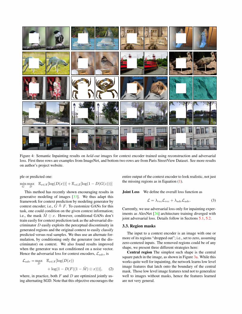
Figure 4: Semantic Inpainting results on held-out images for context encoder trained using reconstruction and adversarialloss. First three rows are examples from ImageNet, and bottom two rows are from Paris StreetView Dataset. See more resultson author’s project website.

ple or predicted one:

minG

maxD

Ex∈X [log(D(x))] + Ez∈Z [log(1−D(G(z)))]

This method has recently shown encouraging results ingenerative modeling of images [33]. We thus adapt thisframework for context prediction by modeling generator bycontext encoder; i.e., G , F . To customize GANs for thistask, one could condition on the given context information;i.e., the mask M � x. However, conditional GANs don’ttrain easily for context prediction task as the adversarial dis-criminator D easily exploits the perceptual discontinuity ingenerated regions and the original context to easily classifypredicted versus real samples. We thus use an alternate for-mulation, by conditioning only the generator (not the dis-criminator) on context. We also found results improvedwhen the generator was not conditioned on a noise vector.Hence the adversarial loss for context encoders, Ladv , is

Ladv =maxD

Ex∈X [log(D(x))

+ log(1−D(F ((1− M)� x)))], (2)

where, in practice, both F and D are optimized jointly us-ing alternating SGD. Note that this objective encourages the

entire output of the context encoder to look realistic, not justthe missing regions as in Equation (1).

Joint Loss We define the overall loss function as

L = λrecLrec + λadvLadv. (3)

Currently, we use adversarial loss only for inpainting exper-iments as AlexNet [26] architecture training diverged withjoint adversarial loss. Details follow in Sections 5.1, 5.2.

3.3. Region masks

The input to a context encoder is an image with one ormore of its regions “dropped out”; i.e., set to zero, assumingzero-centered inputs. The removed regions could be of anyshape, we present three different strategies here:

Central region The simplest such shape is the centralsquare patch in the image, as shown in Figure 3a. While thisworks quite well for inpainting, the network learns low levelimage features that latch onto the boundary of the centralmask. Those low level image features tend not to generalizewell to images without masks, hence the features learnedare not very general.

Input Context Context Encoder Content-Aware Fill

Figure 5: Comparison with Content-Aware Fill (Photoshopfeature based on [2]) on held-out images. Our methodworks better in semantic cases (top row) and works slightlyworse in textured settings (bottom row).

Random block To prevent the network from latching onthe the constant boundary of the masked region, we ran-domize the masking process. Instead of choosing a sin-gle large mask at a fixed location, we remove a number ofsmaller possibly overlapping masks, covering up to 1

4 of theimage. An example of this is shown in Figure 3b. How-ever, the random block masking still has sharp boundariesconvolutional features could latch onto.

Random region To completely remove those bound-aries, we experimented with removing arbitrary shapesfrom images, obtained from random masks in the PASCALVOC 2012 dataset [12]. We deform those shapes and pastein arbitrary places in the other images (not from PASCAL),again covering up to 1

4 of the image. Note that we com-pletely randomize the region masking process, and do notexpect or want any correlation between the source segmen-tation mask and the image. We merely use those regions toprevent the network from learning low-level features corre-sponding to the removed mask. See example in Figure 3c.

In practice, we found region and random block masksproduce a similarly general feature, while significantly out-performing the central region features. We use the randomregion dropout for all our feature based experiments.

4. Implementation detailsThe pipeline was implemented in Caffe [22] and Torch.

We used the recently proposed stochastic gradient descentsolver, ADAM [23] for optimization. The missing region inthe masked input image is filled with constant mean value.Hyper-parameter details are discussed in Sections 5.1, 5.2.

Pool-free encoders We experimented with replacing allpooling layers with convolutions of the same kernel sizeand stride. The overall stride of the network remains thesame, but it results in finer inpainting. Intuitively, there isno reason to use pooling for reconstruction based networks.

Method Mean L1 Loss Mean L2 Loss PSNR (higher better)

NN-inpainting (HOG features) 19.92% 6.92% 12.79 dB

NN-inpainting (our features) 15.10% 4.30% 14.70 dBOur Reconstruction (joint) 09.37% 1.96% 18.58 dB

Table 1: Semantic Inpainting accuracy for Paris StreetViewdataset on held-out images. NN inpainting is basis for [19].

In classification, pooling provides spatial invariance, whichmay be detrimental for reconstruction-based training. To beconsistent with prior work, we still use the original AlexNetarchitecture (with pooling) for all feature learning results.

5. Evaluation

We now evaluate the encoder features for their seman-tic quality and transferability to other image understandingtasks. We experiment with images from two datasets: ParisStreetView [8] and ImageNet [37] without using any of theaccompanying labels. In Section 5.1, we present visualiza-tions demonstrating the ability of the context encoder to fillin semantic details of images with missing regions. In Sec-tion 5.2, we demonstrate the transferability of our learnedfeatures to other tasks, using context encoders as a pre-training step for image classification, object detection, andsemantic segmentation. We compare our results on thesetasks with those of other unsupervised or self-supervisedmethods, demonstrating that our approach outperforms pre-vious methods.

5.1. Semantic Inpainting

We train context encoders with the joint loss function de-fined in Equation (3) for the task of inpainting the missingregion. The encoder and discriminator architecture is simi-lar to that of discriminator in [33], and decoder is similar togenerator in [33]. However, the bottleneck is of 4000 units(in contrast to 100 in [33]); see supplementary material. Weused the default solver hyper-parameters suggested in [33].We use λrec = 0.999 and λadv = 0.001. However, a fewthings were crucial for training the model. We did not con-dition the adversarial loss (see Section 3.2) nor did we addnoise to the encoder. We use a higher learning rate for con-text encoder (10 times) to that of adversarial discriminator.To further emphasize the consistency of prediction with thecontext, we predict a slightly larger patch that overlaps withthe context (by 7px). During training, we use higher weight(10×) for the reconstruction loss in this overlapping region.

The qualitative results are shown in Figure 4. Our modelperforms generally well in inpainting semantic regions ofan image. However, if a region can be filled with low-level textures, texture synthesis methods, such as [2, 11],can often perform better (e.g. Figure 5). For semantic in-painting, we compare against nearest neighbor inpainting(which forms the basis of Hays et al. [19]) and show that

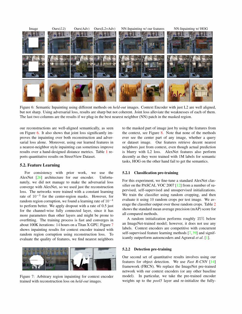
Image Ours(L2) Ours(Adv) Ours(L2+Adv) NN-Inpainting w/ our features NN-Inpainting w/ HOG

Figure 6: Semantic Inpainting using different methods on held-out images. Context Encoder with just L2 are well aligned,but not sharp. Using adversarial loss, results are sharp but not coherent. Joint loss alleviate the weaknesses of each of them.The last two columns are the results if we plug-in the best nearest neighbor (NN) patch in the masked region.

our reconstructions are well-aligned semantically, as seenon Figure 6. It also shows that joint loss significantly im-proves the inpainting over both reconstruction and adver-sarial loss alone. Moreover, using our learned features ina nearest-neighbor style inpainting can sometimes improveresults over a hand-designed distance metrics. Table 1 re-ports quantitative results on StreetView Dataset.

5.2. Feature Learning

For consistency with prior work, we use theAlexNet [26] architecture for our encoder. Unfortu-nately, we did not manage to make the adversarial lossconverge with AlexNet, so we used just the reconstructionloss. The networks were trained with a constant learningrate of 10−3 for the center-region masks. However, forrandom region corruption, we found a learning rate of 10−4

to perform better. We apply dropout with a rate of 0.5 justfor the channel-wise fully connected layer, since it hasmore parameters than other layers and might be prone tooverfitting. The training process is fast and converges inabout 100K iterations: 14 hours on a Titan X GPU. Figure 7shows inpainting results for context encoder trained withrandom region corruption using reconstruction loss. Toevaluate the quality of features, we find nearest neighbors

Figure 7: Arbitrary region inpainting for context encodertrained with reconstruction loss on held-out images.

to the masked part of image just by using the features fromthe context, see Figure 8. Note that none of the methodsever see the center part of any image, whether a queryor dataset image. Our features retrieve decent nearestneighbors just from context, even though actual predictionis blurry with L2 loss. AlexNet features also performdecently as they were trained with 1M labels for semantictasks, HOG on the other hand fail to get the semantics.

5.2.1 Classification pre-training

For this experiment, we fine-tune a standard AlexNet clas-sifier on the PASCAL VOC 2007 [12] from a number of su-pervised, self-supervised and unsupervised initializations.We train the classifier using random cropping, and thenevaluate it using 10 random crops per test image. We av-erage the classifier output over those random crops. Table 2shows the standard mean average precision (mAP) score forall compared methods.

A random initialization performs roughly 25% belowan ImageNet-trained model; however, it does not use anylabels. Context encoders are competitive with concurrentself-supervised feature learning methods [7, 39] and signif-icantly outperform autoencoders and Agrawal et al. [1].

5.2.2 Detection pre-training

Our second set of quantitative results involves using ourfeatures for object detection. We use Fast R-CNN [14]framework (FRCN). We replace the ImageNet pre-trainednetwork with our context encoders (or any other baselinemodel). In particular, we take the pre-trained encoderweights up to the pool5 layer and re-initialize the fully-

Our

s

Our

s

HO

G

HO

G

Ale

xNet

Ale

xNet

Figure 8: Context Nearest Neighbors. Center patches whose context (not shown here) are close in the embedding spaceof different methods (namely our context encoder, HOG and AlexNet). Note that the appearance of these center patchesthemselves was never seen by these methods. But our method brings them close just from their context.

Pretraining Method Supervision Pretraining time Classification Detection Segmentation

ImageNet [26] 1000 class labels 3 days 78.2% 56.8% 48.0%

Random Gaussian initialization < 1 minute 53.3% 43.4% 19.8%Autoencoder - 14 hours 53.8% 41.9% 25.2%Agrawal et al. [1] egomotion 10 hours 52.9% 41.8% -Wang et al. [39] motion 1 week 58.7% 47.4% -Doersch et al. [7] relative context 4 weeks 55.3% 46.6% -

Ours context 14 hours 56.5% 44.5% 30.0%

Table 2: Quantitative comparison for classification, detection and semantic segmentation. Classification and Fast-RCNNDetection results are on the PASCAL VOC 2007 test set. Semantic segmentation results are on the PASCAL VOC 2012validation set from the FCN evaluation described in Section 5.2.3, using the additional training data from [18], and removingoverlapping images from the validation set [28].

connected layers. We then follow the training and evalu-ation procedures from FRCN and report the accuracy (inmAP) of the resulting detector.

Our results on the test set of the PASCAL VOC 2007 [12]detection challenge are reported in Table 2. Context en-coder pre-training is competitive with the existing meth-ods achieving significant boost over the baseline. Recently,Krahenbuhl et al. [25] proposed a data-dependent methodfor rescaling pre-trained model weights. This significantlyimproves the features in Doersch et al. [7] up to 65.3%for classification and 51.1% for detection. However, thisrescaling doesn’t improve results for other methods, includ-ing ours.

5.2.3 Semantic Segmentation pre-training

Our last quantitative evaluation explores the utility of con-text encoder training for pixel-wise semantic segmentation.Fully convolutional networks [28] (FCNs) were proposed asan end-to-end learnable method of predicting a semantic la-bel at each pixel of an image, using a convolutional networkpre-trained for ImageNet classification. We replace the clas-sification pre-trained network used in the FCN method with

our context encoders, afterwards following the FCN train-ing and evaluation procedure for direct comparison withtheir original CaffeNet-based result.

Our results on the PASCAL VOC 2012 [12] validationset are reported in Table 2. In this setting, we outperform arandomly initialized network as well as a plain autoencoderwhich is trained simply to reconstruct its full input.

6. ConclusionOur context encoders trained to generate images condi-

tioned on context advance the state of the art in semanticinpainting, at the same time learn feature representationsthat are competitive with other models trained with auxil-iary supervision.

Acknowledgements The authors would like to thankAmanda Buster for the artwork on Fig. 1b, as well as Shub-ham Tulsiani and Saurabh Gupta for helpful discussions.This work was supported in part by DARPA, AFRL, In-tel, DoD MURI award N000141110688, NSF awards IIS-1212798, IIS-1427425, and IIS-1536003, the Berkeley Vi-sion and Learning Center and Berkeley Deep Drive.

References[1] P. Agrawal, J. Carreira, and J. Malik. Learning to see by

moving. ICCV, 2015. 2, 7, 8[2] C. Barnes, E. Shechtman, A. Finkelstein, and D. Goldman.

Patchmatch: A randomized correspondence algorithm forstructural image editing. ACM Transactions on Graphics,2009. 3, 6

[3] Y. Bengio. Learning deep architectures for ai. Foundationsand trends in Machine Learning, 2009. 1, 2

[4] M. Bertalmio, G. Sapiro, V. Caselles, and C. Ballester. Imageinpainting. In Computer graphics and interactive techniques,2000. 3

[5] R. Collobert and J. Weston. A unified architecture for naturallanguage processing: Deep neural networks with multitasklearning. In ICML, 2008. 3

[6] C. Doersch, A. Gupta, and A. A. Efros. Context as supervi-sory signal: Discovering objects with predictable context. InECCV, 2014. 2

[7] C. Doersch, A. Gupta, and A. A. Efros. Unsupervised visualrepresentation learning by context prediction. ICCV, 2015.2, 3, 7, 8

[8] C. Doersch, S. Singh, A. Gupta, J. Sivic, and A. Efros. Whatmakes paris look like paris? ACM Transactions on Graphics,2012. 6

[9] J. Donahue, Y. Jia, O. Vinyals, J. Hoffman, N. Zhang,E. Tzeng, and T. Darrell. Decaf: A deep convolutional ac-tivation feature for generic visual recognition. ICML, 2014.2

[10] A. Dosovitskiy, J. T. Springenberg, and T. Brox. Learning togenerate chairs with convolutional neural networks. CVPR,2015. 3, 4

[11] A. Efros and T. K. Leung. Texture synthesis by non-parametric sampling. In ICCV, 1999. 3, 6

[12] M. Everingham, S. A. Eslami, L. Van Gool, C. K. Williams,J. Winn, and A. Zisserman. The Pascal Visual Object Classeschallenge: A retrospective. IJCV, 2014. 6, 7, 8

[13] K. Fukushima. Neocognitron: A self-organizing neural net-work model for a mechanism of pattern recognition unaf-fected by shift in position. Biological cybernetics, 1980. 2

[14] R. Girshick. Fast r-cnn. ICCV, 2015. 7[15] R. Girshick, J. Donahue, T. Darrell, and J. Malik. Rich fea-

ture hierarchies for accurate object detection and semanticsegmentation. In CVPR, 2014. 2

[16] I. Goodfellow, J. Pouget-Abadie, M. Mirza, B. Xu,D. Warde-Farley, S. Ozair, A. Courville, and Y. Bengio. Gen-erative adversarial nets. In NIPS, 2014. 2, 3, 4

[17] R. Goroshin, J. Bruna, J. Tompson, D. Eigen, and Y. LeCun.Unsupervised learning of spatiotemporally coherent metrics.ICCV, 2015. 2

[18] B. Hariharan, P. Arbelaez, L. Bourdev, S. Maji, and J. Malik.Semantic contours from inverse detectors. In ICCV, 2011. 8

[19] J. Hays and A. A. Efros. Scene completion using millions ofphotographs. SIGGRAPH, 2007. 3, 6

[20] G. E. Hinton and R. R. Salakhutdinov. Reducing the dimen-sionality of data with neural networks. Science, 2006. 1,2

[21] D. Jayaraman and K. Grauman. Learning image representa-tions tied to ego-motion. In ICCV, 2015. 2

[22] Y. Jia, E. Shelhamer, J. Donahue, S. Karayev, J. Long, R. B.Girshick, S. Guadarrama, and T. Darrell. Caffe: Convolu-tional architecture for fast feature embedding. In ACM Mul-timedia, 2014. 6

[23] D. Kingma and J. Ba. Adam: A method for stochastic opti-mization. ICLR, 2015. 6

[24] D. P. Kingma and M. Welling. Auto-encoding variationalbayes. ICLR, 2014. 3

[25] P. Krahenbuhl, C. Doersch, J. Donahue, and T. Darrell. Data-dependent initializations of convolutional neural networks.ICLR, 2016. 8

[26] A. Krizhevsky, I. Sutskever, and G. E. Hinton. ImageNetclassification with deep convolutional neural networks. InNIPS, 2012. 2, 3, 5, 7, 8, 10

[27] Y. LeCun, B. Boser, J. S. Denker, D. Henderson, R. E.Howard, W. Hubbard, and L. D. Jackel. Backpropagationapplied to handwritten zip code recognition. Neural compu-tation, 1989. 2

[28] J. Long, E. Shelhamer, and T. Darrell. Fully convolutionalnetworks for semantic segmentation. In CVPR, 2015. 2, 4, 8

[29] T. Malisiewicz and A. Efros. Beyond categories: The visualmemex model for reasoning about object relationships. InNIPS, 2009. 2

[30] T. Mikolov, I. Sutskever, K. Chen, G. S. Corrado, andJ. Dean. Distributed representations of words and phrasesand their compositionality. In NIPS, 2013. 2, 3

[31] A. Oliva and A. Torralba. Building the gist of a scene: Therole of global image features in recognition. Progress inbrain research, 2006. 3

[32] S. Osher, M. Burger, D. Goldfarb, J. Xu, and W. Yin. An it-erative regularization method for total variation-based imagerestoration. Multiscale Modeling & Simulation, 2005. 3

[33] A. Radford, L. Metz, and S. Chintala. Unsupervised repre-sentation learning with deep convolutional generative adver-sarial networks. ICLR, 2016. 3, 5, 6, 10

[34] V. Ramanathan, K. Tang, G. Mori, and L. Fei-Fei. Learn-ing temporal embeddings for complex video analysis. ICCV,2015. 2

[35] M. Ranzato, V. Mnih, J. M. Susskind, and G. E. Hinton.Modeling natural images using gated mrfs. PAMI, 2013. 3

[36] S. Rifai, Y. Bengio, A. Courville, P. Vincent, and M. Mirza.Disentangling factors of variation for facial expressionrecognition. In ECCV, 2012. 3

[37] O. Russakovsky, J. Deng, H. Su, J. Krause, S. Satheesh,S. Ma, Z. Huang, A. Karpathy, A. Khosla, M. Bernstein,A. C. Berg, and L. Fei-Fei. Imagenet large scale visual recog-nition challenge. IJCV, 2015. 2, 6

[38] P. Vincent, H. Larochelle, Y. Bengio, and P.-A. Manzagol.Extracting and composing robust features with denoising au-toencoders. In ICML, 2008. 2

[39] X. Wang and A. Gupta. Unsupervised learning of visual rep-resentations using videos. ICCV, 2015. 2, 7, 8

[40] M. D. Zeiler and R. Fergus. Visualizing and understandingconvolutional networks. In ECCV, 2014. 4

Supplementary MaterialIn this section, we present the architectural details of our

context-encoders, and show additional qualitative results.Context encoders are not only able to inpaint semantic de-tails in the missing part of an input image, but also learnfeatures transferable to other tasks. We discuss the imple-mentation details for each of these in following sections.

A. Semantic Inpainting

Context encoders for inpainting are trained jointly withreconstruction and adversarial loss as discussed in Sec-tion 5.1. The inpainting results are slightly worse if we use227 × 227 directly. So, we resize images to 128 × 128and then train our joint loss with the resized images. Theencoder and discriminator architecture is similar to that ofdiscriminator in [33], and decoder is similar to generatorin [33]; the bottleneck is of 4000 units. We used batchnormalization in both context encoder and discriminator.ReLU [26] non-linearity is used in decoder, while leakyReLU [33] is used in both encoder and discriminator.

In case of arbitrary region inpainting, adversarial dis-criminator compares the full real image and the full gen-erated image. We do not condition the adversarial discrimi-nator with mask, see (2). If the discriminator sees the mask,it figures out the perceptual discontinuity of generated partfrom the real part and easily classifies the real v/s the gen-erated image, i.e., the process doesn’t train. Moreover, par-ticularly for center region inpainting, this process can becomputationally simplified by producing center only andnot showing discriminator the context boundary (or in otherwords, not showing the mask). The exact architecture forcenter region dropout is shown in Figure 9a.

B. Feature Learning

We use the AlexNet [26] architecture for encoder so thatwe can compare the learned features with the prior works,which are trained using Imagenet labels and other un/self-supervised techniques. The encoder is Alexnet until pool5,followed by channel-wise fully connected layer and decoderis a series of upconvolutional layers until we reach the tar-get size. The input image size is 227× 227. Unfortunately,we couldn’t train adversary with Alexnet Encoder, so it istrained with reconstruction loss. See Figure 9b for exactarchitecture details. For pre-training experiments in Sec-tion 5.2, we randomly initialize the fully-connected lay-ers, i.e., fc6 and fc7, while starting from context encoderweights.

C. Additional Results

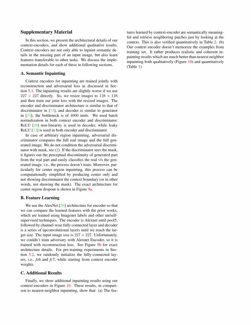
Finally, we show additional inpainting results using ourcontext-encoders in Figure 10. These results, in compari-son to nearest-neighbor inpainting, show that: (a) The fea-

tures learned by context-encoder are semantically meaning-ful and retrieve neighboring patches just by looking at thecontext. This is also verified quantitatively in Table 2. (b)Our context encoder doesn’t memorize the examples fromtraining set. It rather produces realistic and coherent in-painting results which are much better than nearest neighborinpainting both qualitatively (Figure 10) and quantitatively(Table 1).

Reconstruc*onLoss(L2)

64

64

64

32

32 64128

256 512

16 8 4

8 4

4000

4x4(conv)

4x4(conv)

4x4(conv)

4x4(conv)

4x4(conv)

512

4

4

4x4(uconv)

256

8

8

4x4(uconv)

128

16

4x4(uconv)

32

32

4x4(uconv)

4x4(uconv)

64

64

64

4x4(conv)

1616

32

32 64128

256 512

16 8 4

8 4

4x4(conv)

4x4(conv)

4x4(conv)

4x4(conv)

4x4(conv)

16

64

64

128

128

realorfake

Encoder Decoder

AdversarialDiscriminator

(a) Context encoder trained with joint reconstruction and adversarial loss for semantic inpainting. This illustration is shown for center region dropout.Similar architecture holds for arbitrary region dropout as well. See Section 3.2.

Reconstruc*onLoss(L2)

9216

256

6

6

(reshape)

128

11

11

5x5(uconv)

64

21

5x5(uconv)

41

41

5x5(uconv)

5x5(uconv)

32

21

227

227

Encoder Decoder

AlexNet(un*lpool5)

64

81

81

5x5(uconv)

3161

161 227

227

9216

(resize)

Channel-wiseFully

Connected

(b) Context encoder trained with reconstruction loss for feature learning by filling in arbitrary region dropouts in the input.

Figure 9: Context encoder training architectures.

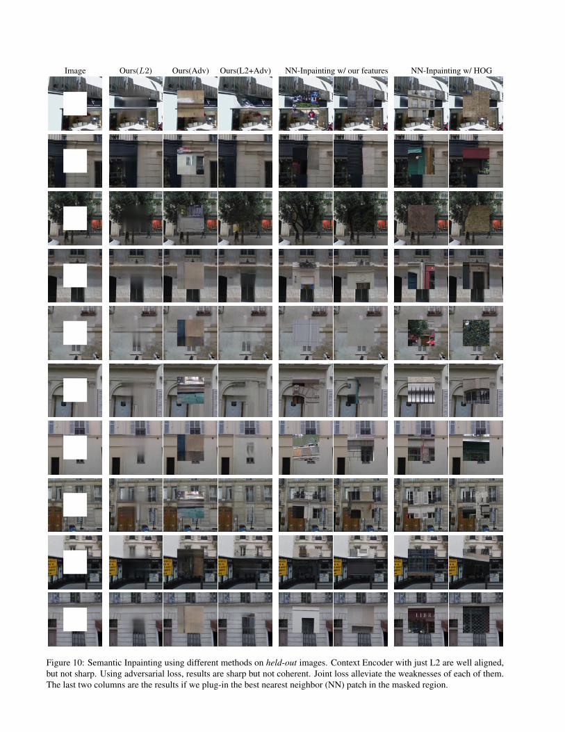
Image Ours(L2) Ours(Adv) Ours(L2+Adv) NN-Inpainting w/ our features NN-Inpainting w/ HOG

Figure 10: Semantic Inpainting using different methods on held-out images. Context Encoder with just L2 are well aligned,but not sharp. Using adversarial loss, results are sharp but not coherent. Joint loss alleviate the weaknesses of each of them.The last two columns are the results if we plug-in the best nearest neighbor (NN) patch in the masked region.

Figure 10: Semantic Inpainting using different methods on held-out images. Context Encoder with just L2 are well aligned,but not sharp. Using adversarial loss, results are sharp but not coherent. Joint loss alleviate the weaknesses of each of them.The last two columns are the results if we plug-in the best nearest neighbor (NN) patch in the masked region.