Context-Based Pedestrian Path Prediction - Gavrila · Context-Based Pedestrian Path Prediction Julian Francisco Pieter Kooij 1,2, ... goes beyond the state-of-the-art on pedestrian

Context-Based Pedestrian Path Prediction�

Julian Francisco Pieter Kooij1,2, Nicolas Schneider1,2,Fabian Flohr1,2, and Dariu M. Gavrila1,2

1 Environment Perception, Daimler R&D, Ulm, Germany{nicolas.schneider,fabian.flohr}@daimler.com

2 Intelligent Systems Laboratory, Univ. of Amsterdam, The Netherlands{J.F.P.Kooij,D.M.Gavrila}@uva.nl

Abstract. We present a novel Dynamic Bayesian Network for pedestrian pathprediction in the intelligent vehicle domain. The model incorporates the pedes-trian situational awareness, situation criticality and spatial layout of the environ-ment as latent states on top of a Switching Linear Dynamical System (SLDS) toanticipate changes in the pedestrian dynamics. Using computer vision, situationalawareness is assessed by the pedestrian head orientation, situation criticality bythe distance between vehicle and pedestrian at the expected point of closest ap-proach, and spatial layout by the distance of the pedestrian to the curbside. Ourparticular scenario is that of a crossing pedestrian, who might stop or continuewalking at the curb. In experiments using stereo vision data obtained from a ve-hicle, we demonstrate that the proposed approach results in more accurate pathprediction than only SLDS, at the relevant short time horizon (1 s), and slightlyoutperforms a computationally more demanding state-of-the-art method.

Keywords: intelligent vehicles, path prediction, situational awareness, visual fo-cus of attention, Dynamic Bayesian Network, Linear Dynamical System.

1 Introduction

The past decade has seen a significant progress on video-based pedestrian detection. Inthe intelligent vehicle domain, this has recently culminated in the market introductionof active pedestrian systems that can perform automatic braking in case of dangeroustraffic situations. An area that holds major potential for further improvement is situa-tion assessment. Current active pedestrian systems are designed conservatively in theirwarning and control strategy, emphasizing the current pedestrian state (i.e. position)rather than prediction, in order to avoid false system activations. Indeed, pedestrian pathprediction is a challenging problem, due to the highly dynamic nature of pedestrian mo-tion, and systems need to react with limited computation time. Small deviations of, say,30 cm in the estimated lateral position of the pedestrian can make all the difference, asthis might place the pedestrian just inside or outside the driving corridor.

� Electronic supplementary material -Supplementary material is available in the online ver-sion of this chapter at http://dx.doi.org/10.1007/978-3-319-1059 - _40Videos can also be accessed at http://www.springerimages.com/videos/978-3-319-10598-7

D. Fleet et al. (Eds.): ECCV 2014, Part VI, LNCS 8694, pp. 618–633, 2014.c© Springer International Publishing Switzerland 2014

9 4

http://dx.doi.org/10.1007/978-3-319-10598-7_40

http://www.springerimages.com/videos/978-3-319-10598-7

http://www.springerimages.com/videos/978-3-319-10598-7

Context-Based Pedestrian Path Prediction 619

SC0

SV0

HSV0

M0

AC0

X0

Dmin0 HO0 Y0 DTC0

SC1

SV1

HSV1

M1

AC1

X1

Dmin1 HO1 Y1 DTC1

Fig. 1. Left: Pedestrian path prediction from an approaching vehicle, using situation criticality,pedestrian awareness thereof, and positioning vs. curbside. Right: DBN as directed graph, un-rolled for two time slices. Discrete/continuous/observed nodes are rectangular/circular/shaded.

This paper focuses on the accurate path prediction of pedestrians intending to later-ally cross the street, as observed by a stereo camera on-board an approaching vehicle(accident analysis shows that this scenario accounts for a majority of all pedestrian fatal-ities in traffic [23]). We argue that the pedestrian’s decision to stop is for a large degreeinfluenced by three factors: the existence of an approaching vehicle on collision course,the pedestrian’s awareness thereof, and the spatial layout of the environment. We there-fore propose a Dynamic Bayesian Network (DBN), which captures these factors as latentstates on top of a Switching Linear Dynamical System (SLDS), thus controlling changesin the pedestrian dynamics. We estimate situation criticality by the distance betweenvehicle and pedestrian at the expected point of closest approach. Situational awarenessassesses whether the pedestrian has seen the vehicle at some point up to now (whetherthe pedestrian currently sees the vehicle is estimated by means of the head orientation).Spatial layout is captured by the distance of the pedestrian to the road curbside. SeeFig. 1 for an illustration of the scenario. The observables (shaded nodes in the graphicalmodel), i.e. distance at closest approach, pedestrian location, head orientation, curbsidelocation, are provided by external, state-of-the-art system components, for which we donot make novelty claims.

All DBN parameters are estimated from annotated training data. In the experiments,we collected data of pedestrians crossing in a supervised setting in traffic situations,where the vehicle has an implicit right-of-way. It would be straightforward to applythe approach to traffic situations where traffic lights or pedestrian crossings changethe right-of-way, by adding an (observed) context variable to the DBN. Our approachcan also be extended to additional motion types (e.g. pedestrian crossing the road in acurved path) or, more generally, to robot navigation in human-inhabited environments.

2 Previous Work

In this section, we focus on techniques for pedestrian state estimation and path predic-tion. For vision-based pedestrian detection, see recent surveys e.g. [10,12]. For pedes-trian head/body orientation estimation, see e.g. [5,13,14].

State estimation in dynamical systems often involves the assumption that the under-lying model is linear and that the noise is Gaussian, mainly due to the availability of the

620 J.F.P. Kooij et al.

Kalman filter (KF) [7] as an efficient inference algorithm for such Linear DynamicalSystems (LDS). In the intelligent vehicle domain, the KF is the most popular choicefor pedestrian tracking (see [30] for an overview). The state distribution of a LDS canbe propagated into the future without incorporating new observations to account formissing measurements, or to perform path prediction. The Extended and Unscented KF[24] can, to a certain degree, account for non-linear dynamical or measurement models,but Switching LDS (SLDS) are needed for maneuvering targets that alternate variousmotion types. A SLDS uses a top-level discrete Markov chain to select per time stepthe system dynamics of the underlying LDS. However, exact inference and learning be-comes intractable as the number of modes in the posterior distribution grows exponen-tial over time in the number of the switching states [27]. One solution is to approximatethe posterior by samples using some Markov Chain Monte Carlo method [26,29]. Sam-pling can also be used when extending the SLDS hierarchy, e.g. to impose distributionson persistent state durations [26], or learn an SLDS mixture to cluster trajectories whichexhibit similar switching behavior [21]. However, sampling is impractical for onlinereal-time inference as convergence can be slow. Another solution is Assumed DensityFiltering (ADF) [6,25], which approximates the posterior at every time step with a sim-pler distribution. ADF can be applied to discrete state DBNs, known as Boyen-Kollerinference [8], and more generally to mixed discrete-continuous state spaces with con-ditional Gaussian posterior [22]. Interacting Multiple Model KF [7] is related to ADFfor SLDS, as it mixes the states of several KF filters running in parallel, and has beenapplied for path prediction in the intelligent vehicle domain [18,30].

Whereas SLDSs can account for changes in dynamics, a switch in dynamics will onlybe detected after sufficient observations contradict the currently predominant dynamicmodel. If we wish to anticipate instead of react to changes in dynamics, a model shouldinclude possible causes for change. These influences on pedestrian behavior can becaptured on an individual level using agent models, which have been used to reasonabout pedestrian intent [4,19] (i.e. where does observed agent want to go), account forpreferences to move around certain regions of a static scene [19], and avoid collisionwith other agents, as is done in social force models [2,16]. [32] enhanced social forcetowards group behavior by introducing sub-goals such as “following a person”. Therelated Linear Trajectory Avoidance model [28] for short-term path prediction uses theexpected point of closest approach to foreshadow and avoid possible collisions.

These agent-based models assume that pedestrians are fully aware of their environ-ment [19,28]. However, this assumption does not hold when dealing with inattentivepedestrians in the intelligent vehicle context. [15] presented a study on head turningbehaviors at pedestrian crosswalks regarding the best point of warning for inattentivepedestrians. They used gyro sensors to record head turning and let pedestrians press abutton when they recognize an approaching vehicle. Apart from this sole study of Vi-sual Focus of Attention (VFOA) in intelligent vehicle context we are aware of, VFOAhas been investigated in other application contexts. For example, [5] used a HOG-basedhead detector to determine pedestrian attention for automated surveillance, and [3] com-bined contextual cues in a DBN to model influence of group interaction on VFOA.

Within the class of non-parametric methods for path prediction and action classifi-cation, [18] recently proposed two non-linear, higher order Markov models to estimate


whether a crossing pedestrian will stop at the curbside, one using Gaussian Process Dy-namical Models (GPDM), and one using Probabilistic Hierarchical Trajectory Match-ing (PHTM). Both models use dense optical flow features in the pedestrian boundingbox, in addition to the positional information. The first approach learns a GPDM of thedense flow for walking and stopping motion to predict future flow fields (and therebylateral velocity). PHTM matches feature vectors of flow and position to a hierarchicallyorganized tracklet database to extrapolate motion. Both approaches were shown to per-form similar, and outperform the first-order Markov LDS and SLDS models, albeit at alarge computational cost ([18] reports GPDM/PHTM is three/two orders of magnitudeslower than KF). [20] considered the complementary case, whether a standing pedes-trian will start to walk at the curbside. This only involved action classification and nopath prediction, and an infrastructure-based sensor setup (no on-board vehicle sensing).

3 Proposed Approach

We are interested in modeling the motion dynamics of a pedestrian from the viewpointof an approaching vehicle, in order to perform accurate path prediction. We considerthat non-maneuvering pedestrian movement is well captured by a LDS with a basicmotion model (e.g. constant position, constant velocity, constant turn rate) [7], and thatmaneuvering pedestrian movement can be suitably represented by means of an SLDS.Thus, the switching state indicates which basic motion model to use at any moment.

In this paper, we propose to condition the transition matrix of the SLDS switchingstate on latent factors that are likely going to influence the pedestrian’s motion type.In a scenario of a lateral crossing pedestrian, we argue that the pedestrian’s decisionto continue walking or to stop is largely influenced by the existence of an approachingvehicle on collision course, the pedestrian’s awareness thereof, and the position of thepedestrian with respect to the curbside.

Hence, we consider our main paper contribution a DBN which captures these threefactors as latent states on top of an SLDS (see current section). The proposed approachgoes beyond the state-of-the-art on pedestrian path prediction in vehicle context, whichhas considered the pedestrian in isolation, i.e. context free [18,20,30], and agent modelsthat ignore a pedestrian’s perception and resulting situational awareness [4,19,28].

3.1 Graphical Model

The proposed DBN is shown in Fig. 1. We distinguish two sets of variables: thoserelating to a SLDS (consisting of switching state M , latent position state X and asso-ciated observation Y ) and those related to the scene context, i.e. spatial layout, situ-ation criticality and the pedestrian’s awareness (consisting of discrete latent variablesZ = {SV,HSV, SC,AC}) that influence the SLDS switching state, and associated ob-servables E =

{HO,Dmin, DTC

}. These variables are now discussed in turn. Details

on parameter estimation and computation of observables are given in Sec. 4.2.

SLDS. A SLDS contains a discrete switching state Mt, a continuous hidden state Xt,and a linear observation of the state Yt with noise N (0, R) added. In our application, we


consider that any moment can exhibit one of two motion types, walking (Mt = mw) andstanding (Mt = ms). While the velocity of any standing person is zero, different peoplecan have different walking velocities, i.e. some people move faster than others. Let xt

denote a person’s lateral position at time t (after vehicle ego-motion compensation) andvt the corresponding velocity. Furthermore, vmw is the personal walking velocity of thepedestrian. The motion dynamics over a period Δt can then be described as,

xt = xt−Δt + vtΔt+ εtΔt vt =

{0 iff Mt = ms

vmw iff Mt = mw(1)

Here εt ∼ N (0, Q) is zero-mean process noise that allows for deviations of the fixedvelocity assumption. We will assume fixed time-intervals, and from here on set Δt = 1.

We include the velocity vmw in the state of an SLDS, together with the position xt,such that we can filter both as we obtain observations over time, i.e. Xt = [xt, v

mwt ]�,

Xt = A(Mt)Xt−1 +

[εt0

]εt ∼ N (0, Q) (2)

Yt = CXt + ηt ηt ∼ N (0, R) (3)

where the switching state Mt selects the appropriate linear state transformation A(m),

A(ms) =

[1 00 1

]A(mw) =

[1 10 1

]. (4)

Yt ∈ R is the observed lateral position with observation matrix C = [1 0]. The ini-tial distribution on the state X0 expresses our prior beliefs about a pedestrian’s po-sition and walking speed, as learned from the training data (see Sec. 4.2). From thedefinition of the SLDS, we obtain the following conditional probability distributionsfor the graphical model, P (Xt|Xt−1,Mt) = N (Xt|A(Mt)Xt−1, Q) and P (Yt|Xt) =N (Yt|CXt, R).

Context. The transition probability of the SLDS switching state is conditioned on theBoolean latent context variables Z . Although all these variables are discrete, duringinference the uncertainty propagates from the observables to these variables (and overtime), resulting in posterior distributions that contain values between 0 and 1. Each con-textual configuration Zt = z is associated with a motion model transition probabilityPz , where P(·) indicates that the distribution is represented by a probability table, andthe subscript here denotes a table for each value z, such that

P (Mt|Mt−1, Zt = z) = Pz(Mt|Mt−1). (5)

The temporal transition of the context in Z is factorized by the probability tables

P (Zt|Zt−1) = P(HSVt|HSVt−1, SVt)× P(SVt|SVt−1)

×P(SCt|SCt−1)× P(ACt|ACt−1).(6)

The latent Sees-Vehicle (SV ) variable indicates whether the pedestrian is currentlyseeing the vehicle. Has-Seen-Vehicle (HSV ) indicates whether the pedestrian is aware


of the vehicle, i.e. whether SVt′ = true for some t′ ≤ t. The transition probability ofHSVt encodes simply a logical OR between the Boolean HSVt−1 and SVt nodes:

P(HSVt|HSVt−1, SVt) =

{1 iff HSVt = (HSVt−1 ∨ SVt)0 otherwise.

(7)

The latent variable Situation-Critical (SC) indicates whether a situation is critical whenboth, pedestrian and vehicle, continue with their current velocities. At-Curb (AC) in-dicates if the pedestrian is currently at the distance from the curbside (as found in thetraining data) where a person would stop if they choose to wait and postpone cross-ing the road. The SV , SC and AC nodes furthermore depend on their value in thepreceding time step, which improves the temporal consistency of these latent variables.

Next we discuss observations Et which provide evidence for the latent context Zt,

P (Et|Zt) = P (HOt|SVt)× P (Dmint |SCt)× P (DTC|ACt). (8)

The Head-Orientation observable HOt serves as evidence for the Sees-Vehicle (SVt)variable. We apply multiple classifiers to the head image region, each trained to detectthe head in a particular looking direction (for details, see Section 4.1), and HOt is thena vector with the classifier responses. The values in this vector form different unnor-malized distributions over the classes, depending on whether the pedestrian is lookingat the vehicle or not. However, if the head is not clearly observed (e.g. it is too far, orin the shadow), all values are typically low, and the observed class distribution provideslittle evidence of the true head orientation. We therefore model HOt as a sample froma Multinomial distribution conditioned on SVt, with parameter vector psv,

P (HOt|SVt = sv) = Mult(HOt|psv). (9)

As such, higher classifier outputs count as stronger evidence for the presence of thatclass in the observation. In the other limit of all zero outputs, HOt will have equallikelihood for any value of SVt.

For Situation-Critical (SC), we consider the minimum distance Dmin between thepedestrian and vehicle, if their paths would be extrapolated in time with fixed veloc-ity [28]. While this indicator makes naive assumptions about the vehicle and pedestrianmotion, it is still informative as a measure of how critical the situation is, and thereby,as part of our model, will lead to more accurate pedestrian path prediction. We define aGamma distribution over Dmin given SC, parametrized by shape a and scale b,

P (Dmint |SCt = sc) = Γ (Dmin

t |asc, bsc). (10)

To obtain evidence for At-Curb (ACt), we detect the curb ridge in the image, andmeasure its lateral position near the pedestrian. These noisy measurements are filteredwith a constant position Kalman filter with zero process noise, such that we obtain anaccurate estimate of the expected curb position, xcurb

t . Distance-To-Curb,DTCt, is thencalculated as the difference between the expected filtered position of the pedestrian,E[xt], and of the curb, xcurb

t . Note that for path prediction we can estimate DTC evenat future time steps, using predicted pedestrian positions, and accordingly predict ACtoo. The distribution over DTCt given AC is modeled as a Normal distribution,

P (DTCt|ACt = ac) = N (DTCt|μac, σac). (11)


3.2 Inference

The DBN is used in a forward filtering procedure to incorporate all available observa-tions of new time instances directly when they are received. We have a mixed discrete-continuous DBN where the exact posterior includes a mixture of |M |T Normal modesafter T time steps, hence exact inference is intractable. We therefore resort to AssumedDensity Filtering [22,25] for approximate inference, where after each time step thefound posterior is approximated by a simpler distribution. The procedure consists ofexecuting the following three steps for each time instance: predict, update, and collapse.

We will let P t(·) ≡ P (·|O1:t−1) denote a prediction for time t (i.e. before receivingthe observation Ot), and Pt(·) ≡ P (·|O1:t) denote an updated estimate for time t (i.e.after observing Ot). Finally, Pt(·) is the collapsed or approximated updated distributionthat will be carried over to the predict step of the next time instance t+ 1.

Predict. To predict time t we use the posterior distribution of t − 1, which is factor-ized into the joint distribution over the latent discrete nodes Pt−1(Mt−1, Zt−1) and the

conditional Normal distribution Pt−1(Xt−1|Mt−1) = N (Xt−1|μ(Mt−1)t−1 , Σ

(Mt−1)t−1 ).

First, the joint probability of the discrete nodes in the previous and current time stepsis computed using the factorized transition tables of Eq. (5) and (6),

P t(Mt,Mt−1, Zt, Zt−1) = P (Mt|Mt−1, Zt)P (Zt|Zt−1)Pt−1(Mt−1, Zt−1). (12)

Then for the continuous latent state Xt we predict the effect of the linear dynamicsof all possible models Mt on the conditional Normal distribution of each Mt−1,

P t(Xt|Mt,Mt−1) =

∫P (Xt|Xt−1,Mt)× Pt−1(Xt−1|Mt−1) dXt−1. (13)

Applying Eq. (2), we find that the parametric form of (13) is the Kalman prediction step

N (Xt|μ(Mt,Mt−1)t , Σ

(Mt,Mt−1)

t ) =∫

N (Xt|A(Mt)Xt−1, Q)×N (Xt−1|μ(Mt−1)t−1 , Σ

(Mt−1)t−1 ) dXt−1.

(14)

Update. The update step incorporates the observations of the current time step to obtainthe joint posterior. For each joint assignment (Mt,Mt−1), the LDS likelihood term is

P (Yt|Mt,Mt−1) =

∫P (Yt|Xt)× P t(Xt|Mt,Mt−1) dXt

= N (Yt|Cμ(Mt,Mt−1)t , Σ

(Mt,Mt−1)

t +R), (15)

where we make use of Eq. (3). Combining this with the prediction (Eq. (12)) and con-textual likelihood (Eq. (8)), we obtain the posterior as one joint probability table

Pt(Mt,Mt−1, Zt, Zt−1) ∝ P (Yt|Mt,Mt−1)P (Et|Zt)P t(Mt,Mt−1, Zt, Zt−1) (16)


where we normalize the r.h.s. over all possible (Mt, Zt,Mt−1Zt−1) combinations toobtain the distribution on the l.h.s. The posterior distribution over the continuous state,

Pt(Xt|Mt,Mt−1) ∝ P (Yt|Xt)× P t(Xt|Mt,Mt−1)

= N (Xt|μ(Mt,Mt−1)t , Σ

(Mt,Mt−1)t ) (17)

has parameters(μ(Mt,Mt−1)t , Σ

(Mt,Mt−1)t

)for the |M |2 possible transition conditions,

which are obtained using the standard Kalman update equations.

Collapse. In the third step, the state of the previous time step is marginalized out fromthe joint posterior distribution, such that we only keep the joint distribution of variablesof the current time instance, which will be used in the predict step of the next iteration.

Pt(Mt, Zt) =∑

Mt−1

∑

Zt−1

Pt(Mt,Mt−1, Zt, Zt−1) (18)

Likewise, we approximate the |M |2 Normal distributions by just |M | distributions,

Pt(Xt|Mt) =∑

Mt−1

Pt(Xt|Mt,Mt−1)× P (Mt−1|Mt) = N (Xt|μ(Mt)t , Σ

(Mt)t ) (19)

Here, the parameters(μ(Mt)t , Σ

(Mt)t

)are found by Gaussian moment matching [22,25],

and P (Mt−1|Mt) through marginalizing and normalizing Pt(Mt,Mt−1, Zt, Zt−1).

4 Experiments

4.1 Dataset and Observations

Our dataset consists of 58 sequences recorded using a stereo camera (baseline 22 cm,16 fps, 1176×640 pixels) mounted behind the windshield of a vehicle1. All sequencesinvolve single pedestrians with the intention to cross the street, but feature differentsituation criticalities (critical2 vs. non-critical), pedestrian situational awareness (ve-hicle seen vs. vehicle not seen) and pedestrian behavior (stopping at the curbside vs.crossing). Due to the focus on potentially dangerous situations, both driver and pedes-trian were instructed during recording sessions. The dataset contains four different malepedestrians and eight different locations. Each sequence lasts several seconds (min /max / mean: 2.53 s / 13.27 s / 7.15 s), and pedestrians are generally unoccluded, thoughbrief occlusions by poles or trees occur in three sequences.

Positional ground truth (GT) is obtained by manual labeling of the pedestrian bound-ing boxes and computing the median disparity over the upper pedestrian body area us-ing dense stereo [17]. Analysis of crossing trajectories shows an mean gait cycle of

1 The dataset, including annotations, will be made available for non-commercial, research pur-poses within a year after publication. Please contact the last author.

2 N.B. None of the experiments exposed pedestrians to danger; “critical situation” refers to atheoretic outcome where both the approaching vehicle and pedestrian would not stop.


17.3 frames (1.0 s) with 1.6 frames (0.1 s) standard deviation. GT for contextual ob-servations is obtained by labeling head orientation (16 discrete clock-wise increasingorientation angles). Sequences where potentially dangerous situations occur, i.e. wheneither pedestrian or vehicle should stop to avoid a collision, have been labeled as crit-ical. Sequences are further labeled with event tags and time-to-event (TTE, in frames)values. For stopping pedestrians, TTE = 0 is when the last foot is placed on the groundat the curbside, and for crossing pedestrians at the closest point to the curbside (beforeentering the roadway). Frames before/after an event have negative/positive TTE values.

A HOG/linSVM pedestrian detector [9] provides measurements, given region-of-interests supplied by an obstacle detection component using dense stereo data. Theresulting bounding boxes are used to calculate a median disparity over the upper pedes-trian body area. The vehicle ego-motion compensated lateral position in world coordi-nates is then used as positional observation Yt.

For the observed head orientation HOt, the angular domain of [0◦, 360◦) is split intoeight discrete orientation classes of 0◦, 45◦, · · · , 315◦. We trained a detector for eachclass [13], i.e. f0, · · · , f315, such that the detector response fo(It) is the strength forthe evidence that the observed image region It contains the head in orientation class o.For each detector we used neural networks with local receptive fields [33] trained in aone vs. rest manner. We used a separate training set with 9300 manually contour labeledhead samples from 6389 gray-value images with a min./max./mean pedestrian height of69/344/122 pixels (c.f. [14]). For additional training data, head samples were mirroredand shifted, and 22109 non-head samples were generated in areas around heads andfrom false positive pedestrian detections. For detection, we generate candidate headregions in the upper pedestrian detection bounding box from disparity based imagesegmentation. The most likely head image region I� is selected from all candidatesbased on disparity information and detector responses. Before classification, head imagepatches are rescaled to 16×16 px. The head observationHOt = [f0(I

�t ), · · · , f315(I�t )]

contains the confidences of the selected region.The expected minimum distance Dmin between pedestrian and vehicle is calculated

as in [28] for each time step based on current position and velocity. Vehicle speedis provided by on-board sensors, for pedestrians the first order derivative is used andaveraged over the last 10 frames. For DTC, the curbside is detected with a basic Houghtransform [11]. The image region of interest is determined by the specified accuracy of astate-of-the-art vehicle localization approach (GPS+INS) using map data [31]. Y curb

t isthen the mean lateral position of the detected line back-projected to world coordinates.

4.2 Parameter Estimation

All distribution parameters are estimated from annotated training data. For stoppingsequences, the GT switching state is defined as Mt = ms at moments with TTE >= 0,and as Mt = mw at all other moments, crossing sequences always have Mt = mw.From the GT at time t = 0 we estimate the position and walking speed prior for X0.Process noise Q is estimated from the differences of the estimated mean walking speedand a pedestrian’s true walking speeds, and observation noise N (0, R) is estimated bythe difference between GT and measured positions.


Considering head observationHO, we assume pedestrians recognize an approachingvehicle (GT label SVt = true) when the GT head direction is in a range of ±45◦ aroundangle 0◦ (head is pointing towards the camera), and do not see the vehicle (SVt = false)for angles outside this range (future human studies could allow a more precise threshold,or provide an angle distribution, the study in [15] only reported the frequency of headturning). For each ground truth label sv, we estimate the orientation class distributionspsv by averaging the class weights in the corresponding head measurements. For theobservation Dmin, we define per trajectory one value for all SCt labels (∀tSCt = truefor trajectories with critical situations, ∀tSCt = false otherwise), and estimate thedistributions Γ (Dmin|asc, bsc). The distributions N (DTCt|μac, σac) are estimatedfrom GT curb positions and At-Curb labels, which are set to ACt = true only at timeinstances where−1 ≤ TTE ≤ 1 when crossing, and TTE ≥ −1 when stopping. Finally,it is straightforward to estimate prior and transition probability tables for the discretecontextual quantities SV , AC from their GT labels. The same applies to the dynamicswitching state M , conditioned on HSV , SC and AC. The transition probability forHSV is a logical OR, as described in 3.1. Since we only set SC labels once per se-quence, we fix the SC transition probability to 1/100 for changing state.

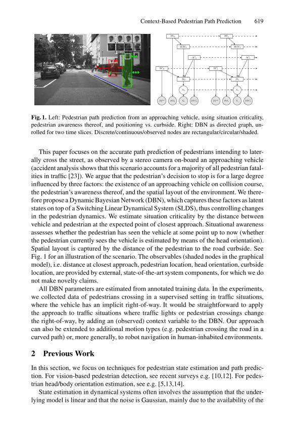
4.3 Evaluation

The dataset is divided into five sub-scenarios, listed in Table 1. Four sub-scenarios rep-resent “normal” pedestrian behaviors (e.g. the pedestrian stops if he is aware of a criticalsituation and crosses otherwise). The fifth sub-scenario is anomalous, since the pedes-trian crosses even though he is aware of the critical situation. We compare our proposedDBN with full context, referred to as SC+HSV+AC, to model variations with less con-text, and to a fixed velocity Kalman Filter with acceleration noise (see caption Table 1).

Leave-one-out cross-validation is used to separate training and test sequences, thoughsequences from the anomalous sub-scenario are excluded from the training data. Foreach time t with state Xt, we create a predictive distribution for Xt+tp at tp time stepsin the future by iteratively applying the Predict and Collapse steps (see Sec. 3.2), andonly Update with the DTC likelihood (Eq. (11)) using the predicted positions,

P tp|t(Xt+tp) ≡ P (Xt+tp |Y1:t). (20)

We define two performance metrics for a sequence, namely the Euclidean distance be-tween lateral predicted expected position xt+tp and lateral GT position Gt+tp , and thelog likelihood of G under the predictive distribution:

error(tp|t) = |E [P tp|t(xt+tp)

]−Gt+tp | (21)

predll(tp|t) = log[P tp|t(Gt+tp)

](22)

Note that the predictive log likelihood of [1] corresponds to predll(0|t).

Comparison of Model Variations. The results in Table 1 show the predictive log like-lihood predll for tp = 16 time steps (∼ 1 s) in the future, averaged over the second upto TTE = 0 when the pedestrian reaches the curb. In the first three normal sub-scenarios,


Table 1. Prediction log likelihood of the GT pedestrian position for tp = 16 frames (∼ 1 s) ahead,for different sub-scenarios (rows) and models (columns), for TTE ∈ [−15, 0]. The first four sub-scenarios contain “normal” pedestrian behavior. The fifth case is anomalous (lower likelihood isbetter). Model variations (best SLDS variant marked in bold): full context (SC+HSV+AC), nocurb (SC+HSV), only head (HSV), only criticality (SC), no context (SLDS), KF (LDS).

Sub-scenario SC+HSV+AC SC+HSV HSV SC SLDS LDSnon-critical, vehicle not seen, crossing -0.61 -0.53 -0.52 -0.59 -0.59 -1.90non-critical, vehicle seen, crossing -0.53 -0.45 -0.46 -0.47 -0.49 -1.93

critical, vehicle not seen, crossing -0.48 -0.34 -0.17 -0.59 -0.33 -1.88critical, vehicle seen, stopping -0.33 -0.70 -1.13 -0.80 -1.26 -1.88critical, vehicle seen, crossing -0.90 -0.27 -0.15 -0.25 -0.13 -1.88

all five SLDS-based models perform similarly, clearly outperforming the LDS (whichhas similar low likelihoods across the board, i.e. it is unspecific for any sub-scenario).However, in the fourth sub-scenario (pedestrian sees the vehicle in a critical situationand stops), the simpler DBNs have low predictive likelihoods, except for our proposedmodel. Without the full context, the other models are not capable to predict if, whereand when the pedestrian will stop. For the anomalous fifth sub-scenario, only the pro-posed model results in lower likelihood than for normal behavior, which is a usefulproperty for anomaly detection. A future driver warning strategy could benefit from themore accurate path prediction of our SC+HSV+AC model in high likelihood situations,whereas falling back to simpler models/strategies when anomalies are detected.

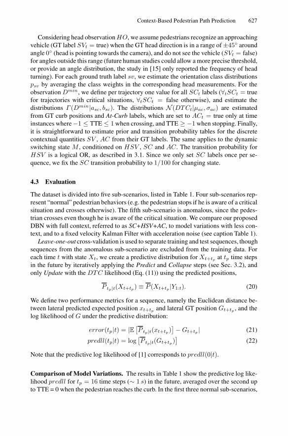
Fig. 2 illustrates a sequence from the stopping sub-scenario (fourth row in Table 1),with a snapshot just before (TTE = −20) and after (TTE = −9) the pedestrian be-comes aware of the critical situation. At TTE = −20, the predicted distributions ofall models are close together and indicate that the pedestrian continues walking (theLDS does so with high uncertainty). At TTE = −9, the mean position predictions ofthe LDS are furthest away from the GT (still within one std.dev. because of high un-certainty). The SLDS-only prediction shows a comparatively low uncertainty, but thepredicted means have a high distance to the GT (not within one std.dev.). Predictionsof the SC+HSV model are closer to the true positions, since it captures the situationalawareness of the pedestrian and therefore assigns a higher probability, compared toSLDS, to switch to the standing model ms. The SC+HSV+AC model makes the bestpredictions as it also anticipates where the pedestrian will stop, namely at the curbside.

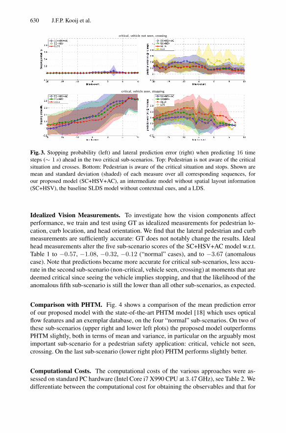
In the context of action classification, Fig. 3 shows for various model variations,(left) the standing probability Pt(Mt = ms), and (right) the error(tp|t) for predictionsmade tp = 16 frames ahead, plotted against the TTE. In the first sub-scenario (top row),the pedestrian crosses in a critical situation without seeing the approaching vehicle. Allmodels have a very low stopping probability, but since a few sequences have ambiguoushead observations, our proposed model does not exclude the possibility that the vehiclehas been seen. This translates to a higher stopping probability near the curb, and to ahigher error of the average prediction for a short while. Still, the model recuperates asthe pedestrian approaches the curb and shows no sign of slowing down, which informsthe model that the pedestrian did not see the vehicle (i.e. joint inference also means thatobserved motion dynamics can disambiguate low-level head orientation estimation). In


Fig. 2. Example of a pedestrian that will stop at the curb after becoming aware of a criticalsituation. Predictions are made tp = 16 (∼ 1 s) time steps ahead from different times t. Top left:Pedestrian with head detection bounding box (white), tracking bounding box (green), collapsedpredicted distribution of the SC+HSV+AC model (blue ellipses show one and two std.dev.) andcurb detection (blue line) made at time t = 12 (TTE = −20). Top center: The pedestrianbecame aware of the critical situation, shown is time step t = 23 (TTE = −9). Bottom left:Predictions (mean and std.dev.(shaded)) made at t = 12 (dashed green line and diamond) forthe lateral position at time t + tp (red diamond indicates the GT at t + tp) . Vertical black linedenotes the event. Black dots indicate position measurements, the black line the GT positions.Colored lines are predicted positions by different models. Bottom center: Predictions of the lateralposition at t + tp made from t = 23. Right: Inferred marginal distributions for the latent binaryvariables in the SC+HSV+AC model, using gray scale coded probability from 0 (black) to 1(white). Horizontal axis is time. Variable labels are True and False, and walking and standing.

the second sub-scenario (bottom row), the pedestrian is aware of the critical situationand stops at the curb. Now, all models show an increasing stopping probability towardsthe event point. In a few scenarios, the SLDS switches too early to the standing state,reacting to perceived de-acceleration (noise) of the pedestrian walking, hence the highstd. dev. of the SLDS over all sequences early on. However, on average the SLDS as-signs a higher probability to standing (> 0.5) than walking after the pedestrian hasalready reached the curb (TTE > 0). It can only react to changing dynamics, but notanticipate it. Our proposed model, on the other hand, gives the best action classification(highest stopping probability at TTE = 0). It anticipates the change in motion dynam-ics a few frames earlier as the SLDS, benefiting from the combined knowledge aboutsituation criticality and spatial layout. Further, the knowledge about the spatial layouthelps to keep the standing probability low while the pedestrian is still far away from thecurb. The model with limited context information ends up in between proposed modeland SLDS. Accordingly, our proposed model has the lowest prediction error (bottomright plot). Averaged over the sequences, it outperforms the baseline SLDS model byup to 0.39m (at TTE = 1) and the SC+HSV model with up to 0.16m (at TTE = −10).


critical, vehicle not seen, crossing

critical, vehicle seen, stopping

Fig. 3. Stopping probability (left) and lateral prediction error (right) when predicting 16 timesteps (∼ 1 s) ahead in the two critical sub-scenarios. Top: Pedestrian is not aware of the criticalsituation and crosses. Bottom: Pedestrian is aware of the critical situation and stops. Shown aremean and standard deviation (shaded) of each measure over all corresponding sequences, forour proposed model (SC+HSV+AC), an intermediate model without spatial layout information(SC+HSV), the baseline SLDS model without contextual cues, and a LDS.

Idealized Vision Measurements. To investigate how the vision components affectperformance, we train and test using GT as idealized measurements for pedestrian lo-cation, curb location, and head orientation. We find that the lateral pedestrian and curbmeasurements are sufficiently accurate: GT does not notably change the results. Idealhead measurements alter the five sub-scenario scores of the SC+HSV+AC model w.r.t.Table 1 to −0.57, −1.08, −0.32, −0.12 (“normal” cases), and to −3.67 (anomalouscase). Note that predictions became more accurate for critical sub-scenarios, less accu-rate in the second sub-scenario (non-critical, vehicle seen, crossing) at moments that aredeemed critical since seeing the vehicle implies stopping, and that the likelihood of theanomalous fifth sub-scenario is still the lower than all other sub-scenarios, as expected.

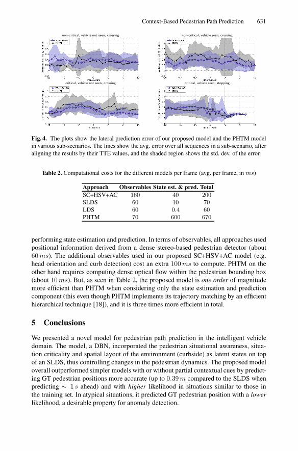
Comparison with PHTM. Fig. 4 shows a comparison of the mean prediction errorof our proposed model with the state-of-the-art PHTM model [18] which uses opticalflow features and an exemplar database, on the four “normal” sub-scenarios. On two ofthese sub-scenarios (upper right and lower left plots) the proposed model outperformsPHTM slightly, both in terms of mean and variance, in particular on the arguably mostimportant sub-scenario for a pedestrian safety application: critical, vehicle not seen,crossing. On the last sub-scenario (lower right plot) PHTM performs slightly better.

Computational Costs. The computational costs of the various approaches were as-sessed on standard PC hardware (Intel Core i7 X990 CPU at 3.47GHz), see Table 2. Wedifferentiate between the computational cost for obtaining the observables and that for


non-critical, vehicle not seen, crossing non-critical, vehicle seen, crossing

critical, vehicle not seen, crossing critical, vehicle seen, stopping

Fig. 4. The plots show the lateral prediction error of our proposed model and the PHTM modelin various sub-scenarios. The lines show the avg. error over all sequences in a sub-scenario, afteraligning the results by their TTE values, and the shaded region shows the std. dev. of the error.

Table 2. Computational costs for the different models per frame (avg. per frame, in ms)

Approach Observables State est. & pred. TotalSC+HSV+AC 160 40 200SLDS 60 10 70LDS 60 0.4 60PHTM 70 600 670

performing state estimation and prediction. In terms of observables, all approaches usedpositional information derived from a dense stereo-based pedestrian detector (about60ms). The additional observables used in our proposed SC+HSV+AC model (e.g.head orientation and curb detection) cost an extra 100ms to compute. PHTM on theother hand requires computing dense optical flow within the pedestrian bounding box(about 10ms). But, as seen in Table 2, the proposed model is one order of magnitudemore efficient than PHTM when considering only the state estimation and predictioncomponent (this even though PHTM implements its trajectory matching by an efficienthierarchical technique [18]), and it is three times more efficient in total.

5 Conclusions

We presented a novel model for pedestrian path prediction in the intelligent vehicledomain. The model, a DBN, incorporated the pedestrian situational awareness, situa-tion criticality and spatial layout of the environment (curbside) as latent states on topof an SLDS, thus controlling changes in the pedestrian dynamics. The proposed modeloverall outperformed simpler models with or without partial contextual cues by predict-ing GT pedestrian positions more accurate (up to 0.39m compared to the SLDS whenpredicting ∼ 1 s ahead) and with higher likelihood in situations similar to those inthe training set. In atypical situations, it predicted GT pedestrian position with a lowerlikelihood, a desirable property for anomaly detection.


We show that the proposed approach even slightly outperformed a state-of-the-artPHTM approach at less than a third of computational cost. These two approaches donot stand directly in competition, however, as they use different sources of informa-tion that could conceivably be combined. Further work involves the incorporation ofadditional scene context (e.g. traffic light, pedestrian crossing) and the extension of thebasic motion types of the SLDS (e.g. turning). We are encouraged that the presentedcontext-based models can play an important role in future generation driver warningand vehicle control strategies that save pedestrian lives.

References

1. Abbeel, P., Coates, A., Montemerlo, M., Ng, A.Y., Thrun, S.: Discriminative training ofKalman filters. In: Robotics: Science and Systems, pp. 289–296 (2005)

2. Antonini, G., Martinez, S.V., Bierlaire, M., Thiran, J.P.: Behavioral priors for detection andtracking of pedestrians in video sequences. IJCV 69(2), 159–180 (2006)

3. Ba, S., Odobez, J.: Multiperson visual focus of attention from head pose and meeting con-textual cues. IEEE PAMI 33(1), 101–116 (2011)

4. Bandyopadhyay, T., Won, K., Frazzoli, E., Hsu, D., Lee, W., Rus, D.: Intention-aware motionplanning. In: Algorithmic Foundations of Robotics X, pp. 475–491. Springer (2013)

5. Benfold, B., Reid, I.: Guiding visual surveillance by tracking human attention. In: Proc.BMVC (2009)

6. Bishop, C.M.: Pattern Recognition and Machine Learning, vol. 1. Springer (2006)7. Blackman, S., Popoli, R.: Design and Analysis of Modern Tracking Systems. Artech House

Norwood (1999)8. Boyen, X., Koller, D.: Tractable inference for complex stochastic processes. In: Proc. of UAI,

pp. 33–42. Morgan Kaufmann Publishers Inc. (1998)9. Dalal, N., Triggs, B.: Histograms of oriented gradients for human detection. In: Proc. CVPR,

pp. 886–893. IEEE (2005)10. Dollar, P., Wojek, C., Schiele, B., Perona, P.: Pedestrian detection: An evaluation of the state

of the art. IEEE PAMI 34(4), 743–761 (2012)11. Duda, R.O., Hart, P.E.: Use of the Hough transformation to detect lines and curves in pictures.

Commun. ACM 15(1), 11–15 (1972)12. Enzweiler, M., Gavrila, D.M.: Monocular pedestrian detection: Survey and experiments.

IEEE PAMI 31(12), 2179–2195 (2009)13. Enzweiler, M., Gavrila, D.M.: Integrated pedestrian classification and orientation estimation.

In: Proc. CVPR, pp. 982–989. IEEE (2010)14. Flohr, F., Dumitru-Guzu, M., Kooij, J.F.P., Gavrila, D.M.: Joint probabilistic pedestrian head

and body orientation estimation. In: IEEE Intell. Veh. (2014)15. Hamaoka, H., Hagiwara, T., Tada, M., Munehiro, K.: A study on the behavior of pedestrians

when confirming approach of right/left-turning vehicle while crossing a crosswalk. In: IEEEIntell. Veh., pp. 106–110 (2013)

16. Helbing, D., Molnar, P.: Social force model for pedestrian dynamics. Phys. Rev. E 51(5),4282 (1995)

17. Hirschmuller, H.: Stereo processing by semiglobal matching and mutual information. IEEEPAMI 30(2), 328–341 (2008)

18. Keller, C.G., Gavrila, D.M.: Will the pedestrian cross? A study on pedestrian path prediction.IEEE Trans. ITS 15(2), 494–506 (2014)


19. Kitani, K.M., Ziebart, B.D., Bagnell, J.A., Hebert, M.: Activity forecasting. In: Fitzgib-bon, A., Lazebnik, S., Perona, P., Sato, Y., Schmid, C. (eds.) ECCV 2012, Part IV. LNCS,vol. 7575, pp. 201–214. Springer, Heidelberg (2012)

20. Kohler, S., Schreiner, B., Ronalter, S., Doll, K., Brunsmann, U., Zindler, K.: Autonomousevasive maneuvers triggered by infrastructure-based detection of pedestrian intentions. In:IEEE Intell. Veh., pp. 519–526 (2013)

21. Kooij, J.F.P., Englebienne, G., Gavrila, D.M.: A non-parametric hierarchical model to dis-cover behavior dynamics from tracks. In: Fitzgibbon, A., Lazebnik, S., Perona, P., Sato, Y.,Schmid, C. (eds.) ECCV 2012, Part VI. LNCS, vol. 7577, pp. 270–283. Springer, Heidelberg(2012)

22. Lauritzen, S.L.: Propagation of probabilities, means, and variances in mixed graphical asso-ciation models. Journal of the American Statistical Association 87(420), 1098–1108 (1992)

23. Meinecke, M.M., Obojski, M., Gavrila, D.M., Marc, E., Morris, R., Tons, M., Lettelier, L.:Strategies in terms of vulnerable road user protection. In: EU Project SAVE-U, DeliverableD6 (2003)

24. Meuter, M., Iurgel, U., Park, S.B., Kummert, A.: Unscented Kalman filter for pedestriantracking from a moving host. In: IEEE Intell. Veh., pp. 37–42 (2008)

25. Minka, T.P.: Expectation propagation for approximate Bayesian inference. In: Proc. of UAI,pp. 362–369. Morgan Kaufmann Publishers Inc. (2001)

26. Oh, S.M., Rehg, J.M., Balch, T., Dellaert, F.: Learning and inferring motion patterns usingparametric segmental switching linear dynamic systems. IJCV 77(1-3), 103–124 (2008)

27. Pavlovic, V., Rehg, J.M., MacCormick, J.: Learning switching linear models of human mo-tion. In: Advances in NIPS, pp. 981–987 (2000)

28. Pellegrini, S., Ess, A., Schindler, K., Van Gool, L.: You’ll never walk alone: Modeling socialbehavior for multi-target tracking. In: Proc. ICCV, pp. 261–268 (2009)

29. Rosti, A.V.I., Gales, M.J.F.: Rao-Blackwellised Gibbs sampling for switching linear dynam-ical systems. In: Proc. of the IEEE ICASSP, vol. 1, pp. 809–812 (2004)

30. Schneider, N., Gavrila, D.M.: Pedestrian path prediction with recursive Bayesian filters:A comparative study. In: Weickert, J., Hein, M., Schiele, B. (eds.) GCPR 2013. LNCS,vol. 8142, pp. 174–183. Springer, Heidelberg (2013)

31. Schreiber, M., Knoppel, C., Franke, U.: LaneLoc: Lane marking based localization usinghighly accurate maps. In: IEEE Intell. Veh., pp. 449–454 (2013)

32. Tamura, Y., Le, P.D., Hitomi, K., Chandrasiri, N., Bando, T., Yamashita, A., Asama, H.:Development of pedestrian behavior model taking account of intention. In: IEEE IROS, pp.382–387 (2012)

33. Wohler, C., Anlauf, J.K.: A time delay neural network algorithm for estimating image-patternshape and motion. IVC 17(3-4), 281–294 (1999)

Documents

Context-Based Pedestrian Path Prediction - Gavrila · Context-Based Pedestrian Path Prediction Julian Francisco Pieter Kooij 1,2, ... goes beyond the state-of-the-art on pedestrian