ContentServer.asp 2

Journal of Applied Statistics, 2014Vol. 41, No. 1, 2–25, http://dx.doi.org/10.1080/02664763.2013.827160

Modelling oil and gas supply disruption risksusing extreme-value theory and copula

Nalan Gülpınara∗ and Kabir Katatab

aWarwick Business School, Coventry CV4 7AL, UK; bNigeria Deposit Insurance Corporation,Abuja, Nigeria

(Received 26 March 2013; accepted 17 July 2013)

In this paper, we are concerned with modelling oil and gas supply disruption risks using extreme-valuetheory and copula. We analyse financial and volumetric losses due to both oil and gas supply disruptionsand investigate their dependence structure using real data. In order to illustrate the impact of crude oiland natural gas supply disruptions on an energy-dependent economy, Nigeria is considered as a casestudy. Computational studies illustrate that the generalized extreme-value distribution anticipates higherfinancial losses and extreme-value copulas produce the best fit for financial and volumetric losses comparedwith normal copulas. Moreover, multivariate financial losses exhibit stronger positive dependence thanvolumetric losses.

Keywords: risk management; supply disruptions; copula; extreme-value theory

1. Introduction

In general terms, disruption is defined as breakdown of production operations within a supplychain. Supply disruptions are extreme events that are associated with the flow and transformationof different goods or raw materials. Extreme events are rare, severe and outside normal experiencethat involves high degree of uncertainty caused by limited information [4]. Supply disruption riskis considered as an extreme case of operational risk. According to Kleindorfer and Saad [26],disruption risk arises due to equipment malfunctions or discontinuities in supply and human-centred issues such as strikes and fraud. They also mentioned that natural hazards, terrorism andpolitical instability may cause disruption risk.

Supply disruptions in petroleum markets have been financially catastrophic and had a significantfinancial impact on energy-dependent economies. Several oil-dependent companies have facedrevenue and cash-flow crises because of oil and gas disruptions.As reported in Energy InformationAdministration (EIA) [12], Nigeria lost an estimated 16 billion dollars in export revenues due toshut-in oil production from December 2005 toApril 2007. During that period, several oil producing

∗Corresponding author. Email: [email protected]

© 2013 Taylor & Francis

Journal of Applied Statistics 3

companies suffered the majority of shut-in oil production; for instance, Shell lost 477,000 barrelsper day (bbl/d) followed by Chevron 70,000 bbl/d andAgip 40,000 bbl/d. It is well known that thedecline in production and supply of crude oil (CO) and natural gas (NG) in any major oil producingcountry has had an impact on the world oil prices and other sectors of the world economy. Forinstance, Brent Blend price increased from 58.69/bbl (30 December 2005) to 65.08/bbl (30January 2006) due to actual and potential disruptions to CO supplies from Nigeria, the North Seaand Australia [11]. According to Geman [18], among other reasons, price of CO increased bymore than 500% in less than four years due to supply disruptions in Nigeria.

Most energy companies engage in oil and gas exploration and trading.A catastrophic CO supplydisruption by itself may drive an exploration firm to bankruptancy or an oil and gas producingcountry to lose a large revenue. Although natural gas is not always physically found togetherwith CO, the two products nevertheless form a financial portfolio for most energy-dependentcompanies. Historically, catastrophic disruptions in CO and NG tend to occur together, signifyingdependence. For instance, hurricanes Katrina and Rita shut down oil and gas production fromthe Outer Continental Shelf in the Gulf of Mexico and consequently, 25% of US CO productionand 20% of NG were simultaneously affected [28]. A disruption in the production of CO mighttherefore have the same effect in the production of NG and vice versa.

Energy-dependent economies and energy security strategies need to cope with supply risksof simultaneous oil and gas shortages. Quantitative modelling of supply disruption risks andassociated losses is essential for governments and energy market participants. It is of paramountimportance to both oil and gas consumers and producers including financial institutions and marketmakers to accurately model supply disruption risks. A major uncertainty in national budgeting,insurance of national or company revenues and building stockpiles can be eliminated throughaccurate estimation of supply disruption risks. In addition, insurance companies, traders and bankscan accurately forecast their earnings and cash-flow related to oil and gas portfolios. During theStanford Energy Modelling Forum in 2005, energy market and geopolitical experts recognized theimportance of using quantitative techniques and developed risk assessment framework utilizingexpert judgement to characterize the likelihood, magnitude and duration of potential oil supplydisruptions [3]. It was also noted at the forum that, despite the huge losses as well as the needfor security and policy implications, there was no reliable quantitative modelling of oil supplydisruptions prior to 2005. There had been only three formal probability assessments consideredfor oil disruptions in the US-DOE/Interagency study in 1990.

Probability theory, fault tree, event tree assessments and decision tree analysis have been devel-oped to measure disruption risk [26]. The reader is referred to Grossi and Kunreuther [25] fordetailed discussion on modelling catastrophic events. Several researchers have investigated theimpact of supply disruptions in petroleum markets. Reister [39] develops a general equilibriummodel for oil price jumps caused by supply disruptions. Curlee et al. [8] apply a linear program-ming model to address oil supply disruptions. Greene et al. [23] consider Monte Carlo simulationfor risk analysis of world conventional oil resource production from 2000 to 2050. However, noneof these efforts have quantitatively measured CO or NG supply risks.

In this paper, we are concerned with quantitative modelling of oil and gas supply disruption risksusing extreme-value theory (EVT) and copula. The EVT models are used to describe univariate COand NG supply disruption risks in terms of volumetric and financial losses. The copula functionsmodel the multivariate dependence between CO and NG supply disruption risks. In order to gainfurther insights into how supply disruption risks can affect an oil and gas dependant economy,Nigeria is considered as a case study.

The rest of the paper is organized as follows. A brief introduction to the notion of EVT andcopula functions is provided in Section 2. Section 3 presents empirical analysis of oil and gassupply disruptions in case of Nigeria using EVT and copula functions. Section 4 concludes thepaper with a short summary of the findings.

4 N. Gülpınar and K. Katata

2. A brief primer on EVT and copula

A brief introduction to the main ideas of EVT and copula functions is provided next.

2.1 Extreme-value theory

EVT is an established field of statistics based on rigorous mathematical methods [32], and hasbeen widely used in engineering, finance and insurance sectors to analyse rare and extremecatastrophic events; see for instance, El-Gamal et al. [13], Engeland et al. [17], Clemente andRomano [6], Mohtadi and Murshid [35] and Meela et al. [34]. It has also been considered tomeasure market and price risks in financial markets. Gencay and Selcuk [19] investigate therelative performance of nine different emerging markets using EVT and value-at-risk (VaR).Ren and Giles [40] introduce extreme-value analysis for estimating daily Canadian CO prices.Marimoutoua et al. [29] model VaR for long and short trading positions in oil market by applyingboth unconditional and conditional EVT models.

EVT is used to describe extreme events unlike normal or log-normal distribution that oftenunder-estimates risk of extreme events [14]. Most importantly, EVT provides a good fit for thetails of distributions and makes the best use of data about the extreme phenomena [16]. Onthe other hand, it involves some limitations. For instance, EVT like other statistical approachespossesses model uncertainty due to either wrong calibration or data scarcity. The reader is referredto Embrechts [14] for more details on its potential and limitations.

There are two main approaches for modelling extreme events, namely block maxima andpeak over threshold. The block maxima approach is used for modelling the largest observationscollected from samples that are identically distributed and modelled by generalized extreme-value(GEV) distribution. The peak over threshold considers all large observations that exceed specifiedthreshold and is modelled by generalized Pareto distribution (GPD). Several researchers such asMcNeil and Saladdin [33] and Coles [7] have contributed abundant theoretical discussion on EVTmodels. In this section, we briefly summarise these models and relevant risk measures.

2.1.1 GEV distribution

GEV is the limiting distribution of normalized extrema. The GEV distribution is used to model thesmallest or largest value among a large set of independent, identically distributed random valuesrepresenting measurements or observations. This distribution is described by location, scale andshape parameters.

Let x be a sequence of identical and independent random variables of x1, x2, . . . , xn with acommon distribution function F(x), which denotes an unknown distribution of x. Let μ representthe location parameter of random variable x. The tail index (also called shape) parameter of thedistribution is denoted by ξ . The sample maxima of x is Mn = max(x1, x2, . . . , xn).

Assume that x satisfies the condition 1 + ξ(x − μ)/σ > 0 where σ is the scale parameter. LetH be a non-degenerate distribution function that is defined as

Hξ ,μ,σ (x) =

⎧⎪⎪⎪⎨⎪⎪⎪⎩

exp

(−

(1 + ξ

x − μ

σ

)−1/ξ)

if ξ �= 0,

exp

(− exp

(−x − μ

σ

))if ξ = 0.

(1)

For independent and identically distributed random variables (x1, x2, . . . , xn), if there exists con-

stants an > 0 and bn ∈ R such that a−1n (Mn − bn)

d−→ H.According to Fisher–Tippet theorem [32],as n increases, the type of GEV distribution of extremes (Mn) under general conditions is


determined by the value of shape parameter. If ξ > 0, then H is named as the Frechet distributionthat has heavy tails such as Levy, Pareto and t-distributions. When ξ = 0, Gumbel distribution isobtained. The GEV distribution in this case has thin-tails that are usually obtained in normal andlog-normal distributions. If ξ < 0, then the distribution is called Weibull that has lighter tails thanthe Gumbel distribution.

2.1.2 Generalized Pareto distribution

GPD describes the behaviour of large observations which exceed high thresholds. Provided thethreshold is high enough, the GPD is regarded as the natural distribution for modelling excesslosses.

Consider X and � to be a random variable and threshold, respectively. Define X − � to be theexcess loss over the threshold, known as the exceedance denoted by x. Assume that x is strictlypositive. Let F(x) be the distribution function of X . The distribution function of excess losses overthe threshold � is defined as

F�(x) = Pr{X − � ≤ x | X > �} = F(x + �) − F(�)

1 − F(�). (2)

According to the Gnedenko–Picklands–Balkema–de Hann theorem, as � gets large, the distri-bution F�(x) converges to a GPD. This distribution involves two parameters: a positive scaleparameter and tail index. Let ξ and β be the shape and scale parameters of the GPD, respectively.Assume that the following conditions hold:

x − � ≥ 0 if ξ ≥ 0, and

0 ≤ x − � ≤ −β

ξif ξ < 0. (3)

Then the GPD can be defined as follows:

Gξ ,β(x) =

⎧⎪⎪⎪⎨⎪⎪⎪⎩

1 −(

1 + ξx

β

)−1/ξ

if ξ �= 0,

1 − exp

(− x

β

)if ξ = 0.

(4)

The GPD subsumes different distributions as special cases depending on the scale parameter ξ .If ξ > 0 (or ξ < 0), then the GPD is equivalent to ordinary Pareto distribution (or Pareto type IIdistribution). If ξ = 0, it becomes the exponential distribution.

2.1.3 Risk measures

The quantiles of distribution functions are the most frequently used metrics for estimating financialrisk. In this section, we describe the risk measures associated with losses for both generalizedPareto and GEV distributions. For extensive discussion and derivation of the quantiles, the readeris referred to McNeil et al. [32].

2.1.3.1 GEV risk measures Return level and VaR are the risk measures associated with a GEVdistribution. Return level represents the maximum loss of a series or a portfolio. Let n be the blocklength of maxima that follows a GEV distribution. The distribution function Hξ ,μ,σ is defined as


in Equation (1). The return level, denoted by Rn,k , identifies the position expected to be exceededin one out of k periods of whole length n. Moreover, Rn,k is a quantile of this distribution and isdefined by a simple function of its parameters as follows:

Rn,k =

⎧⎪⎪⎪⎨⎪⎪⎪⎩

μ −(

σ

ξ

) [1 −

(− log

(1

k

))]−ξ

if ξ �= 0,

μ − σ log

[− log

(1 − 1

k

)]if ξ = 0.

(5)

There are two approaches used for stress-testing the financial losses: the return-level estimationand return-period problems. In the first approach, we estimate the magnitude of stress event basedon a pre-defined frequency of its occurrence. In the return-period problem, the size of the stressevent is defined and the frequency of occurrence is estimated. For instance, a 10-year return levelis a level, which at average, should only be exceeded in one year every 10 years. This level may ormay not be exceeded more than once in a year, depending on data dependencies and clustering.

VaR is extensively used in financial applications to portray the risk of an asset or portfolio asa single figure. VaR defines the lowest quantile of the potential losses that can occur during aspecified time period at a given confidence level. Let x be a random variable with continuousdistribution function F. For a specific confidence level p, VaRp represents the pth quantile of thedistribution F and is formulated as

VaRp = F−1(1 − p), (6)

where the inverse of the distribution function F−1 is called a quantile function. For any (cumulative)probability p, we can obtain the quantiles associated with the GEV distribution by setting the left-hand side of Equation (1) to p and then solving it for x. The values of x represent the quantilesbased on pre-determined p. Therefore, the VaR for GEV distribution, VaRGEV

p , is found as

VaRGEVp =

⎧⎪⎨⎪⎩

μ −(

σ

ξ

)[1 − (− log(p))−ξ ] if ξ �= 0,

μ − σ log[− log(p)] if ξ = 0.(7)

2.1.3.2 GPD risk measures VaR and conditional value-at-risk (CVaR) are the two risk mea-sures that can be computed using the GPD. Let N� be the number of observations in excess ofthreshold value �. The confidence level is selected as p. Let β denote a positive scale parameter.VaR associated with the GPD, denoted by VaRGPD

p , is computed as follows:

VaRGPDp = � + β

ξ

[(n

N�

(1 − p)

)−ξ

− 1

]. (8)

CVaR (also called expected shortfall) estimates the potential size of the loss exceeding VaR thatdefines unconditional VaR. In this case, expected shortfall is equal to VaR plus the mean excessloss over VaR. Assuming that ξ ≤ 1, the expected shortfall denoted by ESGPD

p is formulated as

ESGPDp = VaRGPD

p

1 − ξ+ β − ξ�

1 − ξ. (9)

VaR violates the subadditive property of risk measures; that is risk of sum of random variables isalways less than or equal to the sum of the risk of individual random variables. Expected shortfallinstead of VaR is used as a coherent risk measure [2].


Parameters of the EVT distributions can be estimated by various methods such as maximumlikelihood and probability weighted moments. The reader is referred to McNeil et al. [32] fordetailed discussion on implementing these methods.

2.2 Copula functions

Quantitative models are based on univariate or multivariate distributional assumption of the under-lying random variables. In practice, particularly for financial applications, it is common to assumethat the variables are independent or the dependence between random variables is described bynormal distribution [10]. On the other hand, univariate financial data usually have heavier tailsthat cannot be described by normal distribution whereas in multivariate cases, variables are depen-dent [16]. For instance, Alexander [1] shows that the dependence between prices of futures onCO and NG is strong and cannot be modelled correctly by a bivariate normal distribution. Aswidely recognized in finance and insurance, incorrect distributional assumptions and/or specifi-cation of dependence relationship may result in gross underestimation or mispricing of financialinstruments.

Copula therefore overcomes the restrictions of multivariate dependence analysis by specifyingdependence structures that are dictated by the data characteristics. Beyond linear correlationand stress-testing [20], copula is also used for pricing of products on multiline/multivariatedistribution [5,24] and for risk management [16,27].

Copula is simply the distribution function of random variables with uniform marginals. Giventwo or more marginal distributions (e.g. EVT) that model individual movement of randomvariables, a copula function describes how the distributions ‘relate together’ to determine themultivariate distribution. The ability of a copula to separate the dependence structure from themarginal behaviour in a multivariate distribution is due to Sklar’s theorem presented below.

Let X and Y be random variables with continuous marginals Fx = u and Fy = v. Accordingto Sklar’s theorem, their joint distribution function F(x, y) can be written in terms of a uniquefunction C(u, v) as

F(x, y) = C(u, v).

The function C(u, v) is called the copula of F(x, y) and describes how F(x, y) is coupled with themarginal distribution functions Fx(x) and Fy(y). According to this theorem, the selection of thedependence structure and the choice of the univariate distributions can be independent of eachother. For instance, C(u, v) might be from Gumbel family of copulas, whereas Fx(x) might benormally distributed and Fy(y) is a Gamma distributed variable. Selection of an appropriate modelthat characterizes the dependence between X and Y can be independent of the choice of marginaldistributions.

There are several classes of copula functions. In this paper, we consider Archimedean copulasin the bivariate case (Clayton and Gumbel), meta-elliptical (normal) and extreme-value copulas(Gumbel, Galambos and Husler–Reiss). Although Gumbel and normal copulas are widely usedin finance, extreme-value copulas extend the univariate EVT technique [27].

Extreme-value copulas are the limits of copulas of component wise maxima in independentrandom samples, and provide appropriate models for the dependence structure between rareextreme events.

The Archimedean copula family has a simple closed form and can be stated directly. For−1 ≤ θ < ∞, the Clayton copula is defined as

C(u, v) = max[−(u−θ + v−θ − 1)−1/θ , 0].Note that Gumbel belongs to a family of both Archimedian and extreme-value copulas. BothClayton and Gumbel are asymmetric copulas, and exhibit greater tail dependence. In Gumbel, the


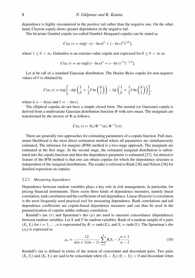
dependence is highly encountered in the positive tail rather than the negative one. On the otherhand, Clayton copula shows greater dependence in the negative tail.

The bivariate Gumbel copula (so-called Gumbel–Hougaard copula) can be stated as

C(u, v) = exp[−((− ln u)θ + (− ln v)θ )1/θ ],

where 1 ≤ θ < ∞. Galambos is an extreme-value copula and expressed for 0 ≤ θ < ∞ as

C(u, v) = uv exp[((− ln u)θ + (− ln v)−θ )−1/θ ].

Let φ be cdf of a standard Gaussian distribution. The Husler–Reiss copula for non-negativevalues of θ is obtained by

C(u, v) = exp

[−uφ

(1

θ+ 1

2θ ln

(u

v

))− vφ

(1

θ+ 1

2θ ln

(u

v

))],

where u = − ln(u) and v = − ln(v).The elliptical copulas do not have a simple closed form. The normal (or Gaussian) copula is

derived from a multivariate Gaussian distribution function � with zero mean. The marginals aretransformed by the inverse of � as follows:

C(u, v) = Nθ (�−1(u), �−1(v)).

There are generally two approaches for estimating parameters of a copula function. Full max-imum likelihood is the most direct estimation method where all parameters are simultaneouslyestimated. The inference for margins (IFM) method is a two-stage approach. The marginals areestimated at the first stage. At the second stage, the estimated marginal distribution is substi-tuted into the copula function and then the dependence parameter is estimated [27]. An attractivefeature of the IFM method is that one can obtain copulas for which the dependence structure isindependent of the marginal distributions. The reader is referred to Rank [38] and Nelsen [36] fordetailed exposition on copulas.

2.2.1 Measuring dependence

Dependence between random variables plays a key role in risk management, in particular, forpricing financial instruments. There exists three kinds of dependence measures, namely linearcorrelation, rank correlation and the coefficients of tail dependence. Linear (Pearson’s) correlationis the most frequently used practical tool for measuring dependence. Rank correlations and taildependence coefficients are copula-based dependence measures and can thus be used in theparametrization of copulas unlike ordinary correlation.

Kendall’s tau (τ ) and Spearman’s rho (ρ) are used to measure concordance (dependence)between random variables. Let X and Y be random variables. Rank of a random sample of n pairs(Xi, Yi) for i = 1, . . . , n is represented by Ri = rank(Xi), and Si = rank(Yi). The Spearman’s rho(ρn) is expressed as

ρn = 12

n(n + 1)(n − 1)

n∑i=1

RiSi − 3n + 1

n − 1. (10)

Kendall’s tau is defined in terms of the notion of concordant and discordant pairs. Two pairs(Xi, Yi) and (Xj, Yj) are said to be concordant when (Xi − Xj) (Yi − Yj) > 0 and discordant when


(Xi − Xj) (Yi − Yj) < 0. Let Pn and Qn be the number of concordant and discordant pairs,respectively. The Kendall’s tau (τn) is formulated as follows:

τn = Pn − Qn(n2

) = 4

n(n − 1)Pn − 1. (11)

The rank-based measures (Kendall’s tau and Spearman’s rho) provide the best alternatives tolinear correlation for measuring dependence of nonelliptical distributions. Linear correlation isonly ideal for elliptical distributions while most random variables are not elliptically distributed.Linear correlation is invariant under strictly linear transformation, but not under general or non-linear transformations. The variances of X and Y must be finite or the linear correlation is notdefined. For heavy-tailed distributions, linear correlation coefficient is not defined because ofinfinite second moments.

According to Schmidt [41], rank and nonlinear (Pearsons) correlations are the ideal tools formeasuring dependence between random variables. The rank correlations satisfy all the dependenceproperties mentioned above [16]. Moreover, they are invariant under monotonic transformationsand can handle perfect dependence reasonably well.

Tail dependence is frequently observed in financial and operational risk data. When extremeevents occur, the response from the market is usually asymmetric. Tail dependence measures theamount of dependence for extreme co-movements in the lower-left quadrant tail or upper-rightquadrant tail of a bivariate distribution. It is of importance because it is relevant for the studyof dependence between extreme values. Tail dependence expresses the probability of having ahigh (low) extreme value of a series given that a high (low) extreme value of another series hasoccurred. The higher probability of joint extreme observations as compared with the Gaussian(normal) copula is known as positive tail dependence. Normal and Frank copulas impose zerotail dependence whereas other copulas impose zero tail dependence in one tail. For instance,the Gumbel copula has upper left tail dependence, while the Clayton copula has lower right taildependence. Gaussian copula on the other hand exhibits no tail dependence [16].

3. Empirical analysis of oil and gas supply disruptions

3.1 Design of experiments and disruption data

We conduct a series of computational experiments to empirically analyse oil and gas supplydisruption risks. Specifically, we aim to answer the following questions:

• How can financial losses due to (univariate and multivariate) CO and NG supply disruptionsbe modelled? How much money does an oil producing company or country lose because ofsupply disruptions? At what probability?

• What is the quantity of CO and NG that an oil producing company or country may lose becauseof supply disruptions? At what probability?

• Is there a dependence between oil and gas supply disruption risks? How can the joint risk anddependence structure of the two extreme events be captured in terms of volumetric losses?

For empirical analysis of oil and gas supply disruption risks, we consider a case study of Nigeriathat is the 11th largest supplier of CO to the world, according to BP Statistical Review in 2007.Data for CO supply disruption are gathered from EIA in terms of losses due to all activities andevents that caused disruption in the production of CO in Nigeria from January 1996 to 2007.The NG disruption data as a percentage of gross production is collected from Nigeria NationalPetroleum Corporation (NNPC) Annual Statistical Bulletin that is available from the web site


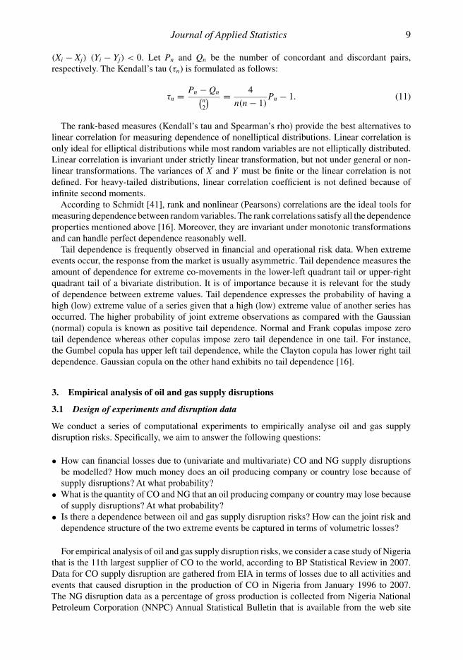
Figure 1. Time series of oil and gas supply disruption data.

http://www.nnpcgroup.com. It consists of observations as a result of flaring and venting of NG inNigeria from 1996 to 2007.

Figure 1 displays the financial losses due to CO supply disruptions (left) and the volumetriclosses in the supply of NG (right). The total NG and CO disruptive events during that period arecountered as 84 and 43, respectively. As can be seen from Figure 1, data for oil and gas supplydisruptions show the same characteristics as data for any operational risk [15]. Losses clearlyshow extremes and portray a tendency to increase over time. In addition, the loss occurrencetimes are also irregularly spaced in time.

The descriptive statistics of CO and NG disruption data in terms of financial and volumetriclosses are summarized in Table 1.

The summary statistics in Table 1 clearly show that normal or log-normal distribution does notfit the disruption data. In addition, the disruptions are independent and identically distributed (iid)satisfying a crucial requirement for the EVT analysis. This can be established on two grounds.First, the time lag between successive disruptions is at minimum a week that is sufficient enoughto ensure independence [17]. This means that disruptions that happen within a week are assumedto belong to the same event. Second, Ljung–Box–Pierce Q-test can be used to establish correlationstructure of the data. The experiments using Ljung–Box–Pierce Q-test reveal no significant cor-relation in the raw series when tested for up to 10, 15 and 20 lags of the autocorrelation functionat the 0.05 level of significance.

For the sake of completeness, it is worthwhile to mention that the Ljung–Box Q-test examinesthe dependence (correlation) structure of a time series. If a time series is serially uncorrelated, nolinear function of the lagged variables can account for the behaviour of the current variable. Fora serially independent time series, there is no relationship between the current and past variables.

Since our analysis is for longer horizons, a non-conditional approach is applied. This providesstable estimates through time requiring less frequent updates as suggested by Gilli and Kellezi [22]

Table 1. Descriptive statistics of CO and NG supply disruptions.

Financial loss Volumetric loss

NG (billion standardSummary statistics CO (US$ millions) NG (US$ millions) CO (1000s barrels) cubic feet)

Mean 109.69 320.52 164.50 98.99Standard deviation 229.90 376.24 167.14 87.29Skewness 4.77 1.24 1.52 0.66Kurtosis 27.61 3.76 4.85 3.25Median 31.92 189.65 106.00 48.70Minimum 3.03 90.45 9.00 1.86Maximum 1440.90 550.59 700.00 321.87

http://www.nnpcgroup.com


and Danielsson and de Vries [9]. It is worthwhile to note that a conditional approach (developedby McNeil and Frey [31]) could have been considered if the iid requirement was not satisfied.

As reported by McNeil and Saladin [33], for heavy-tailed distributions, the method of probabilityweighted moments gives biased parameter estimates while maximum likelihood is consistent.Therefore, we apply the maximum likelihood method to estimate model parameters for the GPDand the GEV distribution and to construct joint confidence intervals of the estimates.

3.2 Modelling univariate financial losses using EVT

This section is concerned with modelling univariate financial losses due to CO and NG supplydisruptions using EVT. We first undertake a series of tests using exploratory techniques thatprovide useful preliminary information about the disruption data, especially at the tail. Then thedisruption data are fit to the GPD and the GEV distribution and the forecasted losses obtained byvarious risk metrics are examined at various probabilities. Analysis of the empirical experimentsbased on the EVT distributions follows.

3.2.1 Exploratory data analysis

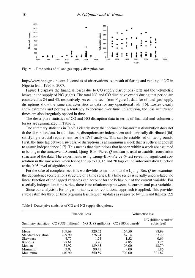
We consider a quantile–quantile (QQ-)plot to examine whether the sample comes from the expo-nential distribution (i.e. a distribution with a medium-sized tail). The QQ-plot of CO (top) andNG (bottom) disruption data against standard exponential quantiles presented in Figure 2 (left)has a concave departure. This implies that data follow a heavy-tailed distribution.

We carry on exploratory data analysis using a mean excess function to establish the heavinessand lightness of the distribution’s tails for choosing suitable threshold. The mean excess functionis defined as the ratio of the sum of the exceedances (over threshold) to the number of data pointswhich exceed the specified threshold. The sample mean excess function of CO (top) and NG(bottom) supply disruption data is plotted in Figure 2 (right). It can be easily seen that the samplemean excess function of disruption data has an upward slope. This implies that the disruption datafollows a GPD.

Figure 2. QQ-plots (left) and sample mean excess functions (right) of CO (top) and NG (bottom) disruptions.


Next, we fit CO and NG disruption data to the EVT distributions (generalized Pareto and GEV)and estimate the associated financial losses at various probabilities.

3.2.2 Generalized Pareto distribution

The parameters of GPD are obtained by fitting the exceedances over the threshold. A choice ofthreshold plays an important role on the degree of accuracy. If a low threshold is considered, theestimation becomes more precise but the number of observations (exceedances) increases. In addi-tion, a low threshold introduces some observations from the centre of the distribution and the esti-mation becomes biased. On the other hand, a high threshold implies fewer observations at the tail.

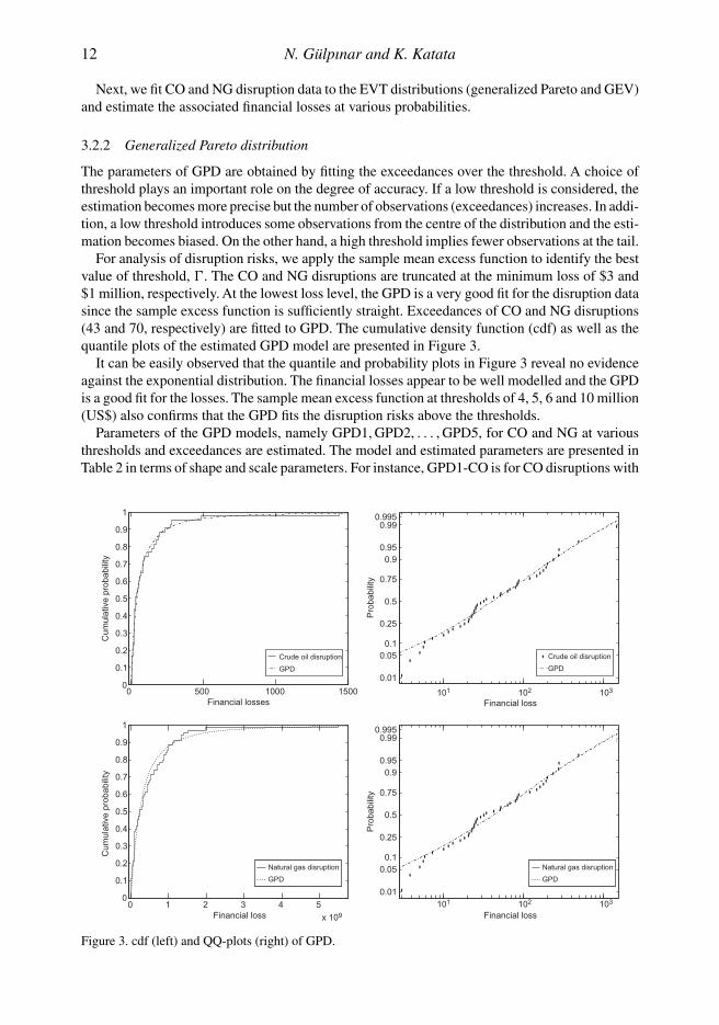
For analysis of disruption risks, we apply the sample mean excess function to identify the bestvalue of threshold, �. The CO and NG disruptions are truncated at the minimum loss of $3 and$1 million, respectively. At the lowest loss level, the GPD is a very good fit for the disruption datasince the sample excess function is sufficiently straight. Exceedances of CO and NG disruptions(43 and 70, respectively) are fitted to GPD. The cumulative density function (cdf) as well as thequantile plots of the estimated GPD model are presented in Figure 3.

It can be easily observed that the quantile and probability plots in Figure 3 reveal no evidenceagainst the exponential distribution. The financial losses appear to be well modelled and the GPDis a good fit for the losses. The sample mean excess function at thresholds of 4, 5, 6 and 10 million(US$) also confirms that the GPD fits the disruption risks above the thresholds.

Parameters of the GPD models, namely GPD1, GPD2, . . . , GPD5, for CO and NG at variousthresholds and exceedances are estimated. The model and estimated parameters are presented inTable 2 in terms of shape and scale parameters. For instance, GPD1-CO is for CO disruptions with

0 500 1000 15000

0.1

0.2

0.3

0.4

0.5

0.6

0.7

0.8

0.9

1

Financial losses

Cum

ulat

ive

prob

abili

ty

0

0.1

0.2

0.3

0.4

0.5

0.6

0.7

0.8

0.9

1

Cum

ulat

ive

prob

abili

ty

Crude oil disruption

GPD

101 102 103

0.01

0.050.1

0.25

0.5

0.75

0.90.95

0.990.995

Financial loss

101 102 103

Financial loss

Pro

babi

lity

Crude oil disruption

GPD

0 1 2 3 4 5

x 109Financial loss

Natural gas disruption

GPD

Natural gas disruption

GPD

0.01

0.050.1

0.25

0.5

0.75

0.90.95

0.990.995

Pro

babi

lity

Figure 3. cdf (left) and QQ-plots (right) of GPD.


Table 2. Model and estimated parameters for various GPD models.

Model parameters Estimated parameters

Models Threshold Excesses Shape SE CI Scale SE CI

GPD1-CO 3 43 0.71 0.28 (0.17, 1.25) 40.24 12.63 (22.57, 71.73)GPD2-CO 4 41 0.67 0.27 (0.14, 1.19) 44.65 13.16 (25.16, 79.23)GPD3-CO 5 41 0.71 0.28 (0.15, 1.27) 41.71 12.63 (23.04, 75.51)GPD4-CO 6 38 0.61 0.26 (0.10, 1.13) 51.16 15.00 (28.80, 90.88)GPD5-CO 10 37 0.72 0.30 (0.13, 1.31) 44.37 14.24 (23.65, 83.24)GPD1-NG 1 70 0.46 0.13 (0.04, 1.75) 27.96 7.12 (1.87, 46.33)GPD2-NG 2 69 0.43 0.11 (0.03, 1.84) 29.21 7.63 (2.38, 52.38)GPD3-NG 5 67 0.36 0.09 (0.01, 1.77) 33.14 6.21 (2.72, 61.15)GPD4-NG 6 66 0.36 0.08 (0.01, 1.71) 32.85 6.75 (2.90, 62.10)GPD5-NG 10 64 0.33 0.07 (0.02, 1.64) 35.02 6.61 (2.31, 76.08)

threshold of 3 and 43 exceedances. Abbreviations SE and CI represent the estimated ‘standarderrors’ and ‘confidence interval’, for each model, respectively.

As McNeil [30] and Coles [7] suggest the shape parameter represents the major component ofuncertainty in EVT. From Table 2, one can easily see that the shape parameter, standard errors(SEs) and confidence intervals (CIs) are consistent for all models. This consistency is obtained asa consequence of GPD having a good fit to the disruptions at various exceedances and thresholds.We also observe that GPD5-CO and GPD1-NG capture large losses and involve the highest shapeparameters and SEs as 0.72 and 0.30 for CO and 0.46 and 0.13 for NG, respectively. Moreover,supply disruption due to NG possesses much lower shape parameter than CO supply disruptionover all models. This implies heavier losses due to CO supply disruptions.

3.2.3 GEV distribution

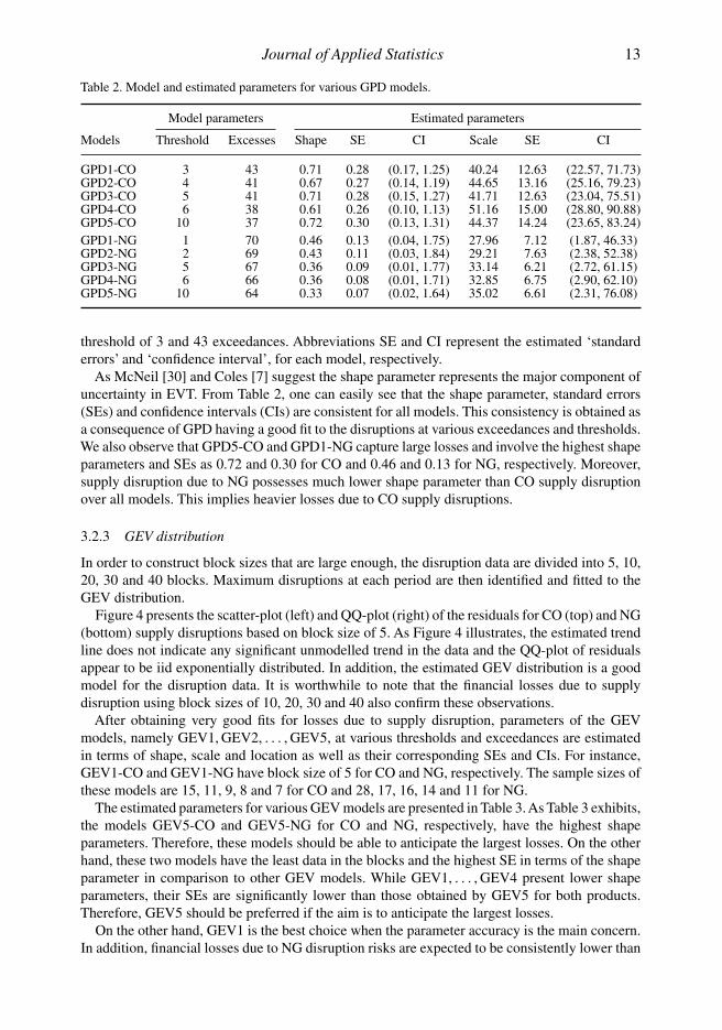
In order to construct block sizes that are large enough, the disruption data are divided into 5, 10,20, 30 and 40 blocks. Maximum disruptions at each period are then identified and fitted to theGEV distribution.

Figure 4 presents the scatter-plot (left) and QQ-plot (right) of the residuals for CO (top) and NG(bottom) supply disruptions based on block size of 5. As Figure 4 illustrates, the estimated trendline does not indicate any significant unmodelled trend in the data and the QQ-plot of residualsappear to be iid exponentially distributed. In addition, the estimated GEV distribution is a goodmodel for the disruption data. It is worthwhile to note that the financial losses due to supplydisruption using block sizes of 10, 20, 30 and 40 also confirm these observations.

After obtaining very good fits for losses due to supply disruption, parameters of the GEVmodels, namely GEV1, GEV2, . . . , GEV5, at various thresholds and exceedances are estimatedin terms of shape, scale and location as well as their corresponding SEs and CIs. For instance,GEV1-CO and GEV1-NG have block size of 5 for CO and NG, respectively. The sample sizes ofthese models are 15, 11, 9, 8 and 7 for CO and 28, 17, 16, 14 and 11 for NG.

The estimated parameters for various GEV models are presented in Table 3. As Table 3 exhibits,the models GEV5-CO and GEV5-NG for CO and NG, respectively, have the highest shapeparameters. Therefore, these models should be able to anticipate the largest losses. On the otherhand, these two models have the least data in the blocks and the highest SE in terms of the shapeparameter in comparison to other GEV models. While GEV1, . . . , GEV4 present lower shapeparameters, their SEs are significantly lower than those obtained by GEV5 for both products.Therefore, GEV5 should be preferred if the aim is to anticipate the largest losses.

On the other hand, GEV1 is the best choice when the parameter accuracy is the main concern.In addition, financial losses due to NG disruption risks are expected to be consistently lower than


0 5 10 15−0.5

0

0.5

1

1.5

2

2.5

3

3.5

4

Financial loss

Res

idua

ls

−0.5

0

0.5

1

1.5

2

2.5

3

3.5

4

Res

idua

ls

0 0.5 1 1.5 2 2.5 3 3.50

0.5

1

1.5

2

2.5

3

3.5

Exp

onen

tial q

uant

iles

Ordered Data

1 2 3 4 5 6 7 8 9Financial loss

0 0.5 1 1.5 2 2.5 3 3.50

0.5

1

1.5

2

2.5

3

3.5

4

Exp

onen

tial q

uant

iles

Ordered data

Figure 4. Scatter-plot (left) and quantiles (right) of the GEV fitted to CO (top) and NG (bottom)disruption data.

Table 3. Estimated parameters of various GEV models.

Estimated parameters

Models Shape SE CI Scale SE CI Location SE CI

GEV1-CO 1.22 0.44 (0.57, 1.52) 29.02 13.11 (16.94, 44.06) 22.15 8.96 (13.25, 32.94)GEV2-CO 1.30 0.53 (0.57, 1.52) 30.37 16.71 (16.94, 44.06) 24.12 10.90 (13.25, 32.94)GEV3-CO 1.42 0.66 (0.57, 1.52) 30.35 19.71 (16.94, 44.06) 22.93 12.33 (13.25, 32.94)GEV4-CO 1.53 0.80 (0.57, 1.52) 29.69 21.89 (16.94, 44.06) 19.50 13.24 (13.25, 32.94)GEV5-CO 1.77 1.15 (0.57, 1.52) 28.86 26.22 (16.94, 44.06) 17.46 15.31 (13.25, 32.94)GEV1-NG 0.44 0.10 (0.01, 1.32) 35.11 17.25 (11.63, 68.14) 37.14 7.93 (9.13, 63.28)GEV2-NG 0.26 0.13 (0.01, 1.32) 48.20 16.71 (11.63, 76.28) 57.12 10.90 (7.52, 120.71)GEV3-NG 0.30 0.18 (0.01, 1.31) 47.24 10.60 (11.63, 76.28) 69.64 12.76 (9.13, 130.56)GEV4-NG 0.39 0.20 (0.01, 1.32) 43.17 19.74 (11.63, 76.28) 63.13 11.24 (9.13, 115.71)GEV5-NG 0.51 0.33 (0.01, 1.32) 47.17 17.85 (11.63, 76.28) 76.21 18.02 (9.13, 146.23)

corresponding losses due to CO disruption risks since they have much lower estimates of shapeparameters.

We compare various EVT models in terms of the estimated parameters (presented in Tables 2and 3) to determine the most appropriate one among all GEV and GPD models. First, we observethat the shape parameters for all EVT models are positive. This implies that disruption datapossesses heavy tail distribution. In other words, Weibull and other light tail distributions are notsuitable to model supply disruption in petroleum markets. This also confirms the usefulness ofEVT for modelling the oil and gas supply disruption risk. Second, the shape parameters for theGPD models are consistent while they remain highly volatile for the GEV models (reflecting


high uncertainty). This suggests that higher disruptive events can be anticipated with the GEVdistribution at a price of reduced precision. Recall that the GEV models require less data pointsthan the GPD models but estimate higher SEs. Therefore, for losses due to CO disruption risks,GPD4-CO is the best model in terms of least SEs while GEV5-CO can be selected on the basisof anticipation of huge disruption events. In the case of losses suffered because of NG supplydisruptions, GPD5-NG is the best model in terms of least SEs and GEV5-NG is ideal in anticipationof huge disruption events.

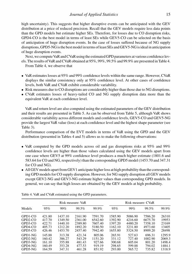
Next, we computeVaR and CVaR using the estimated GPD parameters at various confidence lev-els. The results ofVaR and CVaR obtained at 95%, 99%, 99.5% and 99.9% are presented in Table 4.

From Table 4, we observe that

• VaR estimates losses at 95% and 99% confidence levels within the same range. However, CVaRdisplays the similar consistency only at 95% confidence level. At other cases of confidencelevels, both VaR and CVaR exhibit considerable variability.

• Risk measures due to CO disruptions are considerably higher than those due to NG disruptions.• CVaR estimates losses of heavy-tailed CO and NG supply disruption data more than the

equivalent VaR at each confidence level.

VaR and return level are also computed using the estimated parameters of the GEV distributionand their results are presented in Table 5. As can be observed from Table 5, although VaR showsconsiderable variability across different models and confidence levels, GEV5-CO and GEV5-NGprovide the largest VaR value (loss) at each confidence level and the highest shape parameter (seeTable 3).

Performance comparison of the EVT models in terms of VaR using the GPD and the GEVdistribution (presented in Tables 4 and 5) allows us to make the following observations:

• VaR computed by the GPD models across oil and gas disruptions risks at 95% and 99%confidence levels are higher than those values calculated using the GEV models apart fromone case where GEV5 at 99% confidence level produces a much higher estimate (1801.6 and583.64 for CO and NG, respectively) than the corresponding GPD5 model (1453.70 and 347.31for CO and NG).

• All GEV models apart from GEV1 anticipate higher loss at high probability than the correspond-ing GPD models for CO supply disruption. However, for NG supply disruption all GEV modelsexcept GEV2-NG and GEV3-NG estimate higher values than corresponding GPD models. Ingeneral, we can say that high losses are obtained by the GEV models at high probability.

Table 4. VaR and CVaR estimated using the GPD parameters.

Risk measure: VaR Risk measure: CVaR

Models 95% 99% 99.5% 99.9% 95% 99% 99.5% 99.9%

GPD1-CO 421.80 1437.10 2161.90 7591.70 1585.90 5086.90 7586.20 26310GPD2-CO 417.70 1349.50 2361.00 6542.60 1392.90 4216.60 6675.70 19953GPD3-CO 422.71 1440.10 2389.80 7607.40 1397.20 4480.20 7358.10 23169GPD4-CO 405.73 1212.20 1892.20 5180.50 1162.10 3231.80 4973.60 13405GPD5-CO 426.46 1453.70 2457.40 7942.40 1655.80 5324.50 8909.20 28498GPD1-NG 145.88 313.38 421.34 805.06 265.91 527.63 696.31 1295.9GPD2-NG 160.42 386.27 543.29 1151.20 331.12 727.40 1002.90 2069.3GPD3-NG 161.10 355.88 481.43 927.66 300.68 605.04 801.20 1498.4GPD4-NG 160.49 353.28 477.53 919.19 298.65 599.88 794.02 1484.1GPD5-NG 164.59 347.31 461.28 851.92 293.00 565.72 735.82 1318.9


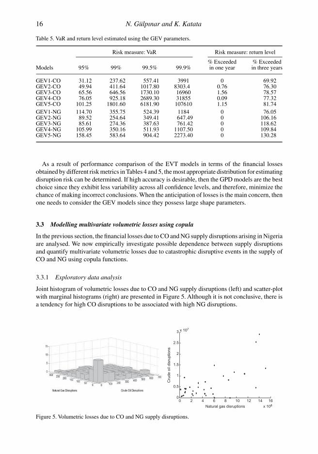
Table 5. VaR and return level estimated using the GEV parameters.

Risk measure: VaR Risk measure: return level

% Exceeded % ExceededModels 95% 99% 99.5% 99.9% in one year in three years

GEV1-CO 31.12 237.62 557.41 3991 0 69.92GEV2-CO 49.94 411.64 1017.80 8303.4 0.76 76.30GEV3-CO 65.56 646.56 1730.10 16960 1.56 78.57GEV4-CO 76.05 925.18 2689.30 31855 0.09 77.32GEV5-CO 101.25 1801.60 6181.90 107610 1.15 81.74GEV1-NG 114.70 355.75 524.39 1184 0 76.05GEV2-NG 89.52 254.64 349.41 647.49 0 106.16GEV3-NG 85.61 274.36 387.63 761.42 0 118.62GEV4-NG 105.99 350.16 511.93 1107.50 0 109.84GEV5-NG 158.45 583.64 904.42 2273.40 0 130.28

As a result of performance comparison of the EVT models in terms of the financial lossesobtained by different risk metrics in Tables 4 and 5, the most appropriate distribution for estimatingdisruption risk can be determined. If high accuracy is desirable, then the GPD models are the bestchoice since they exhibit less variability across all confidence levels, and therefore, minimize thechance of making incorrect conclusions. When the anticipation of losses is the main concern, thenone needs to consider the GEV models since they possess large shape parameters.

3.3 Modelling multivariate volumetric losses using copula

In the previous section, the financial losses due to CO and NG supply disruptions arising in Nigeriaare analysed. We now empirically investigate possible dependence between supply disruptionsand quantify multivariate volumetric losses due to catastrophic disruptive events in the supply ofCO and NG using copula functions.

3.3.1 Exploratory data analysis

Joint histogram of volumetric losses due to CO and NG supply disruptions (left) and scatter-plotwith marginal histograms (right) are presented in Figure 5. Although it is not conclusive, there isa tendency for high CO disruptions to be associated with high NG disruptions.

0 2 4 6 8 10 12 14 160

0.5

1

1.5

2

2.5

3 x 107

x 108Natural gas disruptions

Cru

de o

il di

srup

tions

Figure 5. Volumetric losses due to CO and NG supply disruptions.


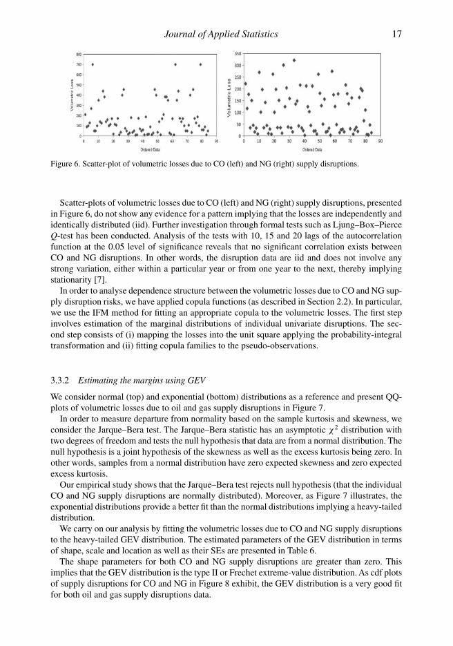
Figure 6. Scatter-plot of volumetric losses due to CO (left) and NG (right) supply disruptions.

Scatter-plots of volumetric losses due to CO (left) and NG (right) supply disruptions, presentedin Figure 6, do not show any evidence for a pattern implying that the losses are independently andidentically distributed (iid). Further investigation through formal tests such as Ljung–Box–PierceQ-test has been conducted. Analysis of the tests with 10, 15 and 20 lags of the autocorrelationfunction at the 0.05 level of significance reveals that no significant correlation exists betweenCO and NG disruptions. In other words, the disruption data are iid and does not involve anystrong variation, either within a particular year or from one year to the next, thereby implyingstationarity [7].

In order to analyse dependence structure between the volumetric losses due to CO and NG sup-ply disruption risks, we have applied copula functions (as described in Section 2.2). In particular,we use the IFM method for fitting an appropriate copula to the volumetric losses. The first stepinvolves estimation of the marginal distributions of individual univariate disruptions. The sec-ond step consists of (i) mapping the losses into the unit square applying the probability-integraltransformation and (ii) fitting copula families to the pseudo-observations.

3.3.2 Estimating the margins using GEV

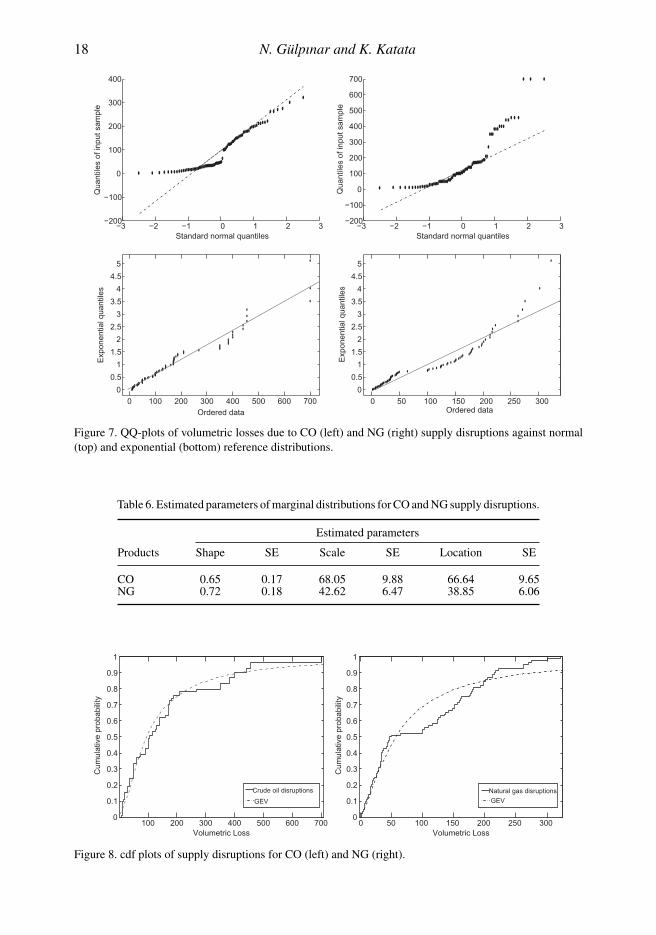
We consider normal (top) and exponential (bottom) distributions as a reference and present QQ-plots of volumetric losses due to oil and gas supply disruptions in Figure 7.

In order to measure departure from normality based on the sample kurtosis and skewness, weconsider the Jarque–Bera test. The Jarque–Bera statistic has an asymptotic χ2 distribution withtwo degrees of freedom and tests the null hypothesis that data are from a normal distribution. Thenull hypothesis is a joint hypothesis of the skewness as well as the excess kurtosis being zero. Inother words, samples from a normal distribution have zero expected skewness and zero expectedexcess kurtosis.

Our empirical study shows that the Jarque–Bera test rejects null hypothesis (that the individualCO and NG supply disruptions are normally distributed). Moreover, as Figure 7 illustrates, theexponential distributions provide a better fit than the normal distributions implying a heavy-taileddistribution.

We carry on our analysis by fitting the volumetric losses due to CO and NG supply disruptionsto the heavy-tailed GEV distribution. The estimated parameters of the GEV distribution in termsof shape, scale and location as well as their SEs are presented in Table 6.

The shape parameters for both CO and NG supply disruptions are greater than zero. Thisimplies that the GEV distribution is the type II or Frechet extreme-value distribution. As cdf plotsof supply disruptions for CO and NG in Figure 8 exhibit, the GEV distribution is a very good fitfor both oil and gas supply disruptions data.


−3 −2 −1 0 1 2 3−200

−100

0

100

200

300

400

Standard normal quantiles−3 −2 −1 0 1 2 3

Standard normal quantiles

Qua

ntile

s of

inpu

t sam

ple

−200

−100

0

100

200

300

400

500

600

700

Qua

ntile

s of

inpu

t sam

ple

0 100 200 300 400 500 600 700

0

0.5

1

1.5

2

2.5

3

3.5

4

4.5

5

Exp

onen

tial q

uant

iles

Ordered data0 50 100 150 200 250 300

0

0.5

1

1.5

2

2.5

3

3.5

4

4.5

5

Exp

onen

tial q

uant

iles

Ordered data

Figure 7. QQ-plots of volumetric losses due to CO (left) and NG (right) supply disruptions against normal(top) and exponential (bottom) reference distributions.

Table 6. Estimated parameters of marginal distributions for CO and NG supply disruptions.


Products Shape SE Scale SE Location SE

CO 0.65 0.17 68.05 9.88 66.64 9.65NG 0.72 0.18 42.62 6.47 38.85 6.06

100 200 300 400 500 600 7000

0.1

0.2

0.3

0.4

0.5

0.6

0.7

0.8

0.9

1

Volumetric Loss

Cum

ulat

ive

prob

abili

ty

0

0.1

0.2

0.3

0.4

0.5

0.6

0.7

0.8

0.9

1

Cum

ulat

ive

prob

abili

ty

Crude oil disruptions

GEV

0 50 100 150 200 250 300Volumetric Loss

Natural gas disruptions

GEV

Figure 8. cdf plots of supply disruptions for CO (left) and NG (right).


0 2 4 6 8 10 12 14 16x 108

0

0.5

1

1.5

2

2.5

3 x 107


Cru

de O

il di

srup

tions

0.1 0.2 0.3 0.4 0.5 0.6 0.7 0.8 0.9 10

0.1

0.2

0.3

0.4

0.5

0.6

0.7

0.8

0.9

1


Cru

de o

il di

srup

tions

Figure 9. Scatter-plots of supply disruptions (left) and the pseudo-observations (right).

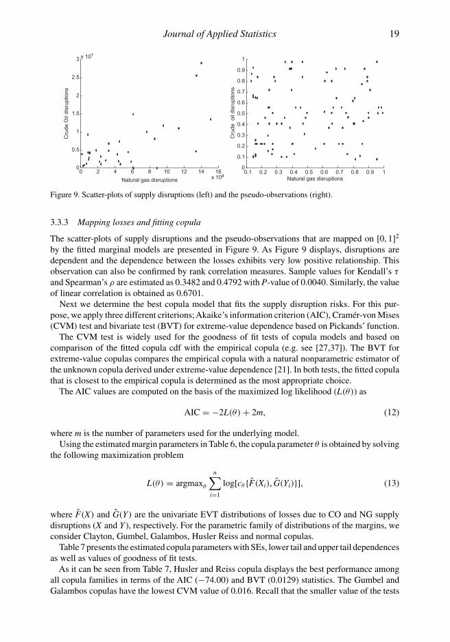
3.3.3 Mapping losses and fitting copula

The scatter-plots of supply disruptions and the pseudo-observations that are mapped on [0, 1]2

by the fitted marginal models are presented in Figure 9. As Figure 9 displays, disruptions aredependent and the dependence between the losses exhibits very low positive relationship. Thisobservation can also be confirmed by rank correlation measures. Sample values for Kendall’s τ

and Spearman’s ρ are estimated as 0.3482 and 0.4792 with P-value of 0.0040. Similarly, the valueof linear correlation is obtained as 0.6701.

Next we determine the best copula model that fits the supply disruption risks. For this pur-pose, we apply three different criterions; Akaike’s information criterion (AIC), Cramér-von Mises(CVM) test and bivariate test (BVT) for extreme-value dependence based on Pickands’ function.

The CVM test is widely used for the goodness of fit tests of copula models and based oncomparison of the fitted copula cdf with the empirical copula (e.g. see [27,37]). The BVT forextreme-value copulas compares the empirical copula with a natural nonparametric estimator ofthe unknown copula derived under extreme-value dependence [21]. In both tests, the fitted copulathat is closest to the empirical copula is determined as the most appropriate choice.

The AIC values are computed on the basis of the maximized log likelihood (L(θ)) as

AIC = −2L(θ) + 2m, (12)

where m is the number of parameters used for the underlying model.Using the estimated margin parameters in Table 6, the copula parameter θ is obtained by solving

the following maximization problem

L(θ) = argmaxθ

n∑i=1

log[cθ {F(Xi), G(Yi)}], (13)

where F(X) and G(Y) are the univariate EVT distributions of losses due to CO and NG supplydisruptions (X and Y ), respectively. For the parametric family of distributions of the margins, weconsider Clayton, Gumbel, Galambos, Husler Reiss and normal copulas.

Table 7 presents the estimated copula parameters with SEs, lower tail and upper tail dependencesas well as values of goodness of fit tests.

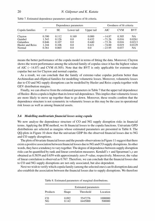
As it can be seen from Table 7, Husler and Reiss copula displays the best performance amongall copula families in terms of the AIC (−74.00) and BVT (0.0129) statistics. The Gumbel andGalambos copulas have the lowest CVM value of 0.016. Recall that the smaller value of the tests


Table 7. Estimated dependence parameters and goodness of fit criteria.

Dependence parameters Goodness of fit criteria

Copula families θ SE Lower tail Upper tail AIC CVM BVT

Clayton 0.390 0.112 0.169 0.000 −14.87 0.305 NAGumbel 1.543 0.126 0.0 0.432 −71.26 0.016 0.0261Galambos 0.846 0.107 0.0 0.440 −73.36 0.016 0.0213Husler and Reiss 1.244 0.106 0.0 0.421 −74.00 0.019 0.0129Normal 0.361 0.065 0.0 0.0 −23.95 0.037 NA

means the better performance of the copula model in terms of fitting the data. Moreover, Claytonshows the worst performance among the selected family of copulas since it has the highest valuesof AIC (−14.87) and CVM (0.305). Note that the BVT is only applicable for extreme-valuecopulas but not for Clayton and normal copulas.

As a result, we can conclude that the family of extreme-value copulas perform better thanArchimedian and elliptical families for modelling volumetric losses. Moreover, volumetric lossesdue to CO and NG supply disruptions can be modelled by Husler and Reiss copula together withGEV distribution margins.

Finally, we can observe from the estimated parameters in Table 7 that the upper tail dependenceof Huslee–Reiss copula is higher than its lower tail dependence. This implies that volumetric lossesare more likely to move up together than to go down. Moreover, these results confirm that thedependence structure is not symmetric in volumetric losses as this may be the case in operationalrisk losses as well as among financial assets.

3.4 Modelling multivariate financial losses using copula

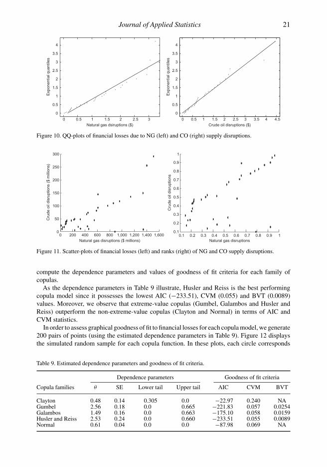
We now analyse the dependence structure of CO and NG supply disruption risks in financialterms. Applying the IFM method, we fit financial losses to the copula functions. Univariate GPDdistributions are selected as margins whose estimated parameters are presented in Table 8. TheQQ-plots in Figure 10 show that the univariate GDP fits the observed financial losses due to NGand CO supply disruptions.

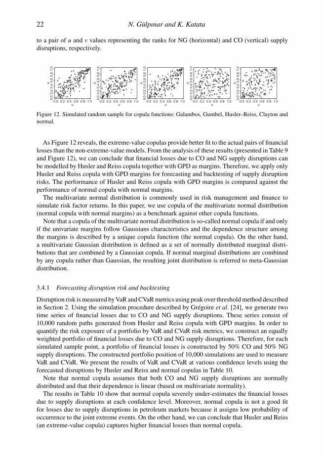
The plots of bivariate financial losses and the pseudo-observations in Figure 11 suggest that thereexists a positive association between financial losses due to NG and CO supply disruptions. In otherwords, they have a tendency to vary together. The degree of dependence between supply disruptionrisks can be quantified by rank and linear correlation measures. Kendall’s τ and Spearman’s ρ areobtained as 0.5839 and 0.659 with approximately zero P-value, respectively. Moreover, the valueof linear correlation is observed as 0.767. Therefore, we can conclude that the financial losses dueto CO and NG supply disruptions are not only associated, but also dependent.

Next we wish to verify which copula family (among the selected ones) can fit disruption data andalso establish the association between the financial losses due to supply disruptions. We therefore

Table 8. Estimated parameters of marginal distributions.


Products Shape Threshold Location

CO 0.092 5547276 1000000NG 0.142 6445000 500000


0 0.5 1 1.5 2 2.5 3

0

0.5

1

1.5

2

2.5

3

3.5

4E

xpon

entia

l qua

ntile

s

Natural gas dsiruptions ($)

0 0.5 1 1.5 2 2.5 3 3.5 4 4.5

0

0.5

1

1.5

2

2.5

3

3.5

4

Exp

onen

tial q

uant

iles

Crude oil disruptions ($)

Figure 10. QQ-plots of financial losses due to NG (left) and CO (right) supply disruptions.

0 200 400 600 800 1,000 1,200 1,400 1,6000

50

100

150

200

250

300

Natural gas disruptions ($ millions)

Cru

de o

il di

srup

tions

($

mill

ions

)

0.1 0.2 0.3 0.4 0.5 0.6 0.7 0.8 0.9 10.1

0.2

0.3

0.4

0.5

0.6

0.7

0.8

0.9

1


Cru

de o

il di

srup

tions

Figure 11. Scatter-plots of financial losses (left) and ranks (right) of NG and CO supply disruptions.

compute the dependence parameters and values of goodness of fit criteria for each family ofcopulas.

As the dependence parameters in Table 9 illustrate, Husler and Reiss is the best performingcopula model since it possesses the lowest AIC (−233.51), CVM (0.055) and BVT (0.0089)values. Moreover, we observe that extreme-value copulas (Gumbel, Galambos and Husler andReiss) outperform the non-extreme-value copulas (Clayton and Normal) in terms of AIC andCVM statistics.

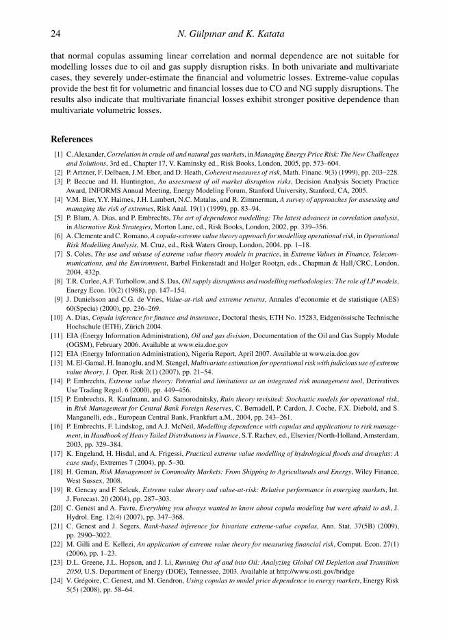
In order to assess graphical goodness of fit to financial losses for each copula model, we generate200 pairs of points (using the estimated dependence parameters in Table 9). Figure 12 displaysthe simulated random sample for each copula function. In these plots, each circle corresponds

Table 9. Estimated dependence parameters and goodness of fit criteria.

Dependence parameters Goodness of fit criteria

Copula families θ SE Lower tail Upper tail AIC CVM BVT

Clayton 0.48 0.14 0.305 0.0 −22.97 0.240 NAGumbel 2.56 0.18 0.0 0.665 −221.83 0.057 0.0254Galambos 1.49 0.16 0.0 0.663 −175.10 0.058 0.0159Husler and Reiss 2.53 0.24 0.0 0.660 −233.51 0.055 0.0089Normal 0.61 0.04 0.0 0.0 −87.98 0.069 NA


to a pair of u and v values representing the ranks for NG (horizontal) and CO (vertical) supplydisruptions, respectively.

u

v v v v v

0.0

0.2

0.4

0.6

0.8

1.0

0.0 0.2 0.4 0.6 0.8 1.0u

0.0 0.2 0.4 0.6 0.8 1.0u

0.0 0.2 0.4 0.6 0.8 1.0u

0.0 0.2 0.4 0.6 0.8 1.0u

0.0 0.2 0.4 0.6 0.8 1.00.

00.

20.

40.

60.

81.

0

0.0

0.2

0.4

0.6

0.8

1.0

0.0

0.2

0.4

0.6

0.8

1.0

v0.

00.

20.

40.

60.

81.

0

Figure 12. Simulated random sample for copula functions: Galambos, Gumbel, Husler–Reiss, Clayton andnormal.

As Figure 12 reveals, the extreme-value copulas provide better fit to the actual pairs of financiallosses than the non-extreme-value models. From the analysis of these results (presented in Table 9and Figure 12), we can conclude that financial losses due to CO and NG supply disruptions canbe modelled by Husler and Reiss copula together with GPD as margins. Therefore, we apply onlyHusler and Reiss copula with GPD margins for forecasting and backtesting of supply disruptionrisks. The performance of Husler and Reiss copula with GPD margins is compared against theperformance of normal copula with normal margins.

The multivariate normal distribution is commonly used in risk management and finance tosimulate risk factor returns. In this paper, we use copula of the multivariate normal distribution(normal copula with normal margins) as a benchmark against other copula functions.

Note that a copula of the multivariate normal distribution is so-called normal copula if and onlyif the univariate margins follow Gaussians characteristics and the dependence structure amongthe margins is described by a unique copula function (the normal copula). On the other hand,a multivariate Gaussian distribution is defined as a set of normally distributed marginal distri-butions that are combined by a Gaussian copula. If normal marginal distributions are combinedby any copula rather than Gaussian, the resulting joint distribution is referred to meta-Gaussiandistribution.

3.4.1 Forecasting disruption risk and backtesting

Disruption risk is measured byVaR and CVaR metrics using peak over threshold method describedin Section 2. Using the simulation procedure described by Grégoire et al. [24], we generate twotime series of financial losses due to CO and NG supply disruptions. These series consist of10,000 random paths generated from Husler and Reiss copula with GPD margins. In order toquantify the risk exposure of a portfolio by VaR and CVaR risk metrics, we construct an equallyweighted portfolio of financial losses due to CO and NG supply disruptions. Therefore, for eachsimulated sample point, a portfolio of financial losses is constructed by 50% CO and 50% NGsupply disruptions. The constructed portfolio position of 10,000 simulations are used to measureVaR and CVaR. We present the results of VaR and CVaR at various confidence levels using theforecasted disruptions by Husler and Reiss and normal copulas in Table 10.

Note that normal copula assumes that both CO and NG supply disruptions are normallydistributed and that their dependence is linear (based on multivariate normality).

The results in Table 10 show that normal copula severely under-estimates the financial lossesdue to supply disruptions at each confidence level. Moreover, normal copula is not a good fitfor losses due to supply disruptions in petroleum markets because it assigns low probability ofoccurrence to the joint extreme events. On the other hand, we can conclude that Husler and Reiss(an extreme-value copula) captures higher financial losses than normal copula.


Table 10. Simulated risk measures using fitted and normal copula functions.

Models Confidence level (%) VaR (1000s) CVaR (1000s)

Husler and Reiss copula 95.0 165430 236740with GPD margins 99.0 277070 362650

99.5 331790 42436099.9 476710 587800

Normal copula 95.0 16863 20319with normal margins 99.0 22558 25164

99.5 24557 2686599.9 28361 30102

Figure 13. Backtesting of a portfolio comprising losses due to CO and NG supply disruptions.

In order to asses the accuracy of disruption risk measured by VaR and CVaR, we conduct abacktest using Husler and Reiss copula model with GPD margins at various confidence levels.We follow a rolling window of 500 observations out of the sample. We estimate risk measureswith 10,000 observations and move by a window of 500 observations. At each observation point,we delete the 500 oldest bivariate disruption losses after moving the data by 500 places to the501st observation and re-estimate VaR and CVaR. Figure 13 presents the result of backtesting at99.9% confidence levels. As Figure 13 illustrates, there are only 3 and 5 losses that exceed CVaRand VaR, respectively. Therefore, we can conclude that the forecasted CVaR and VaR measuresare adequate in capturing the financial losses due to CO and NG supply disruptions. Backtestingresults at various confidence levels also confirm this observation.

4. Conclusions

In this paper, we model oil and gas supply disruption risks using EVT and various copula functions.In order to empirically investigate the performance of these models, we consider Nigeria as a casestudy. The EVT models are used to describe univariate CO and NG supply disruption risks interms of volumetric and financial losses. The copula functions model the probability of occurrenceand multivariate dependence between CO and NG supply disruptions.

Our empirical analysis reveals that losses due to CO disruptions have more significant negativeimpact than losses due to NG disruption risks in Nigeria. Moreover, the GEV models can anticipatehigher financial losses while the GPD models can produce more accurate results. We also observe


that normal copulas assuming linear correlation and normal dependence are not suitable formodelling losses due to oil and gas supply disruption risks. In both univariate and multivariatecases, they severely under-estimate the financial and volumetric losses. Extreme-value copulasprovide the best fit for volumetric and financial losses due to CO and NG supply disruptions. Theresults also indicate that multivariate financial losses exhibit stronger positive dependence thanmultivariate volumetric losses.

References

[1] C.Alexander, Correlation in crude oil and natural gas markets, in Managing Energy Price Risk: The New Challengesand Solutions, 3rd ed., Chapter 17, V. Kaminsky ed., Risk Books, London, 2005, pp. 573–604.

[2] P. Artzner, F. Delbaen, J.M. Eber, and D. Heath, Coherent measures of risk, Math. Financ. 9(3) (1999), pp. 203–228.[3] P. Beccue and H. Huntington, An assessment of oil market disruption risks, Decision Analysis Society Practice

Award, INFORMS Annual Meeting, Energy Modeling Forum, Stanford University, Stanford, CA, 2005.[4] V.M. Bier, Y.Y. Haimes, J.H. Lambert, N.C. Matalas, and R. Zimmerman, A survey of approaches for assessing and

managing the risk of extremes, Risk Anal. 19(1) (1999), pp. 83–94.[5] P. Blum, A. Dias, and P. Embrechts, The art of dependence modelling: The latest advances in correlation analysis,

in Alternative Risk Strategies, Morton Lane, ed., Risk Books, London, 2002, pp. 339–356.[6] A. Clemente and C. Romano, A copula-extreme value theory approach for modelling operational risk, in Operational

Risk Modelling Analysis, M. Cruz, ed., Risk Waters Group, London, 2004, pp. 1–18.[7] S. Coles, The use and misuse of extreme value theory models in practice, in Extreme Values in Finance, Telecom-

munications, and the Environment, Barbel Finkenstadt and Holger Rootzn, eds., Chapman & Hall/CRC, London,2004, 432p.

[8] T.R. Curlee, A.F. Turhollow, and S. Das, Oil supply disruptions and modelling methodologies: The role of LP models,Energy Econ. 10(2) (1988), pp. 147–154.

[9] J. Danielsson and C.G. de Vries, Value-at-risk and extreme returns, Annales d’economie et de statistique (AES)60(Specia) (2000), pp. 236–269.

[10] A. Dias, Copula inference for finance and insurance, Doctoral thesis, ETH No. 15283, Eidgenössische TechnischeHochschule (ETH), Zürich 2004.

[11] EIA (Energy Information Administration), Oil and gas division, Documentation of the Oil and Gas Supply Module(OGSM), February 2006. Available at www.eia.doe.gov

[12] EIA (Energy Information Administration), Nigeria Report, April 2007. Available at www.eia.doe.gov[13] M. El-Gamal, H. Inanoglu, and M. Stengel, Multivariate estimation for operational risk with judicious use of extreme

value theory, J. Oper. Risk 2(1) (2007), pp. 21–54.[14] P. Embrechts, Extreme value theory: Potential and limitations as an integrated risk management tool, Derivatives

Use Trading Regul. 6 (2000), pp. 449–456.[15] P. Embrechts, R. Kaufmann, and G. Samorodnitsky, Ruin theory revisited: Stochastic models for operational risk,

in Risk Management for Central Bank Foreign Reserves, C. Bernadell, P. Cardon, J. Coche, F.X. Diebold, and S.Manganelli, eds., European Central Bank, Frankfurt a.M., 2004, pp. 243–261.

[16] P. Embrechts, F. Lindskog, and A.J. McNeil, Modelling dependence with copulas and applications to risk manage-ment, in Handbook of Heavy Tailed Distributions in Finance, S.T. Rachev, ed., Elsevier/North-Holland, Amsterdam,2003, pp. 329–384.

[17] K. Engeland, H. Hisdal, and A. Frigessi, Practical extreme value modelling of hydrological floods and droughts: Acase study, Extremes 7 (2004), pp. 5–30.

[18] H. Geman, Risk Management in Commodity Markets: From Shipping to Agriculturals and Energy, Wiley Finance,West Sussex, 2008.

[19] R. Gencay and F. Selcuk, Extreme value theory and value-at-risk: Relative performance in emerging markets, Int.J. Forecast. 20 (2004), pp. 287–303.

[20] C. Genest and A. Favre, Everything you always wanted to know about copula modeling but were afraid to ask, J.Hydrol. Eng. 12(4) (2007), pp. 347–368.

[21] C. Genest and J. Segers, Rank-based inference for bivariate extreme-value copulas, Ann. Stat. 37(5B) (2009),pp. 2990–3022.

[22] M. Gilli and E. Kellezi, An application of extreme value theory for measuring financial risk, Comput. Econ. 27(1)(2006), pp. 1–23.

[23] D.L. Greene, J.L. Hopson, and J. Li, Running Out of and into Oil: Analyzing Global Oil Depletion and Transition2050, U.S. Department of Energy (DOE), Tennessee, 2003. Available at http://www.osti.gov/bridge

[24] V. Grégoire, C. Genest, and M. Gendron, Using copulas to model price dependence in energy markets, Energy Risk5(5) (2008), pp. 58–64.

http://www.osti.gov/bridge


[25] P. Grossi and H. Kunreuther, Catastrophe Modelling: A New Approach to Managing Risk, Springer, NewYork, 2005.[26] P.R. Kleindorfer and G.H. Saad, Disruption risk management in supply chains, Prod. Oper. Manage. 14(1) (2005),

pp. 53–68.[27] E. Kole, K. Koedijk, and M. Verbeek, Selecting copulas for risk management, J. Bank. Financ. 31 (2007), pp. 2405–

2423.[28] L. Kumins and R. Bamberger, Oil and gas disruption from Hurricanes Katrina and Rita, CRS Rep. for Congress,

Order Code RL33124, Congressional Research Service, The Library of Congress, Washington, 2006.[29] V. Marimoutoua, B. Raggadb, and A. Trabelsib, Extreme value theory and value at risk: Application to oil market,

Energy Econ. 31 (2009), pp. 519–530.[30] A.J. McNeil, Estimating the tails of loss severity distributions using extreme value theory, ASTIN Bull. 27 (1997),

pp. 117–137.[31] A.J. McNeil and R. Frey, Estimation of tail-related risk measures for heteroscedastic financial time series: An extreme

value approach, J. Empir. Financ. 7 (2000), pp. 271–300.[32] A.J. McNeil, R. Frey, and P. Embrechts, Quantitative Risk Management: Concepts, Techniques, and Tools, Princeton

University Press, Princeton, 2005.[33] A.J. McNeil and T. Saladin, The peaks over thresholds method for estimating high quantiles of loss distributions,

Proceedings of 28th International ASTIN Colloquium, Cairns, Australia, 1997.[34] A. Meela, L.M. O’Neilla, J.H. Levina, W.D. Seidera, U. Oktemb, and N. Kerenc, Operational risk assessment of

chemical industries by exploiting accident databases, J. Loss Prevention Process Ind. 20 (2007), pp. 113–127.[35] H. Mohtadi and A. Murshid, The risk of catastrophic terrorism: An extreme value approach, J. Appl. Econ. 24(4)

(2009), pp. 537–559.[36] R. Nelsen, An Introduction to Copulas, Springer Science and Business Media, Inc., New York, 2006.[37] A. Patton, Copula methods for forecasting multivariate time series, 2012, in Handbook of Economic Forecasting 2,

G. Elliott and A. Timmermann, eds., Springer Verlag, New York, 2012.[38] J. Rank, Copulas from Theory to Application in Finance, Risk Books, London, 2007.[39] D.B. Reister, A compact model of oil supply disruptions, Resour. Energy 10 (1988), pp. 161–183.[40] F. Ren and D.E. Giles, Extreme value analysis of daily Canadian crude oil prices, Econometrics Working Paper

EWP0708, Department of Economics, University of Victoria, Victoria, 2007.[41] T. Schmidt, Coping with copulas, in Copulas From Theory to Application in Finance, J. Rank, ed., Risk Books,

London, 2007.

Copyright of Journal of Applied Statistics is the property of Routledge and its content maynot be copied or emailed to multiple sites or posted to a listserv without the copyright holder'sexpress written permission. However, users may print, download, or email articles forindividual use.

Documents

ContentServer.asp 2