Embed Size (px)
Citation preview
Contents
1 APERITIFS 7
1.1 Diffusion . . . . . . . . . . . . . . . . . . . . . . . . . . . . . . . . . . . . . . . . . . . . . . . . 7
1.2 Single-Species Annihilation . . . . . . . . . . . . . . . . . . . . . . . . . . . . . . . . . . . . . 9
1.3 Two-Species Annihilation . . . . . . . . . . . . . . . . . . . . . . . . . . . . . . . . . . . . . . 12
2 RANDOM WALK/DIFFUSION 17
2.1 Langevin Equation . . . . . . . . . . . . . . . . . . . . . . . . . . . . . . . . . . . . . . . . . . 17
2.2 Master Equation for the Probability Distribution . . . . . . . . . . . . . . . . . . . . . . . . . 18
2.3 Connection to First-Passage Properties . . . . . . . . . . . . . . . . . . . . . . . . . . . . . . . 21
3 AGGREGATION 27
3.1 Exact Solutions . . . . . . . . . . . . . . . . . . . . . . . . . . . . . . . . . . . . . . . . . . . . 28
3.2 Theory of the Reaction Rate . . . . . . . . . . . . . . . . . . . . . . . . . . . . . . . . . . . . 37
3.3 Scaling Theory . . . . . . . . . . . . . . . . . . . . . . . . . . . . . . . . . . . . . . . . . . . . 40
3.4 Extensions . . . . . . . . . . . . . . . . . . . . . . . . . . . . . . . . . . . . . . . . . . . . . . . 41
3.4.1 Exchange . . . . . . . . . . . . . . . . . . . . . . . . . . . . . . . . . . . . . . . . . . . 41
3.4.2 Aggregation with Input . . . . . . . . . . . . . . . . . . . . . . . . . . . . . . . . . . . 43
3.4.3 Finite Systems . . . . . . . . . . . . . . . . . . . . . . . . . . . . . . . . . . . . . . . . 45
4 FRAGMENTATION 49
4.1 Exact Solutions . . . . . . . . . . . . . . . . . . . . . . . . . . . . . . . . . . . . . . . . . . . . 50
4.2 Scaling Theory . . . . . . . . . . . . . . . . . . . . . . . . . . . . . . . . . . . . . . . . . . . . 53
4.3 The Shattering Transition . . . . . . . . . . . . . . . . . . . . . . . . . . . . . . . . . . . . . . 56
4.4 Fragmentation with Input . . . . . . . . . . . . . . . . . . . . . . . . . . . . . . . . . . . . . . 57
4.5 Geometrical Fragmentation . . . . . . . . . . . . . . . . . . . . . . . . . . . . . . . . . . . . . 59
5 ADSORPTION 63
5.1 Random Sequential Adsorption . . . . . . . . . . . . . . . . . . . . . . . . . . . . . . . . . . . 63
5.2 Adsorption-diffusion and reaction equivalence . . . . . . . . . . . . . . . . . . . . . . . . . . . 78
5.3 Adsorption-Desorption and slow dynamics . . . . . . . . . . . . . . . . . . . . . . . . . . . . . 79
5.4 Cooperative sequential adsorption . . . . . . . . . . . . . . . . . . . . . . . . . . . . . . . . . 82
5.5 Nucleation and growth . . . . . . . . . . . . . . . . . . . . . . . . . . . . . . . . . . . . . . . . 85
6 SPIN DYNAMICS 91
6.1 Glauber Spin-Flip Dynamics . . . . . . . . . . . . . . . . . . . . . . . . . . . . . . . . . . . . 91
6.2 Kawasaki spin-exchange dynamics . . . . . . . . . . . . . . . . . . . . . . . . . . . . . . . . . 99
6.3 Cluster dynamics . . . . . . . . . . . . . . . . . . . . . . . . . . . . . . . . . . . . . . . . . . . 101
6.4 Extremal dynamics . . . . . . . . . . . . . . . . . . . . . . . . . . . . . . . . . . . . . . . . . . 104
6.5 Voter Model . . . . . . . . . . . . . . . . . . . . . . . . . . . . . . . . . . . . . . . . . . . . . . 108
6.6 Disordered Spin Chains . . . . . . . . . . . . . . . . . . . . . . . . . . . . . . . . . . . . . . . 112
6.7 Disordered Systems . . . . . . . . . . . . . . . . . . . . . . . . . . . . . . . . . . . . . . . . . . 118
1

2 CONTENTS
7 ANOMALOUS TRANSPORT 1217.1 The Asymmetric Exclusion Process . . . . . . . . . . . . . . . . . . . . . . . . . . . . . . . . . 1217.2 Random Walks in Random Environments . . . . . . . . . . . . . . . . . . . . . . . . . . . . . 1267.3 Random Walks in Random Velocity Fields . . . . . . . . . . . . . . . . . . . . . . . . . . . . . 130
8 HYSTERESIS 1338.1 Homogeneous Ferromagnets . . . . . . . . . . . . . . . . . . . . . . . . . . . . . . . . . . . . . 1338.2 Disordered Ferromagnets . . . . . . . . . . . . . . . . . . . . . . . . . . . . . . . . . . . . . . . 141
9 REACTIONS 1519.1 Single-Species . . . . . . . . . . . . . . . . . . . . . . . . . . . . . . . . . . . . . . . . . . . . . 1519.2 Two Species Annihilation . . . . . . . . . . . . . . . . . . . . . . . . . . . . . . . . . . . . . . 1599.3 The Trapping Reaction . . . . . . . . . . . . . . . . . . . . . . . . . . . . . . . . . . . . . . . 163
9.3.1 Exact Solution in One Dimension . . . . . . . . . . . . . . . . . . . . . . . . . . . . . . 1649.3.2 Lifshitz Argument for General Spatial Dimension . . . . . . . . . . . . . . . . . . . . . 166
10 COARSENING 17110.1 The Models . . . . . . . . . . . . . . . . . . . . . . . . . . . . . . . . . . . . . . . . . . . . . . 17110.2 Scaling . . . . . . . . . . . . . . . . . . . . . . . . . . . . . . . . . . . . . . . . . . . . . . . . . 17210.3 Non-conservative Dynamics . . . . . . . . . . . . . . . . . . . . . . . . . . . . . . . . . . . . . 174
11 COLLISIONS 18111.1 Inelastic Gases . . . . . . . . . . . . . . . . . . . . . . . . . . . . . . . . . . . . . . . . . . . . 18211.2 Lorentz Gas . . . . . . . . . . . . . . . . . . . . . . . . . . . . . . . . . . . . . . . . . . . . . . 19611.3 Traffic Flows . . . . . . . . . . . . . . . . . . . . . . . . . . . . . . . . . . . . . . . . . . . . . 19611.4 Sticky Gases . . . . . . . . . . . . . . . . . . . . . . . . . . . . . . . . . . . . . . . . . . . . . 20411.5 Ballistic Annihilation . . . . . . . . . . . . . . . . . . . . . . . . . . . . . . . . . . . . . . . . . 206
12 GROWING NETWORKS 20912.1 Models . . . . . . . . . . . . . . . . . . . . . . . . . . . . . . . . . . . . . . . . . . . . . . . . . 21012.2 Structure of the Growing Network . . . . . . . . . . . . . . . . . . . . . . . . . . . . . . . . . 21112.3 Global Properties . . . . . . . . . . . . . . . . . . . . . . . . . . . . . . . . . . . . . . . . . . . 215
13 REFERENCES 219
A MATTERS OF TECHNIQUE 229A.1 Transform Methods . . . . . . . . . . . . . . . . . . . . . . . . . . . . . . . . . . . . . . . . . . 229A.2 Relation between Laplace Transforms and Real Time Quantities . . . . . . . . . . . . . . . . 229A.3 Asymptotic Analysis . . . . . . . . . . . . . . . . . . . . . . . . . . . . . . . . . . . . . . . . . 232A.4 Scaling Approaches . . . . . . . . . . . . . . . . . . . . . . . . . . . . . . . . . . . . . . . . . . 232A.5 Differential Equations . . . . . . . . . . . . . . . . . . . . . . . . . . . . . . . . . . . . . . . . 232A.6 Partial Differential Equation . . . . . . . . . . . . . . . . . . . . . . . . . . . . . . . . . . . . . 234A.7 Extreme Statistics . . . . . . . . . . . . . . . . . . . . . . . . . . . . . . . . . . . . . . . . . . 234A.8 Probability theory . . . . . . . . . . . . . . . . . . . . . . . . . . . . . . . . . . . . . . . . . . 235
B Formulas & Distributions 237B.1 Useful Formulas . . . . . . . . . . . . . . . . . . . . . . . . . . . . . . . . . . . . . . . . . . . . 237

Preface
Statistical physics is an unusual branch of physics because it is not really a well-defined field in a formalsense, but rather, statistical physics is a viewpoint – indeed, the most appropriate viewpoint – to investigatesystems with many degrees of freedom. Part of the appeal of statistical physics is that it can be applied to adisparate range of systems that are in the mainstream of physics, as well as to problems that might appearto be outside physics, such as econophysics, quantitative biology, and social organization phenomena. Manyof the basic features of these systems involve fluctuations or explicit time evolution rather than equilibriumdistributions. Thus the approaches of non-equilibrium statistical physics are needed to discuss such systems.
While the tools of equilibrium statistical physics are well-developed, the statistical description of systemsthat are out of equilibrium is still relatively primitive. In spite of more than a century of effort in constructingan over-arching approach for non-equilibrium phenomena, there still does not exist canonical formulations,such as the Boltzmann factor or the partition function in equilibrium statistical physics. At the presenttime, some of the most important theoretical approaches for non-equilibrium systems are either technical,such as deriving hydrodynamics from the Boltzmann equation, or somewhat removed from the underlyingphenomena that are being described, such as non-equilibrium thermodynamics.
Because of this disconnect between fundamental theory and applications, our view is that it is moreinstructive to illustrate non-equilibrium statistical physics by presenting a number of current and paradig-matic examples of systems that are out of equilibrium, and to elucidate, as completely as possible, the rangeof techniques available to solve these systems. By this approach, we believe that readers can gain generalinsights more quickly compared to formal approaches, and, further, will be well-equipped to understandmany other topics in non-equilibrium statistical physics. We have attempted to make our treatment asself-contained and user-friendly as possible, so that an interested reader can work through the book withoutencountering unresolved methodological mysteries or hidden calculational pitfalls. Thus while much of thematerial is mathematical in nature, we have tried to present it as pedagogically as possible. Our targetaudience is graduate students with a one-course background in equilibrium statistical physics. Each of themain chapters is intended to be self-contained. We also made an effort to supplement the chapters withresearch exercises and open questions, in the hopes of stimulating further research.
The specific examples presented in this book are primarily based on irreversible stochastic processes. Thisbranch of statistical physics is in many ways the natural progression of kinetic theory that was initially usedto describe dynamics of simple gases and fluids. We will discuss the development of basic kinetic approachesto more complex and contemporary systems. Among the large menu of stochastic and irreversible processes,we chose the ones that we consider to be among the most important and most instructive in leading togeneric understanding. Our main emphasis is on exact analytical results, but we also send time developingheuristic and scaling methods. We largely avoid presenting numerical simulation results because these areless definitive and instructive than analytical results. An appealing (at least to us) aspect of these examplesis that they are broadly accessible. One needs little background to appreciate the systems being studied andthe ideas underlying the methods of solution. Many of these systems naturally suggest new and non-trivialquestions that an interested reader can easily pursue.
We begin our exposition with a few “aperitifs” – an abbreviated qualitative discussion of basic problemsand a general hint at the approaches that are available to solve these systems. Chapter 2 provides a basicintroduction to diffusion phenomena because of the central role played by diffusion in many non-equilibriumstatistical systems. These preliminary chapters serve as an introduction to the rest of the book.
The main body of the book is then devoted to working out specific examples. In the next three chapters,we discuss the fundamental kinetic processes of aggregation, fragmentation, and adsorption (chapters 3–5).
3

4 CONTENTS
Aggregation is the process by which two clusters irreversibly combine in a mass-conserving manner to form alarger cluster. This classic process that very nicely demonstrates the role of conservation laws, the utility ofexact solutions, the emergence of scaling in cluster-size distributions, and the power of heuristic derivations.Many of these technical lessons will be applied throughout this book.
We then turn to the complementary process of fragmentation, which involves the repeated breakup ofan element into smaller fragments. While this phenomenon again illustrates the utility of exact and scalingsolutions, fragmentation also exposes important new concepts such as multiscaling, lack of self-averaging, andmethods such as traveling waves and velocity selection. All of these are concepts that are used extensively innon-equilibrium statistical physics. We then discuss the phenomenon of irreversible adsorption where, again,the exact solutions of underlying master equations for the occupancy probability distributions provides acomprehensive picture of the basic phenomena.
The next two chapters (6 & 7) discuss the time evolution of systems that involve the competition betweenmultiple phases. We first treat classical spin systems, in particular, the kinetic Ising model and the votermodel. The kinetic Ising model occupies a central role in statistical physics because of its broad applicabilityto spins systems and many other dynamic critical phenomena. The voter model is perhaps not as well knownin the physics literature, but it is an even simpler model of an evolving spin system that is exactly solublein all dimensions. In chapter 7, we study phase ordering kinetics. Here the natural descriptions are in termsof continuum differential equations, rather than master equations.
In chapter 8, we discuss collision-driven phenomena. Our aim is to present the Boltzmann equation inthe context of explicitly soluble examples. These include traffic models, and aggregation and annihilationprocesses in which the particles move at constant velocity between collisions. The final chapter (#9) presentsseveral applications to contemporary problems, such as the structure of growing networks and models of self-organized criticality.
In an appendix, we present the fundamental techniques that are used throughout our book. Theseinclude various types of integral transforms, generating functions, asymptotic analysis, extreme statistics,and scaling approaches. Each of these methods is explain fully upon its first appearance in the book itself,and the appendix is a brief compendium of these methods that can be used either as a reference or a studyguide, depending on one’s technical preparation.

Chapter 1
APERITIFS
Broadly speaking, non-equilibrium statistical physics describes the time-dependent evolution of many-particlesystems. The individual particles are elemental interacting entities which, in some situations, can changein the process of interaction. In the most interesting cases, interactions between particles are strong andhence the deterministic description of even few-particle systems are beyond the reach of exact theoreticalapproaches. On the other hand, many-particle systems often admit an analytical statistical description whentheir number becomes large and in that sense they are simpler than few-particle systems. This feature hasseveral different names—the law of large numbers, ergodicity, etc.—and it is one of the reasons for thespectacular successes of statistical physics and probability theory.
Non-equilibrium statistical physics is quite different from other branches of physics, such as the ’fun-damental’ fields of electrodynamics, gravity, and elementary-particle physics that involve a reductionistdescription of few-particle systems, and applied fields, such as hydrodynamics and elasticity that are primar-ily concerned with the consequences of fundamental governing equations. Some of the key and distinguishingfeatures of non-equilibrium statistical physics include:
• no basic equations (like Maxwell equations in electrodynamics or Navier-Stokes equations in hydrody-namics) from which the rest follows;
• intermediate between fundamental applied physics;
• the existence of common underlying techniques and concepts in spite of the wide diversity of the field;
• non-equilibrium statistical physics naturally leads to the creation of methods that are quite useful inapplications far removed from physics (for example the Monte Carlo method and simulated annealing).
Our guiding philosophy is that in the absence of underlying principles or governing equations, non-equilibriumstatistical physics should be oriented toward explicit and illustrative examples rather than attempting todevelop a theoretical formalism that is still incomplete.
Let’s start by looking briefly at the random walk to illustrate a few key ideas and to introduce severaluseful analysis tools that can be applied to more general problems.
1.1 Diffusion
For the symmetric diffusion on a line, the probability density
Prob [particle ∈ (x, x + dx)] ≡ P (x, t) dx (1.1.1)
satisfies the diffusion equation∂P
∂t= D
∂2P
∂x2. (1.1.2)
As we discuss soon, this equation describes the continuum limit of an unbiased random walk. The diffusionequation must be supplemented by an initial condition that we take to be P (x, 0) = δ(x), corresponding toa walk that starts at the origin.
5

6 CHAPTER 1. APERITIFS
Dimensional Analysis
Let’s pretend that we don’t know how to solve (1.1.2) and try to understand the behavior of the walkerwithout explicit solution. What is the mean displacement? There is no bias, so clearly
〈x〉 ≡∫ ∞
−∞dx x P (x, t) = 0 .
The next moment, the mean square displacement,
〈x2〉 ≡∫ ∞
−∞dx x2 P (x, t)
is non-trivial. Obviously, it should depend on the diffusion coefficient D and time t. We now apply dimen-sional analysis to determine these dependences. If L denotes the unit of length and T denotes the time unit,then from (1.1.2) the dimensions of 〈x2〉, D, and t are
[〈x2〉] = L2 , [D] = L2/T , [t] = T .
The ratio 〈x2〉/Dt is dimensionless and thus be constant, as a dimensionless quantity cannot depend ondimensional quantities. Hence
〈x2〉 = C × Dt. (1.1.3)
Equation (1.1.3) is one of the central results in non-equilibrium statistical physics, and we derived it usingjust dimensional analysis! To determine the numerical constant C = 2 in (1.1.3) one must work a bit harder(e.g., by solving (1.1.2), or by multiplying Eq. (1.1.2) by x2 and integrating over the spatial coordinate togive d
dt 〈x2〉 = 2D). We shall therefore use the power of dimensional analysis whenever possible.
Scaling
Let’s now apply dimensional analysis to the probability density P (x, t|D); here D is explicitly displayedto remind us that the density does depend on the diffusion coefficient. Since [P ] = L−1, the quantity√
Dt P (x, t|D) is dimensionless, so it must depend on dimensionless quantities only. From variables x, t, Dwe can form a single dimensionless quantity x/
√Dt. Therefore the most general dependence of the density
on the basic variables that is allowed by dimensional analysis is
P (x, t) =1√Dt
P(ξ) , ξ =x√Dt
. (1.1.4)
The density depends on a single scaling variable rather than on two basic variables x and t. This remarkablefeature greatly simplifies analysis of the typical partial differential equations that describe non-equilibriumsystems. Equation (1.1.4) is often referred to as the scaling ansatz. Finding the right scaling ansatz for aphysical problem often represents a large step step toward a solution. For the diffusion equation (1.1.2),substituting in the ansatz (1.1.4) reduces this partial differential equation to the ordinary differential equation
2P ′′ + ξP ′ + P = 0 .
Integrating twice and invoking both symmetry (P ′(0) = 0) and normalization, we obtain P = (4π)−1/2 e−ξ2/4,and finally the Gaussian probability distribution
P (x, t) =1√
4πDtexp
{
− x2
4Dt
}
. (1.1.5)
In this example, the scaling form was rigorously derived from simple dimensional reasoning. In morecomplicated situations, arguments in favor of scaling are less rigorous, and scaling is usually achieved only insome asymptotic limit . The above example where scaling applies for all t is an exception; for the diffusionequation with an initial condition on a finite rather than a point support, scaling holds only in the limitx, t → ∞ with the scaling variable ξ kept finite. Nevertheless, we shall see that where applicable, scalingprovides a significant step toward the understanding of a problem.

1.2. SINGLE-SPECIES ANNIHILATION 7
Renormalization
The strategy of the renormalization group method is to understand the behavior on large ‘scale’—here largetime—iteratively in terms of the behavior on smaller scales. For the diffusion equation, we start with identity
P (x, 2t) =
∫ ∞
−∞dy P (y, t) P (x − y, t) (1.1.6)
that reflects the fact that the random walk is a Markov process. Namely, to reach x at time 2t, the walkfirst reaches some intermediate point y at time t and then completes the journey to y in the remaining timet. (Equation (1.1.6) is also the basis for the path integral treatment of diffusion processes but we will notdelve into this subject here.)
The convolution form of Eq. (1.1.6) calls out for applying the Fourier transform,
P (k, t) =
∫ ∞
−∞dx eikx P (x, t) , (1.1.7)
that recasts (1.1.6) into the algebraic relation P (k, 2t) = [P (k, t)]2. The scaling form (1.1.4) shows thatP (k, t) = P(κ) with κ = k
√Dt, so the renormalization group equation is
P(√
2 κ) = [P(κ)]2 .
Taking logarithms and making the definitions z ≡ κ2, Q(z) ≡ ln P(κ), we arrive at Q(2z) = 2Q(z), whose
solution is Q(z) = −Cz, or P (k, t) = e−2k2Dt. (The constant C = 2 may be found, e.g., by expanding(1.1.7) for small k, P (k, t) = 1 − k2〈x2〉, and recalling that 〈x2〉 = 2Dt). Performing the inverse Fouriertransform we recover (1.1.5). Thus the Gaussian probability distribution represents an exact solution to arenormalization group equation. Our derivation shows that the renormalization group is ultimately relatedto scaling.
1.2 Single-Species Annihilation
In non-equilibrium statistical physics, we study systems that contain a macroscopic number of interacting par-ticles. To understand collective behaviors it is useful to ignore complications resulting from finiteness, i.e., tofocus on situations when the number of particles is infinite. Perhaps the simplest interacting infinite-particlesystem of this kind is single-species annihilation, where particles diffuse freely and annihilate instantaneouslyupon contact. This process has played an important role in development of non-equilibrium statistical physicsand it provides a good illustration of techniques that can be applied to other infinite-particle systems.
The annihilation process is symbolically represented by the reaction scheme
A + A −→ ∅ . (1.2.1)
The density n(t) of A particles obviously decays with time; the question is how.
Hydrodynamics
In the hydrodynamic approach, one assumes that the reactants are perfectly mixed at all times. This meansthat the density at every site is the same and that every particle has the same probability to react at thenext instant. In this well-mixed limit, and also assuming the continuum limit, the global particle density ndecays with time according to the rate equation
dn
dt= −Kn2 . (1.2.2)
This equation reflects that fact that two particles are needed for a reaction to occur and the probability fortwo particle to be at the same location is proportional to the density squared. Here K is the reaction ratethat describes the propensity for two diffusing particles to interact; the computation of this rate requires

8 CHAPTER 1. APERITIFS
a detailed microscopic treatment (see chapter 3). The rate equation (1.2.2) is a typical hydrodynamic-likeequation whose solution is
n(t) =n0
1 + Kn0t∼ (Kt)−1 . (1.2.3)
However, simulations show more interesting long-time behaviors that depends on the spatial dimension d:
n(t) ∼
t−1/2 d = 1;
t−1 ln t d = 2;
t−1 d > 2.
(1.2.4)
The sudden change at dc = 2 illustrates the important notion of the critical dimension: above dc, the rateequation leads to asymptotically correct behavior; below dc, the rate equation is wrong; at dc, the rateequation approach is almost correct—it typically is in error by a logarithmic correction term.
To obtain a complete theory of the reaction, one might try to write formally exact equations for correlationfunctions. That is, if ρ(r, t) is the microscopic density, the true dynamical equation for n(t) ≡ 〈ρ(r, t)〉 involvesthe second order correlators 〈ρ(r, t)ρ(r′, t)〉. Then an equation for the second-order correlation functionsinvolves third-order correlators, etc. These equations are hierarchical and the only way to proceed is toimpose some sort of closure scheme in which higher-order correlators are factorized in terms of lower-ordercorrelators. In particular, the hydrodynamic equation (1.2.2) is recovered if we assume that second-ordercorrelators factorize; that is, 〈ρ(r, t)ρ(r′, t)〉 = 〈ρ(r, t)〉〈ρ(r′, t)〉 = n(t)2. Thus Eq. (1.2.2) is the factorizedversion of the Boltzmann equation for the annihilation process (1.2.1). Attempts to describe this reactionscheme more faithfully by higher-order correlators have not been fruitful. Thus the revered kinetic theoryapproach is helpless for the innocent-looking process (1.2.1)! Let’s try some other approaches.
Dimensional Analysis
Let’s determine the dependence of the rate K on parameters, i.e., on the diffusion coefficient D and radiusR. From Eq. (1.2.2), [K] = Ld/T , and the only possible dependence is 1
K = DRd−2 (1.2.5)
Using (1.2.5) in (1.2.2) and solving this equation yields
n(t) ∼ 1
Rd−2Dt. (1.2.6)
We anticipate that the density ought to decay more quickly when the radius of the particles is increased.According to (1.2.6), this is true only when d > 2. Thus the rate equation could be correct in this regime.For d = 2, the decay is independent of the size of particles—already a bit of a surprising result. However,for d < 2, we obtain the obviously wrong result that the density decays more slowly if particles are larger.
The density is therefore actually independent of R for d < 2. This fact is easy to see for d = 1 becauseall that matters is the spacing between particles. If we now seek, on dimensional grounds, the density in theR-independent form n(D, t), we find that the only possibility is n ∝ (Dt)−d/2 in agreement with predictionof (1.2.4) in one dimension.
Heuristic Arguments
Dimensional analysis often gives correct dependences but does not really explain why these behaviors arecorrect. For the annihilation process (1.2.1), we can understand the one-dimensional asymptotic, n ∼(Dt)−1/2, in a physical way by using a basic feature (1.1.3) of random walks: in a time interval (0, t), eachparticle explores the region ` ∼
√Dt, and therefore a typical separation between surviving particles is of
order `, from which n ∼ `−1 ∼ (Dt)−1/2 follows.Guided by this understanding, let’s try to understand (1.2.4) for all dimensions. First, we slightly modify
the process so that particles undergo diffusion on a lattice in d dimensions (lattice spacing plays the role of
1Here we omit a numerical factor of order one; in the future, we shall often ignore such factors without explicit warning.

1.2. SINGLE-SPECIES ANNIHILATION 9
the radius). What is the average number of sites N visited by a random walker after N steps? This questionhas a well-known and beautiful answer:
N ∼
N1/2 d = 1;
N/ lnN d = 2;
N d > 2.
(1.2.7)
With a little contemplation, one should be convinced the density in single-species annihilation scales as theinverse of the average number of sites visited by a random walker; if there is more that one particle in thevisited region, it should have been annihilated previously. Thus (1.2.7) is essentially equivalent to (1.2.4).
Exact Solution in One Dimension
The diffusion-controlled annihilation process admits an exact solution in one dimension. This is an excep-tional feature—most infinite-particle systems cannot be solved even in one dimension. Moreover, for thesesolvable cases, we can usually compute only a limited number of quantities. For one-dimensional annihilation,for example, while the density is known exactly, the distribution of distances ` between adjacent particlesP (`, t) is unknown even in the scaling limit ` → ∞ and t → ∞, with ξ = `/
√Dt being finite. Although
numerical simulations strongly indicate that the interval length distribution approaches the scaling form,P (`, t) → (Dt)−1/2P(ξ), nobody yet knows how compute the scaled length distribution P(ξ).
Exact results for the diffusion-controlled annihilation process will be presented later when we develop thenecessary technical tools. However to illustrate a simple exact solution, let’s consider the diffusion-controlledcoalescence process
A + A −→ A. (1.2.8)
While this reaction is closely related to diffusion-controlled annihilation and exhibits the same time depen-dence of (1.2.4), diffusion-controlled coalescence is readily soluble in one dimension because it can be reducedto a two-particle problem. To compute the density it is convenient to define particle labels so that in eachcollision the left particle disappears and the right particle survives. Then to compute the survival probabilityof a test particle we may ignore all particles to the left. Such a reduction of the original two-sided problem toa one-sided one is extremely helpful. Furthermore, only the closest particle to the right of the test particlesis relevant—the right neighbor can merge with other particles further to the right; however, these reactionsnever affect the fate of the test particle. Thus the system reduces to a soluble two-particle problem.
The interparticle distance between the test particle and its right neighbor undergoes diffusion with dif-fusivity 2D because the spacing diffuses at twice the rate of each particle. Consequently, the probabilitydensity ρ(`, t) that the test particle is separated by distance ` from its right neighbor satisfies the diffusionequation subject to the absorbing boundary condition:
∂ρ
∂t= 2D
∂2ρ
∂`2, ρ(0, t) = 0. (1.2.9)
The solution (1.2.9) for an arbitrary initial condition ρ0(`) is
ρ(`, t) =1√
8πDt
∫ ∞
0
dy ρ0(y)[
e−(`−y)2/8Dt − e−(`+y)2/8Dt]
=1√
2πDtexp
(
− `2
8Dt
)∫ ∞
0
dy ρ0(y) exp
(
− y2
8Dt
)
sinh
(
`y
4Dt
)
. (1.2.10)
In the first line, the solution is expressed as the superposition of a Gaussian and an image anti-Gaussianthat automatically satisfies the absorbing boundary condition. In the long time limit, the integral on thesecond line tends to `
4Dt
∫ ∞0 dy ρ0(y) y = `
4Dtn0. Therefore
ρ(`, t) → `
4Dtn0
√2πDt
exp
(
− `2
8Dt
)
,
so that the survival probability is
S(t) =
∫ ∞
0
d` ρ(`, t) → n−10 (2πDt)−1/2 ,

10 CHAPTER 1. APERITIFS
and the density n(t) = n0 S(t) decays as
n(t) → (2πDt)−1/2 when t → ∞ . (1.2.11)
To summarize, the interval length distribution P (`, t) is just the probability density ρ(`, t) conditionedon the survival of the test particle. Hence
P (`, t) ≡ ρ(`, t)
S(t)→ `
4Dtexp
(
− `2
8Dt
)
.
The average interparticle spacing grows as√
Dt which equivalent to the particle density decaying as 1/√
Dt.
1.3 Two-Species Annihilation
Consider two diffusing species A and B which are initially distributed at random with equal concentrations:nA(0) = nB(0) = n0. When two particles of opposite species approach within the reaction radius, theyimmediately annihilate:
A + B −→ ∅ . (1.3.1)
For this reaction, the density decreases as
n(t) ∼{
t−d/4 d ≤ 4;
t−1 d > 4,(1.3.2)
as t → ∞, so the critical dimension is dc = 4. This result shows that hydrodynamic description is wrongeven in the most relevant three-dimensional case.
In this striking example, neither a hydrodynamic description (that gives n ∼ t−1) nor dimensional analysiscan explain the decay of the density. Here, a simple heuristic argument helps us determine the density decayof Eq. (1.3.2). To understand why the naive approaches fail, consider a snapshot of a two-dimensional systemat some time t � 1 (Fig. fig-c1-snapshot). We see that the system spontaneously organizes into a mosaicof alternating domains. Because of this organization, annihilation can occur only along domain boundariesrather than throughout the system. This screening effect explains why the density is much larger than inthe hydrodynamic picture where particles are assumed to be well-mixed.
Figure 1.1: Snapshot of the particle positions in two-species annihilation in two dimensions.
To turn this picture into a semi-quantitative estimate for the density, note that in a spatial region oflinear size `, the initial number of A particles is NA = n0`
d± (n0`)d/2 and similarly for B particles. Here the
± term signifies that the particle number in a finite region is a stochastic variable that typically fluctuatesin a range of order (n0`)
d/2 about the mean value n0`d. The typical value of the difference NA −NB for this
d-dimensional regionNA − NB = ±(n0`)
d/2,
arises because of initial fluctuations and is not affected by annihilation events. Therefore after the minorityspecies in a given region is eliminated, the local density becomes n ∼ (n0`)
d/2/`d. Because of the diffusive

1.3. TWO-SPECIES ANNIHILATION 11
spreading (1.1.3), the average domain size scales as ` ∼√
Dt, and thus n ∼ √n0 (Dt)−d/4. Finally, notice
that the density decay cannot be obtained by dimensional analysis alone because now are there at least twoindependent length scales, the domain size
√Dt and the interparticle spacing. Additional physical input,
here in the form of the domain picture, is needed to obtain n(t).
Notes
There is a large literature on the topics discussed in this introductory chapter. Among the great many bookson random walks we mention 3; 8 which contain numerous further references. Dimensional analysis andscaling are especially popular in hydrodynamics, see e.g. excellent reviews in 4 and the classical book byBarenblatt 1 which additionally emphasizes the onnection of scaling, especially intermediate asymptotics,and the renormalization group. This latter connection has been further explored by many authors, partic-ularly Goldenfeld and co-workers (see 6). Kinetics of single-species and two-species annihilation processeswere understood in a pioneering works of Zeldovich, Ovchinnikov, Burlatskii, Toussaint, Wilczek, Bramson,Lebowitz, and many others; a review of this work is given in 5; 2. One-dimensional diffusion-controlledcoalescence process is one of the very few examples which can justifiably be called “completely solvable”;numerous exact solutions of this model (and generalizations thereof) found by ben-Avraham, Doering, andothers are presented in Ref. 2.

12 CHAPTER 1. APERITIFS

Bibliography
G. I. Barenblatt, Scaling, Self-Similarity, and Intermediate Asymptotics (Cambridge University Press, Cam-bridge, 1996).
D. ben-Avraham and S. Havlin, The Ant in the Labyrinth: Diffusion and Kinetics of Reactions in Fractals
and Disordered Media (Cambridge University Press, Cambridge, 2000).
W. Feller, An Introduction to Probability Theory and its Applications, Vol 1, (Wiley, New York, 1968).
Hydrodynamic review.
“Kinetics and Spatial Organization in Competitive Reactions”, S. Redner and F. Leyvraz, in Fractals and
Disordered Systems, Vol. II eds. A. Bunde and S. Havlin (Springer-Verlag 1993).
N. Goldenfeld, Lectures on Phase Transitions and the Renormalization Group (Addison-Wesley, 1992).
V. Privman (editor), Nonequilibrium Statistical Mechanics in One Dimension (Cambridge University Press,Cambridge, 1997).
S. Redner, A Guide to First-Passage Processes (Cambridge University Press, Cambridge, 2001).
N. G. Van Kampen, Stochastic Processes in Physics and Chemistry, 3rd edition (North-Holland, Amster-dam, 2001).
G. I. Barenblatt, Scaling, Self-Similarity, and Intermediate Asymptotics (Cambridge University Press, Cam-bridge, 1996).
13

14 BIBLIOGRAPHY

Chapter 2
RANDOM WALK/DIFFUSION
Because the random walk and its continuum diffusion limit underlie so many fundamental processes innon-equilibrium statistical physics, we give a brief introduction to this central topic. There are severalcomplementary ways to describe random walks and diffusion, each with their own advantages.
2.1 Langevin Equation
We begin with the phenomenological Langevin equation that represents a minimalist description for thestochastic motion of a random walk. We mostly restrict ourselves to one dimension, but the generalizationto higher dimensions is straightforward. Random walk motion arises, for example, when a microscopicbacterium is placed in a fluid. The bacterium is constantly buffeted on a very short time scale by therandom collisions with fluid molecules. In the Langevin approach the effect of these rapid collisions isrepresented by an effective, but stochastic, external force η(t). On the other hand, if the bacterium had anon-zero velocity in the fluid, there would be a systematic frictional force proportional to the velocity thatwould bring the bacterium to rest. Under the influence of these two forces, Newton’s second law leads forthe bacterium gives the Langevin equation
mdv
dt= −γv + η(t). (2.1.1)
This equation is very different from the deterministic equation of motion that one normally encounters inmechanics. Because the stochastic force is so rapidly changing with time, the actual trajectory of the particlecontains too much information. The velocity changes every time there is a collision between the bacteriumand a fluid molecule; for a particle of linear dimension 1µm, there are of the order of 1020 collisions per secondand it is pointless to follow the motion on such a short time scale. For this reason, it is more meaningfulphysically to study the trajectory that is averaged over longer times. To this end, we need to specify thestatistical properties of the random force. Because the force is a result of molecular collisions, it is natural toassume that the force η(t) is a random function of time with zero mean, 〈η(t)〉 = 0. Here the angle bracketsdenote the time average. Because of the rapidly fluctuating nature of the force, we also assume that there isno correlation between the force at two different times, so that 〈η(t)η(t′)〉 = 2Dγ2δ(t − t′). As a result, theproduct of the forces at two different times has a mean value of zero. However, the mean-square force at anytime has the value D. This statement merely states that the average magnitude of the force is well-defined.
In the limit where the mass of the bacterium is sufficiently small that it may be neglected, we obtain aneven simpler equation for the position of the bacterium:
dx
dt=
1
γη(t) ≡ ξ(t). (2.1.2)
In this limit of no inertia (m = 0) the instantaneous velocity equals the force. In spite of this strangefeature, Eq. (2.1.2) has a simple interpretation—the change in position is a randomly fluctuating variable.This corresponds to a naive view of what a random walk actually does; at each step the position changes bya random amount.
15

16 CHAPTER 2. RANDOM WALK/DIFFUSION
One of the advantages of the Langevin equation description is that average values of the moments of theposition can be obtained quite simply. Thus formally integrating Eq. (2.1.1), we obtain
x(t) =
∫ t
0
ξ(t′) dt′. (2.1.3)
Because 〈ξ(t)〉 = 0, then 〈x(t)〉 = 0. However, the mean-square displacement is non-trivial. Formally,
〈x(t)2〉 =
∫ t
0
∫ t
0
〈ξ(t′)ξ(t′′)〉 dt′ dt′′. (2.1.4)
Using 〈ξ(t)ξ(t′)〉 = 2Dδ(t−t′), it immediately follows that 〈x(t)2〉 = 2Dt. Thus we recover the classical resultthat the mean-square displacement grows linearly in time. Furthermore, we can identify D as the diffusioncoefficient. The dependence of the mean-square displacement can also be obtained by dimensional analysisof the Langevin equation. Because the delta function δ(t) has units of 1/t (since the integral
∫
δ(t) dt = 1),
the statement 〈ξ(t)ξ(t′)〉 = 2Dδ(t − t′) means that ξ has the units√
D/t. Thus from Eq. (2.1.3), x(t) must
have units of√
Dt.The Langevin equation has the great advantage of simplicity. With a bit more work, it is possible to
determine higher moments of the position. Furthermore there is a standard prescription to determine theunderlying and more fundamental probability distribution of positions. This prescription involves writinga continuum Fokker-Planck equation for the evolution of this probability distribution. The Fokker-Planckequation is in the form of a convection-diffusion equation, namely, the diffusion equation augmented by aterm that accounts for a global bias in the stochastic motion. The coefficients in this Fokker-Planck equationare directly related to the parameters in the original Langevin equation. The Fokker-Planck equation canbe naturally viewed as the continuum limit of the master equation, which represents perhaps the mostfundamental way to describe a stochastic process. We will not pursue this conventional approach becausewe are generally more interested in developing direct approaches to write the master equation.
2.2 Master Equation for the Probability Distribution
Consider a random walker on a one-dimensional lattice that hops to the right with probability p or to theleft with probability q = 1 − p in a single step. Let P (x, N) be the probability that the particle is at site xat the N th time step. Then evolution of this occupation probability is described by the master equation
P (x, N + 1) = p P (x − 1, N) + q P (x + 1, N). (2.2.1)
Because of translational invariance in both space and time, it is expedient to solve this equation by transformtechniques. One strategy is to Fourier transform in space and write the generating function (sometimes calledthe z-transform). Thus multiplying the master equation by zN+1 eikx and summing over all N and x gives
∞∑
N=0
∞∑
x=−∞zN+1eikx [P (x, N + 1) = p P (x − 1, N) + q P (x + 1, N)] . (2.2.2)
We now define the joint transform—the Fourier transform of the generating function
P (k, z) =
∞∑
N=0
zN∞∑
x=−∞eikx P (x, N).
In what follows, either the arguments of a function or the context (when obvious) will be used to distinguishtransforms from the function itself. The left-hand side of (2.2.2) is just the joint transform P (k, z), exceptthat the term P (x, N = 0) is missing. Similarly, on the right-hand side the two factors are just the generatingfunction at x − 1 and at x + 1 times an extra factor of z. The Fourier transform then converts these shiftsof ±1 in the spatial argument to the phase factors e±ik, respectively. Thus
P (k, z) −∞∑
x=−∞P (x, N = 0)eikx = zu(k)P (k, z), (2.2.3)

2.2. MASTER EQUATION FOR THE PROBABILITY DISTRIBUTION 17
where u(k) = p eik + q e−ik is the Fourier transform of the single-step hopping probability. For the initialcondition of a particle initially at the origin, P (x, N = 0) = δx,0, the joint transform becomes
P (k, z) =1
1 − zu(k). (2.2.4)
We now invert the transform to reconstruct the probability distribution. Expanding P (k, z) in a Taylorseries, the Fourier transform of the generating function is simply P (k, N) = u(k)N . Then the inverse Fouriertransform is
P (x, N) =1
2π
∫ π
−π
e−ikx u(k)N dk, (2.2.5)
To evaluate the integral, we write u(k)N = (p eik + q e−ik)N in a binomial series. This gives
P (x, N) =1
2π
∫ π
−π
e−ikxN
∑
m=0
(
N
m
)
pm eikm qN−m e−ik(N−m) dk. (2.2.6)
The only non-zero term is the one with m = (N + x)/2 in which all the phase factors cancel. This leads tothe classical binomial probability distribution of a discrete random walk
P (x, N) =N !
(N+x2 )!(N−x
2 )!p
N+x2 q
N−x2 . (2.2.7)
Finally, using Stirling’s approximation, the binomial approaches the Gaussian probability distribution in thelong-time limit,
P (x, N) → 1√2πNpq
e−(x−Np)2/2Npq . (2.2.8)
The general statement of the central-limit theorem is that a Gaussian distribution arises for any memory-less hopping process in which the mean displacement 〈x〉 and the mean-square displacement 〈x2〉 in a singlestep are both finite. Here u(k) has the small-k form
u(k) = 1 + ik〈x〉 − 1
2k2〈x2〉 + . . . ∼ eik〈x〉− 1
2k2(〈x2〉−〈x〉2), k → 0.
The second asymptotic relation is obtained by matching its expansion to second order in k with the Taylorseries. Substituting the asymptotic result for u(k) into Eq. (2.2.5), we perform the integral by completingthe square in the exponent to again give the Gaussian form
P (x, N) → 1√
2πN(〈x2〉 − 〈x〉2)e−(x−〈x〉)2/2N(〈x2〉−〈x〉2). (2.2.9)
Alternatively, we can treat the random walk in continuous time by replacing N by continuous time t,the increment N → N + 1 with t → t + δt, and finally Taylor expanding the master equation (2.2.1) to firstorder in δt. These steps give
∂P (x, t)
∂t= w+P (x − 1, t) + w−P (x + 1, t) − w0P (x, t) (2.2.10)
where w+ = p/δt and w− = q/δt are the hopping rates to the right and to the left, respectively, andw0 = 1/δt is the total hopping rate from each site. This hopping process satisfies detailed balance, as thetotal hopping rates to a site equal the total hopping rate from the same site.
Again, the simple structure of Eq. (2.2.10) calls out for applying the Fourier transform. After doing so,the master equation becomes
dP (k, t)
dt= (w+eik + w−e−ik − w0) P (k, t) ≡ w(k) P (k, t). (2.2.11)
For the initial condition P (x, t = 0) = δx,0, the corresponding Fourier transform is P (k, t = 0) = 1, and thesolution to Eq. (2.2.11) is P (k, t) = ew(k)t. To invert this Fourier transform, let’s consider the symmetric case

18 CHAPTER 2. RANDOM WALK/DIFFUSION
where w± = 1/2 and w0 = 1. Then w(k) = w0(cos k − 1), and we use the generating function representationfor the the modified Bessel function of the first kind of order x, ez cos k =
∑∞x=−∞ eikxIx(z) (?), to give
P (k, t) = e−t∞∑
x=−∞eikxIx(t), (2.2.12)
from which we immediately obtainP (x, t) = e−tIx(t). (2.2.13)
To determine the probability distribution in the scaling limit where x and t both diverge but x2/t remainsfinite, it is more useful to Laplace transform the master equation (2.2.10) to give
sP (x, s) − P (x, t = 0) =1
2P (x + 1, s) +
1
2P (x − 1, s) − P (x, s). (2.2.14)
For x 6= 0, we solve the resulting difference equation, P (x, s) = a[P (x+1, s)+P (x−1, s)], with a = 1/2(s+1),by assuming the exponential solution P (x, s) = Aλx for x > 0; by symmetry P (x, s) = Aλ−x for x < 0.Substituting P (x, s) = Aλ−x into the recursion for P (x, s) gives a quadratic characteristic equation for λwhose solution is λ± = (1 ±
√1− 4a2)/2a. For all s > 0, λ± are both real and positive, with λ+ > 1 and
λ− < 1. We reject the solution that grows exponentially with x, thus giving Px = Aλx−. Finally, we obtain
the constant A from the x = 0 boundary master equation
sP (0, s) − 1 =1
2P (1, s) +
1
2P (−1, s) − P (0, s) = P (1, s) − P (0, s). (2.2.15)
The −1 on the left-hand side arises from the initial condition, and the second equality follows by spatialsymmetry. Substituting P (n, s) = Aλx
− into Eq. (2.2.15) gives A, from which we finally obtain
P (x, s) =1
s + 1 − λ−λx−. (2.2.16)
This Laplace transform diverges at s = 0; consequently, we may easily obtain the interesting asymptoticbehavior by considering the limiting form of P (x, s) as s → 0. Since λ− ≈ 1 −
√2s as s → 0, we find
P (x, s) ≈ (1 −√
2s)x
√2s + s
∼ e−x√
2s
√2s
. (2.2.17)
We now invert the Laplace transform P (x, t) =∫ s0+i∞
s0−i∞ P (x, s) est ds by using the integration variable u =√
s.
This immediately leads to the Gaussian probability distribution quoted in Eq. (2.2.9) for the case 〈x〉 = 0and 〈x2〉 = 1.
When both space and time are continuous, we expand the master equation (2.2.1) in a Taylor series tolowest non-vanishing order—second order in space x and first order in time t—we obtain the fundamentalconvection-diffusion equation,
∂P (x, t)
∂t+ v
∂P (x, t)
∂x= D
∂2P (x, t)
∂x2, (2.2.18)
for the concentration P (x, t). Here v = (p − q)δx/δt is the bias velocity and D = δx2/2δt is the diffusioncoefficient. Notice that the factor v/D diverges as 1/δx in the continuum limit. Therefore the convective
term ∂P∂x invariably dominates over the diffusion term ∂2P
∂x2 . To construct a non-pathological continuum limit,the bias p−q must be proportional to δx as δx → 0 so that both the first- and second-order spatial derivativeterms are simultaneously finite. For the diffusion equation, we obtain a non-singular continuum limit merelyby ensuring that the ratio δx2/δt remains finite as both δx and δt approach zero. Much more about thisrelation between discrete hopping processes and the continuum can be found, for example, in ?, ?, or ?.
To solve the convection-diffusion equation, we introduce the Fourier transformP (k, t) =∫
P (x, t) eikx dx
to simplify the convection-diffusion equation to P (k, t) = (ikv − Dk2)P (k, t), with solution
P (k, t) = P (k, 0)e(ikv−Dk2)t = e(ikv−Dk2)t, (2.2.19)

2.3. CONNECTION TO FIRST-PASSAGE PROPERTIES 19
for the initial condition P (x, t = 0) = δ(x). We then obtain the probability distribution by inverting theFourier transform to give, by completing the square in the exponential,
P (x, t) =1√
4πDte−(x−vt)2/4Dt. (2.2.20)
Alternatively, we may first Laplace transform in the time domain. For the convection-diffusion equation,this yields the ordinary differential equation
sP (x, s) − δ(x) + vP (x, s) = Dc′′(x, s), (2.2.21)
where the delta function reflects the initial condition. This equation may be solved separately in the half-spaces x > 0 and x < 0. In each subdomain Eq. (2.2.21) reduces to a homogeneous constant-coefficientequation that has exponential solutions. The corresponding solution for the entire line has the form c+(x, s) =A+e−α−x for x > 0 and c−(x, s) = A−eα+x for x < 0, where α± =
(
v ±√
v2 + 4Ds)
/2D are the roots ofthe characteristic polynomial. We join these two solutions at the origin by applying the joining conditionsof continuity of P (x, s) at x = 0, and a discontinuity in ∂c
∂x at x = 0 whose magnitude is determined byintegrating Eq. (2.2.21) over an infinitesimal domain which includes the origin. The continuity conditiontrivially gives A+ = A− ≡ A, and the condition for the discontinuity in P (x, s) is D
(
P ′+|x=0 − P ′
−|x=0
)
= −1.
This gives A = 1/√
v2 + 4Ds. Thus the Laplace transform of the probability distribution is
c ± (x, s) =1√
v2 + 4Dse−α∓|x|. (2.2.22)
For zero bias, this coincides with Eq. (2.2.17) and thus recovers the Gaussian probability distribution.
2.3 Connection to First-Passage Properties
An intriguing property of random walks is the transition between recurrence and transience as a functionof the spatial dimension d. Recurrence means that a random walk is certain to return to its starting point;this occurs for d ≤ 2. Conversely, d > 2 the random walk is transient in that there is positive probability fora random walk to never return to its starting point. It is striking that the spatial dimension—and not anyother features of a random walk—is the only parameter that determines this transition.
The qualitative explanation for this transition is quite simple. Consider the trajectory of a typicalrandom walk. After a time t, a random walk explores a roughly spherical domain of radius
√Dt while the
total number of sites visited during this walk equals to t. Therefore the density of visited sites within anexploration sphere is ρ ∝ t/td/2 ∝ t1−d/2 in d dimensions. For d < 2 this density grows with time; thus arandom walk visits each site within the sphere infinitely often and is certain to return to its starting point.On the other hand, for d > 2, the density decreases with time and so some points within the explorationsphere never get visited. The case d = 2 is more delicate but turns out to be barely recurrent.
+
t-t
0
r,t
0
=0,r
r,t
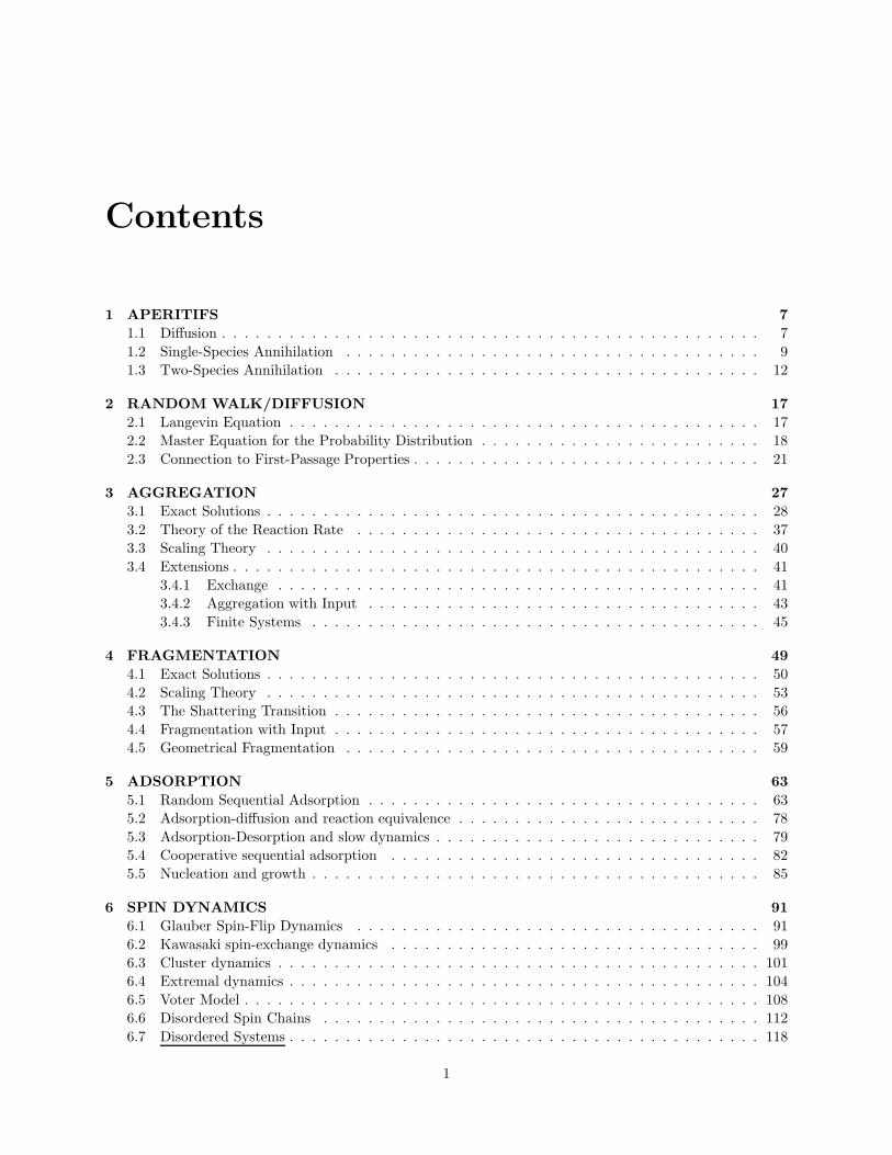
Figure 2.1: Diagrammatic relation between the occupation probability of a random walk (propagation isrepresented by a wavy line) and the first-passage probability (straight line).
We now present a simple-minded approach to understand this transition between recurrence and tran-sience. Let P (~r, t) be probability that a random walk is at ~r at time t when it starts at the origin. Similarly,

20 CHAPTER 2. RANDOM WALK/DIFFUSION
let F (~r, t) be the first-passage probability, namely, the probability that the random walk visits ~r for the first
time at time t with the same initial condition.
For a random walk to be at ~r at time t, the walk must first reach ~r at some earlier time step t′ and thenreturn to ~r after t− t′ (Fig. 2.1). This connection between F (~r, t) and P (~r, t) may therefore be expressed asthe convolution
P (~r, t) = δ~r,0δt,0 +
∫ t
0
F (~r, t′) P (0, t − t′) dt′. (2.3.1)
The delta function term accounts for the initial condition. The second term accounts for the ways that awalk can be at ~r at time t. To reach r at time t, the walk must first reach r at some time t,≤ t. Oncea first passage has occurred, the walk must return to r exactly at time t (and the walk can also return tor at earlier times, so long as the walk is also at r at time t). Because of the possibility of multiple visitsto ~r between time t′ and t, the return factor involves P rather than F . This convolution equation is mostconveniently solved in terms of the Laplace transform to give P (~r, s) = δ~r,0 +F (~r, s)P (0, s). Thus we obtainthe fundamental connection
F (~r, s) =
P (~r, s)
P (0, s), ~r 6= 0
1 − 1
P (0, s), ~r = 0,
(2.3.2)
in which the Laplace transform of the first-passage probability is determined by the corresponding transformof the probability distribution of diffusion P (~r, t).
We now use the techniques of Section A.2 to determine the time dependence of the first-passage probabilityin terms of the Laplace transform for the occupation probability. For isotropic diffusion, P (~r = 0, t) =(4πDt)−d/2 in d dimensions and the Laplace transform is P (0, s) =
∫ ∞0 P (0, t) e−st, dt. As discussed in
Section A.2, this integral has two fundamentally different behaviors, depending on whether∫ ∞
P (0, t) dtdiverges or converges. In the former case, we apply the last step in Eq. (A.2.1) to obtain
P (0, s) ∝∫ t∗=1/s
(4πDt)−d/2 dt ∼{
Ad(t∗)1−d/2 = Ads
d/2−1, d < 2
A2 ln t∗ = −A2 ln s, d = 2,(2.3.3)
where the dimension-dependent prefactor Ad is of the order of 1 and does not play any role in the asymptoticbehavior.
For d > 2, the integral∫ ∞
P (0, t) dt converges and one has to be more careful to extract the asymptoticbehavior by studying P (0, 1) − P (0, s). By such an approach, it is possible to show that P (0, s) has theasymptotic behavior
P (0, s) ∼ (1 −R)−1 + Bdsd/2−1 + . . . , d > 2, (2.3.4)
where R is the eventual return probability, namely, the probability that a diffusing particle random walkultimately reaches the origin, and Bd is another dimension-dependent constant of the order of 1. Using theseresults in Eq. (2.3.2), we infer that the Laplace transform for the first-passage probability has the asymptoticbehaviors
F (0, s) ∼
1 − Ads1−d/2, d < 2
1 + A2(ln s)−1, d = 2
R + Bd(1 −R)2sd/2−1, d > 2,
(2.3.5)
From this Laplace transform, we determine the time dependence of the survival probability by approxi-mation (A.2.7); that is,
F (0, s = 1 − 1/t∗) ∼∫ t∗
0
F (0, t) dt ≡ T (t∗), (2.3.6)
where T (t) is the probability that the particle gets trapped (reaches the origin) by time t and S(t) is thesurvival probability, namely, the probability that the particle has not reached the origin by time t. Herethe trick of replacing an exponential cutoff by a sharp cutoff provides an extremely easy way to invert the

2.3. CONNECTION TO FIRST-PASSAGE PROPERTIES 21
Laplace transform. From Eqs. (2.3.5) and (2.3.6) we thus find
S(t) ∼
Adt1−d/2, d < 2
A2(ln t)−1, d = 2
(1 −R) + Cd(1 −R)2t1−d/2, d > 2.
(2.3.7)
where Cd is another d-dependent constant of the order of 1. Finally, the time dependence of the first-passageprobability may be obtained from the basic relation 1 − S(t) ∼
∫ tF (0, t) dt to give
F (0, t) = −∂S(t)
∂t∝
td/2−2, d < 2
t−1(ln t)−2, d = 2
t−d/2, d > 2.
(2.3.8)
A crucial feature is that the asymptotic time dependence is determined by only by the spatial dimension.For d ≤ 2, the survival probability S(t) ultimately decays to zero. Thus a random walk is recurrent and iscertain to eventually return to its starting point, and indeed visit any site of an infinite lattice.
Finally, we outline a useful technique to compute where on a boundary is a diffusing particle absorbedand when does this absorption occur. This method will provide helpful in understanding finite-size effect inreaction kinetics. For simplicity, consider a symmetric nearest-neighbor random walk in the finite interval[0, 1]. Let E+(x) be the probability that a particle, which starts at x, eventually hits x = 1 without hittingx = 0. This eventual hitting probability E+(x) is obtained by summing the probabilities for all paths thatstart at x and reach 1 without touching 0. Thus
E+(x) =∑
p
Pp(x), (2.3.9)
where Pp(x) denotes the probability of a path from x to 1 that does not touch 0. The sum over all suchpaths can be decomposed into the outcome after one step (the factors of 1/2 below) and the sum over allpath remainders from the location after one step to 1. This gives
E+(x) =∑
p
[
1
2Pp(x + δx) +
1
2Pp(x − δx)
]
=1
2[E+(x + δx) + E+(x − δx)]. (2.3.10)
By a simple rearrangement, this equation is equivalent to
∆(2)E+(x) = 0, (2.3.11)
where ∆(2) is the second-difference operator. Notice the opposite sense of this recursion formula compared tothe master equation Eq. (2.2.1) for the probability distribution. Here E+(x) is expressed in terms of output
from x, while in the master equation, the occupation probability at x is expressed in terms of input to x. Forthis reason, Eq. (2.3.10) is sometimes referred to as a backward master equation. This backward equationis just the Laplace equation and gives a hint of the deep relation between first-passage properties, such asthe exit probability, and electrostatics. Equation (2.3.11) is subject to the boundary conditions E+(0) = 0and E+(1) = 1; namely if the walk starts at 1 it surely exits at 1 and if the walk starts at 0 it has nochance to exit at 1. In the continuum limit, Eq. (2.3.11) becomes the Laplace equation E ′′ = 0, subject toappropriate boundary conditions. We can now transcribe well-known results from electrostatics to solve theexit probability. For the one dimensional interval, the result is remarkably simple: E+(x) = x!
This exit probability also represents the solution to the classic “gambler’s ruin” problem: let x representyour wealth that changes by a small amount dx with equal probability in a single bet with a Casino. Youcontinue to bet as long as you have money. You lose if your wealth hits zero, while you break the Casinoif your wealth reaches 1. The exit probability to x = 1 is the same as the probability that you break theCasino.
Let’s now determine the mean time for a random walk to exit a domain. We focus on the unconditional
exit time, namely, the time for a particle to reach any point on the absorbing boundary of this domain. Forthe symmetric random walk, let the time increment between successive steps be δt, and let t(x) denote the

22 CHAPTER 2. RANDOM WALK/DIFFUSION
average exit time from the interval [0, 1] when a particle starts at x. The exit time is simply the time foreach exit path times the probability of the path, averaged over all trajectories, and leads to the analog ofEq. (2.3.9)
t(x) =∑
p
Pp(x) tp(x), (2.3.12)
where tp(x) is the exit time of a specific path to the boundary that starts at x.In analogy with Eq. (2.3.10), this mean exit time obeys the recursion
t(x) =1
2[(t(x + δx) + δt) + (t(x − δx) + δt)] , (2.3.13)
This recursion expresses the mean exit time starting at x in terms of the outcome one step in the future, forwhich the initial walk can be viewed as restarting at either x+δx or x−δx, each with probability 1/2, but alsowith the time incremented by δt. This equation is subject to the boundary conditions t(0) = t(1) = 0; theexit time equals zero if the particle starts at the boundary. In the continuum limit, this recursion formulareduces to the Poisson equation Dt′′(x) = −1. For diffusion in a d-dimensional domain with absorptionon a boundary B, the corresponding Poisson equation for the exit time is D∇2t(~r) = −1, subject to theboundary condition t(~r) = 0 for ~r ∈ B. Thus the determination of the mean exit time has been recast asa time-independent electrostatic problem! For the example of the unit interval, the solution to the Laplaceequation is just a second-order polynomial in x. Imposing the boundary conditions immediately leads to theclassic result
t(x) =1
2Dx(1 − x). (2.3.14)
Problems
1. Find the generating function for the Fibonacci sequence, Fn = Fn−1 + Fn−2, with the initial conditionF0 = F1 = 1; that is, determine F (z) =
∑∞0 Fnzn. Invert the generating function to find a closed form
expression for Fn.
2. Consider a random walk in one dimension in which a step to the right of length 2 occurs with probability1/3 and a step to the left of length 1 occurs with probability 2/3. Investigate the corrections to theisotropic Gaussian that characterizes the probability distribution in the long-time limit. Hint: Considerthe behavior of moments beyond second order, 〈xk〉 with k > 2.
3. Solve the gambler’s ruin problem when the probability of winning in a single bet is p. The bettinggame is repeated until either you are broke or the casino is broken. Take the total amount of capital tobe $N and you start with $n. What is the probability that you will break the casino? Also determinethe mean time until the betting is over (either you are broke or the Casino is broken). More advanced:
Determine the mean time until betting is over with the condition that: (i) you are broke, and (ii) youbreak the Casino. Solve this problem both for fair betting and biased betting.
4. Consider the gambler’s ruin problem under the assumptions that you win each bet with probabilityp 6= 1/2, but that the casino has an infinite reserve of money. What is the probability that you breakthe casino as a function of p? For those values of p where you break the casino, what is the averagetime for this event to occur?
Notes
The field of random walks, diffusion, and first-passage processes are classic areas of applied probabilitytheory and there is a corresponding large literature. For the more probabilistic aspects of random walks andprobability theory in general, we recommend 8; 3; 2; 9. For the theory of random walks and diffusion froma physicist’s perspective, we recommend W,RG,MW. For first-passage properties, please consult 8; 9.

Bibliography
W. Feller, An Introduction to Probability Theory and its Applications, Vol 1, (Wiley, New York, 1968).
S. Karlin and H. M. Taylor, A First Course in Stochastic Processes 2nd ed. (Academic Press, New York,1975).
G. H. Weiss, Aspects and Applications of the Random Walk (North-Holland, Amsterdam, 1994).
J. Rudnick, G. Gaspari, Elements of the Random Walk, (Cambridge University Press, New York, 2004).
E. Montroll, Random walks on lattices in Proceedings of the Symposiusm on Applied Mathematics (AmericanMathematical Society, Providence, RI), Vol. 16, pp. 193–230 (1965); E. Montroll and G. H. Weiss, Random
walks on lattices. II., J. Math. Phys. 6, 167–181 (1965).
S. Redner, A Guide to First-Passage Processes (Cambridge University Press, Cambridge, 2001).
N. G. Van Kampen, Stochastic Processes in Physics and Chemistry, 3rd edition (North-Holland, Amster-dam, 2001).
S. Chandrasekhar, Rev. Mod. Phys. 15, 1 (1943).
23

24 BIBLIOGRAPHY

Chapter 3
AGGREGATION
Aggregation is a fundamental non-equilibrium process in which reactive clusters join together irreversiblywhen they meet (Fig. 3.1) so that the typical mass of a collection of aggregates grows monotonically withtime. Developing an understanding aggregation is important both because of its ubiquitous applications—such as the gelation of jello, the curdling of milk, the coagulation of blood, and the formation of stars bygravitational accretion—and because aggregation is an ideal setting to illustrate theoretical analysis tools.We schematically write aggregation as
Ai + AjKij−→Ai+j .
That is, a cluster of mass i + j is created at an intrinsic rate Kij by the aggregation of a cluster of mass iand a cluster of mass j. The fundamental observables of the system are ck(t), the concentration of clustersof mass k at time t.
j
i+ji
Figure 3.1: Schematic representation of aggregation. A cluster of mass i and mass j react to create a clusterof mass i + j.
The primary goal of this chapter is to elucidate the basic features of the mass distribution ck(t) andto understand which features of the reaction rate Kij influence this distribution. In pursuit of this goal,we will write the master equations that describe the evolution of the cluster mass distribution in an infinitesystem and discuss some of its elementary properties. Next, we work out exact solutions for specific examplesto illustrate both the wide range of phenomenology and the many useful techniques for analyzing masterequations. We will then discuss the reaction rate in general terms and show how to calculate this rate. Thisdiscussion will naturally lead to the notion of dynamical scaling, which provides a simple way to obtain ageneral understanding of aggregation. Finally, we will discuss several important extensions of aggregationthat exhibit rich kinetic properties.
The Master Equations
The traditional starting point for treating aggregation is the infinite set of equations that describe how thecluster mass distribution changes with time. For a general reaction rate Kij , the master equations are:
ck(t) =1
2
∑
i,ji+j=k
Kij ci(t) cj(t) − ck(t)∞∑
i=1
Kik ci(t). (3.0.1)
25