CONTENTSAlgebra

Chapter 1 Exponents and logarithms1.1 Laws of exponents 21.2 Conversion between exponents and logarithms 61.3 Logarithm laws 81.4 Exponential and logarithmic equations 10

Chapter 2 Sequences and series2.1 Arithmetic sequences and series 172.2 Geometric sequences and series 222.3 Sigma notation 28

Chapter 3 The binomial theorem3.1 Pascal’s triangle 323.2 Binomial theorem 32

Functions and equations

Chapter 4 Introduction to functions4.1 Finding function values 404.2 Domain and range 414.3 Composite functions 434.4 Inverse functions 46

Chapter 5 Graphs of functions5.1 Quadratic functions and their graphs 525.2 Reciprocal functions and rational functions 655.3 Graphs of inverse functions 685.4 Transformations of graphs 72

Chapter 6 Exponential and logarithmic functions6.1 Exponential and logarithmic functions 856.2 Applications 93

Circular functions and trigonometry

Chapter 7 Radian angle measure and sectors7.1 Definition of a radian 1007.2 Length of an arc and area of a sector 102

Chapter 8 Trigonometric functions8.1 Sine, cosine, and tangent functions 1108.2 Trigonometric identities 1238.3 Graphs of trigonometric functions 1288.4 Applications 1378.5 Trigonometric equations 144

Chapter 9 Trigonometry of non-right angled triangles9.1 The cosine rule 1539.2 The sine rule 1569.3 Area of a triangle 1609.4 Applications to geometric problems 165

Vectors

Chapter 10 Vector algebra10.1 Basic vector concepts 17410.2 Algebraic operations of vectors in component form 17810.3 Scalar products 192

Chapter 11 Vector equations of lines11.1 Vector equation of a line 20311.2 Angle between two lines 20911.3 Relationships between two lines 214

Calculus

Chapter 12 Differential calculus12.1 Derivatives of functions 22412.2 Differentiation rules 22912.3 Higher order derivatives 237

Chapter 13 Applications of differentiation13.1 Tangents and normals 24113.2 Increasing and decreasing functions 24713.3 Local maximums and minimums of functions 25113.4 Concavity of functions 25413.5 Graphical behaviour of functions 26113.6 Optimization 27013.7 Kinematics 274

Chapter 14 Integral calculus14.1 Indefinite integrals 28114.2 Integration by inspection and substitution 28714.3 Definite integrals 292

Chapter 15 Applications of integration15.1 Areas under curves 29815.2 Volumes of revolution 31215.3 Kinematics and combined integration problems 319

Statistics and probability

Chapter 16 Statistics measures16.1 Basic concepts 33016.2 Measures of central tendency for ungrouped data 33116.3 Measures of central tendency for grouped data 33216.4 Quartiles and percentiles 33316.5 Measures of dispersion 33416.6 Transformations on data sets 33616.7 Frequency curves and histograms 34016.8 Box and whisker plots 348

Chapter 17 Bivariate statistics17.1 Linear correlation of bivariate data 35917.2 Use of the equation of the regression line for prediction purposes 364

Chapter 18 Probability18.1 Introduction to probability 36818.2 Combined events 36918.3 Venn diagrams and tree diagrams 37118.4 Conditional probability and independent events 379

Chapter 19 Probability distributions19.1 Discrete random variables 39219.2 Binomial probability distribution 39819.3 Normal distribution 403

Mathematical symbols and notation 415

Practice test 1

Practice test 2

Answers and markschemes can be downloaded for free at www.ntk.edu.hk.

In Paper 1 of the IB SL exam, you are expected to know the properties of the graphs of some basic functions. In Paper 2, you may also need to use a graphic display calculator (GDC) to analyse the graphs of more complicated functions.

Basic terminology:

y-intercept: The intersection of the graph of ( )f x and the y-axis

x-intercept: The intersection of the graph of ( )f x and the x-axis

Asymptote: A straight line whose distance to the graph of ( )f x tends to zero (that is, the graph of ( )f x gets closer and closer to the asymptote.)

O x

yy-intercept

x-intercept

asymptote EXAM TIP

The x-intercept and y-intercept can usually be found by a GDC in Paper 2.

5.1 Quadratic functions and their graphs

General form

The general expression of a quadratic function is ( ) = + +f x ax bx c2 , where a ≠ 0. Its graph is in the shape of a parabola. The orientation of the parabola is determined by the sign of the coefficient a of the x2 term. The lowest or highest point on the parabola is called the vertex (plural: “vertices”).

If a > 0, the parabola opens upward. If a < 0, the parabola opens downward.

e.g. ( ) = +f x x x22 e.g. ( ) = + +−f x x x2 102

O x

y

vertexO x

yvertex

Graphs of functions5C h a p t e r

52 Functions and equations

From the graphs above, you can see that the graph of a quadratic function is symmetric about a vertical straight line through the vertex. The equation of the line is given by:

This is given in your formula booklet

= −x ba2

This vertical line is called the axis of symmetry.

Vertex form

By completing the square, we can rewrite the quadratic function ( ) = + +f x ax bx c2 in vertex form.

If ( ) = + +f x ax bx c2 , then ( )f x can be written as (( )) (( ))== −− ++f x a x h k2

, where

( )h k, are the coordinates of the vertex of the graph of f.

O x

y

h,k( )

Find the coordinates of the vertex of the graph of a y = x2 + 6x − 1b y = x2 − 3x + 5

a

y x x

x

x

6 1

3 9 1

3 10

2

2

2

( )

( )

= + −

= + − −

= + −

Vertex is at 3, 10( )− − .

Solution

Example 5-1

Divide the x-coefficient by 2

Copy the constant term

Square the 3 and subtract

EXAM TIPCompleting the square is an essential skill for the IBDP SL exam. Candidates are expected to be able to change quadratic functions from one form to another.

53Chapter 5 Graphs of functions

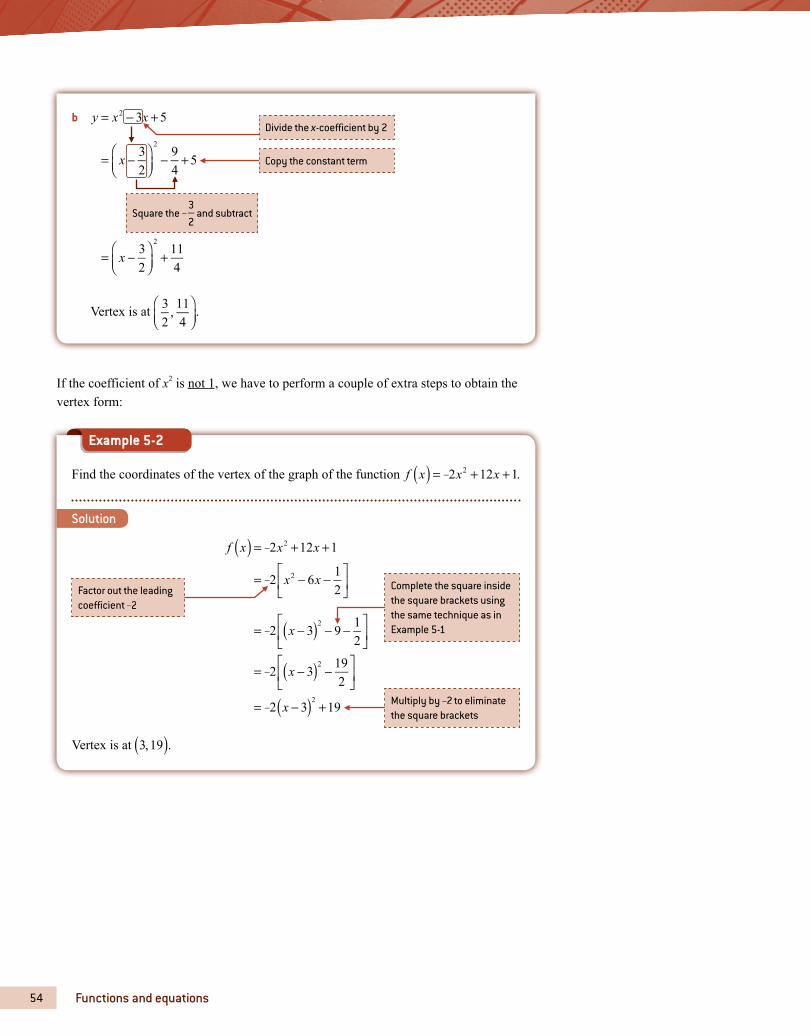
b

y = x2 3x + 5

= x 32

294

+ 5

= x 32

2

+ 114

Vertex is at 32

, 114

.

Divide the x-coefficient by 2

Copy the constant term

Square the 32

− and subtract

If the coefficient of x2 is not 1, we have to perform a couple of extra steps to obtain the vertex form:

Find the coordinates of the vertex of the graph of the function f x x x2 12 12( ) = + +− .

f x( ) = 2x2 +12x +1

= 2 x2 6x 12

= 2 x 3( )29 1

2

= 2 x 3( )2 192

= 2 x 3( )2+19

Vertex is at 3,19( ).

Solution

Example 5-2

Factor out the leading coefficient 2−

Multiply by 2− to eliminate the square brackets

Complete the square inside the square brackets using the same technique as in Example 5-1

54 Functions and equations

The expression under the radical sign b2 − 4ac is called the discriminant and is usually denoted by Δ. Its value enables us to find the number of real solutions to the corresponding quadratic equation.

Discriminant Number of real solutions Typical graph

Δ = b2 − 4ac > 0Two distinct real solutions

(two x-intercepts)

O x

y

Δ = b2 − 4ac = 0

One real solution(one x-intercept)

(This is also called a repeated root)

O x

y

Δ = b2 − 4ac < 0No real solutions(no x-intercepts)

O x

y

How many real solutions do the following equations have?a x2 + x + 2 = 0b − + =−x x2 5 02

c 4x2 + 8x + 4 = 0

a a = 1, b = 1, c = 2

Hence

= b2 4ac= 12 4 1( ) 2( )= 7< 0

∴ no real solutions

Solution

Example 5-8

You don’t have to write down the values of a, b and c, but writing them can help minimize mistakes, especially with more complicated situations.

COMMON MISTAKEDon’t confuse the discriminant and the quadratic formula. The discriminant only tells you how many solutions there are; the quadratic formula gives the actual values.

59Chapter 5 Graphs of functions

Step 3 – A vertical stretch by a scale factor of 13: ( )= −y x1

32 4

2

1 2 3

8

5 6 7

2

4

6

4Ox

y

123

Step 4 – A vertical translation of 2 units upward: ( )= − +y x132 4 2

2

1 2 3

8

5 6 7123

2

4

6

4Ox

y

Warm-up Exercise 5D

1 The graph of ( )=y f x is shown below.

O x

y

2−1−

y = f x( )

Sketch the graph of each of the following:

a ( )= +y f x 3 b ( )= +y f x 3

c y f x( )= − d y f x 3( )= −

e ( )=y f x2 f ( )=y f x2

( )−x2 4 2 is multiplied by 13

to

get ( )−x13

2 4 2. This is a vertical

stretch by a factor of 13

.

2 is added to the whole

expression ( )−x13

2 4 2. This is a

vertical shift up 2 units.

77Chapter 5 Graphs of functions

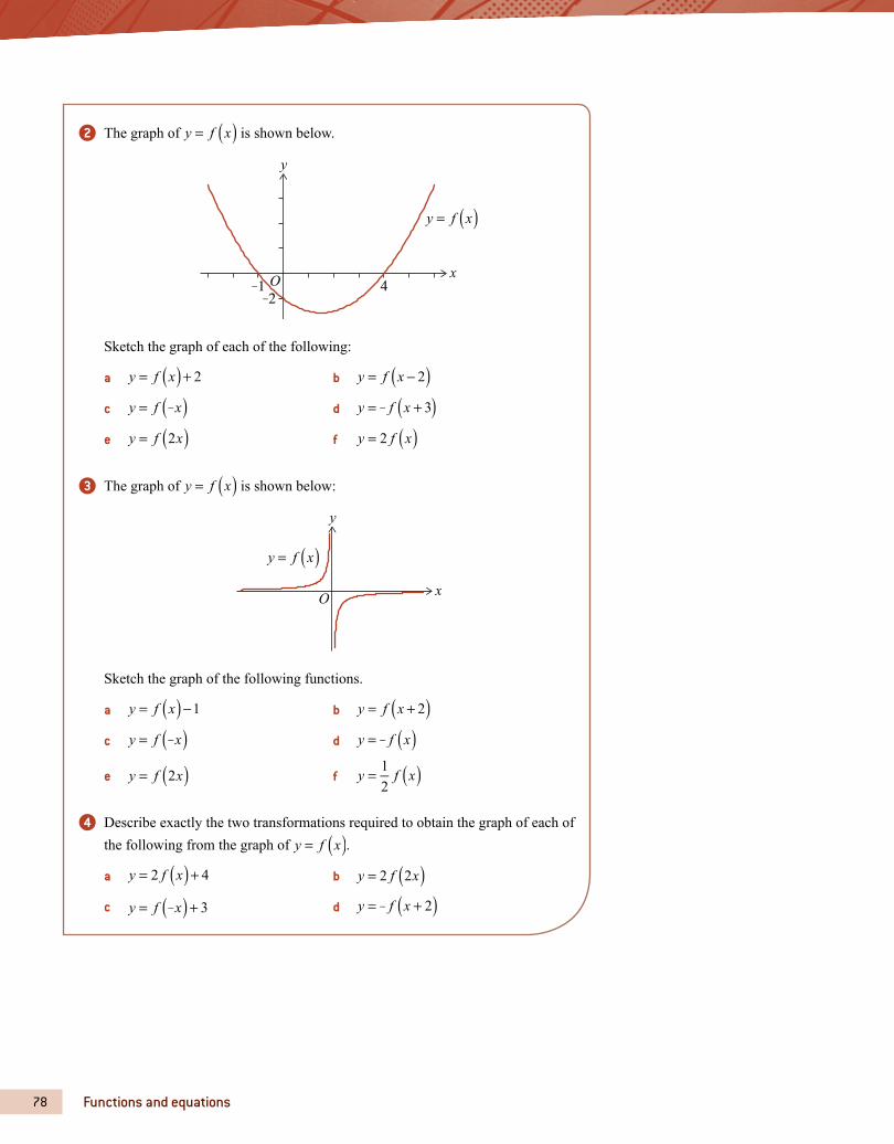
2 The graph of y f x( )= is shown below.

4O x

y

1−2−

y = f x( )

Sketch the graph of each of the following:

a ( )= +y f x 2 b ( )= −y f x 2

c y f x( )= − d y f x 3( )= +−

e ( )=y f x2 f ( )=y f x2

3 The graph of y f x( )= is shown below:

O x

y

y = f x( )

Sketch the graph of the following functions.

a ( )= −y f x 1 b ( )= +y f x 2

c y f x( )= − d y f x( )= −

e ( )=y f x2 f ( )=y f x12

4 Describe exactly the two transformations required to obtain the graph of each of the following from the graph of y f x( )= .

a ( )= +y f x2 4 b ( )=y f x2 2

c y f x 3( )= +− d y f x 2( )= +−

78 Functions and equations

5 Express the function ( )g x in terms of ( )f x where the graph of ( )=y g x can be

obtained by applying the following transformations to the graph of ( )=y f x .

a Translate by the vector 23

.

b Move downward 2 units and then move to the right by 3 units.

c Move to the left 3 units and then stretch vertically by a factor of 12

.

d Reflect about the x-axis and then stretch horizontally by a factor of 15

.

e Stretch horizontally by a factor of 3 and then stretch vertically by a factor of 13.

f Reflect about the y-axis and then move downward by 2 units.g Move upward by 7 units and then reflect about the x-axis.

Exam Practice 5D

Paper 1

1 The graph of ( )=y f x , x3 3≤ ≤− , is shown below. Sketch the graph of

( )= − +y f x 1 2 on the same axes.

O x

y5

33 1

y = f x( )

2 The graph of ( )=y f x is transformed into the graph of ( )= − +y f x5 3 1. Give a full geometric description of this transformation.

79Chapter 5 Graphs of functions

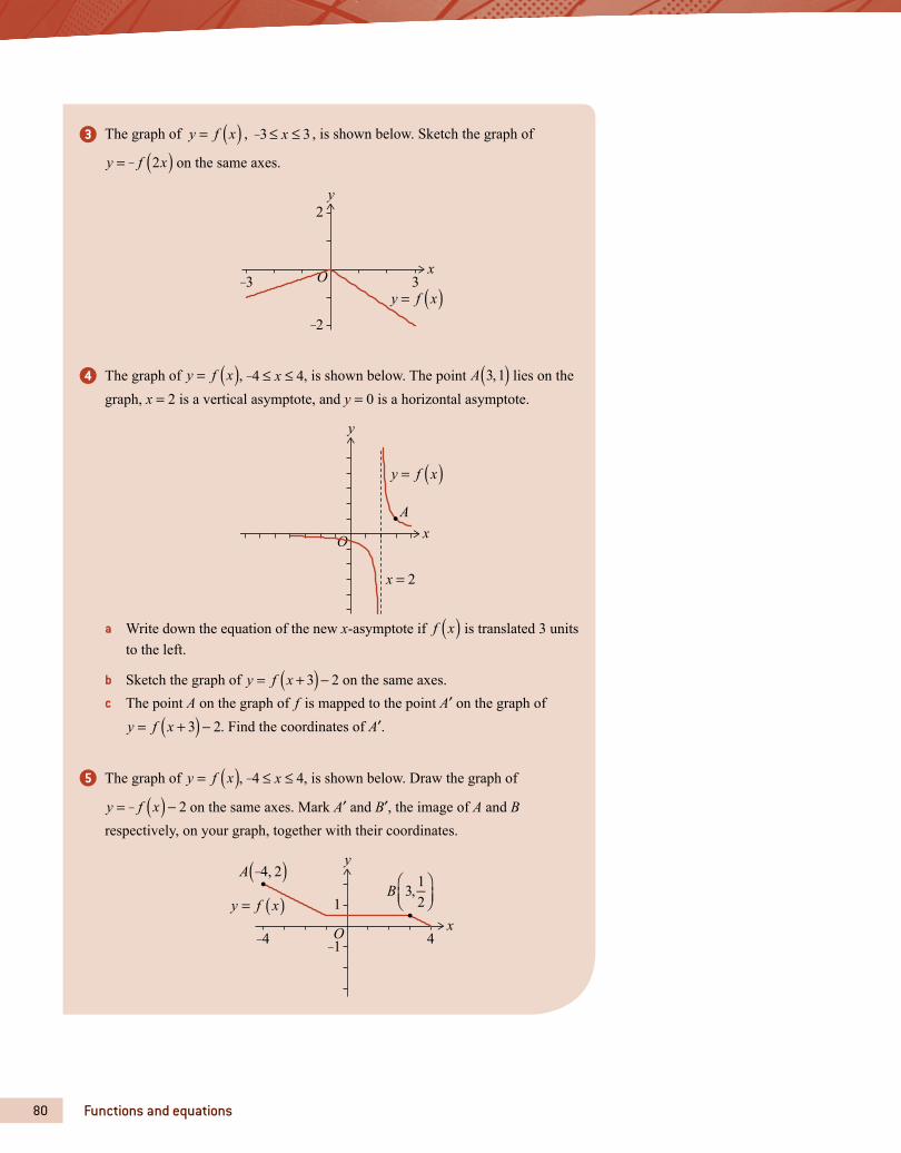
3 The graph of ( )=y f x , x3 3≤ ≤− , is shown below. Sketch the graph of

y f x2( )= − on the same axes.

O x

y2

33

2

y = f x( )

4 The graph of ( )=y f x , x4 4≤ ≤− , is shown below. The point ( )A 3,1 lies on the graph, x = 2 is a vertical asymptote, and y = 0 is a horizontal asymptote.

O x

A

y

x = 2

y = f x( )

a Write down the equation of the new x-asymptote if f x( ) is translated 3 units to the left.

b Sketch the graph of ( )= + −y f x 3 2 on the same axes.c The point A on the graph of f is mapped to the point A′ on the graph of y f x 3 2( )= + − . Find the coordinates of A′.

5 The graph of ( )=y f x , x4 4≤ ≤− , is shown below. Draw the graph of

y f x 2( )= −− on the same axes. Mark A′ and B′, the image of A and B respectively, on your graph, together with their coordinates.

O x

y

y f x= ( ) 1

414

A 4, 2( )B 3, 1

2

80 Functions and equations

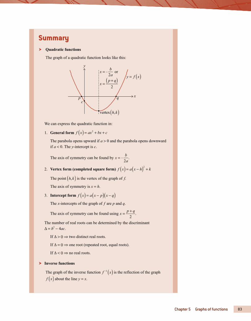
Summary Quadratic functions

The graph of a quadratic function looks like this:

x

y

y = f x( )

vertex h,k( )

qpc

x = b2a

or

x =p + q( )

2

We can express the quadratic function in:

1. General form ( ) = + +f x ax bx c2

The parabola opens upward if a > 0 and the parabola opens downward if a < 0. The y-intercept is c.

The axis of symmetry can be found by x ba2

= − .

2. Vertex form (completed square form) ( ) ( )= − +f x a x h k2

The point ( )h k, is the vertex of the graph of f.

The axis of symmetry is x = h.

3. Intercept form ( ) ( )( )= − −f x a x p x q

The x-intercepts of the graph of f are p and q.

The axis of symmetry can be found using =+x p q2

.

The number of real roots can be determined by the discriminant Δ = b2 − 4ac.

If Δ > 0 ⇒ two distinct real roots.

If Δ = 0 ⇒ one root (repeated root, equal roots).

If Δ < 0 ⇒ no real roots.

Inverse functions

The graph of the inverse function ( )−f x1 is the reflection of the graph

( )f x about the line y = x.

83Chapter 5 Graphs of functions