Content analysis for audio classification and segmentation - Speech · PDF file · 2017-03-22segmenting an audio stream into speech, music, environment sound, ... works on audio content

504 IEEE TRANSACTIONS ON SPEECH AND AUDIO PROCESSING, VOL. 10, NO. 7, OCTOBER 2002

Content Analysis for Audio Classification andSegmentation

Lie Lu, Hong-Jiang Zhang, Senior Member, IEEE, and Hao Jiang

Abstract—In this paper, we present our study of audio contentanalysis for classification and segmentation, in which an audiostream is segmented according to audio type or speaker identity.We propose a robust approach that is capable of classifying andsegmenting an audio stream into speech, music, environmentsound, and silence. Audio classification is processed in two steps,which makes it suitable for different applications. The first step ofthe classification is speech and nonspeech discrimination. In thisstep, a novel algorithm based on K-nearest-neighbor (KNN) andlinear spectral pairs-vector quantization (LSP-VQ) is developed.The second step further divides nonspeech class into music,environment sounds, and silence with a rule-based classificationscheme. A set of new features such as the noise frame ratio andband periodicity are introduced and discussed in detail. Wealso develop an unsupervised speaker segmentation algorithmusing a novel scheme based on quasi-GMM and LSP correlationanalysis. Without a priori knowledge, this algorithm can supportthe open-set speaker, online speaker modeling and real timesegmentation. Experimental results indicate that the proposedalgorithms can produce very satisfactory results.

Index Terms—Audio classification and segmentation, audio con-tent analysis, speaker change detection, speaker segmentation.

I. INTRODUCTION

A UDIO classification and segmentation can provide usefulinformation for both audio content understanding and

video content analysis. Therefore, in addition to the classicalworks on audio content analysis for audio classification andaudio retrieval [1], [2], recent works have also integrated audioand visual information [12]–[14] in video structure parsing andcontent analysis. In general, the application of audio contentanalysis in video parsing can be considered in two parts. Oneis to classify or segment an audio stream into different soundclasses such as speech, music, environment sound, and silence;the other is to classify speech streams into segments of differentspeakers. In this paper, our research works on these two taskswill be presented.

Intensive studies have been conducted on audio classificationand segmentation by employing different features and methods.In spite of these research efforts, high-accuracy audio classifica-tion is only achieved for simple cases such as speech/music dis-crimination. Pfeifferet al.[3] presented a theoretical framework

Manuscript received December 5, 2001; revised July 11, 2002. The associateeditor coordinating the review of this manuscript and approving it for publica-tion was Prof. C.-C. Jay Kuo.

L. Lu and H.-J. Zhang are with Microsoft Research Asia, Beijing 100080,China (e-mail: [email protected]; [email protected]).

H. Jiang was with Microsoft Research Asia, Beijing 100080, China. He isnow with Simon Fraser University, Vancouver, BC V6B 5K3, Canada (e-mail:[email protected]).

Digital Object Identifier 10.1109/TSA.2002.804546

and application of automatic audio content analysis using someperceptual features. Saunders [4] presented a speech/music clas-sifier based on simple features such as zero-crossing rate andshort-time energy for radio broadcast. The paper reported thatthe accuracy rate can achieve 98% when a window size of 2.4s is used. Meanwhile, Scheireret al. [5] introduced more fea-tures for audio classification and performed experiments withdifferent classification models including GMM, BP-ANN, andKNN. When using a window of the same size (2.4 s), the re-ported error rate is 1.4%. However, it is found that these simplefeatures-based methods cannot offer satisfactory results particu-larly when a smaller window is used or when more audio classessuch as environment sounds are taken into consideration.

Many other works have been conducted to enhance audioclassification algorithms. In [6], audio recordings are classifiedinto speech, silence, laughter, and nonspeech sounds, to segmentdiscussion recordings in meetings. In the work by Zhang andKuo [7], pitch tracking methods were introduced to discriminateaudio recordings into classes such as songs and speeches overmusic, based on a heuristic-based model. Accuracy of greaterthan 90% was reported. Srinivasan [12] proposed an approachto detect and classify audio that consists of mixed classes suchas combinations of speech and music together with environmentsound. The accuracy of classification is more than 80%.

In this paper, we present a high-accuracy algorithm for audioclassification and segmentation. Speech, music, environmentsound, and silence, the basic sets required in audio/videocontent analysis, are discriminated in a 1-s window, which isshorter than the testing unit used in [4] and [5]. Compared toother methods, our algorithm is computationally inexpensiveand more practical for different applications. In order toimprove the classification of the four audio classes in term ofaccuracy and robustness, a set of new features includingbandperiodicity is proposed and discussed in detail.

Another novel work contributed in this paper is the real-timeunsupervised speaker segmentation. We segment a speechsequence into segments of different speakers. Unlike generalspeaker identification or verification, no prior knowledge aboutthe number and identities of speakers in an audio clip areassumed. In video browsing, if a speaker is first registered, atraditional speaker identification algorithm can be used, just asin the work of Brummer [16]. In video parsing applications,the knowledge of speakers is often not available or difficultto acquire. Therefore, it is desirable to perform unsupervisedspeaker segmentation in audio analysis.

There are several reported works on unsupervised speakeridentification and clustering. Sugiyama [17] studied a simplercase, in which the number of the speakers to be clustered was

1063-6676/02$17.00 © 2002 IEEE

LU et al.: CONTENT ANALYSIS FOR AUDIO CLASSIFICATION AND SEGMENTATION 505

assumed known. Wilcox [18], in contrast, proposed an algo-rithm based on HMM segmentation, where an agglomerativeclustering method is used when the prior knowledge of speakersis unknown. Another system [19], [20] was proposed to sepa-rate controller speech and pilot speech with the GMM model,in addition to the speech and noise detection that were also con-sidered in the framework. Speaker discrimination from the tele-phone speeches was studied in [21] using HMM segmentation.However, in this system, the number of speakers was limited totwo. Mori [22] addresses the problem of speaker changes detec-tion and speaker clustering withouta priori speaker informa-tion available. Chen [23] also presented an approach to detectchanges in speaker identity, environmental and channel condi-tions by using the Bayesian information criterion. An accuracyof 80% was reported.

Previous efforts to tackle the problem of unsupervisedspeaker clustering consist of clustering audio segments intohomogeneous clusters according to speaker identity, back-ground conditions, or channel conditions. Most methods usedcan be classified into two categories. One is based on VQ orclustering (GMM model), the other one is based on HMMmodel. A deficiency of these models is that they cannot meetthe real-time requirement, since a computationally intensiveiterative operation is utilized.

Real-time speaker segmentation is required in many applica-tions, such as speaker tracking in real-time news-video segmen-tation and classification, or real-time speaker adapted speechrecognition. In this paper, we present a real-time, yet effectiveand robust speaker segmentation algorithm based on LSP corre-lation analysis. Both the speaker identities and speaker numberare assumed unknown. The proposed incremental speaker up-dating and segmental clustering schemes ensure our method canbe processed in real-time with limited delay.

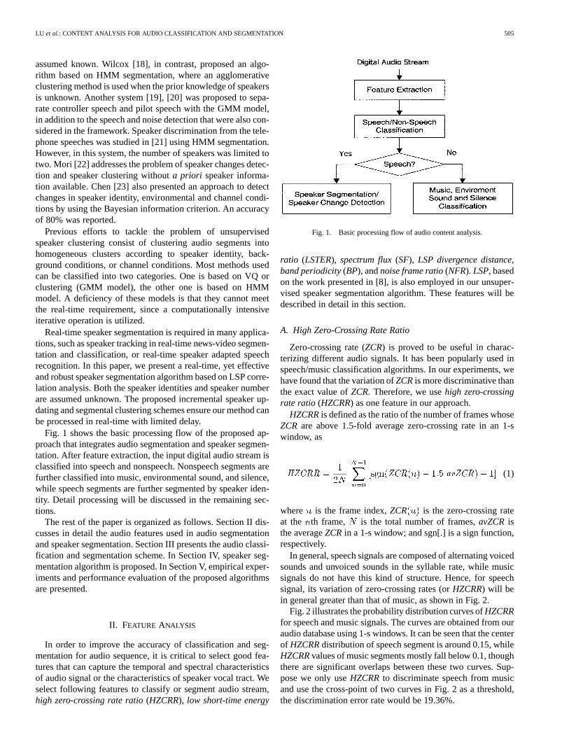
Fig. 1 shows the basic processing flow of the proposed ap-proach that integrates audio segmentation and speaker segmen-tation. After feature extraction, the input digital audio stream isclassified into speech and nonspeech. Nonspeech segments arefurther classified into music, environmental sound, and silence,while speech segments are further segmented by speaker iden-tity. Detail processing will be discussed in the remaining sec-tions.

The rest of the paper is organized as follows. Section II dis-cusses in detail the audio features used in audio segmentationand speaker segmentation. Section III presents the audio classi-fication and segmentation scheme. In Section IV, speaker seg-mentation algorithm is proposed. In Section V, empirical exper-iments and performance evaluation of the proposed algorithmsare presented.

II. FEATURE ANALYSIS

In order to improve the accuracy of classification and seg-mentation for audio sequence, it is critical to select good fea-tures that can capture the temporal and spectral characteristicsof audio signal or the characteristics of speaker vocal tract. Weselect following features to classify or segment audio stream,high zero-crossing rate ratio(HZCRR), low short-time energy

Fig. 1. Basic processing flow of audio content analysis.

ratio (LSTER), spectrum flux(SF), LSP divergence distance,band periodicity(BP), andnoise frame ratio(NFR). LSP, basedon the work presented in [8], is also employed in our unsuper-vised speaker segmentation algorithm. These features will bedescribed in detail in this section.

A. High Zero-Crossing Rate Ratio

Zero-crossing rate (ZCR) is proved to be useful in charac-terizing different audio signals. It has been popularly used inspeech/music classification algorithms. In our experiments, wehave found that the variation ofZCRis more discriminative thanthe exact value ofZCR. Therefore, we usehigh zero-crossingrate ratio (HZCRR) as one feature in our approach.

HZCRRis defined as the ratio of the number of frames whoseZCR are above 1.5-fold average zero-crossing rate in an 1-swindow, as

HZCRR ZCR avZCR (1)

where is the frame index,ZCR is the zero-crossing rateat the th frame, is the total number of frames,avZCRisthe averageZCRin a 1-s window; and sgn[.] is a sign function,respectively.

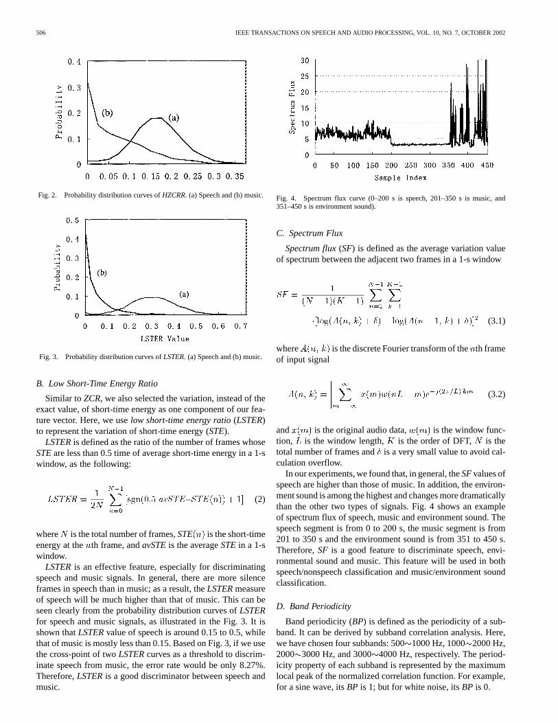
In general, speech signals are composed of alternating voicedsounds and unvoiced sounds in the syllable rate, while musicsignals do not have this kind of structure. Hence, for speechsignal, its variation of zero-crossing rates (orHZCRR) will bein general greater than that of music, as shown in Fig. 2.

Fig. 2 illustrates the probability distribution curves ofHZCRRfor speech and music signals. The curves are obtained from ouraudio database using 1-s windows. It can be seen that the centerof HZCRRdistribution of speech segment is around 0.15, whileHZCRRvalues of music segments mostly fall below 0.1, thoughthere are significant overlaps between these two curves. Sup-pose we only useHZCRRto discriminate speech from musicand use the cross-point of two curves in Fig. 2 as a threshold,the discrimination error rate would be 19.36%.


Fig. 2. Probability distribution curves ofHZCRR. (a) Speech and (b) music.

Fig. 3. Probability distribution curves ofLSTER. (a) Speech and (b) music.

B. Low Short-Time Energy Ratio

Similar toZCR, we also selected the variation, instead of theexact value, of short-time energy as one component of our fea-ture vector. Here, we uselow short-time energy ratio(LSTER)to represent the variation of short-time energy (STE).

LSTERis defined as the ratio of the number of frames whoseSTEare less than 0.5 time of average short-time energy in a 1-swindow, as the following:

LSTER avSTE–STE (2)

where is the total number of frames,STE is the short-timeenergy at the th frame, andavSTEis the averageSTEin a 1-swindow.

LSTERis an effective feature, especially for discriminatingspeech and music signals. In general, there are more silenceframes in speech than in music; as a result, theLSTERmeasureof speech will be much higher than that of music. This can beseen clearly from the probability distribution curves ofLSTERfor speech and music signals, as illustrated in the Fig. 3. It isshown thatLSTERvalue of speech is around 0.15 to 0.5, whilethat of music is mostly less than 0.15. Based on Fig. 3, if we usethe cross-point of twoLSTERcurves as a threshold to discrim-inate speech from music, the error rate would be only 8.27%.Therefore,LSTERis a good discriminator between speech andmusic.

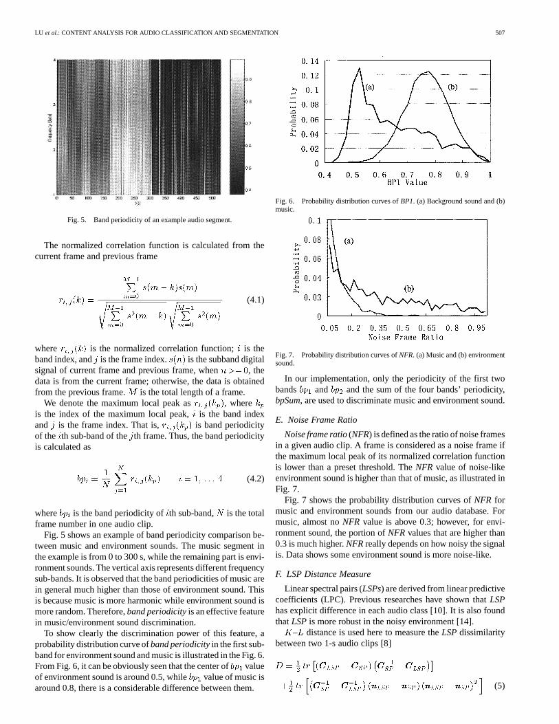
Fig. 4. Spectrum flux curve (0–200 s is speech, 201–350 s is music, and351–450 s is environment sound).

C. Spectrum Flux

Spectrum flux(SF) is defined as the average variation valueof spectrum between the adjacent two frames in a 1-s window

SF

(3.1)

where is the discrete Fourier transform of theth frameof input signal

(3.2)

and is the original audio data, is the window func-tion, is the window length, is the order of DFT, is thetotal number of frames andis a very small value to avoid cal-culation overflow.

In our experiments, we found that, in general, theSFvalues ofspeech are higher than those of music. In addition, the environ-ment sound is among the highest and changes more dramaticallythan the other two types of signals. Fig. 4 shows an exampleof spectrum flux of speech, music and environment sound. Thespeech segment is from 0 to 200 s, the music segment is from201 to 350 s and the environment sound is from 351 to 450 s.Therefore,SF is a good feature to discriminate speech, envi-ronmental sound and music. This feature will be used in bothspeech/nonspeech classification and music/environment soundclassification.

D. Band Periodicity

Band periodicity (BP) is defined as the periodicity of a sub-band. It can be derived by subband correlation analysis. Here,we have chosen four subbands: 5001000 Hz, 1000 2000 Hz,2000 3000 Hz, and 30004000 Hz, respectively. The period-icity property of each subband is represented by the maximumlocal peak of the normalized correlation function. For example,for a sine wave, itsBP is 1; but for white noise, itsBP is 0.


Fig. 5. Band periodicity of an example audio segment.

The normalized correlation function is calculated from thecurrent frame and previous frame

(4.1)

where is the normalized correlation function;is theband index, and is the frame index. is the subband digitalsignal of current frame and previous frame, when , thedata is from the current frame; otherwise, the data is obtainedfrom the previous frame. is the total length of a frame.

We denote the maximum local peak as , whereis the index of the maximum local peak,is the band indexand is the frame index. That is, is band periodicityof the th sub-band of theth frame. Thus, the band periodicityis calculated as

(4.2)

where is the band periodicity ofth sub-band, is the totalframe number in one audio clip.

Fig. 5 shows an example of band periodicity comparison be-tween music and environment sounds. The music segment inthe example is from 0 to 300 s, while the remaining part is envi-ronment sounds. The vertical axis represents different frequencysub-bands. It is observed that the band periodicities of music arein general much higher than those of environment sound. Thisis because music is more harmonic while environment sound ismore random. Therefore,band periodicityis an effective featurein music/environment sound discrimination.

To show clearly the discrimination power of this feature, aprobability distribution curve ofband periodicityin the first sub-band for environment sound and music is illustrated in the Fig. 6.From Fig. 6, it can be obviously seen that the center ofvalueof environment sound is around 0.5, while value of music isaround 0.8, there is a considerable difference between them.

Fig. 6. Probability distribution curves ofBP1. (a) Background sound and (b)music.

Fig. 7. Probability distribution curves ofNFR. (a) Music and (b) environmentsound.

In our implementation, only the periodicity of the first twobands and and the sum of the four bands’ periodicity,bpSum, are used to discriminate music and environment sound.

E. Noise Frame Ratio

Noise frame ratio(NFR) is defined as the ratio of noise framesin a given audio clip. A frame is considered as a noise frame ifthe maximum local peak of its normalized correlation functionis lower than a preset threshold. TheNFR value of noise-likeenvironment sound is higher than that of music, as illustrated inFig. 7.

Fig. 7 shows the probability distribution curves ofNFR formusic and environment sounds from our audio database. Formusic, almost noNFR value is above 0.3; however, for envi-ronment sound, the portion ofNFRvalues that are higher than0.3 is much higher.NFRreally depends on how noisy the signalis. Data shows some environment sound is more noise-like.

F. LSP Distance Measure

Linear spectral pairs (LSPs) are derived from linear predictivecoefficients (LPC). Previous researches have shown thatLSPhas explicit difference in each audio class [10]. It is also foundthatLSPis more robust in the noisy environment [14].

– distance is used here to measure theLSPdissimilaritybetween two 1-s audio clips [8]

LSP SP SP LSP

SP LSP LSP SP LSP SP (5)


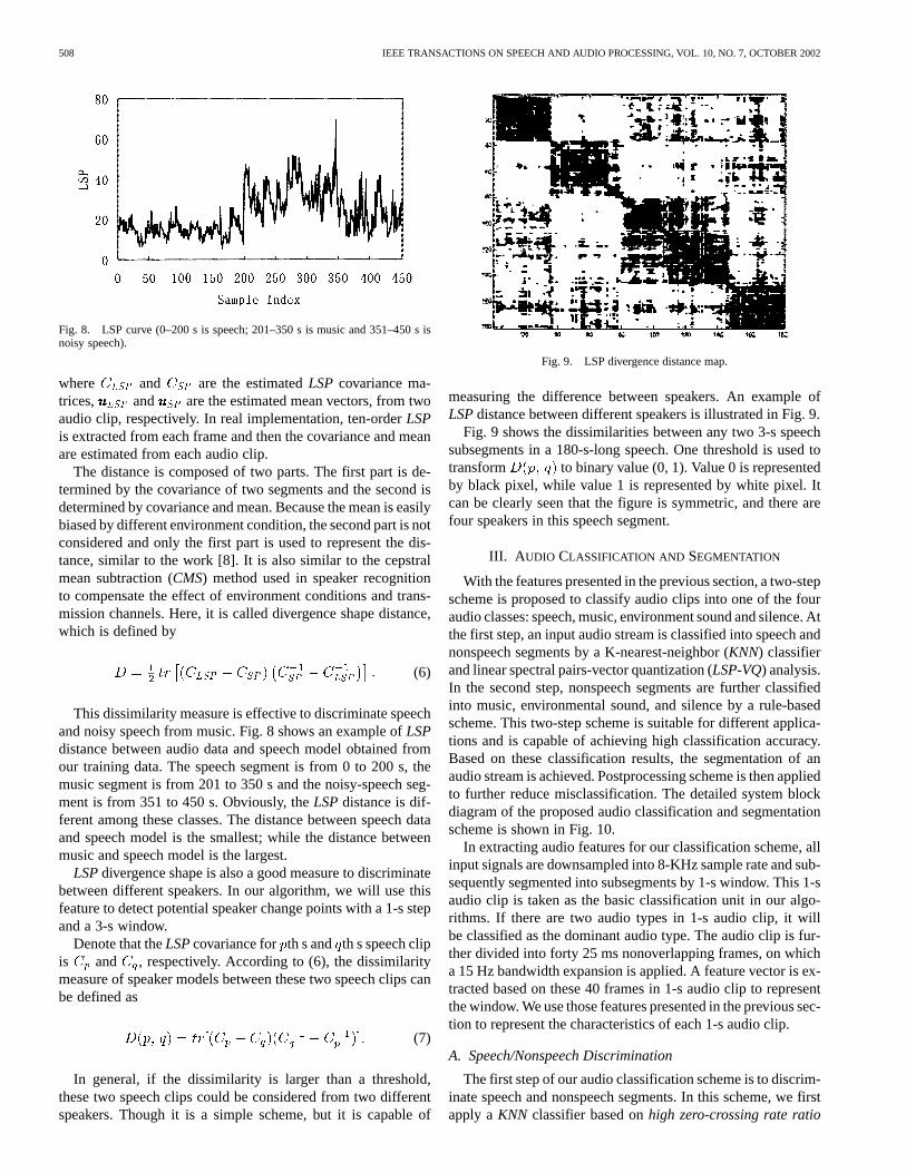
Fig. 8. LSP curve (0–200 s is speech; 201–350 s is music and 351–450 s isnoisy speech).

where LSP and SP are the estimatedLSP covariance ma-trices, LSP and SP are the estimated mean vectors, from twoaudio clip, respectively. In real implementation, ten-orderLSPis extracted from each frame and then the covariance and meanare estimated from each audio clip.

The distance is composed of two parts. The first part is de-termined by the covariance of two segments and the second isdetermined by covariance and mean. Because the mean is easilybiased by different environment condition, the second part is notconsidered and only the first part is used to represent the dis-tance, similar to the work [8]. It is also similar to the cepstralmean subtraction (CMS) method used in speaker recognitionto compensate the effect of environment conditions and trans-mission channels. Here, it is called divergence shape distance,which is defined by

LSP SP SP LSP(6)

This dissimilarity measure is effective to discriminate speechand noisy speech from music. Fig. 8 shows an example ofLSPdistance between audio data and speech model obtained fromour training data. The speech segment is from 0 to 200 s, themusic segment is from 201 to 350 s and the noisy-speech seg-ment is from 351 to 450 s. Obviously, theLSPdistance is dif-ferent among these classes. The distance between speech dataand speech model is the smallest; while the distance betweenmusic and speech model is the largest.

LSPdivergence shape is also a good measure to discriminatebetween different speakers. In our algorithm, we will use thisfeature to detect potential speaker change points with a 1-s stepand a 3-s window.

Denote that theLSPcovariance for th s and th s speech clipis and , respectively. According to (6), the dissimilaritymeasure of speaker models between these two speech clips canbe defined as

(7)

In general, if the dissimilarity is larger than a threshold,these two speech clips could be considered from two differentspeakers. Though it is a simple scheme, but it is capable of

Fig. 9. LSP divergence distance map.

measuring the difference between speakers. An example ofLSPdistance between different speakers is illustrated in Fig. 9.

Fig. 9 shows the dissimilarities between any two 3-s speechsubsegments in a 180-s-long speech. One threshold is used totransform to binary value (0, 1). Value 0 is representedby black pixel, while value 1 is represented by white pixel. Itcan be clearly seen that the figure is symmetric, and there arefour speakers in this speech segment.

III. A UDIO CLASSIFICATION AND SEGMENTATION

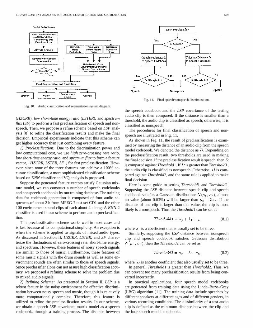
With the features presented in the previous section, a two-stepscheme is proposed to classify audio clips into one of the fouraudio classes: speech, music, environment sound and silence. Atthe first step, an input audio stream is classified into speech andnonspeech segments by a K-nearest-neighbor (KNN) classifierand linear spectral pairs-vector quantization (LSP-VQ) analysis.In the second step, nonspeech segments are further classifiedinto music, environmental sound, and silence by a rule-basedscheme. This two-step scheme is suitable for different applica-tions and is capable of achieving high classification accuracy.Based on these classification results, the segmentation of anaudio stream is achieved. Postprocessing scheme is then appliedto further reduce misclassification. The detailed system blockdiagram of the proposed audio classification and segmentationscheme is shown in Fig. 10.

In extracting audio features for our classification scheme, allinput signals are downsampled into 8-KHz sample rate and sub-sequently segmented into subsegments by 1-s window. This 1-saudio clip is taken as the basic classification unit in our algo-rithms. If there are two audio types in 1-s audio clip, it willbe classified as the dominant audio type. The audio clip is fur-ther divided into forty 25 ms nonoverlapping frames, on whicha 15 Hz bandwidth expansion is applied. A feature vector is ex-tracted based on these 40 frames in 1-s audio clip to representthe window. We use those features presented in the previous sec-tion to represent the characteristics of each 1-s audio clip.

A. Speech/Nonspeech Discrimination

The first step of our audio classification scheme is to discrim-inate speech and nonspeech segments. In this scheme, we firstapply aKNN classifier based onhigh zero-crossing rate ratio


Fig. 10. Audio classification and segmentation system diagram.

(HZCRR), low short-time energy ratio(LSTER), andspectrumflux (SF) to perform a fast preclassification of speech and non-speech. Then, we propose a refine scheme based onLSPanal-ysis [8] to refine the classification results and make the finaldecision. Empirical experiments indicate that this scheme canget higher accuracy than just combining every feature.

1) Preclassification: Due to the discrimination power andlow computational cost, we usehigh zero-crossing rate ratio,low short-time energy ratio,andspectrum fluxto form a featurevector, HZCRR, LSTER, SF , for fast preclassification. How-ever, since none of the three features can achieve a 100% ac-curate classification, a more sophisticated classification schemebased onKNN classifier and VQ analysis is proposed.

Suppose the generated feature vectors satisfy Gaussian mix-ture model, we can construct a number of speech codebooksand nonspeech codebooks by our training database. The trainingdata for codebook generation is composed of four audio se-quences of about 2 h from MPEG-7 test set CD1 and the other100 environment sound clips of each about 4 s long. AKNN-2classifier is used in our scheme to perform audio preclassifica-tion.

This preclassification scheme works well in most cases andis fast because of its computational simplicity. An exception iswhen the scheme is applied to signals of mixed audio types.As discussed in Section II,HZCRR, LSTER, and SF charac-terize the fluctuations of zero-crossing rate, short-time energy,and spectrum. However, these features of noisy speech signalsare similar to those of music. Furthermore, these features ofsome music signals with the drum sounds as well as some en-vironment sounds are often similar to those of speech signals.Since preclassifier alone can not assure high classification accu-racy, we proposed a refining scheme to solve the problem dueto mixed audio signals.

2) Refining Scheme:As presented in Section II,LSP is arobust feature in the noisy environment for effective discrimi-nation between noisy speech and music, though it is relativelymore computationally complex. Therefore, this feature isutilized to refine the preclassification results. In our scheme,we obtain a speechLSPcovariance matrix model as a speechcodebook, through a training process. The distance between

Fig. 11. Final speech/nonspeech discrimination.

the speech codebook and theLSP covariance of the testingaudio clip is then compared. If the distance is smaller than athreshold, the audio clip is classified as speech; otherwise, it isclassified as nonspeech.

The procedures for final classification of speech and non-speech are illustrated in Fig. 11.

As shown in Fig. 11, the result of preclassification is exam-ined by measuring the distance of an audio clip from the speechmodel codebook. We denoted the distance as. Depending onthe preclassification result, two thresholds are used in makingthe final decision. If the preclassification result is speech, thenis compared againstThreshold1. If is greater thanThreshold1,the audio clip is classified as nonspeech. Otherwise,is com-pared againstThreshold2, and the same rule is applied to makefinal decision.

Here is some guide to settingThreshold1 andThreshold2.Supposing theLSP distance between speech clip and speechcodebook satisfies a Gaussian distribution: , almostno value (about 0.03%) will be larger than . If thedistance of one clip is larger than this value, the clip is mostlikely is a nonspeech. Thus theThreshold1 can be set as

Threshold (8.1)

where is a coefficient that is usually set to be three.Similarly, supposing theLSP distance between nonspeech

clip and speech codebook satisfies Gaussian distribution, then theThreshold2 can be set as

Threshold (8.2)

where is another coefficient that also usually set to be three.In general,Threshold1 is greater thanThreshold2. Thus, we

can prevent too many preclassification results from being con-verted incorrectly.

In practical applications, four speech model codebooksare generated from training data using the Linde–Buzo–Gray(LBG) algorithm [11]. The training data include speeches bydifferent speakers at different ages and of different genders, invarious recording conditions. The dissimilarity of a test audioclip is defined as the minimum distance between the clip andthe four speech model codebooks.


B. Music, Environment Sound, and Silence ClassificationScheme

Nonspeech is further classified into music, environmentsound, and silence segments. In our scheme, silence detectionis performed first. Then, for nonsilence segment, it is classifiedinto music or environment sound by applying a set of rules.

1) Detecting Silence:Silence detection is performed basedon short-time energy and zero-crossing rate in 1-s windows. Ifthe average short-time energy and zero-crossing rate is lowerthan a threshold, the segment is classified as silence; otherwise,it is classified as nonsilence segment. This simple scheme workswell in our applications.

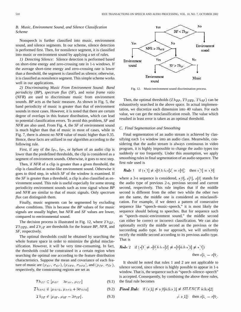
2) Discriminating Music From Environment Sound: Bandperiodicity (BP), spectrum flux(SF), and noise frame ratio(NFR) are used to discriminate music from environmentsounds.BP acts as the basic measure. As shown in Fig. 5, theband periodicity of music is greater than that of environmentsounds in most cases. However, it is noted that there are certaindegree of overlaps in this feature distribution, which can leadto potential classification errors. To avoid this problem,SFandNFRare also used. From Fig. 4, theSFof environment soundis much higher than that of music in most of cases, while inFig. 7, there is almost noNFRvalue of music higher than 0.35.Hence, these facts are utilized in our algorithm according to thefollowing rule.

First, if any of the , , or bpSumof an audio clip islower than the predefined thresholds, the clip is considered as asegment of environment sounds. Otherwise, it goes to next step.

Then, if NFRof a clip is greater than a given threshold, theclip is classified as noise-like environment sound. Otherwise itgoes to third step, in whichSF of the window is examined. IftheSF is greater than a threshold, a clip is also classified as en-vironment sound. This rule is useful especially for some strongperiodicity environment sounds such as tone signal whoseBPand NFR are similar to that of music signals. Onlyspectrumflux can distinguish them.

Finally, music segments can be segmented by excludingabove conditions. This is because theBP values of for musicsignals are usually higher, butNFR andSF values are lower,compared to environmental sound.

The decision process is illustrated in Fig. 12, whereBP ,NFR , and SF are thresholds for the featureBP, NFR, and

SF, respectively.The optimal thresholds could be obtained by searching the

whole feature space in order to minimize the global misclas-sification. However, it will be very time-consuming. In fact,the thresholds could be constrained in a certain region whensearching the optimal one according to the feature distributioncharacteristics. Suppose the mean and covariance of each fea-ture of music are BP BP , NFR NFR , and SF SF ,respectively, the constraining regions are set as

BP BP BP BP (9.1)

NFR NFR NFR NFR (9.2)

SF SF SF SF (9.3)

Fig. 12. Music/environment sound discrimination process.

Then, the optimal thresholds ( BP , NFR , SF can beexhaustively searched in the above space. In actual implemen-tation, we discretize each dimension into 40 values. For eachvalue, we can get the misclassification result. The value whichresulted in least error is taken as an optimal threshold.

C. Final Segmentation and Smoothing

Final segmentation of an audio stream is achieved by clas-sifying each 1-s window into an audio class. Meanwhile, con-sidering that the audio stream is always continuous in videoprogram, it is highly impossible to change the audio types toosuddenly or too frequently. Under this assumption, we applysmoothing rules in final segmentation of an audio sequence. Thefirst rule used is

if then

where a 3-s sequence is considered,, , stands forthe audio type of previous 2-s, previous second and currentsecond, respectively. This rule implies that if the middlesecond is different from the other two while the other twoare the same, the middle one is considered as misclassifi-cation. For example, if we detect a pattern of consecutivesequence like “speech–music–speech,” it is most likely thesequence should belong to speeches. But for sequence suchas “speech–music-environment sound,” the middle secondcan either be correct or incorrect classification. We can alsooptionally rectify the middle second as the previous or thesucceeding audio type. In our approach, we will uniformlyrectify the middle second according to its previous audio type.That is

if

then

It should be noted that rules 1 and 2 are not applicable tosilence second, since silence is highly possible to appear in 1-swindow. That is, the sequence such as “speech–silence–speech”is accepted. Consequently, by combining the above three rules,the final rule becomes

if SILENCE

then


Fig. 13. Flow diagram for speaker change detection.

IV. SPEAKER SEGMENTATION

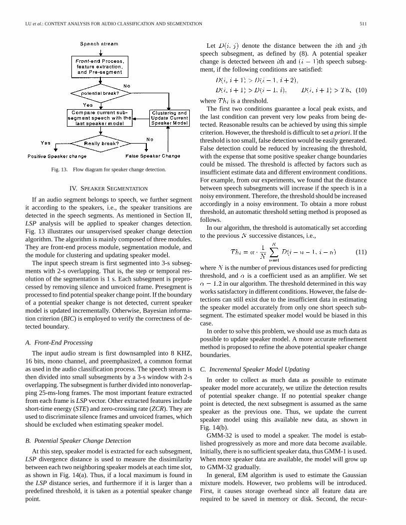
If an audio segment belongs to speech, we further segmentit according to the speakers, i.e., the speaker transitions aredetected in the speech segments. As mentioned in Section II,LSP analysis will be applied to speaker changes detection.Fig. 13 illustrates our unsupervised speaker change detectionalgorithm. The algorithm is mainly composed of three modules.They are front-end process module, segmentation module, andthe module for clustering and updating speaker model.

The input speech stream is first segmented into 3-s subseg-ments with 2-s overlapping. That is, the step or temporal res-olution of the segmentation is 1 s. Each subsegment is prepro-cessed by removing silence and unvoiced frame. Presegment isprocessed to find potential speaker change point. If the boundaryof a potential speaker change is not detected, current speakermodel is updated incrementally. Otherwise, Bayesian informa-tion criterion (BIC) is employed to verify the correctness of de-tected boundary.

A. Front-End Processing

The input audio stream is first downsampled into 8 KHZ,16 bits, mono channel, and preemphasized, a common formatas used in the audio classification process. The speech stream isthen divided into small subsegments by a 3-s window with 2-soverlapping. The subsegment is further divided into nonoverlap-ping 25-ms-long frames. The most important feature extractedfrom each frame isLSPvector. Other extracted features includeshort-time energy (STE) and zero-crossing rate (ZCR). They areused to discriminate silence frames and unvoiced frames, whichshould be excluded when estimating speaker model.

B. Potential Speaker Change Detection

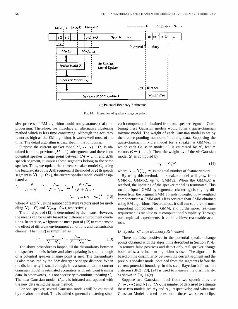
At this step, speaker model is extracted for each subsegment,LSP divergence distance is used to measure the dissimilaritybetween each two neighboring speaker models at each time slot,as shown in Fig. 14(a). Thus, if a local maximum is found inthe LSP distance series, and furthermore if it is larger than apredefined threshold, it is taken as a potential speaker changepoint.

Let denote the distance between theth and thspeech subsegment, as defined by (8). A potential speakerchange is detected betweenth and th speech subseg-ment, if the following conditions are satisfied:

(10)

where is a threshold.The first two conditions guarantee a local peak exists, and

the last condition can prevent very low peaks from being de-tected. Reasonable results can be achieved by using this simplecriterion. However, the threshold is difficult to seta priori. If thethreshold is too small, false detection would be easily generated.False detection could be reduced by increasing the threshold,with the expense that some positive speaker change boundariescould be missed. The threshold is affected by factors such asinsufficient estimate data and different environment conditions.For example, from our experiments, we found that the distancebetween speech subsegments will increase if the speech is in anoisy environment. Therefore, the threshold should be increasedaccordingly in a noisy environment. To obtain a more robustthreshold, an automatic threshold setting method is proposed asfollows.

In our algorithm, the threshold is automatically set accordingto the previous successive distances, i.e.,

(11)

where is the number of previous distances used for predictingthreshold, and is a coefficient used as an amplifier. We set

in our algorithm. The threshold determined in this wayworks satisfactory in different conditions. However, the false de-tections can still exist due to the insufficient data in estimatingthe speaker model accurately from only one short speech sub-segment. The estimated speaker model would be biased in thiscase.

In order to solve this problem, we should use as much data aspossible to update speaker model. A more accurate refinementmethod is proposed to refine the above potential speaker changeboundaries.

C. Incremental Speaker Model Updating

In order to collect as much data as possible to estimatespeaker model more accurately, we utilize the detection resultsof potential speaker change. If no potential speaker changepoint is detected, the next subsegment is assumed as the samespeaker as the previous one. Thus, we update the currentspeaker model using this available new data, as shown inFig. 14(b).

GMM-32 is used to model a speaker. The model is estab-lished progressively as more and more data become available.Initially, there is no sufficient speaker data, thus GMM-1 is used.When more speaker data are available, the model will grow upto GMM-32 gradually.

In general, EM algorithm is used to estimate the Gaussianmixture models. However, two problems will be introduced.First, it causes storage overhead since all feature data arerequired to be saved in memory or disk. Second, the recur-


Fig. 14. Illustration of speaker change detection.

sive process of EM algorithm could not guarantee real-timeprocessing. Therefore, we introduce an alternative clusteringmethod which is less time consuming. Although the accuracyis not as high as the EM algorithm, it works well most of thetime. The detail algorithm is described in the following.

Suppose the current speaker model is ob-tained from the previous subsegments and there is nopotential speaker change point between th and thspeech segment, it implies these segments belong to the samespeaker. Thus, we update the current speaker modelusingthe feature data of the th segment. If the model of th speechsegment is , the current speaker model could be up-dated as

(12)

where and is the number of feature vectors used for mod-eling and , respectively.

The third part of (12) is determined by the means. However,the means can be easily biased by different environment condi-tions. In practice, we ignore the mean part of (12) to compensatethe effect of different environment conditions and transmissionchannel. Then, (12) is simplified as

(13)

The above procedure is looped till the dissimilarity betweenthe speaker models before and after updating is small enoughor a potential speaker change point is met. The dissimilarityis also measured by theLSPdivergence shape distance. Whenthe dissimilarity is small enough, it is assumed that the currentGaussian model is estimated accurately with sufficient trainingdata. In other words, it is not necessary to continue updating.The next Gaussian model, , is initiated and updated withthe new data using the same method.

For one speaker, several Gaussian models will be estimatedby the above method. This is called segmental clustering since

each component is obtained from one speaker segment. Com-bining these Gaussian models would form a quasi-Gaussianmixture model. The weight of each Gaussian model is set bytheir corresponding number of training data. Supposing thequasi-Gaussian mixture model for a speaker is GMM-s, inwhich each Gaussian model is estimated by featurevectors ( ). Then, the weight of the th Gaussianmodel is computed by

(14)

where is the total number of feature vectors.By using this method, the speaker model will grow from

GMM-1, GMM-2, up to GMM32. When the GMM32 isreached, the updating of the speaker model is terminated. Thismethod (quasi-GMM by segmental clustering) is slightly dif-ferent from the original GMM. It tends to neglect low-weightedcomponents in a GMM and is less accurate than GMM obtainedusing EM algorithms. Nevertheless, it still can capture the mostimportant components in GMM, and furthermore, real-timerequirement is met due to its computational simplicity. Throughour empirical experiments, it could achieve reasonable accu-racy.

D. Speaker Change Boundary Refinement

There are false positives in the potential speaker changepoints obtained with the algorithms described in Section IV-B.To remove false positives and detect only real speaker changeboundaries, a refinement algorithm is used. The algorithm isbased on the dissimilarity between the current segment and theprevious speaker model obtained from the segments before thecurrent potential boundary. In this step, Bayesian informationcriterion (BIC) [23], [24] is used to measure the dissimilarity,as shown in Fig. 14(c).

Suppose two Gaussian model from two speech clips areand , the number of data used to estimate

these two models are and , respectively; and when oneGaussian Model is used to estimate these two speech clips,


the model is . The BIC difference between the twomodels is

(15)

where is a penalty factor to compensated for small size cases,and is the feature dimension. Generally, .

According to BIC theory, ifBIC is positive, thetwo speech clips could be considered from different sources(speakers). The advantage of using BIC is that it is thresholdfree.

Suppose at the potential speaker boundary, the model ofprevious speaker is GMM-s, in which each Gaussian model is

; and the model of current segmentis . Then the distance between them is estimated asthe weighted sum of the distance between and each

BIC (16)

This distance does not take the GMM-s as an integral one,but as several independent components. However, it is still rea-sonable since the GMM-s model is obtained from segmentalclustering. That is, each component Gaussian model is obtainedfrom an independent segment. The BIC distance consideringone component of GMM-s can be used as the similarity confi-dence between the current segment and one segment of the pre-vious speaker. Thus, the weighted sum (average distance) canbe used to represent the distance between current segment andprevious speaker.

Based on the aforementioned BIC theory, if , it mustbe a real speaker change boundary. If a candidate is not a realboundary, the speaker data is used to update the speaker modelfollowing the method previously described.

LSP divergence distance or Bayesian information criterionis not uniformly used at potential speaker boundary detectionand refinement. The reason is as follows. At the step of poten-tial speaker change detection, the data is too small to estimatea model accurately. Bayesian information criterion is found tobe vulnerable by different words or different speakers, so falsealarms can be easily generated. At the step of potential boundaryrefining, the model is more accurate; moreover, BIC could com-pensate different training data and is threshold free, whileLSPdivergence distance depends on thresholds. It is more efficientfor BIC in this step, as shown in our experiments.

V. EXPERIMENT RESULTS

A. Audio Classification and Segmentation Evaluations

The evaluation of the proposed audio classification and seg-mentation algorithms have been performed by using an audiodatabase composing of data from MPEG-7 test data set CD1, TVnews, movie clips, and some audio clips from the Internet. Thisdatabase includes speech in various conditions, such as in recordstudios, speeches with telephone (4 kHz) bandwidth and 8 kHz

TABLE ISPEECH, MUSIC, ENVIRONMENT SOUND CLASSIFICATION ON

BASELINE SYSTEM (UNIT: 100%)

TABLE IIBASELINE CLASSIFICATION RESULT ON PURE SPEECH AND

NOISY SPEECH(UNIT: 100%)

TABLE IIICLASSIFICATION ON PURE SPEECH AND NOISY SPEECH

AFTER REFINEMENT (UNIT: 100%)

bandwidth. The music content in this data set is mainly songsand pop music. Such music contents are difficult for most audioclassifiers. The background sound in the database include manytypes, such as aviations, animals, autos, beeps, cartoon, combat,crowds, and so on. Two hours of data was used for training, and4-h data was used for testing. The testing data includes about9600 s speech, 3400 s music, and 1200 s environment sounds.The training data is approximately half of the testing data. In ourexperiments, we set 1 s as a test unit. If there are two audio typesin a 1-s audio clip, we will classify it as the dominant audio type.

We first implement a baseline system which uses the feature(HZCRR, LSTER, SF) with clustering and the NNmethod, asdescribed in the Section III. The performance data are listed inTable I.

This baseline system works well for speech/nonspeech dis-crimination, but does not work well on environment sound. Inour experiments, we also found that the baseline system hasworse performance on noisy speech than pure speech. About26.38% noisy speech is discriminated as music, as shown in theTable II. This is because some features of noisy speech are verysimilar to those of music, in particular the pop music.

These facts show that the base system is only effective as apreclassification process, and more improvements are expected.Therefore, we propose to use new features to increase the clas-sification performance of noisy speech and environment sound.After the refinement scheme byLSPdivergence shape, the per-formance is improved significantly, as shown in Table III.

After employing our music and environment classificationscheme, the performance for environment classification is also


TABLE IVSPEECH, MUSIC, ENVIRONMENT SOUND CLASSIFICATION

BEFORESMOOTHING (UNIT: 100%)

TABLE VFINAL RESULT OF SPEECH, MUSIC, ENVIRONMENT SOUND

CLASSIFICATION (UNIT: 100%)

TABLE VITHE TOTAL ACCURACY RESULT FORDIFFERENTDISCRIMINATION TYPE

improved. The total performance of our system is showed inTable IV.

Considering the continuity of audio stream, a smoothingscheme is processed. The performance has been further im-proved as shown in Table V.

From Table V, we can see that speech, music, and environ-ment sound can be well discriminated. 97.45% of speech sam-ples are discriminated correctly; only 1.55% speech is mistak-enly classified into music while 1.00% into environment sounds.The total accuracy of discriminating these three classes is ashigh as 96.51%. If only speech and music are considered, theaccuracy reaches 98.03%. The final accuracy results of differentdiscrimination types are listed in Table VI.

The experiments have shown that the proposed schemeachieves excellent classification accuracy.

B. Speaker Change Detection and Segmentation Evaluation

The testing materials used for speaker segmentation evalu-ations are news video programs from MPEG7 test data, CNNnews, and CCTV news. In total, they are about 2 h. The audiotrack in the test set is sampled at 16 kHz, 32 kHz, or 44.1 kHzin one or two channels. In the experiments, each format audio isconverted to 8 kHz and mono-channel before further processing.

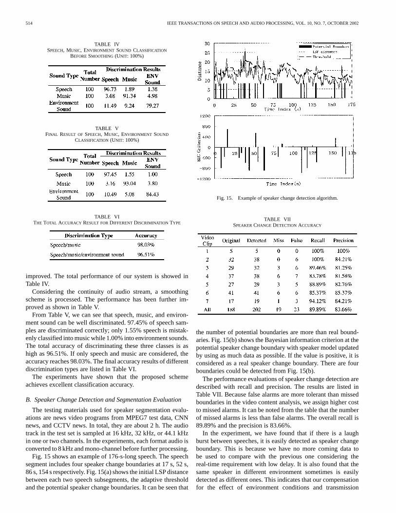
Fig. 15 shows an example of 176-s-long speech. The speechsegment includes four speaker change boundaries at 17 s, 52 s,86 s, 154 s respectively. Fig. 15(a) shows the initial LSP distancebetween each two speech subsegments, the adaptive thresholdand the potential speaker change boundaries. It can be seen that

Fig. 15. Example of speaker change detection algorithm.

TABLE VIISPEAKER CHANGE DETECTION ACCURACY

the number of potential boundaries are more than real bound-aries. Fig. 15(b) shows the Bayesian information criterion at thepotential speaker change boundary with speaker model updatedby using as much data as possible. If the value is positive, it isconsidered as a real speaker change boundary. There are fourboundaries could be detected from Fig. 15(b).

The performance evaluations of speaker change detection aredescribed with recall and precision. The results are listed inTable VII. Because false alarms are more tolerant than missedboundaries in the video content analysis, we assign higher costto missed alarms. It can be noted from the table that the numberof missed alarms is less than false alarms. The overall recall is89.89% and the precision is 83.66%.

In the experiment, we have found that if there is a laughburst between speeches, it is easily detected as speaker changeboundary. This is because we have no more coming data tobe used to compare with the previous one considering thereal-time requirement with low delay. It is also found that thesame speaker in different environment sometimes is easilydetected as different ones. This indicates that our compensationfor the effect of environment conditions and transmission


channel is insufficient. The problem would remain a challengein the speaker recognition field and may have a long way to go.

C. Computation Complexity

We have also tested the computational complexity of our al-gorithm in term of CPU time. With a Pentium III 667 MHz PCwith Windows 2000, the whole process, including audio seg-mentation and speaker segmentation, can be completed in about20% of the length of an audio/video clip. The correlation calcu-lation in computingLSPmatrix and band periodicity is the mosttime-consuming part in our algorithm. After using an optimizedfunction to compute these features, the time performance hasbeen increased dramatically. Therefore, our audio classificationand speaker segmentation scheme is able to meet the real-timerequirement in multimedia applications.

VI. CONCLUSIONS

In this paper, we have presented our study on audio classifi-cation and segmentation for applications in audio/video contentanalysis. We have described in detail a novel audio segmenta-tion and classification scheme that segments and classifies anaudio stream into speech, music, environment sound, and si-lence. These classes are the basic data set for audio/video con-tent analysis. The algorithm has been developed and presentedin two stages, which is very suitable for different applications.We also have introduced a set of new features, such asnoiseframe ratioandband periodicity, which have high discrimina-tion power among different audio types. Experimental evalua-tion has shown that the proposed audio classification scheme isvery effective and the total accuracy rate is over 96%. The novelscheme and new features introduced ensure that the system canachieve high accuracy even with a smaller testing unit.

We have also developed an improved approach on unsuper-vised speaker segmentation based onLSPdivergence analysis.Incremental speaker modeling and adaptive threshold settinghave been described in detail, which makes unsupervisedspeaker segmentation possible. Segmental clustering, whichrequires less computation, has also been proposed, so that thealgorithm can totally suit the real-time processing in multi-media application. Experiments have shown that the algorithmis considerably effective. The overall recall is up to 89.89%,and the precision is 83.66%.

In the future, our audio classification scheme will be im-proved to discriminate more audio classes. We will improve theperformance of our speaker segmentation algorithm and extendit to speaker tracking. We will also focus on developing an ef-fective scheme to apply audio content analysis to assist videocontent analysis and indexing.

REFERENCES

[1] J. Foote, “Content-based retrieval of music and audio,”Proc. SPIE, vol.3229, pp. 138–147, 1997.

[2] E. Wold, T. Blum, and J. Wheaton, “Content-based classification, searchand retrieval of audio,”IEEE Multimedia, vol. 3, no. 3, pp. 27–36, 1996.

[3] S. Pfeiffer, S. Fischer, and W. Effelsberg, “Automatic audio content anal-ysis,” in Proc. 4th ACM Int. Conf. Multimedia, 1996, pp. 21–30.

[4] J. Saunders, “Real-time discrimination of broadcast speech/music,” inProc. ICASSP’96, vol. II, Atlanta, GA, May 1996, pp. 993–996.

[5] E. Scheirer and M. Slaney, “Construction and evaluation of a robust mul-tifeature music/speech discriminator,” inProc. ICASSP’ 97, Apr. 1997,vol. II, pp. 1331–1334.

[6] D. Kimber and L. Wilcox, “Acoustic segmentation for audio browsers,”in Proc. Interface Conf., Sydney, Australia, July 1996.

[7] T. Zhang and C.-C. J. Kuo, “Video content parsing based on combinedaudio and visual information,”Proc. SPIE, vol. IV, pp. 78–89, 1992.

[8] J. P. Campbell, Jr., “Speaker recognition: A tutorial,”Proc. IEEE, vol.85, no. 9, pp. 1437–1462, 1997.

[9] A. V. McCree and T. P. Barnwell, “Mixed excitation LPC Vocoder modelfor low bit rate speech coding,” inIEEE Trans. Speech Audio Processing,July 1995, vol. 3, pp. 242–250.

[10] K. El-Maleh, M. Klein, G. Petrucci, and P. Kabal, “Speech/music dis-crimination for multimedia application,” inProc. ICASSP’00, 2000.

[11] Y. Linde, A. Buzo, and R. M. Gray, “A algorithm for vector quantizerdesign,”IEEE Trans. Commun., vol. COM-28, no. 1, pp. 84–95, 1980.

[12] S. Srinivasan, D. Petkovic, and D. Ponceleon, “Toward robust featuresfor classifying audio in the CueVideo system,” inProc. 7th ACM Int.Conf. Multimedia, 1999, pp. 393–400.

[13] Z. Liu, Y. Wang, and T. Chen, “Audio feature extraction and analysisfor scene segmentation and classification,”J. VLSI Signal Process. Syst.,June 1998.

[14] L. Lu, H. Jiang, and H. J. Zhang, “A robust audio classification andsegmentation method,” inProc. 9th ACM Int. Conf. Multimedia, 2001,pp. 203–211.

[15] J. S. Boreczky and L. D. Wilcox, “A hidden Markov model framework for video segmentation using audio and image features,” inProc.ICASSP’98, Seattle, WA, May 1998, pp. 3741–3744.

[16] J. N. L. Brummer, “Speaker recognition over HF radio after automaticspeaker segmentation,” inProc. IEEE South African Symp. Communi-cations and Signal Processing (COMSIG-94), 1994, pp. 171–176.

[17] M. Sugiyama, J. Murakami, and H. Watanabe, “Speech segmentationand clustering based on speaker features,” inProc. IEEE Int. Conf.Acoustics, Speech, Signal Processing, 1993.

[18] L. Wilcox, F. Chen, D. Kumber, and V. Balasubramanian, “Segmenta-tion of speech using speaker identification,” inProc. IEEE Int. Conf.Acoustics, Speech, Signal Processing, 1994.

[19] M. H. Siu, G. Yu, and H. Gish, “An unsupervised, sequential learningalgorithm for the segmentation of speech waveform with multiplespeakers,” inProc. IEEE Int. Conf. Acoustics, Speech, Signal Pro-cessing, 1992, pp. 189–192.

[20] H. Gish, M. H. Siu, and R. Rohlicek, “Segregation of speakers for speechrecognition and speaker identification,” inProc. ICASSP’91, 1991, pp.873–876.

[21] A. Cohen and V. Lapidus, “Unsupervised speaker segmentation in tele-phone conversations,” inProc. 19th Conv. Electrical Electronics Engi-neers in Israel, 1996, pp. 102–105.

[22] K. Mori and S. Nakagawa, “Speaker change detection and speaker clus-tering using VQ distortion for broadcast news speech recognition,” inProc. ICASSP’01, vol. I, 2001, pp. 413–416.

[23] S. Chen and P. S. Gopalakrishnan, “Speaker, environment and channelchange detection and clustering via the Bayesian information criterion,”in Proc. DARPA Broadcast News Transcription and UnderstandingWorkshop, 1998.

[24] G. Schwarz, “Estimation the dimension of a model,”Ann. Statist., vol.6, pp. 461–464, 1978.

Lie Lu received his B.S. and M.S. from ShanghaiJiao Tong University, China, both in electrical engi-neering, in 1997 and 2000, respectively.

In 2000, he joined Microsoft Research Asia, Bei-jing, China, where he is currently an Associate Re-searcher with the Media Computing Group. His cur-rent interests are in the areas of pattern recognition,content-based audio analysis, and music analysis.


Hong-Jiang Zhang (S’90–M’91–SM’97) receivedthe Ph.D. degree from the Technical Universityof Denmark and the B.S. degree from ZhengzhouUniversity, China, both in electrical engineering, in1982 and 1991, respectively.

From 1992 to 1995, he was with the Institute ofSystems Science, National University of Singapore,where he led several projects in video and imagecontent analysis and retrieval and computer vision.He also worked at Massachusetts Institute ofTechnology Media Lab, Cambridge, MA, in 1994

as a Visiting Researcher. From 1995 to 1999, he was a Research Manager atHewlett-Packard Labs, where he was responsible for research and technologytransfers in the areas of multimedia management; intelligent image processingand Internet media. In 1999, he joined Microsoft Research Asia, where heis currently a Senior Researcher and Assistant Managing Director in chargeof media computing and information processing research. He has authoredthree books, over 200 referred papers and book chapters, seven specialissues of international journals on image and video processing, content-basedmedia retrieval, and computer vision, as well as numerous patents or pendingapplications.

Dr. Zhang is a member of ACM. He currently serves on the editorial boards offive IEEE/ACM journals and a dozen committees of international conferences.

Hao Jiang received the Ph.D. in electronic engi-neering from Tsinghua University, Beijing, in 1999.He received the B.S. and M.S. degrees in electronicengineering from Harbin Engineering University,Harbin, China, in 1993 and 1995, respectively. Heis currently pursuing the Ph.D. degree in computingscience in Simon Fraser University, Vancouver, BC,Canada.

He had been an Associate Researcher withMicrosoft Research Asia, Beijing, from 1999 to2000. His current research interest is on multimedia,

image and video processing, computer vision, and computer graphics.

Documents

Content analysis for audio classification and segmentation - Speech · PDF file · 2017-03-22segmenting an audio stream into speech, music, environment sound, ... works on audio content