Embed Size (px)
Citation preview
Contact Geometry of the Visual Cortex
Matilde Marcolli and Doris Tsao
Ma191b Winter 2017Geometry of Neuroscience
Matilde Marcolli and Doris Tsao Contact Geometry of the Visual Cortex

References for this lecture
Jean Petitot, Neurogeometrie de la Vision, Les Editions del’Ecole Polytechnique, 2008
John B. Entyre, Introductory Lectures on Contact Geometry,arXiv:math/0111118
W.C. Hoffman, The visual cortex is a contact bundle, AppliedMathematics and Computation, 32 (1989) 137–167.
O. Ben-Shahar, S. Zucker, Geometrical Computations ExplainProjection Patterns of Long-Range Horizontal Connections inVisual Cortex, Neural Computation, 16, 3 (2004) 445–476
Alessandro Sarti, Giovanna Citti, Jean Petitot, Functionalgeometry of the horizontal connectivity in the primary visualcortex, Journal of Physiology - Paris 103 (2009) 3–45
Matilde Marcolli and Doris Tsao Contact Geometry of the Visual Cortex
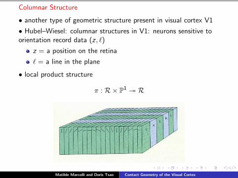
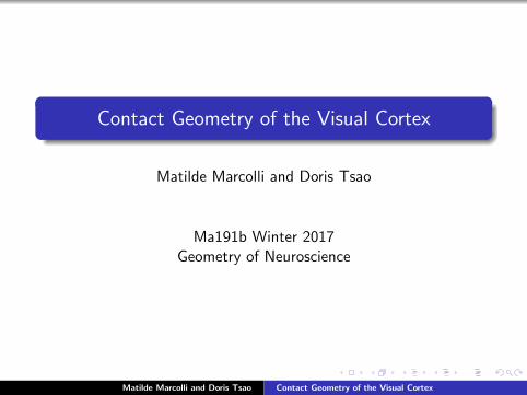
Columnar Structure
• another type of geometric structure present in visual cortex V1
• Hubel–Wiesel: columnar structures in V1: neurons sensitive toorientation record data (z , `)
z = a position on the retina
` = a line in the plane
• local product structure
π : R× P1 � R
Matilde Marcolli and Doris Tsao Contact Geometry of the Visual Cortex
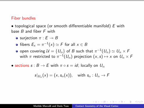
Fiber bundles
• topological space (or smooth differentiable manifold) E withbase B and fiber F with
surjection π : E � B
fibers Ex = π−1(x) ' F for all x ∈ B
open covering U = {Uα} of B such that π−1(Uα) ' Uα × Fwith π restricted to π−1(Uα) projection (x , s) 7→ x on Uα × F
• sections s : B → E with π ◦ s = id ; locally on Uα
s|Uα(x) = (x , sα(x)), with sα : Uα → F
Matilde Marcolli and Doris Tsao Contact Geometry of the Visual Cortex

trivial and nontrivial R-bundles over S1
Matilde Marcolli and Doris Tsao Contact Geometry of the Visual Cortex
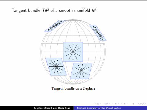
Tangent bundle TM of a smooth manifold M
Matilde Marcolli and Doris Tsao Contact Geometry of the Visual Cortex
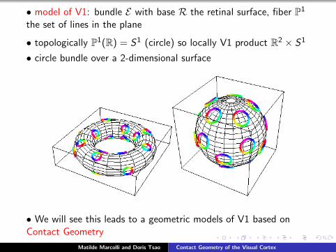
• model of V1: bundle E with base R the retinal surface, fiber P1
the set of lines in the plane
• topologically P1(R) = S1 (circle) so locally V1 product R2 × S1
• circle bundle over a 2-dimensional surface
• We will see this leads to a geometric models of V1 based onContact Geometry
Matilde Marcolli and Doris Tsao Contact Geometry of the Visual Cortex
Contact Geometry on 3-dimensional manifolds
• plane field ξ on 3-manifold M: subbundle of tangent bundle TMsuch that ξx = TxM ∩ ξ is 2-dimensional subspace for all x ∈ M
• Example: M = Σ× S1 product of a 2-dimensional surface Σ anda circle S1, then ξ(x ,θ) = TxΣ ⊂ T(x ,θ)M is a plane field
• real 1-form α on M determines at each point x ∈ M a linear map
αx : TxM → R
Kernel ker(αx) is either a plane or all of TxMif ker(αx) 6= TxM for all x ∈ M then ξ = ker(α) is a plane field
• all plane fields locally given by ξ = ker(α) for some 1-form α
• Example: M = Σ× S1 as above: ξ = ker(α) with α = dθ
Matilde Marcolli and Doris Tsao Contact Geometry of the Visual Cortex

• plane field ξ = ker(α) on 3-manifold M is contact structure iff
α ∧ dα 6= 0
equivalent condition dα|ξ 6= 0
• Standard Example: M = R3 with
α = dz + xdy
so dα = dx ∧ dy and α ∧ dα = dz ∧ dx ∧ dy 6= 0
• at a point (x , y , z) contact plane ξ(x ,y ,z) spanned by basis
{ ∂∂x, x
∂
∂z− ∂
∂y}
• geometry of contact plane field ξ: when x = 0 (yz-plane) contact plane
horizontal; at (1, 0, 0) spanned by ∂∂x ,
∂∂z −
∂∂y , tangent to x-axis, but
tilted 45% clockwise, etc. start at origin and move along x-axis, plane
keeps twisting clockwise
Matilde Marcolli and Doris Tsao Contact Geometry of the Visual Cortex

the standard contact structure on R3
Matilde Marcolli and Doris Tsao Contact Geometry of the Visual Cortex

Darboux’s Theorem
• locally all contact structures look like the standard one
• (M, ξ) and (N, η) contact 3-manifolds, contactomorphism isdiffeomorphism f : M → N such that f∗(ξ) = η; in terms of1-forms f ∗(αη) = hαξ for some non-zero h : M → R• (M, ξ) contact 3-manifold, point x ∈ M, there are neighborhoodsN of x and U of (0, 0, 0) in R3 and contactomorphism
f : (N , ξ|N )→ (U , ξ0|U )
with ξ0 the standard contact structure on R3
Matilde Marcolli and Doris Tsao Contact Geometry of the Visual Cortex

Example: contact structure on sphere S3
• f (x1, y1, x2, y2) = x21 + y2
1 + x22 + y2
2 with S3 = f −1(1) ⊂ R4
• tangent spaces T(x1,y1,x2,y2)S3 = kerdf(x1,y1,x2,y2) =
ker(2x1dx1 + 2y1dy1 + 2x2dx2 + 2y2dy2)
• identify R4 = C2 with complex structure Jxi = yi and Jyi = −xi
J∂
∂xi=
∂
∂yi, J
∂
∂yi= − ∂
∂xi
• contact structure on S3
α = (x1dy1 − y1dx1 + x2dy2 − y2dx2)|S3
α ∧ dα 6= 0
ξ = ker(α) contact planes
Matilde Marcolli and Doris Tsao Contact Geometry of the Visual Cortex
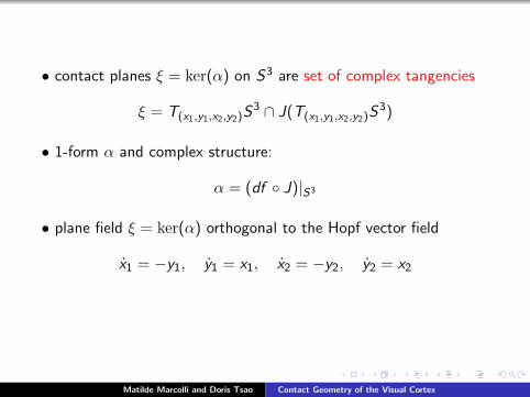
• contact planes ξ = ker(α) on S3 are set of complex tangencies
ξ = T(x1,y1,x2,y2)S3 ∩ J(T(x1,y1,x2,y2)S
3)
• 1-form α and complex structure:
α = (df ◦ J)|S3
• plane field ξ = ker(α) orthogonal to the Hopf vector field
x1 = −y1, y1 = x1, x2 = −y2, y2 = x2
Matilde Marcolli and Doris Tsao Contact Geometry of the Visual Cortex
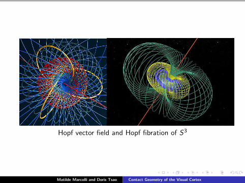
Hopf vector field and Hopf fibration of S3
Matilde Marcolli and Doris Tsao Contact Geometry of the Visual Cortex
Contact Structures and Complex Manifolds
• X complex manifold dimC(X ) = 2 with boundary ∂X , withdimR ∂X = 3, and complex structure J on TX ; function φ nearboundary with ∂X = φ−1(0) (collar neighborhood of boundary)
• complex tangenciesker(dφ ◦ J)
contact structure iff d(dφ ◦ J) non-degenerate 2-form on planes ξ
• contact structure is fillable if obtained in this way
• Lutz–Martinet theorem: all 3-manifolds admit a contactstructure (not always fillable)
Matilde Marcolli and Doris Tsao Contact Geometry of the Visual Cortex
Contact Geometry and Symplectic Geometry
• X real 4-dimensional manifold (or more generally evendimensional); symplectic structure on X : closed 2-form ω suchthat ω ∧ ω 6= 0 (or in dimension 2n form ∧nω 6= 0)
• Darboux’s Theorem for symplectic forms: locally ω = dp ∧ dq(like a cotangent bundle)
• (X , ω) symplectic filling of contact 3-manifold (M, ξ) if ∂X = Mand ω|ξ 6= 0 area form on contact planes
• fillability by complex manifold special case: ω = d(dφ ◦ J) issymplectic
• not all contact structures are fillable by symplectic structures: ifa contact structure is symplectically fillable then it is tight
[Note: can always extend to symplectic on cylinder X = M × Rwith ω = dα + α ∧ dt but not M = ∂X ]
Matilde Marcolli and Doris Tsao Contact Geometry of the Visual Cortex
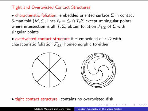
Tight and Overtwisted Contact Structures
• characteristic foliation: embedded oriented surface Σ in contact3-manifold (M, ξ), lines `x = ξx ∩ TxΣ except at singular pointswhere intersection is all TxΣ; obtain foliation Fξ,Σ of Σ withsingular points
• overtwisted contact structure if ∃ embedded disk D withcharacteristic foliation Fξ,D homeomorphic to either
• tight contact structure: contains no overtwisted disk
Matilde Marcolli and Doris Tsao Contact Geometry of the Visual Cortex
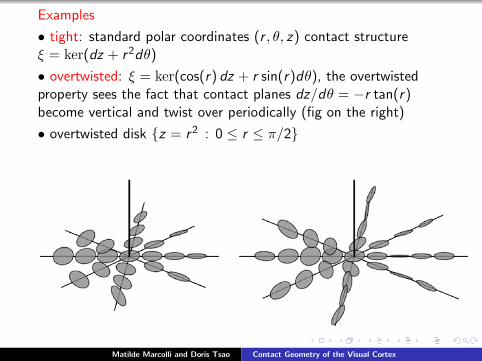
Examples
• tight: standard polar coordinates (r , θ, z) contact structureξ = ker(dz + r2dθ)
• overtwisted: ξ = ker(cos(r) dz + r sin(r)dθ), the overtwistedproperty sees the fact that contact planes dz/dθ = −r tan(r)become vertical and twist over periodically (fig on the right)
• overtwisted disk {z = r2 : 0 ≤ r ≤ π/2}
Matilde Marcolli and Doris Tsao Contact Geometry of the Visual Cortex
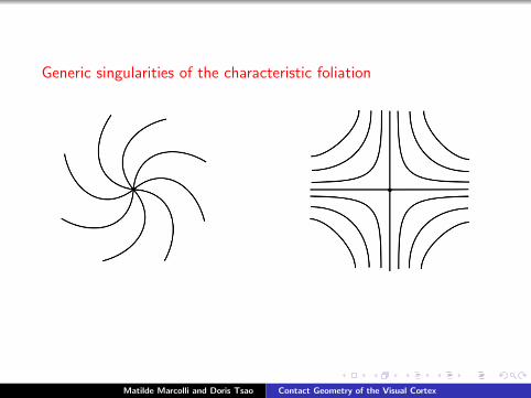
Generic singularities of the characteristic foliation
Matilde Marcolli and Doris Tsao Contact Geometry of the Visual Cortex
Some facts about contact structures and 3-manifolds(Eliashberg, Gromov, Entyre, Honda, Bennequin, etc.)
All 3-manifolds admit contact structures
Some 3-manifolds do not admit any tight contact structure(though most of them do)
If a contact structure is symplectically fillable then it is tight
contact plane field ξ has an Euler class e(ξ) ∈ H2(M,Z): iftight then genus bound
|e(ξ)[Σ]| ≤ −χ(Σ)
if Σ 6= S2 and zero otherwise (key idea: express in terms ofsingular points of the characteristic foliation, Poincare–Hopf)
Matilde Marcolli and Doris Tsao Contact Geometry of the Visual Cortex
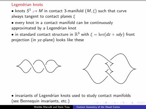
Legendrian knots
• knots S1 ↪→ M in contact 3-manifold (M, ξ) such that curvealways tangent to contact planes ξ
• every knot in a contact manifold can be continuouslyapproximated by a Legendrian knot
• in standard contact structure in R3 with ξ = ker(dz + xdy) frontprojection (in yz-plane) looks like these
• invariants of Legendrian knots used to study contact manifolds(see Bennequin invariants, etc.)
Matilde Marcolli and Doris Tsao Contact Geometry of the Visual Cortex

Transverse knots
• knots S1 ↪→ M in contact 3-manifold (M, ξ) such that curvealways transverse to the contact planes ξ
• for standard contact structure projections of transverse knots inthe xz-planes cannot have segments like
because z ′(t)− y(t)x ′(t) > 0 along a tranverse knot and verticaltangency would have x ′ = 0 and z ′ < 0, while second case y(t)bounded by slope z ′(t)/x ′(t) in xz-plane
• any transverse knot in the standard contact structure istransversely isotopic to a closed braid
Matilde Marcolli and Doris Tsao Contact Geometry of the Visual Cortex
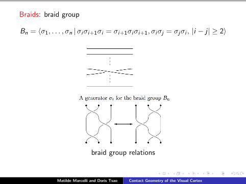
Braids: braid group
Bn = 〈σ1, . . . , σn |σiσi+1σi = σi+1σiσi+1, σiσj = σjσi , |i − j | ≥ 2〉
braid group relations
Matilde Marcolli and Doris Tsao Contact Geometry of the Visual Cortex
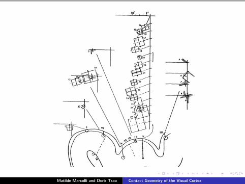
Visual Cortex as Contact Bundle
• W.C. Hoffman, The visual cortex is a contact bundle, AppliedMathematics and Computation, 32 (1989) 137–167
• Hubel–Wiesel microcolumns in columnar structure of V1 cortexexhibit both directional and areal response: model directional-arealresponse fields as contact planes directions
• “orientation response” refers to directionally sensitive responsefield of a single cortical neuron
• microelectrodes penetration measurements of directional andarea response of neurons in the cat visual cortex show contactplanes (Hubel, Wiesel)
Matilde Marcolli and Doris Tsao Contact Geometry of the Visual Cortex
Matilde Marcolli and Doris Tsao Contact Geometry of the Visual Cortex

Matilde Marcolli and Doris Tsao Contact Geometry of the Visual Cortex

Matilde Marcolli and Doris Tsao Contact Geometry of the Visual Cortex

Visual Pathways
visual pathways from the retina to the visual cortex
Matilde Marcolli and Doris Tsao Contact Geometry of the Visual Cortex
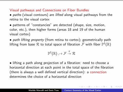
Visual pathways and Connections on Fiber Bundles• paths (visual contours) are lifted along visual pathways from theretina to the visual cortex
• patterns of “constancies” are detected (shape, size, motion,color, etc.), then higher forms (areas 18 and 19 of the humanvisual cortex)
• path lifting property (from retina to cortex); geometrically pathlifting from base R to total space of fibration F with fiber P1(R)
P1(R) ↪→ Fπ� R
• lifting a path along projection of a fibration: need to choose ahorizontal direction at each point in the total space of the fibration(there is always a well defined vertical direction): a connectiondetermines the choice of a horizontal direction
Matilde Marcolli and Doris Tsao Contact Geometry of the Visual Cortex

horizontal and vertical subspaces in the tangent space of a fibration
Matilde Marcolli and Doris Tsao Contact Geometry of the Visual Cortex
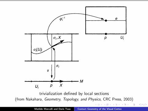
trivialization defined by local sections(from Nakahara, Geometry, Topology, and Physics, CRC Press, 2003)
Matilde Marcolli and Doris Tsao Contact Geometry of the Visual Cortex

path lifting to the visual cortex (Hoffman)
Matilde Marcolli and Doris Tsao Contact Geometry of the Visual Cortex

Connection 1-form and Contact Planes
• connections and 1-forms: view a connection as a splitting ofexact sequence
TP1 → TF π∗−→ TR
of tangent spaces of fibration: choice of horizontal direction ateach point; achieved by a 1-form α (scalar valued because circlebundle P1(R) ' S1) while vertical direction is V = ker(π∗)
• Geometric Model: orientation response fields (ORFs) are contactplanes ξ = ker(α) determined by the connection 1-form α thatperforms the path lifting from the retina to the visual cortex
Matilde Marcolli and Doris Tsao Contact Geometry of the Visual Cortex
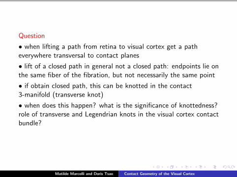
Question
• when lifting a path from retina to visual cortex get a patheverywhere transversal to contact planes
• lift of a closed path in general not a closed path: endpoints lie onthe same fiber of the fibration, but not necessarily the same point
• if obtain closed path, this can be knotted in the contact3-manifold (transverse knot)
• when does this happen? what is the significance of knottedness?role of transverse and Legendrian knots in the visual cortex contactbundle?
Matilde Marcolli and Doris Tsao Contact Geometry of the Visual Cortex
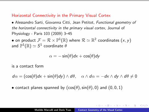
Horizontal Connectivity in the Primary Visual Cortex
• Alessandro Sarti, Giovanna Citti, Jean Petitot, Functional geometry of
the horizontal connectivity in the primary visual cortex, Journal of
Physiology - Paris 103 (2009) 3–45
• on product F = R× P1(R) where R ' R2 coordinates (x , y)and P1(R) ' S1 coordinate θ
α = − sin(θ)dx + cos(θ)dy
is a contact form
dα = (cos(θ)dx + sin(θ)dy) ∧ dθ, α ∧ dα = −dx ∧ dy ∧ dθ 6= 0
• contact planes spanned by (cos(θ), sin(θ), 0) and (0, 0, 1)
Matilde Marcolli and Doris Tsao Contact Geometry of the Visual Cortex
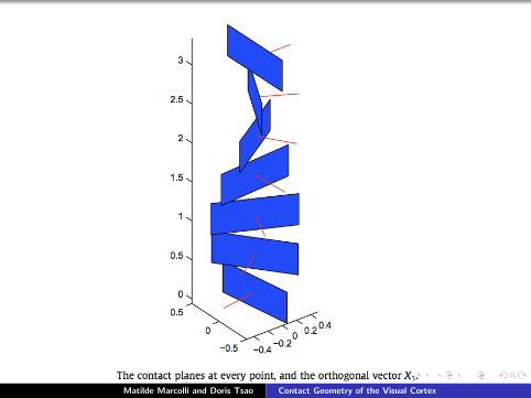
Matilde Marcolli and Doris Tsao Contact Geometry of the Visual Cortex
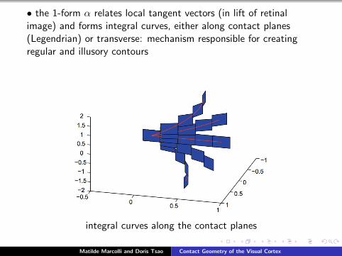
• the 1-form α relates local tangent vectors (in lift of retinalimage) and forms integral curves, either along contact planes(Legendrian) or transverse: mechanism responsible for creatingregular and illusory contours
integral curves along the contact planes
Matilde Marcolli and Doris Tsao Contact Geometry of the Visual Cortex

Scale Variable
• an additional scale variable σ ∈ R+: think of the visual fieldinformation recorded in the lift to the visual cortex not as a deltafunction but as a smeared distribution with Gaussian parameter σ(Gabor frames)
• when σ → 0 recover geometric picture described above withintegral curves
• geometric space X = R2 × S1 × R+, coordinates (x , y , θ, σ)
• 2-form on X : scale α 7→ σ−1α
ω = d(σ−1α) = σ−1dα + σ−2α ∧ dσ
symplectic ω ∧ ω = 2σ−3dα ∧ α ∧ dσ = 2σ−3dx ∧ dy ∧ dθ ∧ dσ
• not symplectically filling: blowing up at σ → 0, don’t have ω|ξ atboundary, but dα + α ∧ dσ would be
Matilde Marcolli and Doris Tsao Contact Geometry of the Visual Cortex

• ω = σ−1ω1 ∧ ω2 + σ−2ω3 ∧ ω4 with ωi 1-form dual to vectorfield Xi , corresponding vector fields
X1 = cos(θ)∂x + sin(θ)∂y , X2 = ∂θ,X3 = − sin(θ)∂x + cos(θ)∂y , X4 = ∂σ
• for small σ predominant X1X2 contact planes; for large σpredominant X3X4-planes
integral curves in the X1X2-planes and in the X3X4-planes
Matilde Marcolli and Doris Tsao Contact Geometry of the Visual Cortex
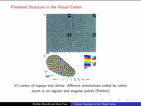
Pinwheel Structure in the Visual Cortex
V1 cortex of tupaya tree shrew: different orientations coded by colors
zoom in on regular and singular points (Petitot)
Matilde Marcolli and Doris Tsao Contact Geometry of the Visual Cortex
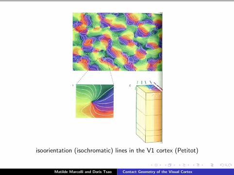
isoorientation (isochromatic) lines in the V1 cortex (Petitot)
Matilde Marcolli and Doris Tsao Contact Geometry of the Visual Cortex
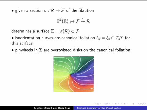
• given a section σ : R → F of the fibration
P1(R) ↪→ Fπ� R
determines a surface Σ = σ(R) ⊂ F• isoorientation curves are canonical foliation `x = ξx ∩ TxΣ forthis surface
• pinwheels in Σ are overtwisted disks on the canonical foliation
Matilde Marcolli and Doris Tsao Contact Geometry of the Visual Cortex
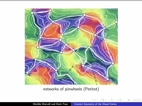
networks of pinwheels (Petitot)
Matilde Marcolli and Doris Tsao Contact Geometry of the Visual Cortex
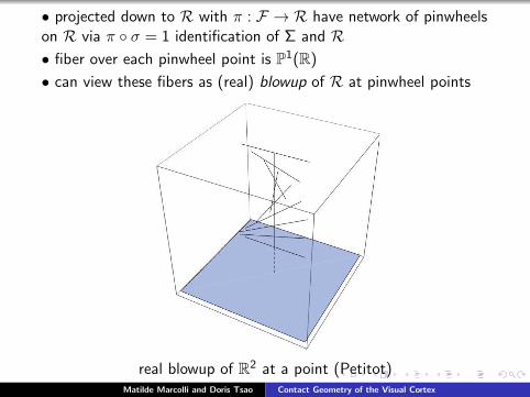
• projected down to R with π : F → R have network of pinwheelson R via π ◦ σ = 1 identification of Σ and R• fiber over each pinwheel point is P1(R)
• can view these fibers as (real) blowup of R at pinwheel points
real blowup of R2 at a point (Petitot)Matilde Marcolli and Doris Tsao Contact Geometry of the Visual Cortex

BlpA2 = {(x , y), [z : w ] | xz + yw = 0} ⊂ A2 × P1
BlpA2 = {(q, `) | p, q ∈ `}for p 6= q projection π1 : BlpA2 → A2, (q, `) 7→ q isomorphism,because unique line ` through p and q, but over p = q fiber is P1
set of all lines `
real blowup of R2 at a point (image by Charles Staats)
Matilde Marcolli and Doris Tsao Contact Geometry of the Visual Cortex

pinwheels in the base R and fibers (Petitot)
Matilde Marcolli and Doris Tsao Contact Geometry of the Visual Cortex
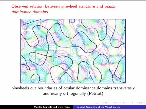
Observed relation between pinwheel structure and oculardominance domains
pinwheels cut boundaries of ocular dominance domains transverselyand nearly orthogonally (Petitot)
Matilde Marcolli and Doris Tsao Contact Geometry of the Visual Cortex