Embed Size (px)
Citation preview

Consumer Search with Observational Learning∗
Very Preliminary and Incomplete. Please Do Not Circulate.
Daniel Garcia† Sandro Shelegia‡
May 2, 2014
Abstract
This paper studies social learning in a search environment. We model consumers
who observe other consumers’ purchasing decisions before embarking on their own
search for the best-fitting product. This form of social learning has two distinct
effects on consumer search and firm pricing. First, consumers emulate others in
the sense that they always make the first visit to the firm where their predecessor
has purchased. Second, consumers free-ride on their predecessor’s information and
search less intensively than in the standard search model. Emulation encourages
price competition because firms fight for consumer visits, while free-riding has the
opposite effect due to reduced search. Both effects increase in the search cost, but
emulation is shown to dominate for most commonly used distributions of consumer
preferences, therefore prices (eventually) fall as search cost increases, and may even
go down to the marginal cost. We show that the results derived in a static duopoly
model remain valid with a large number of firms and can be extended to a dynamic
framework.
JEL Classification: D11, D83, L13
Keywords: Consumer Search; Observational Learning, Emulation
∗We thank Maarten Janssen for insightful comments on an earlier version. Garcia gratefully acknowl-edges financial support by the Hardegg Foundation. All errors are to be attributed to the authors only.†Department of Economics, University of Vienna. Email: [email protected]‡Department of Economics, University of Vienna. Email: [email protected]
1
1 Introduction
Observational learning has been the object of study of an increasingly large literature
in economics since the seminal contributions of Banerjee (1992) and Bikhchandani et al.
(1992). In the classical model, a sequence of individuals faces a simple decision prob-
lem under uncertainty and where each individual observes the history of decisions of her
predecessors. As argued by Banerjee (1992), this simple environment closely resembles
the problem faced by consumers in many markets, where previous customers’ choices
may be informative about the relative value of different products. Search markets, where
consumers have to actively engage in costly activities to gather information about dif-
ferent options available to them, seem to be prominent examples of such environments.
Intuitively, new consumers may free ride on the search effort of others and follow their
advice. Importantly, this would substantially change the elasticity of demand and, hence,
equilibrium prices. Thus, observational learning in search markets may have important
implications on search behavior and ultimately on prices.
To the best of our knowledge, no paper has studied this important issue. We attempt
to bridge this gap by analyzing a simple duopoly model of search with heterogenous
products in the spirit of Wolinsky (1986). In the model, a large number of consumers
derive utility from a given good, that comes in two varieties sold by two different firms.
Consumers are initially uninformed about their valuation for each variety or the price
charged by each firm, but learn them after engaging in costly sequential search. These
valuations are randomly drawn from some variety-specific distribution. Firms simultane-
ously choose prices so as to maximize expected profits taking the behavior of consumers
as given. To this fairly standard setup borrowed from Wolinsky (1986) and Anderson and
Renault (1999) (henceforth ARW ) we add observational learning by informing individual
consumers of the purchasing decision of their predecessor whose valuation is positively cor-
related with consumer’s own valuation. Importantly, consumers do not observe whether
their predecessors searched actively nor the price or utility derived. Thus, this is a model
of (limited) observational learning.
Strikingly, this change in the information structure of consumers radically changes
equilibrium outcomes. In the ARW model, consumers’ first visit is directed to each firm
with equal probability (which is indeed optimal since the resulting equilibrium prices are
equal). In our framework, because utilities are positively correlated, consumers decide to
search first the variety purchased by their predecessor. As consequence, the proportion of
first visits to a firm coincides (in the long-run) with her market share, and since consumers
are more likely to buy the variety they sample first, this leads to a social multiplier of
demand. To understand the effect of this change, we first assume that the correlation
between consumers’ valuation is positive but negligibly small, so that in a symmetric
equilibrium consumers learn nothing from their predecessors but still follow them for their
2

first visit (which is still optimal). We show that in the resulting equilibrium, prices are
lower than in the ARW model, and for all commonly used distributions prices decrease
in search cost once search cost is sufficiently large. The difference between our and
Wolinsky-Anderson-Renault model stems from the behavior of consumers who always
buy the variety they sample first (because their valuations for both products exceed their
reservation utility). In the ARW model, the firm who is visited by these consumers first is
effectively a monopolist and, thus, as the proportion of such consumers increase, as it does
when search cost rises, prices tend to increase. In our model, however, these consumers
are allocated according to the share of searchers who visit both stores. Since firms cannot
price-discriminate between the two groups, as the proportion of consumers who stop at
the first store increases, firms engage in increasingly fiercer competition for searchers who
determine market shares, leading to Bertrand-like competition and eventually to prices
that can be as low as the marginal cost.
We then introduce differences in the distributions of valuations of each variety. More
precisely, we assume that the valuations that consumers derive from the variety offered
by each firm are drawn from one of two distributions, and one of those distributions
(High) dominates the other (Low) in the First Order Stochastic sense. Assuming that
neither firms nor consumers observe which distribution realized, we can focus on the effect
of learning in consumer behavior and prices. Note that a previous purchase of a given
variety leads to an upwards update of its distribution of valuations and a downwards
update in the rival’s distribution. Hence, consumers are now willing to accept a lower
surplus from their first visit, thus reducing search effort. We term this the free-riding
effect of observational learning.
The effects on equilibrium prices are, however, not straightforward. On the one hand,
as explained above, less search leads to higher competition because the social multiplier
becomes more important. On the other hand, a price deviation triggers a change of beliefs
that may overcome this effect. If a firm deviates to a higher price, the proportion of sales
in each demand state changes, thus changing the beliefs that incoming consumers have.
Since the elasticity of demand is lower for the firm with a higher distribution of valuations,
consumers become more pessimistic about its rival’s distribution the higher is the price
of the store they visit. Hence, the surplus (net of the price) they demand for buying
right-away decreases in the price, reducing the elasticity and increasing prices. We show
that for some distributions, such as uniform and normal, the second effect is stronger for
relatively small search costs while eventually the second effect dominates and prices may
be lower than in the model without learning.
We are able to show that, just as in the model with emulation but no learning, in the
model with learning, under a regularity condition, prices eventually decline in search cost
and fall all the way down to marginal cost. The issue hinges on whether the likelihood
ratio is sufficiently informative in the extreme case where almost no consumers search
3

except those with the lowest valuations for one of the products. We are able to show that
distributions with finite lower bound always satisfy the condition, and so ore prediction
on the relationship between search cost and equilibrium prices is rather robust.
In the reminder of the paper we consider extensions to oligopoly and dynamic pricing.
First we study the effects of competition on equilibrium prices in the model without
learning. We show that prices decrease in search cost and converge to marginal costs
as the proportion of movers vanish, for any number of firms. We further show that
prices decrease in the number of firms for any search cost. Of special interest is the limit
price when the number of firms grows large. In this case, whether there is correlation
across individuals or not, there is nothing to be learnt about rival firms’ qualities from
the realization of sampled varieties. Armstrong and Chen (2009) shows that, as long as
it is exogenous, the order of visits does not change prices in the ARW model since the
elasticity of demand is the same for all firms. In our model, however, prices are lower than
in the ARW model and have a U-shape relationship with search costs. If search costs
are very low and there are many firms, Bertrand competition for buyers obtains. On the
other hand, if search costs are very high, we know that firms fiercely compete for first
visits and prices also converge to marginal costs. For intermediate search costs, however,
firms charge positive prices.
Regarding dynamic pricing we show that if firms can adjust prices after the introduc-
tory period, and that in subsequent periods consumers make first visits proportional to
first-period market shares, prices are further reduced in the introductory period with ob-
servational learning, and then go up to the levels of the ARW model. Thus observational
learning mechanism is complementary to the dynamic market share buildup mechanism
and together they lead to a very low introductory prices and then price hikes.
Literature Review
Our model of observational learning is inspired by recent evidence in economics and mar-
keting. Mobius et al. (2005) present results of a field experiment designed to understand
individual demand for different products for which individuals receive information. They
show that those subjects who are connected through social links to others who are in-
formed about a particular good, value the goods more. Importantly, they find that this
effect is stronger for gadgets than for services, which are more likely to be subject to
direct observation. In another field experiment, Cai et al. (2009) show that restaurant-
goers are more likely to order those goods that are presented to them as more popular.
Finally, Moretti (2011) analyzes the movie market where an unexpected increase in the
first-week’s box office has a persistent a significant effect in future attendance.
Two recent papers have analyzed consumer search with observational learning, but
both assume that prices are fixed exogenously. Kircher and Postlewaite (2008) study
4

consumers who differ in their willingness to search and firms differ in quality. Although
prices are fixed, firms may decide to offer a valuable service to any consumer who visit
their store. They show that equilibria may arise where high-quality firms offer service to
those consumers who search more actively and those who search less actively follow their
advice. Hendricks et al. (2012) presents a model of observational learning with multiple
types in the spirit of Smith and Sørensen (2000) where each consumer has to decide
between acquiring a costly signal about quality of a single good, buying it right-away or
not buying. The model is cast in a more traditional herding framework where consumer
receive a signal before deciding whether to engage in costly search. They focus on the
long-run dynamics of sales for high and low quality products and the possibility of bad
herds arising. Our model lacks pre-search information, therefore we cannot study bad
herds, but instead focus on pricing.
In the consumer search literature with price competition, closest papers to ours are
Armstrong et al. (2009) and Armstrong and Zhou (2011), who present a model of promi-
nence in consumer search where one firm is sampled first by all customers. In Armstrong
et al. (2009) a given firm is made prominent exogenously. In the resulting equilibrium, the
prominent firm charges a lower price than her rivals because her share of returning cus-
tomers (who are typically less responsive to prices) is lower. One may view our framework
as that of endogenous prominence, where share of first visits depends on price. Armstrong
et al. (2009) show that as the number of firms grows, (exogenous) prominence becomes
irrelevant while in our model, competition becomes even fiercer and prices decrease in the
number of firms. Armstrong and Zhou (2011) study several different models that endog-
enize firm’s prominence. One such model is based on observable price competition where
consumers rationally search the lowest-pricing firm first. Because demand is discontinu-
ous in prices, the resulting equilibrium involves mixed strategies and has a property that
higher search cost leads to (stochastically) lower prices. One may view observability of
prices as an extreme example of observational learning where consumers observe market
shares, and thus prices. We show that imprecise information about prices results in a
pure strategy equilibrium featuring inverse relationship between search cost and prices.
Another closely related model can be found in Haan and Moraga-Gonzalez (2011), where
prominence depends on advertising efforts and firm profits may decrease in search cost
(although prices increase and consumer surplus decreases).
Our paper is also related to the literature that studies effects of social learning on
monopoly pricing. Campbell (2013) and Chuhay (2010) analyze the impact of word-of-
mouth communication on the monopoly price and product design. Perhaps closest to our
work are two contributions by Bose et al. (2006) and Bose et al. (2008) who study dynamic
interaction between a monopolist and a sequence of consumers with common valuation
who observe each other purchasing decisions. While most of this literature has studies
monopoly, an exception is Kovac and Schmidt (2014) who study a dynamic market where
5

two firms offer a homogenous product and consumers learn prices from others. Since
our focus is on competition and we abstract from dynamic issues1, we view our work as
complementary to theirs.
Finally, a number of papers have studied the relation between current market shares
and future demand. Becker (1991) directly introduces aggregate demand into the in-
dividual utility function. Caminal and Vives (1996) studies a dynamic signaling game
where new cohorts of consumers observe past market shares of an experience good, but
not prices and try to infer quality from this information. Firms use prices to manipulate
market shares to attract consumers. While their setting is different in that consumers do
not search, we also find that firms use prices to attract consumers, but here consumers
free-ride on their predecessors’ efforts and due to search cost, herds form, while in Caminal
and Vives these effects are mute.
The next section introduces the general model with observational learning with cor-
related preferences and endogenous prices. Section 3 solve the model in the special case
of no correlation between preferences of consumers. Section 4 studies the model with
correlated preferences and establishes comparative statics results including with respect
to the number of firms. Section 5 introduces an extension to dynamic pricing and Section
6 concludes.
2 Model
Consider a market populated by a large number of consumers i = 1, 2, ..N , interested in
purchasing a single unit of a differentiated good that comes in two varieties, each sold by
one firm, 1 and 2. Consumers are initially uncertain about their valuation of each firm’s
product, but may acquire this information through sequential search. We assume that
the first visit is free but the second has a cost of c in utility units and all consumers can
recall their previously sampled varieties at no additional cost. Following Anderson and
Renault (1999) we make the simplifying assumption that all consumers will buy one of
the two varieties.2
We describe now the demographics of the model. In every period, a cohort of con-
sumers arrive to the market. Every consumer makes all his decisions in that one period.
Let 1 ≤ ti ≤ T be the period in which consumer i arrives. The utility that every consumer
i derives from variety j depends on his type k ∈ {1, 2, .., K}, and in each cohort there is
a single individual of each type, so that there are N = K · T consumers. Consumers do
not know ti and hold a common prior ν(t) over it. We introduce observational learning
by informing every consumer arriving in a cohort t > 1 of the purchasing decision of the
previous consumer of his type. Importantly, they do not observe the information that has
1See Section 42This amounts to assuming that their outside option is sufficiently bad.
6
led to the purchase or whether their predecessor sampled more than one variety.
We introduce correlation between preferences of individuals of a given type in the
following fashion. All consumers of a type draw their valuations for each firm’s product
from one of two potential distributions, a High distribution (denoted by GH(u)) and a
Low distribution (GL(u)). Both distributions are equally likely to realize for each type,
and these realizations are independent across types and firms. We assume that both
distributions have the same (possibly infinite) support [u, u] and that GH First Order
Stochastically Dominates (FOSD) GL. Let gH and gL be the corresponding densities.
As is usual in the economics literature, we assume that the Monotone Likelihood Ratio
property holds so that gH(x)gL(x)
is an increasing function of x. Let λ(u) = gH(u)gH(u)+gL(u)
be the
conditional probability of H given u. Let G(u) = 12GH(u) + 1
2GL(u) be the unconditional
distribution of valuations of a random consumer. We shall assume that G(u) is log-
concave.3 Finally let (S1, S2)k ∈ {H,L}2 be the realized state for a given type. To
summarize, all consumers of the same type draw their utility for a firm from the same
distribution. E.g. consumers of type k may draw their utility from distribution H for
firm 1 and L for firm 2. Even though consumers cannot know the utility of the consumer
they observed, the fact that that consumer buys from a firm is informative about which
state (S1, S2)k has realized.
In order to disentangle changes in information from changes in the distribution of
valuations, it is convenient to define two auxiliary distributions G1(u) and G2(u) such
that GH(u) = (1 − r)G(u) + rG1(u) while GL(u) = (1 − r)G(u) + rGL(u) and such
that G(u) = 12G1(u) + 1
2G1(u), where r ∈ [0, 1] measures the degree of correlation across
consumers of a given type. This specification guarantees that for any r the unconditional
distribution (without knowing state S) for a firm is G(u), while r controls how close GL
is to G1 and GH is to G2. If r = 0 valuations are independent, and drawn from G(u),
while for r > 0 valuations of any two members of the same type are positively correlated.
Conveniently, for every r the unconditional distribution of valuations remains constant but
the amount of information contained in the purchasing decision of a predecessor may vary
significantly (as allowed by the disparity between G1 and G2). Thus r proxies correlation
of valuations among members of a type.
On the supply side, there are two firms supplying any quantity of their variety at a
constant unit cost normalized to zero. Importantly, firms commit to serve all incoming
customers at a single price pj set simultaneously before the state of the market is realized in
order to maximize expected profits. We shall devote most of our attention to a symmetric,
pure-strategy equilibrium where both firms charge the same price p∗.
3Log-concavity of GH and GL does not guarantee Log-concavity of G.
7

2.1 Consumer Behavior
Consumers in the first cohort, lacking any information to discriminate firms, make their
first visit randomly and buy there if and only if ui − pi > w − p∗, where w solves∫ u
w
(u− w)g(u)du = c, (1)
where g(u) = gH(u)+gL(u)2
and is the density of G(u). w is the familiar reservation utility
from Wolinsky (1986). It is found by equalizing expected benefit from search (with free
recall) to the search cost. Unsurprisingly, the first consumer of any type is no different in
our model as compared to the ARW model.
As is well known, in ARW there is no search for c >∫ uuug(u)du, adn in the version of
the model where the outside option is infinitely bad, prices are infinitely large. To avoid
this, henceforth we assume
Assumption 1. The search cost satisfies c <∫ uuug(u)du ≡ c.
All remaining consumers observe a predecessor buying from firm j and expect the
same price p∗ in both stores before embarking on their first search. Since valuations are
positively correlated, the expected surplus from firm visiting firmj is (weakly) larger than
that of firm −j and so the consumer should visit that store. Upon visit consumer learns
his utility realization for good j, uij and the price that the firm j charges. Consumer will
search if and only if uij − pj < w(pj)− p∗, where w(pj) solves∫ u
w−pj+p∗(u− w + pj − p∗)(q(w; pj)gH(u) + (1− q(w; pj))gL(u))du = c (2)
where q(u; p) is the (posterior) probability that at the other store the valuations are drawn
from the high distribution. This probability will, in general, depend on the valuation
drawn from firm j (because preferences are correlated) and the price of firm j because it
affects the probability consumers buy at that firm, and thus conditional distribution of
the other store. In principle, q(u; p) is a very complicated object, since each consumer
may infer from u not only how likely it is that a given distribution realized but also his
cohort (which is potentially informative about the informational content of the purchasing
decision of the predecessor). In particular, the probability that a consumer arriving in
cohort t buys from firm 1 if the state is (SS ′) ∈ {H,L}2 is
xtSS′(p1, p2) = xt−1SS′(p1, p2)(1−GS(w(p1))) + (1− xt−1
SS′(p1, p2))GS′(w(p2))(1−GS(w(p1)))
+
∫ w(p1)−p1+p2
u
GS′(u− p1 + p2)gS(u)du
which increases in xt−1SS′ , leading to a link between past and current market shares. It
8

is straightforward to see that this mapping has a fixed point where market shares are
stationary (xSS′(p1, p2)). In Appendix 1 we show that, provided that the number of con-
sumers of each type is sufficiently large, consumers’ optimal search strategy is arbitrarily
close to the one computed for a stationary market share distribution. In this case, drop-
ping the time subscript, we can write a firm’s market share in state SS ′ when it charges
p while the other firm charges the equilibrium price as
xSS′(p, p∗) = xSS′(p, p
∗)(1−GS(w(p))) + (1− xSS′(p, p∗))GS′(w(p))(1−GS(w(p)))
+
∫ w(p)−p+p∗
u
GS′(u− p+ p∗)gS(u)du.
We can solve for xSS′(p, p∗) from the above
xSS′(p, p∗) =
∫−p∗+p+w∗−∞ gS(u)GS′ (p
∗−p+u) du+(1−GS(−p∗+p+w∗))GS′ (w∗)∫−p∗+p+w∗
−∞ gS(u)GS′ (p∗−p+u) du−
∫ w(p)−∞ gS(u)GS′ (p
∗−p+u) du+(1−GS(−p∗+p+w∗))GS′ (w∗)+GS(w(p))
.(3)
For stationary market shares, q(u; p) satisfies
q∗(u; p) =xHH(p)λ(u) + xLH(p)(1− λ(u))
(xHH(p) + xHL(p))λ(u) + (xLH(p) + xLL(p))(1− λ(u))(4)
The above formula uses market shares in every state and weights the conditional proba-
bility of H given u by these market shares. As expected, if in all states both firms have
equal market share (xSS′ = 1/2), which given our assumption about GH and GL imply
GL = GH , the first visit is not informative and q∗(u; p) = 1/2. Notice that q∗(u; p) is in-
creasing in u because λ is an increasing function and the market shares satisfy xHH ≥ xLH
and xHL ≥ xLL. Intuitively, a higher u leads the consumer to update upwards the prob-
ability he attaches to the current firm having a high distribution (S = H). Importantly,
this also increases the belief he holds about the other firm’s distribution, since it reduces
the informativeness of the predecessor’s purchase at this firm regarding the other firm’s
distribution.
This completes the characterization of the consumer search rule. In particular, w(p)
is implicitly defined in (2) where q(u; p) is given by (4) where xSS′ is defined in (3).
In the reminder of the paper we will use stationary market share distributions. One
may think of a reduced-form model where consumers observed a predecessor, proportion
of first visits matches firm’s market share, and search and firm strategies are consistent
with the above.
2.2 Equilibrium Conditions
In a symmetric equilibrium, prices are equal and, thus, do not affect search behavior. The
consumers’ search rule can be rewritten as
9
∫ u
w
(u− w)(q(w)gH(u) + (1− q(w))gL(u))du = c (5)
where q(w) = q(w; p∗) is the equilibrium probability that the rival firm has the High
distribution given the reservation utility. Notice that q(u) ≤ q(u) ≤ 12
since observing a
previous consumer buying in a store is bad news about the prospects in the rival store.
This effect is only fully mitigated if the consumer learns that the current firm offers high
valuations, in which case it learns nothing about his prospects in the rival firm. Hence,
we have the following trivial observation.
Proposition 1. Fix c > 0, in a unique symmetric equilibrium, w < w∗, and, hence,
consumers free-ride on others’ effort.
Firms’ profits depend on the search rule used by consumers both on and off-the-
equilibrium path. In particular, let w′(p) be the implicit derivative of the search cutoff
with respect to p. In the ARW model model without learning, w′(p) = 1 so that an
increase in price is compensated with a higher required utility. This is no longer the case
with observational learning. Consumers visiting a firm with a different price adjust their
beliefs about the distribution of valuations in the rival firm, while keeping their beliefs
about its price constant.4 In particular, the higher the price, the less likely it is that a
consumer ends up in that firm if its rival has a High realization of valuations. Thus, in
general, w′(p) < 1. Given this search behavior, consumers are split into four groups in the
(u1, u2) space (plot). As is standard in Wolinsky-type models, those whose valuation for
both varieties is lower than the reservation utility w search independently of the variety
they sample first and then buy from the highest-surplus offering firm. Those whose utility
profile satisfies uj < w < uk only search if they visit firm j and always buy from k. Finally,
those whose valuations are higher than their reservation utility buy from the firm they
visit first. This group has low-demand elasticity and is typically assigned randomly across
firms. In our model, these consumers are assigned to each firm with probabilities equal
to market shares and, thus, become quite elastic. We term this the emulation effect of
observational learning.
Expected demand for a firm that charges p while its competitor charges p∗ and con-
sumers use reservation utility function w(p) is the average of demands over all possible
states. Because states between firms are independent, and equally likely, the demand is
given by:
x(p, p∗) =1
4
∑SS′
xSS′(p, p∗). (6)
Here x(p, p∗) implicitly depends on w(p) and thus on consumer search rule.
4The assumption of passive beliefs is common in the literature. For a discussion see Janssen andShelegia (2014)
10

In equilibrium, symmetric equilibrium price satisfies the following condition
∑SS′
xSS′(p∗, p∗) + p∗
∑SS′
∂xSS′(p, p∗)
∂p= 0
and further∑
SS′ xSS′(p∗, p∗) = 1
2by symmetry. So the equilibrium pricing rule simplifies
to1
2+ p∗
∑SS′
∂xSS′(p1, p∗)
∂p1
= 0 (7)
Equations for xSS′ are non-trivial and depend on a complex way on the search rule
consumers use. Because of this, while we derive some results for any G and r > 0, before
proceeding to analyzing the general case we turn to the special case where r = 0.
3 Emulating Consumers
To better understand these two effects, we start by isolating emulation from free-riding.
We do so by assuming that r → 0 so that valuations across consumers are nearly in-
dependent, while consumers still follow others’ purchasing decisions for their first visits.
This is the limit case of the general model when distributions become increasingly similar,
and since the model is ex-ante symmetric, making the first visit to the firm where the
predecessor has purchased remains optimal (including when r = 0). More generally, one
can view this model as a behavioral modification of Anderson and Renault (1999) where
consumers’ first visits are allocated according to market shares rather than randomly.
While the modification is rather small, it has dramatic effect on prices.
Because the visit of the predecessor contains no information, the reservation utility is
computed as in the ARW model and is given by (1). As for the firms, let x denote market
share of firm 1. Because first visits also follow purchases, the share of firm 1’s first visits
is also x. Thus its demand can be written as
x(p1, p∗) = x(p1, p
∗)(1−G(w + p1 − p∗)) + (1− x(p1, p∗))G(w)(1−G(w + p1 − p∗))
+
∫ w+p1−p∗
u
G(u− p1 + p∗)g(u)du
From the above, it is straightforward to solve for x(p1, p∗) and find firm 1’s pricing
equation.
Proposition 2. Suppose r = 0. In a symmetric equilibrium with emulating consumers,
the reservation utility is computed as in (5) and the price is
p∗ =(2−G(w))G(w)
2∫ wug2(u)du+ (1−G(w))g(w)
(8)
11

while in the ARW model
p =1
2∫ wug2(u)du+ (1−G(w))g(w)
(9)
Thus, p∗ ≤ p, with a strict inequality for w∗ < u.
The intuition for this result is rather simple. In the ARW model, price competition
is restricted to the small subset of consumers whose valuations for both firms are close
and lower than the reservation utility. In the model with observational learning, those
consumers whose valuation for both varieties is larger than the reservation utility become
sensitive to price changes because they follow the lead of those with relatively low valua-
tions. This is the social multiplier effect on demand. As the proportion of consumers who
do not search beyond the first firm grows, price competition for searching consumers who
bring all others to the store intensifies leading to lower prices. Recall that c =∫ uuug(u)du
is the average utility at a given store. Using the argument above, we can state:
Proposition 3. For any log-concave G with bounded support, for any limc→c p = 0. Also,
if G has unbounded support but limu→uG(u)/g(u) = 0, then limc→∞ p = 0.
The first part of the proposition has been explained. The second part puts a restriction
on the ratio of the cumulative to the density at the lower bound that is satisfied by all
distributions whose support is bounded below as well as for most log-concave distributions
whose support is unbounded (e.g. Normal). This condition is not satisfied for the Logistic
distribution, but it can also be readily verified that prices decrease in search costs for this
distribution too.
4 Equilibrium with Learning
The effects of learning on prices is ex-ante ambiguous because learning adds two competing
effects. First, as highlighted by Proposition 1, for a given c and a symmetric price p∗, w
is lower the bigger the difference between distributions. Consumers are then willing to
accept lower surplus the higher the price (w′(p) < 1), which pushes prices upwards. On
the other hand, in the presence of emulation, lower w may lead to lower prices through
fiercer competition for increasingly rare searchers. This effects can be seen in pictures...
Notice that, eventually, free-riding joins forces with emulation and prices decrease
faster and converge to marginal cost for lower search costs than without learning. In
particular, the maximum search costs at which a pure-strategy equilibrium exists equals
the expected valuation of GL. This is because, in the example, the likelihood ratio grows
unboundedly at the lower bound. Hence, a consumer who arrives at a store offering
sufficiently low utility is almost sure that the current firm’s distribution of valuations is
12

Low, which implies that with arbitrarily high probability the rival offers Low valuations
too, for otherwise the probability that my predecessor ended up here is negligible. To see
this, notice that
limc→c
xSS′(p, p∗) =
GS′(w)
GS′(w) +GS(w(p))(10)
If λ(u) = 1, xL,H(p∗, p∗) = 0 and thus, q(u) = 0. In such a case, search is unattractive
and the consumer stays. Define cL =∫ uuugL(u)du. Since prices approach marginal costs
as the share of movers vanishes, we have the following counterpart of Proposition 3:
Proposition 4. Suppose G has a finite support. As c→ cL, we have p→ 0.
Prices converge to zero as the search cost converges to the expected valuation of GL.
The following Corollary suggests that learning itself may decrease prices by letting the
ex-ante distribution of valuations constant. Let p(r) be the price if the distribution is
governed by r ∈ [0, 1] and recall that higher r correspond to higher correlation and,
therefore, higher informativeness of the purchasing decision of a predecessor. We have
the following Corollary
Corollary 1. Take a distribution G. For c ∈ (cL, c), p(1) = 0 < p(0).
That is, as the informativeness of the purchasing decision increases, the equilibrium
price elasticity increases and, thus, prices decrease. This is because those consumers
whose valuation for the variety they sample first is low become increasingly pessimistic
about their prospects in the other store the higher is the correlation across consumers,
and, therefore, the less inclined they are to search.
The following figures illustrate our results for a uniform distribution G on [0, 1]. In
this example G1 is a triangular distribution on [0, 1] with mode 0 while G2 is a triangular
distribution on [0, 1] with model 1. As required, the mixture of the two is uniform on
[0, 1], GH FOSD GL and the likelihood ration is monotone for any r > 0.
Figures 1 and 2 show prices and reservation utilities in various models.
As expected, prices are always lower in the model with pure emulation (black) than
in the ARW model. As predicted by theory, in ARW model price is increasing in s and
reaches 1 at c = 1/2. This is where even a consumer who draws 0 at the first store refuses
to search further (after this, prices are infinite becuase outside option is −∞). In our
model with learning (r = 1), as predicted by Proposition 4, because u = 0 > −∞, price
is zero at c = 1/3, which is the average of G1. In our model without learning (r = 0),
price converges to zero at c = 1/2, as implied by Corollary 2. Intuition for both is simple.
When c = 1/3 in the model with learning, a consumer who is sure that utilities from the
other store are drawn from GL will not search. But this is what happens in equilibrium
when a consumer draws utility close to u - she reasons that because distribution in the
current firm is almost surely GL, the fact that she came here indicates that in the other
13
p
r=
1
ARW
r = 0
c0.1 0.2 0.3 0.4 0.5
0.2
0.4
0.6
0.8
1.0
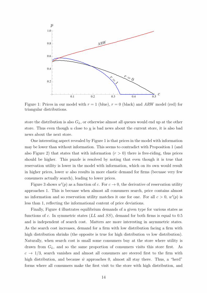
Figure 1: Prices in our model with r = 1 (blue), r = 0 (black) and ARW model (red) fortriangular distributions.
store the distribution is also GL, or otherwise almost all queues would end up at the other
store. Thus even though u close to u is bad news about the current store, it is also bad
news about the next store.
One interesting aspect revealed by Figure 1 is that prices in the model with information
may be lower than without information. This seems to contradict with Proposition 1 (and
also Figure 2) that states that with information (r > 0) there is free-riding, thus prices
should be higher. This puzzle is resolved by noting that even though it is true that
reservation utility is lower in the model with information, which on its own would result
in higher prices, lower w also results in more elastic demand for firms (becuase very few
consumers actually search), leading to lower prices.
Figure 3 shows w′(p) as a function of c. For c→ 0, the derivative of reservation utility
approaches 1. This is becuase when almost all consumers search, price contains almost
no information and so reservation utility matches it one for one. For all c > 0, w′(p) is
less than 1, reflecting the informational content of price deviations.
Finally, Figure 4 illustrates equilibrium demands of a given type for various states as
functions of c. In symmetric states (LL and SS), demand for both firms is equal to 0.5
and is independent of search cost. Matters are more interesting in asymmetric states.
As the search cost increases, demand for a firm with low distribution facing a firm with
high distribution shrinks (the opposite is true for high distribution vs low distribution).
Naturally, when search cost is small some consumers buy at the store where utility is
drawn from GL, and so the same proportion of consumers visits this store first. As
c → 1/3, search vanishes and almost all consumers are steered first to the firm with
high distribution, and because w approaches 0, almost all stay there. Thus, a “herd”
forms where all consumers make the first visit to the store with high distribution, and
14

w
r =1
ARWand r = 0
c0.1 0.2 0.3 0.4 0.5
0.2
0.4
0.6
0.8
Figure 2: Reservation utilities in our model with r = 1 (blue) and our model with r = 0and also ARW model (red) for triangular distributions.
then correctly avoid searching further.5 The interesting aspect of such optimal collective
behavior is that it coincides with zero prices. Note though that prices are zero not because
of optimal collective behavior in equilibrium, but rather for the opposite reason out of
equilibrium. Namely, if a firm were to deviate and charge a higher price, even though for
a quarter of types the state is HL, almost no consumers of these types would visit it. This
means that upon price deviations “bad herds” form where small price differences result in
quarter of consumer incorrectly visiting a firm with worse distribution and slightly better
price.
4.1 The Effects of Competition
We have assumed throughout that there are only two firms in the market. This assumption
ensures that both decisions and information sets are binary and renders the analysis of
consumer learning and behavior tractable. As the number of firms increases, the number
of states increases exponentially and so do the complexity of the information structure.
Thus, to analyze the effects of competition we go back to the simple model of consumers’
emulation where the learning channel is muted (i.e. r = 0). Notice, however, that as
the number of firms becomes larger, and learning becomes more complex, the amount
of information about other firms’ distribution contained in the purchasing decision of a
predecessor also decays exponentially. Intuitively, as the number of firms grows large, the
market share of a given firm is, approximately, independent of the realization of the state
in any other firm (mean-field approximation). Thus, while a purchasing decision by a
5The word “herd” here is used in contrast to the economics literature. In our model consumers donot possess pre-search information, and have to obtain it actively, thus herds in traditional sense cannotarise.
15

w0(p)
c0.1 0.2 0.3 0.4 0.5
0.88
0.90
0.92
0.94
0.96
Figure 3: Derivative of reservation utility with respect to p in our model for r = 1 andtriangular distributions.
predecessor remains informative about the distribution of valuations for the variety sold
in the current firm, it is irrelevant in determining the distribution of valuations for any
other variety.
Hence, assume that r = 0 and let n be the number of firms in the market. The
stationary market share of a given firm choosing a price p if all its rivals choose p∗ is
x(p, p∗) = x(p, p∗)(1−G(w − p∗ + p)) +1− x(p, p∗)
n− 1
n−1∑j=1
G(w)j(1−G(w − p∗ + p))
+
∫ w−p∗+p
u
G(u− p+ p∗)n−1g(u− p+ p∗)du.
Notice that market shares only determine the number of first visits to each firm, but not
the subsequent searches. Let p∗n be the price in a symmetric equilibrium with n firms.
For an arbitrary distribution G, we have
p∗n =nG(w)−G(w)n
n−1
g(w)(∑n−2
i=0 G(w)i+(n−1)G(w)n−1)−(n−1)n∫ wu G(u)n−2g(u)2 du
. (11)
Recall that w is still defined by (5). This can be contrasted with the equilibrium price in
the ARW model given by
pn = 1
g(w)(∑n−2
i=0 G(w)i−(n−1)G(w)n−1)+(n−1)n∫ wu G(u)n−2g(u)2 du
. (12)
Proposition 5. Assume r = 0. For every n and bounded G, the price with emulating
16

xHL(p⇤ , p
⇤)
xLH (p⇤, p⇤)
x
xHH(p⇤, p⇤) = xLL(p⇤, p⇤)
c0.1 0.2 0.3 0.4 0.5
0.2
0.4
0.6
0.8
1.0
Figure 4: Equilibrium demand of a given type for various states for triangular distribu-tions.
consumers is lower than the price in the ARW model and goes to zero with c. Further, pn
but also p∗n/pn decreases in n.
As with the ARW model prices go to zero with n in our model. Important distinction
is that as the number of firms grows, the relative gap between prices in our and ARW
model also grows, thus competition compounds the emulation effect.
The comparison becomes more clear when we take the limit as the number of firms
grows. In this case, thee share of returning customers vanishes and the price converges to
p∗∞ =(1−G(w))G(w)
g(w)(13)
so that limc→0 p∗∞ = limc→c p
∗∞ = 0. On the other hand, as shown in Anderson and
Renault (1999), the price in the ARW model (eq. 12) with an infinite number of firms
coincides the classical Perloff-Salop formula
p∞ =1−G(w)
g(w). (14)
Armstrong et al. (2009) shows that this price is independent of the way consumers
decide their search paths, as long as this order is exogenous. This shows that the effect of
prominence is qualitatively different from the effect of emulation, particularly when the
number of firms is large.
The next figure illustrates equilibrium prices for different n. As shown in Proposition
5, prices decrease in n.
17

0.1 0.2 0.3 0.4 0.5
0.2
0.4
0.6
0.8
1.0p
c
Figure 5: Equilibrium prices as function of search cost for n = 2 (purple), n = 4 (red)and n =∞ (blue) for our model (solid) and ARW (dashed).
5 Dynamics and Lock-in Effects
In this Section we explore the connection between our model and the Switching Cost
literature and, in so doing, introduce dynamic considerations. We consider the following
extension of the Benchmark model. The economy has two dates τ = 1, 2. In τ = 1 the
market structure is as presented above. Firms set prices for the first date and consumers
arrive in different cohorts and observe their predecessors’ purchasing decision. In τ = 2,
firms observe their sales and simultaneously choose prices for the second date. In order
to introduce a simple dynamic link we assume that consumers visit first the store they
purchased from in the first period but their utilities are drawn anew. As in the standard
switching cost model, the market in the first date is more competitive than in the second.
In this case, the difference in competition comes from the observational learning that does
not occur in the second Again, for simplicity, we assume that r = 0, so that no learning
about demand occurs in equilibrium. Further, we follow Armstrong et al. (2009) and
assume that valuations are uniformly distributed in [0, 1].
In the second periods, firms choose prices to maximize expected profits given their
number of first visit. In particular, given a share of first-date market, her second-date
market share is
x2(p, p2(x1)) = x1(1− (w − p+ p2(x1))) +
(1− x1)(w − p2(x1) + p1(x1))(1− (w − p+ p2(x1))) +∫ w−p+p2(x1)
u(u− w + p− p2(x1))du
Let ∆∗ = p1(x1)− p2(x1) be the expected difference in prices in the second period given
18

some market shares and let ∆ = p− p2(x1) be the realized difference. We have
x2(∆) = x1(1− (w −∆)) + (1− x1)(w −∆∗)(1− (w −∆)) +
∫ w−∆
u
(u− w + ∆)du
From Haan and Moraga-Gonzalez (2011) we know that ∆(x1) is increasing in x1 and
∆∗(12) = 0. If a symmetric equilibrium exists ∆∗ = 0 and p2(x∗1) = p2(1
2) = p. Now, let
π(x1) be the expected profit in the second date given market share x1. π(x1) is clearly
increasing in x1. Firm 1 solves then
maxp1
p1x1(p1, p∗) + π(x1(p1, p
∗)) (15)
Clearly p∗1 ≤ p∗ and in any symmetric p2(x∗1) > p∗1 so that prices increase over time.
6 Nature of observational learning
In our model consumers observe the purchasing decision of a single predecessor. While this
assumption is rather crude, it is perhaps more plausible than assuming that consumers
observe the whole sequence of purchasing decisions or the true market shares. In any case,
this assumption greatly simplifies the analysis since the number of possible information
sets a given consumer may end up in grows exponentially in the number of predecessors.
More importantly, in our model all consumers have the same reservation utility strategy.
This would not be the case if they observe a larger set of consumers. On the other hand,
if consumers observed market shares without noise, the equilibrium would converge to
the mixed-strategy pricing equilibrium presented in Armstrong and Zhou (2011) for the
case in which consumers observe prices. The reason for this is that even a small deviation
in price would result in all consumers first visiting the deviating firm, thus profit would
jump up discretely. This is the familiar Bertrand pressure on prices. But prices cannot be
zero becuase for relatively small search cost a firm can still earn profit even if it is visited
last. Therefore, there has to be a mixed strategy equilibrium.6
This shows that when consumers posses a lot of information about their predecessors’
purchases, equilibrium results in mixed strategies. We analyze the other extreme where
consumers have very limited information. What happens between these two extremes is
extremely hard to analyze, but we believe that for relatively limited observational learning
equilibrium is qualitatively similar to ours, until when a lot of learning results in mixed
strategies.
6This is in contrast to our results (Propositions 3 and 4) that say that prices go down to zero.Theresearch costs are so high that almost no one searches beyond the first firm, thus not matching the otherfirm’s low price results in zero profits.
19

7 Discussion
Our aim in this paper was to introduce simple observational learning into a standard
consumer search model with horizontally differentiated products. We did so and showed
that consumer search models change qualitatively with such learning.
To achieve this goal, we have made several important assumptions that can be relaxed
and or modified in future work. First, we followed Anderson and Renault (1999) in
assuming that all consumers buy. This assumption greatly increases the tractability of
the search model and simplifies learning across individuals. In its defense, it should be
noted that an extensive margin of demand should push prices downwards. Since our
main results concern surprisingly low prices, an active extensive margin would reinforce
these results. Moreover, it allows us to concentrate on the business-stealing effect of
information, since the amount of purchases is kept constant.
Second, we have introduced correlation across consumers’ valuations in the simplest
feasible way. If we went one step further in the direction of simplicity, and assumed that
all consumers of the same type have the same utility, the equilibrium search rule would not
have standard reservation utility property. This is because, in a putative cutoff-strategy
equilibrium, the purchasing decision of a predecessor is more informative for utilities just
below the cutoff and so search is less valuable there. Therefore, consumers would want to
stop for utilities below the cutoff. As a result, the equilibrium would have to feature an
interval of utilities where probability of searching further transitions smoothly from one
to zero. Although very interesting, this search rule renders the full model less tractable.
Moving in the direction of more general correlation of utilities within types is also hard to
model since consumers’ learning about the distribution in other stores is highly non-linear
and their beliefs are formed by mixtures of truncated distributions. Hence, our model is
a simple, yet appealing, compromise. We believe that pushing in either direction would
be important for our further understanding of observational learning in search markets.
Finally, we have for the most part abstracted away from dynamic pricing considera-
tions. It is highly intuitive that firms would take advantage of consumers’ learning and
change their prices accordingly. While we have addressed this issue in a somewhat rudi-
mentary fashion by introducing a period where learning has been completed, price changes
during the learning process may be interesting, but are fairly complicated to handle.
20

A Appendix 1
The following two lemmata prove that the stationary equilibrium we study can be reached
as the limit of the dynamic economy of the model as N grows.
Lemma 1. Suppose there is a unique cutoff w(pi). Then, for every ε > 0, there exists a
T∗ <∞ such that for all states and prices ‖w(pi)− w(pi)‖ < ε.
Proof. The idea for the argument follows the ideas of Lemma 2 in Thomas and Cripps
(2014), although our model is much simpler. Let M1(p1, p∗) and M2(p1, p
∗) represent the
probabilities that a consumer following w buys from firm 1 if he visits this firm first and
second respectively. These probabilities are independent of t. The evolution of market
shares can be readily computed as
|xt − xt−1| = |xt−1 − xt−2|(M1(p1, p2)−M2(p1, p2)) (16)
Notice that that M1−M2 ≤ maxj,S(1−GS(w(pj)). If minj,S GS(w(pj)) = 0, then market
share for firm 1 is either 0 or 1 (one of the firms is an absorbing state). In such a case,
the result holds trivially. Otherwise,7
|xt − xt−1| ≤ {maxj,S
(1−GS(w(pj))}t|x1 − x0| (17)
or
|xt − xt−1| ≤ {maxS
(1−GS(w(pj))}t|xW −1
2| (18)
where xW are the shares of the ”wolinsky consumer” (i.e. the first consumer). Clearly,
this Fixed Point converges to the ”stationary market shares” by Blackwell’s Sufficiency
Conditions and the parameter of convergence is {maxj,S(1−GS(w(pj))} which is strictly
less than one. Since λ and x are continuous functions, for every ε > 0, there exists
T1 <∞ such that T1 = ln( εmaxj,S(1−GS(w(0))
) and, therefore ‖qT ∗(u; p)− q∗(u; p)‖ < ε2. Let
T ∗ = LT1, for L large enough we have that
sup ‖T ∗∑t=1
1
T ∗qt(u, p) ‖<
(L− 1)ε+ 2
2L< ε (19)
Because (2) defines a contraction mapping between q and w(p), the result follows.
Lemma 2. If λ′(u) < 1∫u(gH(u)−gL(u))du
, there exists a unique w(pi) satisfying equation
(2).
Proof. Taking derivatives in (2) we get
q′(u)
∫ ∞w−p+p∗
(u−w+p−p∗)(gH(u)−gL(u))−(1−q(u)GH(w)−(1−q(u)GL(w))) > 0 (20)
7In equilibrium, GS(w(p∗)) > 0 if c < cL =∫udGL(u).
21

where q′(u) < λ′(u). Rewriting we get
λ′(u) <1− (q(u)GH(w) + (1− q(u))GL(w))∫∞
w−p+p∗(u− w + p− p∗)(21)
RHS is a decreasing function of w, so the supremum is attained at w = u. This condition
is satisfied for all triangular distributions and for normal distributions with small enough
different in means. TBC
Proof of Proposition 2
Proof. First, in the case where consumers follow market shares, we need to compute
demand as a fixed point of the market flow equation. In particular, given a conjecture
price p∗ for the opponent firm and a reservation utility w(p) = w + p − p∗, the market
share of a firm charging p if the rival sticks to equilibrium price is
x = 1−G(w(p))−
∫ wuG(u− p+ p∗)dG(u)
G(w(p)) +G(w)(1−G(w(p)))−∫ wuG(u− p+ p∗)dG(u) +
∫ w(p∗)
uG(u− p+ p∗)dG(u)
taking derivatives with respect to p, equating p = p∗ and, therefore, w = w(p) and
substituting w′(p) = 1
x′(p) =2∫ wug(u)2du+ (1−G(w))G′(w)
G(w)(2−G(w))(22)
Since, in a symmetric equilibrium, x = 12, the pricing equation
x′(p)p+ x(p) = 0 (23)
is solved by
p∗ =G(w)(2−G(w))
2∫ wug(u)2du+ (1−G(w))G′(w)
(24)
It is easy to see that the Second Order Condition is satisfied for log-concave distributions
(show). The price for the ARW model was derived in Anderson and Renault (1999).
Simple inspection shows that the price is higher in the ARW model, for any w.
Proof of Proposition 3
Proof. Form (2), it is obvious that w is continuous and decreasing in c. Hence, it suffices
to show that p∗(u) < p∗(u). To see this, notice that
p∗(u) = p(u) =1
2∫ uug2(u)du
(25)
22

That is, the price is inversely proportional to the ”mean density”. Clearly, for all contin-
uous distributions, p∗(u) > 0. On the other hand p∗(u) satisfies
p∗(u) =2G(u)
g(u)(26)
which is zero for all distributions with finite lower bound.
Proof of Corollary 1
Proof. GL(u) is stochastically increasing in r, meaning that cL is decreasing in r. Since p
is strictly positive for c < cL and p(cL; r) = 0, the result follows.
Proof of Proposition 5
Proof. As shown earlier for n = 2, price is lower in our model with emulation then in the
ARW model. This is also true for any n because nG(w)−G(w)n
(n−1)< 1. To see this notice that
nG(w)−G(w)n
(n−1)< 1 is equivalent to
n >1−Gn(w)
1−G(w)(27)
=n−1∑j=0
Gj(w) (28)
but∑n−1
j=0 Gj(w) <
∑n−1j=0 1 = n. To see the second part notice that
nG(w)−Gn(w)
n− 1≤ (n− 1)G(w)−G(n−1)
n− 2(29)
since
G(w)(n− 1)2 − n(n− 2)
(n− 1)(n− 2)≥ G(n−1)(w)
(n− 1)−G(n− 2)
(n− 1)(n− 2)(30)
which can be rewritten as
n ≥ G(w)n−2(n(1−G(w))− (1− 2G(w))) (31)
for n ≥ 2. It is easy to see that a sufficient condition is
nG(w) ≥ 2G(w)− 1 (32)
which holds trivially for n ≥ 2. Finally for any number of firms, if u > −∞, prices
must decrease in search cost. To see this notice that the price decreases in n and w
is independent of n so that p∗∞ ≤ p∗n ≤ p∗. But since p∗∞ > 0 for c ∈ (0, cL) and
limc→cL p∗ = 0, p∗n > p∗n+1 for every n, 0 < c < cl.
23

References
Anderson, Simon P. and Regis Renault, “Pricing, Product Diversity, and Search
Costs: A Bertrand-Chamberlin-Diamond Model,” RAND Journal of Economics, Win-
ter 1999, 30 (4), 719–735.
Armstrong, Mark and Jidong Zhou, “Paying for Prominence,” The Economic Jour-
nal, 2011, 121 (556), F368–F395.
and Yongmin Chen, “Inattentive Consumers and Product Quality,” Journal of the
European Economic Association, 04-05 2009, 7 (2-3), 411–422.
, John Vickers, and Jidong Zhou, “Prominence and consumer search,” The RAND
Journal of Economics, 2009, 40 (2), 209–233.
Banerjee, Abhijit V., “A Simple Model of Herd Behavior,” Quarterly Journal of Eco-
nomics, August 1992, 107 (3), 797–817.
Becker, Gary S, “A note on restaurant pricing and other examples of social influences
on price,” Journal of Political Economy, 1991, 99 (5), 1109.
Bikhchandani, Sushil, David Hirshleifer, and Ivo Welch, “A Theory of Fads,
Fashion, Custom, and Cultural Change in Informational Cascades,” Journal of Political
Economy, October 1992, 100 (5), 992–1026.
Bose, Subir, Gerhard Orosel, Marco Ottaviani, and Lise Vesterlund, “Dynamic
monopoly pricing and herding,” The RAND Journal of Economics, 2006, 37 (4), 910–
928.
, , , and , “Monopoly pricing in the binary herding model,” Economic Theory,
2008, 37 (2), 203–241.
Cai, Hongbin, Yuyu Chen, and Hanming Fang, “Observational Learning: Evidence
from a Randomized Natural Field Experiment,” American Economic Review, 2009, 99
(3), 864–882.
Caminal, Ramon and Xavier Vives, “Why Market Shares Matter: An Information-
Based Theory,” RAND Journal of Economics, Summer 1996, 27 (2), 221–239.
Campbell, Arthur, “Word-of-mouth communication and percolation in social net-
works,” The American Economic Review, 2013, 103 (6), 2466–2498.
Chuhay, Roman, “Marketing via Friends: Strategic Diffusion of Information in Social
Networks with Homophily,” Working Papers 2010.118, Fondazione Eni Enrico Mattei
September 2010.
24

Haan, Marco A. and Jose L. Moraga-Gonzalez, “Advertising for Attention in a
Consumer Search Model,” Economic Journal, 05 2011, 121 (552), 552–579.
Hendricks, Kenneth, Alan Sorensen, and Thomas Wiseman, “Observational
learning and demand for search goods,” American Economic Journal: Microeconomics,
2012, 4 (1), 1–31.
Janssen, Maarten C. W. and Sandro Shelegia, “Beliefs, Market Size and Consumer
Search,” 2014.
Kircher, Philipp and Andrew Postlewaite, “Strategic firms and endogenous con-
sumer emulation,” The Quarterly Journal of Economics, 2008, 123 (2), 621–661.
Kovac, Eugen and Robert C Schmidt, “Market share dynamics in a duopoly model
with word-of-mouth communication,” Games and Economic Behavior, 2014, 83, 178–
206.
Mobius, Markus M, Paul Niehaus, and Tanya S Rosenblat, “Social learning and
consumer demand,” Harvard University, mimeograph. December, 2005.
Moretti, Enrico, “Social learning and peer effects in consumption: Evidence from movie
sales,” The Review of Economic Studies, 2011, 78 (1), 356–393.
Smith, Lones and Peter Sørensen, “Pathological outcomes of observational learning,”
Econometrica, 2000, 68 (2), 371–398.
Thomas, Caroline D and Martin W Cripps, “Strategic Experimentation in Queues,”
Technical Report 2014.
Wolinsky, Asher, “True Monopolistic Competition as a Result of Imperfect Informa-
tion,” Quarterly Journal of Economics, August 1986, 101 (3), 493–511.
25