Consumer Price Indices for the Poor in Indonesia

August 2013

This publication was produced by DAI/Nathan Group. for review by the United States Agency for International Development.

Consumer Price Indices for the Poor in Indonesia

DISCLAIMER

This document is made possible by the support of the American people through the United States Agency for

International Development (USAID). Its contents are the sole responsibility of the author or authors and do not

necessarily reflect the views of USAID or the United States government.

Acknowledgements This paper was prepared for the Tim Nasional Percepatan Penanggulangan Kemiskinan (TNP2K) in the Indonesian Vice President’s Office by the SEADI Project by the Boston Institute for Development Economies (BIDE.) The paper was written by Rizal Adi Prima, Chairina Hanum, and Rizki Nauli Siregar. Comments were provided by Gustav Papanek, Richard Adams, and Timothy Buehrer.

Contents 1. Introduction 1

Prices, Income, Inflation, and Indices in Indonesia 1

Report Purpose 2

Methodology 3

2. Results 5

Consumption Pattern in 2006 5

Consumption Pattern in 2010 6

Consumption of Nonfood Items 7

The Appropriate Consumption Basket 7

3. Inflation in Indonesia 9

Urban Inflation 9

Rural Inflation 11

Urban and Rural Inflation 15

4. Conclusion and Recommendations 17

Bibliography 19

Appendix. Detailed Data 1

Illustrations

Figures Figure 2-1 Year-on-Year Inflation using Two Consumption Weights 8 Figure 3-1 Four Categories of Inflation 9 Figure 3-2 Two Inflation Indices, January 2002–January 2012 (yoy) 10 Figure 3-3 Inflation Rate for the Poor in Nonfood Categories 14 Figure 3-4 Monthly Rural CPI for Poor for Food Categories, January 2011–January 2012

14 Figure 3-5 Urban and Rural Inflation, January 2009-January 2012 15 Figure 3-6 Urban and Rural Food Inflation Comparisons (yoy) 16

I I

Tables Table 1-1 Expenditures of the Poorest 40 Percent of Indonesians on Rice and Other Food Over

Time 2 Table 2-1 Shares of Eight Commodity Groups in Total Expenditures, 2006 5 Table 2-2 Shares of Eight Commodity Groups in Total Expenditures, 2010 6 Table 2-3 Share of Rice in Total Expenditure (% of per capita expenditure) 6 Table 3-1 Inflation, December 2003–2011 (yoy) 11 Table 3-2 Consumption Shares of the Rural Poor (%) 12 Table 3-3 Rural Headline Inflation and Inflation for Rural Poor, 2005-2011 13 Table 3-4 Rural Poor CPI, Contribution by Category, 2007–2011 13 Table A-1 Detailed Consumption Distribution, 2006 and 2010 1 Table A-2 Commodity Groups in Warta IHK and SUSENAS Consumption Items 3 Table A-3 Comparison of Shares of Urban Consumption in the 2010 SUSENAS and CPI

Weigths 4 Table A-4 Shares in Eight Consumption Components, 2006 and 2010 4 Table A-5 Index Breakdown for Poor and Non-poor Rural Inflation 5 Table A-6 Price Movements in Rural Areas of Food and Processed Food (year on year) 5 Table A-7 Rural Inflation 6 Table A-8 Consumer Price Index and CPI for the Poor (annual % increase) 7 Table A-9 Price Index for Food 7

1. Introduction A general rise in prices usually has the biggest impact on the poor,1 imposing a “tax” on currency value and eroding purchasing power. 2 This is why analysis of inflation is significant in gauging welfare and why analysts ask: “How much have the poor benefited from general economic growth?” Answering this question requires (1) understanding how prices and income change over time across different income groups, and (2) developing sound price indices to measure how inflation changes over time for different groups.

PRICES, INCOME, INFLATION, AND INDICES IN INDONESIA Studies done in Indonesia in 1999 (Frakenberg et.al, and Sigit and Sudarti) show that estimates of poverty are quite sensitive to the rate of inflation, and a recent paper describes how rapid and accelerating inflation erodes the labor income of unskilled workers (Papanek 2011). Ravallion and Van der Walle (1989) and Asra (2001) highlight differences in the cost of living between urban and rural areas, while Sugema, et al. (2010) recommends the use of appropriate inflation-poverty elasticity indices. All three stress the need to distinguish between urban and rural inflation to better understand the effect of price increases on the poor.

In Indonesia, as in many other developing countries, analysts usually use the official consumer price index (CPI) of the statistical bureau to understand price movements. This CPI or “headline” inflation, however, is likely to be biased toward urban and middle class consumers. What the urban and rural poor consume differs dramatically from what the urban and middle class consume. In addition to having distinct “consumption baskets” and consumption patterns, these groups also face different prices. Some analysts argue that the urban and rural poor in developing countries like Indonesia have to pay more for necessities than the urban non-poor.3 Headline inflation is also likely to be an inadequate measure of the effect of food price changes on the poor. Rice, for example, is a staple for the poorest 40 percent of Indonesians and changes in its price are likely to have a large impact on them. In addition, changes in the price of other food commodities are likely to have a bigger impact on the poor because they spend a much greater share of their income on food than do the non-poor. In 1969, food accounted for

1Presumably, price rises are good for net producers. For example, the Indonesia Farmers Association always pleads for higher rice prices to support farmers. Big land owners who are net sellers of rice and who buy labor do very well when in periods of rapid inflation. During the Asian financial crisis, rapid inflation cut the real labor cost with higher prices of rice. McCulloch (2008) shows, however, that high rice prices hurt Indonesia’s poor more. Those poor, including those who work in agriculture, are net consumers of rice.

2When world prices stay the same and domestic prices inflate, the real exchange rate goes down and exporter benefit while Indonesia as a whole faces higher real prices in imports.

3 Rao and Komala (1997) and Rao (2000).

2 C P I F O R T H E P O O R I N I N D O N E S I A

almost 80 percent of spending by the bottom 40 percent of income distribution in Indonesia—and stayed above 70 percent for the next 30 years, declining slightly to 63 percent in 2011.

Table 1-1 Expenditures of the Poorest 40 Percent of Indonesians on Rice and Other Food Over Time

Year

Rice Food

Rural Urban Rural Urban

1969 42.5 42.5 81 80.5

1999 35 22 75 70

2002 na 19.4 na 62

2006 22.11 16.98 69.4 61.6

2010 19.7 15.52 69 63

SOURCE: Papanek (2011.)

REPORT PURPOSE The purpose of this paper is to estimate a price inflation index for the poor in urban and rural areas of Indonesia. The World Bank has tried to develop CPIs that are more useful in measuring the impact of inflation on the poor.4 In 2005 it published a “CPI for the urban poor,” based on the consumption basket of the poorest 20 percent in urban areas. Because it weighs food more heavily than the headline CPI, this index is a true advance—yet it focuses on consumption by the poorest 20 percent but not the near-poor and uses a fixed 2005 Survei Sosial Ekonomi Nasional (SUSENAS) as the base year. In this paper we extend the work of the World Bank by focusing on how inflation affects households in the bottom 40 percent of Indonesia’s distribution of expenditures. We also show how food and nonfood consumption patterns of the poor change over time, and how those changes must be taken into account in calculating any index of inflation.

Why focus on the poorest 40 percent? Poverty studies by such institutions as the World Bank and Asian Development Bank suggest that Indonesia’s national poverty line may be too low (about $0.95 per person per day) and that international poverty lines, such as those based on $2 per person per day, might be more useful. If one adopts a $2 per day poverty line the headcount measure of poverty in Indonesia rises to about 50 percent of the population.

People living below the international poverty line but above the official poverty line are the “near poor.” Two characteristics of the poor and near-poor in Indonesia influenced our decision to focus on the poorest 40 percent. First, “churning” just below the poverty line is significant; a large pool of the poor moves in and out of poverty over time. These transitory poor are prone to short-term economic shocks. Second, though poverty rates have fallen steadily in Indonesia, they vary widely across provinces, ranging from 3.6 percent in Jakarta to 40.5 percent in rural Papua. For these reasons, we believe that poverty in Indonesia should be defined as the lowest 40 percent of the expenditure distribution. The lowest 40 percent includes the poor and the near-poor, that is, those who are likely to move into poverty in the event of any economic shock.

4The World Bank started to design poverty basket inflation, taking into account the consumption basket shares of the lowest quintile in income distribution to re-estimate the CPI to get a more appropriate inflation rate for the poor (12.4 percent of population).

I N T R O D U C T I O N 3

METHODOLOGY In estimating a price inflation index for the poor in urban and rural areas, our main challenge was to obtain CPI breakdowns for food and nonfood items in the consumption bundles of the urban and rural poor. Indonesia’s Central Bureau of Statistics (BPS) usually provides these data. Such data are readily available for urban areas but not for rural areas. 5

Formula Our analysis uses the following formula to show changes in prices over time:

𝜙𝑡 = Σptj j q0

j

Σ𝑝0𝑗𝑞0

𝑗 =Σ 𝑝𝑡𝑗

𝑝0𝑗 𝑤0

𝑗

Where 𝑝𝑡𝑗 is price and qt

j is the quantity of item j (price data are from the monthly BPS national publication), and 𝑤0

𝑗 is the share of commodity item j in total expenditure in the base year. Using the data available, we estimate the consumption share for each food and nonfood commodity consumed by the bottom 40 percent of the urban and rural population.

Expenditure Weights To obtain proper expenditure weights, we apply certain technical procedures to raw data in the consumption modules of the 2006 and 2010 SUSENAS household surveys. These surveys share some formats but differences must be taken into consideration in analyzing data.

We used surveys from 2006 and 2010 as a basis for calculating the share of food and nonfood in the consumption bundle because these two years represent proxy years for recent changes in household consumption in Indonesia. Both surveys use identity variables to establish the location and a code for each household. A unique household observation has its own code for province, district, sub-district, village, sample code, and household code.

The surveys’ consumption module is divided into three blocks. The first block is for the consumption of food commodities. The second shows consumption patterns for nonfood commodities, while the third usually summarizes the information obtained in the first and the second blocks. In the 2010 survey, the third block provides information on total gross and per capita expenditure for each household. In most SUSENAS data sets, including the 2010 set, each unique household has its own number of households (“wert”) and number of population that it represents (“weind”). 6

Commodity Groups The two surveys cover the same food and nonfood expenditures. The food commodity group has 215 items in 14 commodity bundles, and the nonfood group has 96 items in 6 commodity bundles.

5We thank World Bank Indonesia–PREM, which shared data that are not available in the BPS’s monthly publication

6The BPS is still having problems with the SUSENAS 2006. They can only provide individual weights, while for household weights we can only proxy it using individual weights (weind) divided by the number of household members. For this study, however, we need only individual weights.

4 C P I F O R T H E P O O R I N I N D O N E S I A

We seek to link commodity groups in the surveys’ consumption modules with commodity groups in price and inflation data. Specifically, we attempt to use the price data commodity groups as a classification basis in calculating expenditure weights obtained from the surveys’ consumption modules. BPS’s Warta IHK regularly publishes urban price data on 35 commodity groups, and the monthly press release on headline inflation aggregates these 35 groups into 7 more general groups. But, as noted, rural price data are not collected in such detail. Before 2007, monthly rural price indices were collected in 4 commodity groups; since then they have been disaggregated into 7 groups.

Most consumption items in the surveys can be aggregated into commodity groups according to price data classification, but several commodity groups from the price data classification cannot be synchronized with the surveys’ consumption items. These include clothing for women, clothing for men, clothing for children, recreation, and sports. Several consumption items from the surveys cannot be included in any of the 35 commodity groups from the price data classification. These items include taxes, “retribution,”7 and insurance other than health insurance.

We also add another commodity group as part of the summary of expenditure weights. This group consists of one item: rice. We separate rice from other cereal and cassava products because it dominates the consumption patterns of the urban and rural poor.

In the end, we aggregate the weights of consumption items into 34 commodity groups. The first 15 are food commodities and the rest are nonfood. The results of calculation of expenditure weights for the 34 commodity groups from 2006 and 2011 are presented in the appendix (Table A-1), along with a comparison of Warta IHK commodity groups and SUSENAS consumption items (Table A-2).

7 SUSENAS uses the term “ retribution” to refer to routine (but small) household expenditures, such as neighbourhood fees for garbage collection, security, parking, etc.

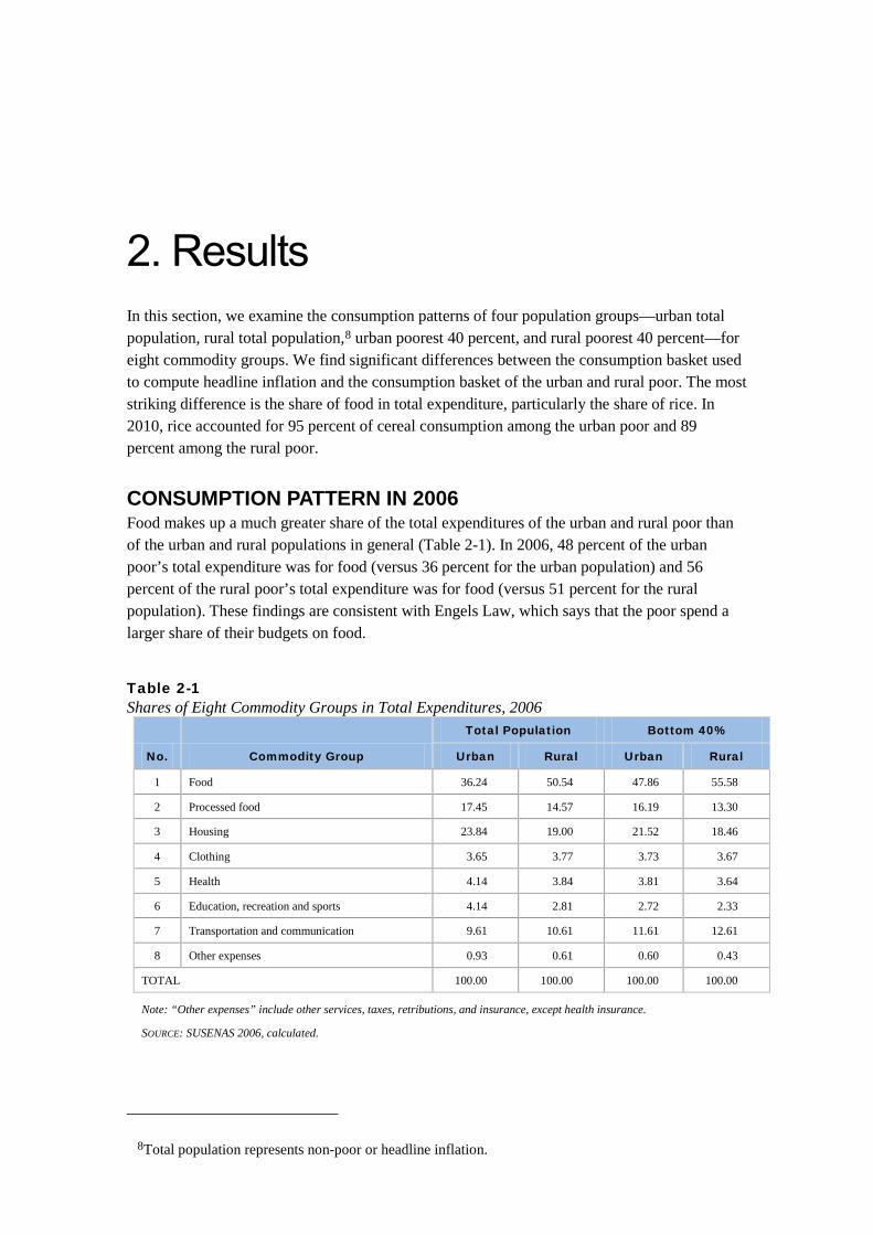
2. Results In this section, we examine the consumption patterns of four population groups—urban total population, rural total population,8 urban poorest 40 percent, and rural poorest 40 percent—for eight commodity groups. We find significant differences between the consumption basket used to compute headline inflation and the consumption basket of the urban and rural poor. The most striking difference is the share of food in total expenditure, particularly the share of rice. In 2010, rice accounted for 95 percent of cereal consumption among the urban poor and 89 percent among the rural poor.

CONSUMPTION PATTERN IN 2006 Food makes up a much greater share of the total expenditures of the urban and rural poor than of the urban and rural populations in general (Table 2-1). In 2006, 48 percent of the urban poor’s total expenditure was for food (versus 36 percent for the urban population) and 56 percent of the rural poor’s total expenditure was for food (versus 51 percent for the rural population). These findings are consistent with Engels Law, which says that the poor spend a larger share of their budgets on food.

Table 2-1 Shares of Eight Commodity Groups in Total Expenditures, 2006

No. Commodity Group

Total Population Bottom 40%

Urban Rural Urban Rural

1 Food 36.24 50.54 47.86 55.58

2 Processed food 17.45 14.57 16.19 13.30

3 Housing 23.84 19.00 21.52 18.46

4 Clothing 3.65 3.77 3.73 3.67

5 Health 4.14 3.84 3.81 3.64

6 Education, recreation and sports 4.14 2.81 2.72 2.33

7 Transportation and communication 9.61 10.61 11.61 12.61

8 Other expenses 0.93 0.61 0.60 0.43

TOTAL 100.00 100.00 100.00 100.00

Note: “Other expenses” include other services, taxes, retributions, and insurance, except health insurance.

SOURCE: SUSENAS 2006, calculated.

8Total population represents non-poor or headline inflation.

6 C P I F O R T H E P O O R I N I N D O N E S I A

For all population groups, housing claimed the biggest share of nonfood expenditure. Spending on housing does not follow the pattern for spending on food. In 2006, the urban poor spent a slightly lower proportion of their total expenditures on housing (21 percent) than did the general urban population (24 percent), while the rural poor spent almost the exact same proportion on housing (18.5 percent) as did the general rural population (19 percent).

Education claimed about the same share of urban and rural poor total expenditure (2.72 percent and 2.33 percent). The share of education in the total expenditures of non-poor urban dwellers was nearly double that (4.14 percent).

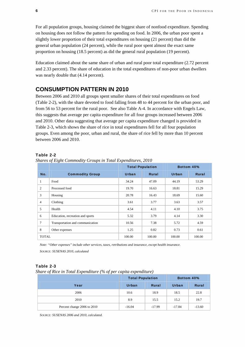
CONSUMPTION PATTERN IN 2010 Between 2006 and 2010 all groups spent smaller shares of their total expenditures on food (Table 2-2), with the share devoted to food falling from 48 to 44 percent for the urban poor, and from 56 to 53 percent for the rural poor. See also Table A-4. In accordance with Engels Law, this suggests that average per capita expenditure for all four groups increased between 2006 and 2010. Other data suggesting that average per capita expenditure changed is provided in Table 2-3, which shows the share of rice in total expenditures fell for all four population groups. Even among the poor, urban and rural, the share of rice fell by more than 10 percent between 2006 and 2010.

Table 2-2 Shares of Eight Commodity Groups in Total Expenditures, 2010

No. Commodity Group

Total Population Bottom 40%

Urban Rural Urban Rural

1 Food 34.24 47.09 44.19 53.29

2 Processed food 19.70 16.63 18.81 15.29

3 Housing 20.78 16.43 18.69 15.60

4 Clothing 3.61 3.77 3.63 3.57

5 Health 4.54 4.11 4.10 3.75

6 Education, recreation and sports 5.32 3.79 4.14 3.30

7 Transportation and communication 10.56 7.38 5.72 4.59

8 Other expenses 1.25 0.82 0.73 0.61

TOTAL 100.00 100.00 100.00 100.00

Note: “Other expenses” include other services, taxes, retributions and insurance, except health insurance.

SOURCE: SUSENAS 2010, calculated

Table 2-3 Share of Rice in Total Expenditure (% of per capita expenditure)

Year

Total Population Bottom 40%

Urban Rural Urban Rural

2006 10.6 18.9 18.5 22.8

2010 8.9 15.5 15.2 19.7

Percent change 2006 to 2010 -16.04 -17.99 -17.84 -13.60

SOURCE: SUSENAS 2006 and 2010, calculated.

R E S U L T S 7

As the poor increase their income, they tend to buy higher-value food goods and a wider variety of food. Evidence of this trend in Indonesia can be seen in changes in the share of the total budget devoted to processed food (Tables 2-1 and 2-2). Over the 2006-2010 period, the share of the budget devoted to processed food increased for all four population groups—from 16 to 19 percent for the urban poor, and from 13 to 15 percent for the rural poor.

The declining share of rice is consistent with this trend and in keeping with the declining share of cereals in total expenditure. Over the past 40 years the share of cereals (i.e., rice, tubers, maize) in the total household budget has fallen at about 0.02 percent per year. Among the urban and rural poor, the decline in the share of cereals accelerated after the economic crisis of 1998-1999. In 1969, the share was 42 percent; by 2008 it was only 10 percent among the urban poor and 15 percent among the rural poor.9

CONSUMPTION OF NONFOOD ITEMS Spending on the most important nonfood commodity—housing—fell between 2006 and 2010 (Tables 2-1 and 2-2). The share of the budget devoted to housing fell from 25 to 19 percent for the urban poor, and from 20 to 15 percent for the rural poor. The reasons for this decline are unclear and deserve more analysis. Meanwhile, spending on education rose substantially between 2006 and 2010. Between these two years the share of the budget devoted to education rose from 2 to 4 percent for the urban poor, and from 1.5 to 3 percent for the rural poor. This suggests that as the incomes of the poor rise, they tend to invest more in their children’s’ future.

THE APPROPRIATE CONSUMPTION BASKET Our findings regarding differences in the consumption patterns of the poor and non-poor in Indonesia suggest the importance of having an appropriate consumption basket for each group for each period of time. See, e.g., Table A-3. The consumption patterns of the urban and rural poor change over time, as do the rates of inflation in food and nonfood commodities. Using different consumption patterns (i.e., consumption weights in 2006 vis-à-vis in 2010), we will find different levels of inflation for each period of time.

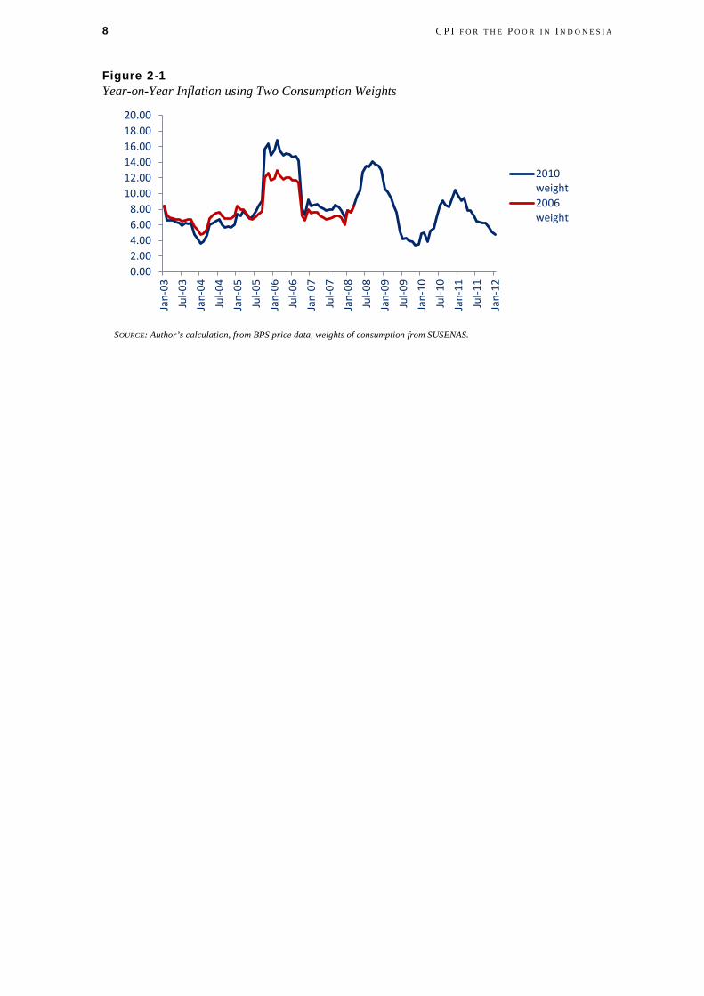
Figure 2-1 shows that the rate of inflation is relatively sensitive to the consumption basket used to weight the price level. When we compare the 2010 weight and the 2006 weight, we can see that using the 2010 (recent SUSENAS) consumption basket will overweight the price level and lead to higher inflation in the earliest years. To minimize this problem we reconstruct the inflation rate using two index years: (1) 2006 to proxy the level of consumption basket before 2008, and (2) 2010 to proxy 2009-2012.10

9 Original numbers (1969-2010) from Papanek (2011); changes overtime calculated 10 This decision to choose the two years is due to practical and subjective research decision. We

believe the best way to get an exact inflation rate is to use a different index each year. However, even BPS adjusts its index every few years.

8 C P I F O R T H E P O O R I N I N D O N E S I A

Figure 2-1 Year-on-Year Inflation using Two Consumption Weights

SOURCE: Author’s calculation, from BPS price data, weights of consumption from SUSENAS.

0.002.004.006.008.00

10.0012.0014.0016.0018.0020.00

Jan-

03Ju

l-03

Jan-

04Ju

l-04

Jan-

05Ju

l-05

Jan-

06Ju

l-06

Jan-

07Ju

l-07

Jan-

08Ju

l-08

Jan-

09Ju

l-09

Jan-

10Ju

l-10

Jan-

11Ju

l-11

Jan-

12

2010weight2006weight

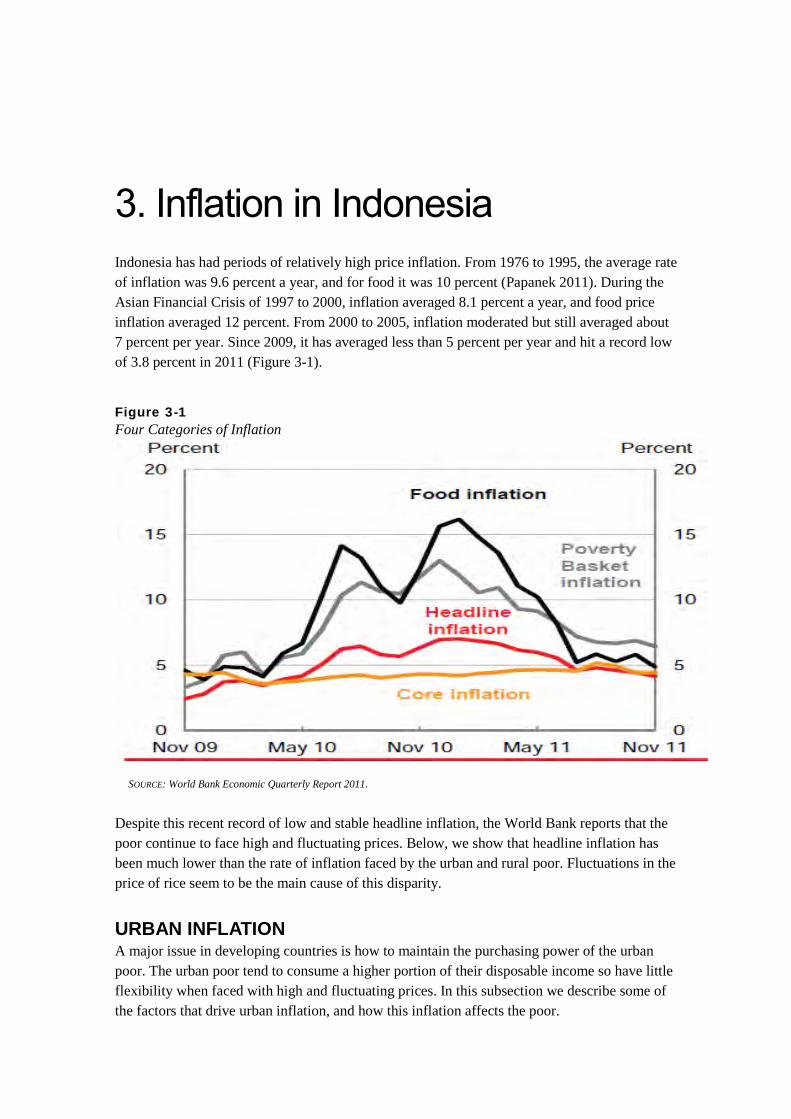
3. Inflation in Indonesia Indonesia has had periods of relatively high price inflation. From 1976 to 1995, the average rate of inflation was 9.6 percent a year, and for food it was 10 percent (Papanek 2011). During the Asian Financial Crisis of 1997 to 2000, inflation averaged 8.1 percent a year, and food price inflation averaged 12 percent. From 2000 to 2005, inflation moderated but still averaged about 7 percent per year. Since 2009, it has averaged less than 5 percent per year and hit a record low of 3.8 percent in 2011 (Figure 3-1).

Figure 3-1 Four Categories of Inflation

SOURCE: World Bank Economic Quarterly Report 2011.

Despite this recent record of low and stable headline inflation, the World Bank reports that the poor continue to face high and fluctuating prices. Below, we show that headline inflation has been much lower than the rate of inflation faced by the urban and rural poor. Fluctuations in the price of rice seem to be the main cause of this disparity.

URBAN INFLATION A major issue in developing countries is how to maintain the purchasing power of the urban poor. The urban poor tend to consume a higher portion of their disposable income so have little flexibility when faced with high and fluctuating prices. In this subsection we describe some of the factors that drive urban inflation, and how this inflation affects the poor.

1 0 C P I F O R T H E P O O R I N I N D O N E S I A

Figure 3-2 shows that inflation for the poor (the lowest 40 percent) is higher and more persistent than headline inflation. The poor suffer higher rates of inflation because their consumption basket is different from the non-poor basket, which puts more weight on prepared food and nonfood expenditures. The consumption basket for the poor places much more weight on food. For the poor the share of nonfood items in the basket is only about one half of the non-poor consumption bundle.

Figure 3-2 Two Inflation Indices, January 2002–January 2012 (yoy)

SOURCE: Author’s calculation.

Indonesia experienced three spikes in inflation over the period 2002-2012 (Figure 3-2). These spikes reflect (1) a domestic food and fuel price increase in 2005, (2) the global food and fuel crisis of 2008, and (3) and the rising price of food in 2010 to 2011.

One of the sharpest price rises of the past 10 years occurred in the 2004-2006 period. This spike was caused mainly by a rise in food prices, especially a double-digit rise in cereal prices beginning in January 2005. The government’s decision in 2005 to reduce fuel subsidies led to skyrocketing food prices and the rate of food inflation exceeded 20 percent per year between 2005 and 2007. Inflation started cooling down in October 2006 after a large drop in the cost of prepared food and household utilities. The rate of inflation for the poor, however, remained high until it converged with headline inflation in January 2008.Overall, the rate of inflation for the poor remained above 11 percent until May 2009.

Apparently, urban inflation in all indices is sensitive to a combination of prices for prepared foods, which constitute 10.8 percent to 12 percent of budgets, and for utilities (fuel, electricity, and water). The headline inflation rate certainly holds a much higher correlation than the inflation for the poor as when the prepared food prices start to drop significantly, the headline inflation also immediately declines.

In the July 2010- July 2011 period, the price of cereal increased an average of 17 percent (yoy); in addition, food products with volatile prices also have been climbing up as occurred in 2005. Undoubtedly this hurt the poor more than the non-poor; the bottom quintile of income

0.00

2.00

4.00

6.00

8.00

10.00

12.00

14.00

16.00

18.00

20.00

Jan

2003

Jun

2003

Nop

200

3Ap

r 200

4Se

p 20

04Fe

b 20

05Ju

l 200

5De

s 200

5M

ei 2

006

Okt

200

6M

ar 2

007

Agus

t…Ja

n 20

08Ju

n 20

08N

op 2

008

Apr 2

009

Sep

2009

Feb

2010

Jul 2

010

Des 2

010

Mei

201

1O

kt 2

011

Headline

40 percent

I N F L A T I O N I N I N D O N E S I A 1 1

distribution experienced 13 percent inflation while headline inflation was a moderate 7 percent. Still, when compared to the price shocks of 2005, inflation was low as the prices of prepared food remained relatively stable and inflationary pressure from fuel, electricity and water was extremely low.

Table 3-1 Inflation, December 2003–2011 (yoy)

Year 40% Headline

2003 4.2 5.06

2004 5.7 11.24

2005 15.5 17.11

2006 9.9 6.60

2007 7.00 6.60

2008 13.01 13.86

2009 3.52 2.78

2010 10.43 6.96

2011 5.15 3.79

SOURCE: Warta IHK various years, authors calculation.

Table 3-1 summarizes annual changes in headline inflation and inflation for the poor (the lowest 40 percent) for the period 2003 to 2011. Over the long term the average annual rates of inflation are not that different, but we see substantial differences when we compare year by year. For example, in 2006 and 2010 the poor experienced much higher inflation than recorded in headline figures. This suggests that it is important to identify how and when inflation rates for the poor exceed those recorded by the official CPI. Food prices figure heavily here. Prices for cereal products, including rice, jumped 29.13 percent in December 2006, and 26.91 percent in December 2010 (yoy).

While the poor suffer disproportionately when food prices rise, the rich face initially higher inflation whenever the prices for electricity and fuel rise rapidly. When electricity prices rose sharply in 2003, the inflation rate for the poor was half that of the non-poor in the month in question. But fuel price increases generally flow through to other prices. For instance, the price of cereals and rice positively correlated with the price of fuel. In December 2005 the price cereal inflation was 26 percent after a large increase in fuel prices.

RURAL INFLATION We derived our rural CPI measure for this study from the household consumption index of the Farmers Terms of Trade.11These data are published monthly by BPS and are available in the Statistical Yearbook. In this section, we construct the rural poor CPI index by multiplying the Indices of Consumer Prices Paid by Farmers on farmers’ terms of trade data with the weights of commodity categories obtained for the lowest 40 percent of rural population.

11Commonly known as Indeks Konsumsi Rumah Tangga (IKRT). We extracted it from the Farmers’ Terms of Trade Index. The index measures prices paid by medium-level farmers. Table A-6 reports the changes the price indices for food and processed food for rural households, 2003-2007

1 2 C P I F O R T H E P O O R I N I N D O N E S I A

The base year for the rural CPI is 2007. Data from previous years are rebased to 2007 to ensure data continuity. Similar to the rural price indices, all commodity groups’ price indices of the rural poor CPI are based on 100 in 2007. The BPS has changed the number of commodity groups in its reports. From 2003 until 2007, it reported on four groups (food, housing, clothing, and miscellaneous goods and services). Since 2008 it has reported on seven (food; prepared food; housing; clothing; health; education, recreation and sports; and transportation and communication).

To reflect this change, we made weight adjustments as follows. First, we derived weights from the consumption module of the 2006 and 2010 SUSENAS. We then used the 2006 weights to count the rural poor CPI from 2003 until 2008. Second, we used 2010 weights to count rural poor CPI from 2009 until January 2012. Third, because the 2003–2007 data had only four categories, we readjusted to seven categories.12 The available weights consist of eight categories. We ignore the “other expenses” category’s weights for 2007 until January 2012 because of its small incremental value, and continue to use the data format with seven categories. Table 3-2 shows the consumption basket we use in constructing the rural poor CPI compared to the consumption basket used in the BPS index (weights before 2007).

Table 3-2 Consumption Shares of the Rural Poor (%)

No. Commodity Group Pre-2007 2006 2010

1 Food 69 56 53

2 Processed food Na 13 15

3 Housing 19 19 16

4 Clothing 4 4 4

5 Health Na 4 4

6 Education, recreation and sports Na 2 3

7 Transportation and communication Na 3 5

8 Other expenses 8.6 0.5 0.1

Total 100 100 100

NOTES: A breakdown of the rural poor and non-poor inflation index is presented in Table A-5 in the appendix. Shares before 2007 are the original consumption sharesand non-2007 published by BPS with only four price items.

SOURCE: Authors’ calculation. Table A-7 presents our calculated Price Index for the Rural Poor along with our estimated rates of inflation from 2003 through 2011.

12We summed the food and processed food weights on the 2006 SUSENAS to get food weights. Then, to get the miscellaneous weights, we summed health, education, recreation, sports, and transport and communication categories.

I N F L A T I O N I N I N D O N E S I A 1 3

Table 3-3 Rural Headline Inflation and Inflation for Rural Poor, 2005-2011

Year Rural Headline Rural Poor (40%)

2005 11.41 11.20

2006 14.67 14.47

2007 8.36 8.78

2008 13.04 12.80

2009 7.41 7.18

2010 5.64 6.12

2011 7.77 7.19

SOURCE: Authors’ calculation. During the 2007 to 2011 period, food made the largest contribution to the rural CPI for the poor (in relative terms; see Table 3-4). Among the seven commodities, housing had the lowest inflation (4 percent). Prices for transport and communication increased dramatically in 2010, resulting in an average annual inflation rate of 16 percent. The rate of inflation of food increased dramatically in 2008, but then started to decline.

Table 3-4 Rural Poor CPI, Contribution by Category, 2007–2011

Commodity 2007 2008 2009 2010 2011

Food 55.60 64.30 68.86 70.84 75.70

Processed food 13.30 14.47 15.76 19.39 20.42

Housing 18.50 21.05 22.85 20.18 21.23

Clothing 3.70 4.02 4.37 4.44 4.71

Health 3.60 3.93 4.17 4.49 4.65

Education, recreation, and sports 2.30 2.50 2.65 3.90 4.02

Transportation and communication 2.60 2.90 2.88 5.13 5.21

SOURCE: Authors’ calculation. To understand the price behavior of the commodities, we also calculate the rural CPI for the poor for the period January 2011 until January 2012. The monthly change in value for each category is similar to the results reported above, with the food category fluctuating the most. No other categories show a significant change from the findings reported above. In fact, the price of all commodities (except food) seems to be stable over time. At the start of the year (January to March) the rural poor CPI for food tends to be high and then declines in the middle of the year (April to May). From June to December the rural poor CPI for food increases steadily.

A key factor in food price fluctuations is the harvest time. At the beginning of the year, the price of rice (which has the biggest share for food categories) tends to be lower than in other months. This is the lean season for farmers. The price reaches its lowest point in April–May, the main harvest time for farmers. From June until August, the price started to move up as the rice stocks begin to fall.

1 4 C P I F O R T H E P O O R I N I N D O N E S I A

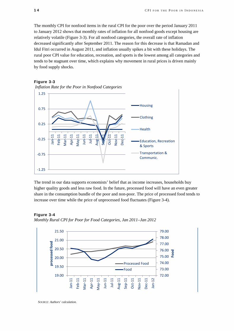
The monthly CPI for nonfood items in the rural CPI for the poor over the period January 2011 to January 2012 shows that monthly rates of inflation for all nonfood goods except housing are relatively volatile (Figure 3-3). For all nonfood categories, the overall rate of inflation decreased significantly after September 2011. The reason for this decrease is that Ramadan and Idul Fitri occurred in August 2011, and inflation usually spikes a bit with these holidays. The rural poor CPI value for education, recreation, and sports is the lowest among all categories and tends to be stagnant over time, which explains why movement in rural prices is driven mainly by food supply shocks.

Figure 3-3 Inflation Rate for the Poor in Nonfood Categories

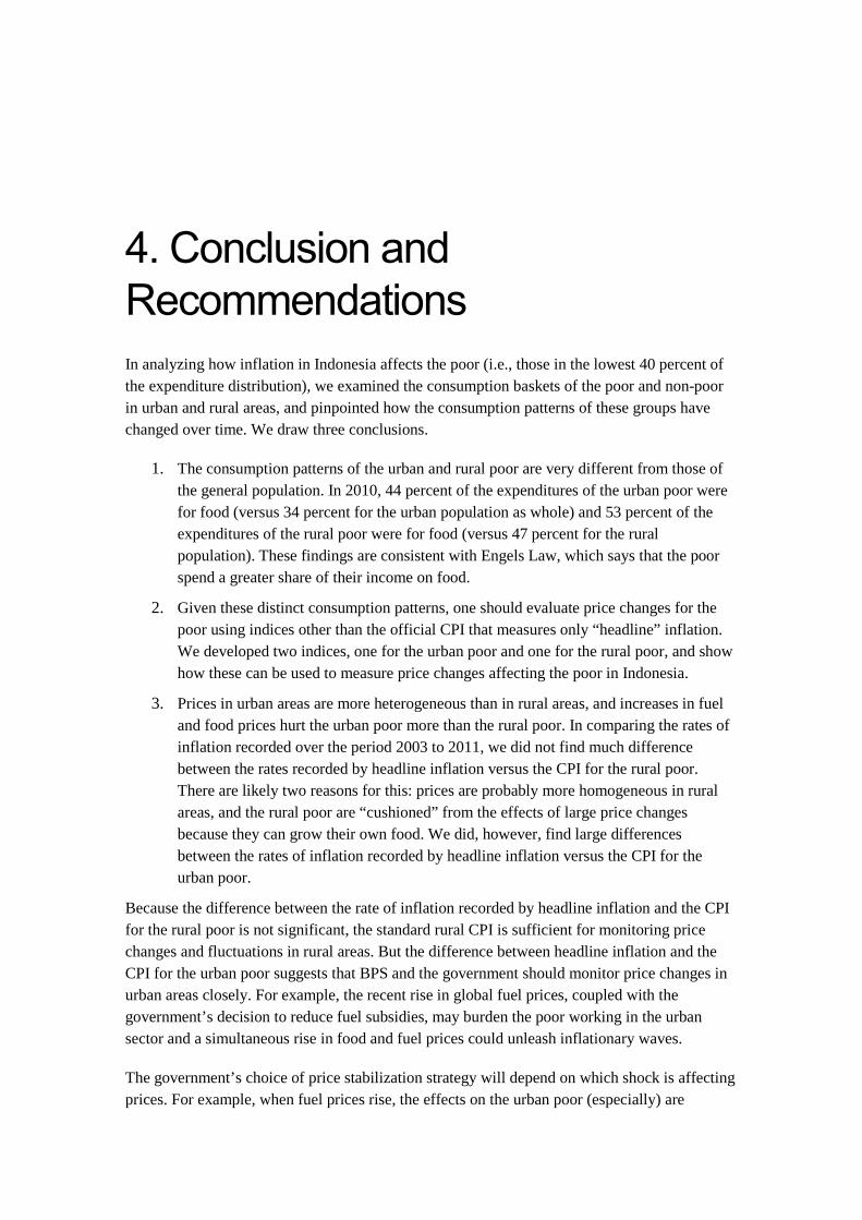
The trend in our data supports economists’ belief that as income increases, households buy higher quality goods and less raw food. In the future, processed food will have an even greater share in the consumption bundle of the poor and non-poor. The price of processed food tends to increase over time while the price of unprocessed food fluctuates (Figure 3-4).

Figure 3-4 Monthly Rural CPI for Poor for Food Categories, Jan 2011–Jan 2012

SOURCE: Authors’ calculation.

-1.25

-0.75

-0.25

0.25

0.75

1.25

Jan-

11

Feb-

11

Mar

-11

Apr-

11

May

-11

Jun-

11

Jul-1

1

Aug-

11

Sep-

11

Oct

-11

Nov

-11

Dec-

11

Housing

Clothing

Health

Education, Recreation& Sports

Transportation &Communic.

72.00

73.00

74.00

75.00

76.00

77.00

78.00

79.00

19.00

19.50

20.00

20.50

21.00

21.50

Jan-

11

Feb-

11

Mar

-11

Apr-

11

May

-11

Jun-

11

Jul-1

1

Aug-

11

Sep-

11

Oct

-11

Nov

-11

Dec-

11

Jan-

12

Food

proc

esse

d fo

od

Processed FoodFood

I N F L A T I O N I N I N D O N E S I A 1 5

URBAN AND RURAL INFLATION This subsection describes the movement of prices in urban and rural areas and in income groups over time.13 Changes in monthly inflation (yoy) for the urban poor, rural poor, rural non-poor, and urban non-poor show that inflation in urban and rural areas was strikingly different from January 2009 to January 2012 (Figure 3-5). The non-poor in urban areas (headline) consistently enjoyed lower prices compared to the other three groups.14 In contrast, the poor in urban areas paid the highest prices as their price levels exceeded general rural inflation in February 2010.

Figure 3-5 Urban and Rural Inflation, January 2009-January 2012

SOURCE: Authors’ calculation.

The gap between prices paid by the urban poor and non-poor is wide (except for January-April 2010), while the gap between prices paid by the rural poor and non-poor is negligible and the price co-movements surprisingly close. We also observe that the relation between prices received by the urban poor and the ones paid by the rural poor changes over time; initially prices in rural areas were slightly higher during January-April 2009, but urban prices rose from then on. Prices peaked in January 2011, and general prices for all groups have been declining for the past 12 months. In January 2012, for the first time, prices in rural areas for poor and non-poor were slightly lower than the headline CPI—which means that prices in rural areas fell faster than in urban areas.

Breaking down the inflation items allows us to tease out the primary cause of inflation differences. Using the monthly food price inflation as shown in Figure 3-6 we can see that the point where urban poor prices start to diverge from the rural poor in Figure 3-5 is exactly where the gap between the urban poor food price and rural food price emerges. The gap persists until food prices peak in January 2011.

13 Examination of pre-2008 inflation was difficult because we had only monthly data for the 2008-2012 period.

14 Urban-rural inflation (poor and non poor) from 2007-2011 is compared in Table A-8.

2.00

0.00

2.00

4.00

6.00

8.00

10.00

12.00

14.00

Jan-

09

Apr-

09

Jul-0

9

Oct

-09

Jan-

10

Apr-

10

Jul-1

0

Oct

-10

Jan-

11

Apr-

11

Jul-1

1

Oct

-11

Jan-

12

urban poor

Rural poor

rural non poor

headline

1 6 C P I F O R T H E P O O R I N I N D O N E S I A

The similarity in the trend again emphasizes our previous remark that price movements of goods consumed by the poor are sensitive to the changes in food prices. Rising food prices in urban areas have broadened the gap between rural and urban. Our CPI breakdown data indicate that the increase in urban prices starting from January 2010 is closely related to the increase in cereal prices and movement of volatile price.

Figure 3-6 Urban and Rural Food Inflation Comparisons (yoy)

` SOURCE: Authors’ calculation.

As Figure 3-6 shows, when the cereal price is relatively low, the urban and rural food index difference is very small and as the cereal price rises, the gap between food prices paid by urban and rural dwellers widens. Both indexes start to converge around April 2011 as cereal prices start to go down.15

15 The drop in the food price index in rural areas between December 2009 and January 2010 is intriguing. We worked out a three-month average to reveal more about dynamics and seasonality but the trend remains. One possible explanation is that the BPS cereal price index is biased to urban areas. But when we used several alternative indicators for rural areas (e.g., price of rice at farmers’ level for several levels of quality) we could not find a satisfying explanation for the deflation.

-3.00

3.00

9.00

15.00

21.00

27.00

Jan-

09M

ar-0

9M

ay-0

9Ju

l-09

Sep-

09N

ov-0

9Ja

n-10

Mar

-10

May

-10

Jul-1

0Se

p-10

Nov

-10

Jan-

11M

ar-1

1M

ay-1

1Ju

l-11

Sep-

11N

ov-1

1Ja

n-12

Index Rural

index urban

cereal index

4. Conclusion and Recommendations In analyzing how inflation in Indonesia affects the poor (i.e., those in the lowest 40 percent of the expenditure distribution), we examined the consumption baskets of the poor and non-poor in urban and rural areas, and pinpointed how the consumption patterns of these groups have changed over time. We draw three conclusions.

1. The consumption patterns of the urban and rural poor are very different from those of the general population. In 2010, 44 percent of the expenditures of the urban poor were for food (versus 34 percent for the urban population as whole) and 53 percent of the expenditures of the rural poor were for food (versus 47 percent for the rural population). These findings are consistent with Engels Law, which says that the poor spend a greater share of their income on food.

2. Given these distinct consumption patterns, one should evaluate price changes for the poor using indices other than the official CPI that measures only “headline” inflation. We developed two indices, one for the urban poor and one for the rural poor, and show how these can be used to measure price changes affecting the poor in Indonesia.

3. Prices in urban areas are more heterogeneous than in rural areas, and increases in fuel and food prices hurt the urban poor more than the rural poor. In comparing the rates of inflation recorded over the period 2003 to 2011, we did not find much difference between the rates recorded by headline inflation versus the CPI for the rural poor. There are likely two reasons for this: prices are probably more homogeneous in rural areas, and the rural poor are “cushioned” from the effects of large price changes because they can grow their own food. We did, however, find large differences between the rates of inflation recorded by headline inflation versus the CPI for the urban poor.

Because the difference between the rate of inflation recorded by headline inflation and the CPI for the rural poor is not significant, the standard rural CPI is sufficient for monitoring price changes and fluctuations in rural areas. But the difference between headline inflation and the CPI for the urban poor suggests that BPS and the government should monitor price changes in urban areas closely. For example, the recent rise in global fuel prices, coupled with the government’s decision to reduce fuel subsidies, may burden the poor working in the urban sector and a simultaneous rise in food and fuel prices could unleash inflationary waves.

The government’s choice of price stabilization strategy will depend on which shock is affecting prices. For example, when fuel prices rise, the effects on the urban poor (especially) are

1 8 C P I F O R T H E P O O R I N I N D O N E S I A

persistent and prolonged.16 The government should therefore stand ready to provide cash or other transfers to the urban poor if inflation rises too much. And the growing share of processed food in the household expenditures of the urban and rural poor suggests that the government can help stabilize prices not only by focusing on the price of rice and other volatile raw foods, like chilies and onions, but also by lowering the cost of food distribution by improving infrastructure for food wholesalers and the supply chain system, especially for connection to rural areas.

16 The CPI for the poor jumped to almost to the same level as headline inflation whenever the fuel subsidy was cut. This month-to-month inflation remained high for the next three months, but for the non-poor (headline inflation) it was registered as only a one-time shock.

Bibliography Asra, A. 2001. Urban-Rural Differences in Cost of Living and Their Impact on Poverty

Measures. Asian Development Bank.

Asian Development Bank. 2008. Special Report: Food Prices and Inflation in Developing Asia. Economic and Research Department.

Delisle, H. 1990. Patterns of Urban Food Consumption in Developing Countries: Perspectives from the 1990’s. Rome: FAO and Universite de Montreal.

Frankenberg, E., D., Thomas and K. Beegle. 1999. The Real Cost of Indonesia’s Economic Crisis: Preliminary Findings from the Indonesia Family Life Surveys. Rand Corporation.

Rao and Komala. 1997. Are Prices Higher for the Poor? Heterogeneity and Real Inequality in Rural Karnataka. Economic and Political Weekly, Vol. 32, No.48.

McCulloch. N. 2008. Rice Prices and Poverty in Indonesia. Bulletin of Indonesian Economic Studies, Vol. 44, No 1.

Papanek. 2011. Inflation and the Poor. TNP2K working paper. Unpublished memo.

Ravallion and Van der Walle. 1989. Cost of Living Differences between Urban and Rural Areas in Indonesia. Policy, Planning and Research working papers WPS 341, World Bank.

Rao. 2000. Price Heterogeneity and ‘Real’ Inequality: A Case Study of Prices and Poverty in Rural South India. Review of Income and Wealth, Vol. 42, No 2.

Sigit, H. and Sudarti Surbakti. 1999. Social Impact of the Economic Crisis in Indonesia. Presented at Finalization Conference of Assessing the Social Impact of the Financial Crisis in Selected Asian Developing Countries.

Sugema, et.al. 2010. The Impact of Inflation on Rural Poverty Indonesia: An Econometric Approach. . European Research Journal of Finance and Economics, 50-2887 issue 58.

Block, S.A., C. P. Timmer, and D. Dawe. 2011. Long Run Dynamics of Rice Consumption 1960-2050. In International Rice Research Institute 50th Anniversary volume.

Appendix. Detailed Data Table A-1 Detailed Consumption Distribution, 2006 and 2010

No Commodity

Group

2006 2010

Total Population Bottom 40% Total Population Bottom 40%

Urban Rural Urban Rural Urban Rural Urban Rural

F O O D

1 Rice 10.6 18.9 18.5 22.8 8.9 15.5 15.2 19.7

2 Cereal, cassava, and related products (excl. rice)

0.7 2.2 1.0 2.8 0.7 1.8 0.9 2.3

3 Meat and meat products

1.9 1.4 0.9 1.1 2.0 1.7 1.2 1.2

4 Fresh fish 3.5 4.1 3.2 3.9 3.2 4.0 2.9 3.8

5 Preserved fish 1.0 1.6 1.4 1.8 0.9 1.5 1.5 1.8

6 Eggs, milk and related products

3.3 2.3 2.6 2.0 3.4 2.7 2.9 2.4

7 Vegetables 4.4 6.1 6.3 6.6 4.0 5.8 5.5 6.7

8 Beans and nuts 1.9 2.1 3.0 2.2 1.8 2.0 2.7 2.4

9 Fruits 2.0 2.0 1.6 1.8 2.4 2.6 2.0 2.3

10 Spices 1.4 1.9 1.8 2.0 1.2 1.5 1.6 1.7

11 Fats and oils 1.9 2.9 2.7 3.2 2.1 2.9 2.9 3.3

12 Other 3.8 5.0 5.1 5.4 3.7 5.0 4.8 5.6

13 BF: prepared food 10.0 6.7 8.9 6.1 12.3 8.6 11.1 7.8

14 BF; non alcohol beverages

1.6 0.9 1.2 0.8 2.1 1.4 1.8 1.2

15 BF: tobacco and alcohol beverages

5.9 7.0 6.1 6.5 5.3 6.7 5.8 6.4

SUBTOTAL, Food 52.50 53.7 65.1 64.1 68.9 63.7 63.0 68.6

N O N F O O D

H O U S I N G

16 Cost for housing 12.7 8.3 9.7 7.6 11.78 7.41 9.12 6.55

17 Fuel, electricity and water

9.0 8.7 10.1 8.9 6.76 6.91 7.76 7.15

18 Household equipment 0.7 0.8 0.4 0.7 0.72 0.92 0.53 0.71

19 Household operation 1.5 1.2 1.3 1.3 1.52 1.19 1.28 1.20

A - 2 A P P E N D I X

No Commodity

Group

2006 2010

Total Population Bottom 40% Total Population Bottom 40%

Urban Rural Urban Rural Urban Rural Urban Rural

C L O T H I N G

20 Clothing for men, women and children

3.5 3.7 3.6 3.6 3.40 3.58 3.55 3.49

21 Personal effects 0.2 0.1 0.1 0.1 0.21 0.19 0.08 0.08

H E A L T H

22 Health services 1.5 1.4 1.0 1.2 1.97 1.68 1.43 1.32

23 Medicines 0.5 0.4 0.4 0.4 0.47 0.40 0.40 0.37

24 Beauty treatment and cosmetics

2.2 2.0 2.3 2.1 2.10 2.03 2.27 2.06

E R

25 Education 2.2 0.9 1.3 0.8 3.14 1.89 2.65 1.88

26 Courses and training 0.0 0.0 0.0 0.0 0.10 0.04 0.06 0.03

27 Educational equipment

0.7 0.5 0.7 0.5 0.70 0.58 0.74 0.59

28 Recreation and sports 1.2 1.4 0.7 1.0 1.38 1.28 0.70 0.79

T R A N S P O R T A T I O N A N D C O M M U N I C A T I O N

29 Transport 6.4 3.7 3.2 2.3 6.15 4.46 3.92 3.26

30 Communication and delivering

2.5 0.5 0.4 0.2 2.91 1.55 1.61 1.09

31 Transport equipment and support

0.7 0.7 0.0 0.1 1.44 1.36 0.18 0.24

32 Finance services 0.0 0.0 0.0 0.0 0.06 0.01 0.01 0.00

O T H E R

33 Other services 0.1 0.1 0.1 0.1 0.07 0.07 0.06 0.06

34 Taxes and insurance (excl. health)

0.9 0.5 0.6 0.4 1.17 0.75 0.67 0.55

SUBTOTAL, nonfood 47.50 46.3 34.9 35.9 31.1 36.3 37.0 31.4

TOTAL Expenditure 100.00 100.0 100.0 100.0 100.0 100.0 100.0 100.0

SOURCE: SUSENAS 2006 and 2010, calculated.

D E T A I L E D D A T A A - 3

Table A-2 Commodity Groups in Warta IHK and SUSENAS Consumption Items

No. Warta IHK Commodity Groups SUSENAS Consumption Items

1 Food: Cereal, Cassava & Related Products OK, weight for rice is separated from cereal and cassava products and put into a new commodity group.

2 Food: Meat and Meat Products OK

3 Food: Fresh Fish OK

4 Food: Preserved Fish OK

5 Food: Eggs, Milk and Related Products OK

6 Food: Vegetables OK

7 Food: Beans and Nuts OK

8 Food: Fruits OK

9 Food: Spices OK

10 Food: Fats and Oils OK

11 Food: Other OK

12 BF: Prepared Food OK

13 BF: Non Alcohol Beverages OK

14 BF: Tobacco and Alcohol Beverages OK

15 Housing: Cost for Housing OK

16 Housing: Fuel, Electricity and Water OK

17 Housing: Household Equipment OK

18 Housing: Household Operation OK

19 Clothing: For Men The consumption items in SUSENAS 2010 differentiate between apparel for men, women, and children, but don’t differentiate fabric, hats, and footwear for men, women and children.

20 Clothing: For Women

21 Clothing: For Children

22 Clothing: Personal Effects OK

23 Health: Health Service and Medicines For this commodity groups, the study only includes health services including health insurance

24 Health: Medicines OK

25 Health: Beauty Treatment Service Not available

26 Health: Beauty Treatment and Cosmetic OK

27 ER: Education OK

28 ER: Courses and Training OK

29 ER: Educational Equipment OK

30 ER: Recreation There are expenses for recreation and sports that are put in one expense item, so that the study sums all expenses for recreation and sports into one commodity group of "Recreation and Sports"

31 ER: Sports

32 TC: Transport OK

33 TC: Communication and Delivering OK

34 TC: Transport Equipment and Support OK

35 TC: Finance Services OK (The study only include financial services, while expenses on other services, taxes, retribution and insurance are classified in 2 new commodity group, i.e. "Other Services" and "Taxes, Retributions and Insurances")

Note: "OK" means that the consumption items from SUSENAS can be classified similar to the classification of commodity groups in Warta IHK.

A - 4 A P P E N D I X

Table A-3 Comparison of Shares of Urban Consumption in the 2010 SUSENAS and CPI Weigths

No. Commodity Group

SUSENAS 2010 World Bank (2005)

Total Pop. Bottom 20% CPI weight (Urban)

Poverty Weight (Urban) Urban Rural Urban Rural

1 Cereal, cassava, and related products

9.6 17.3 19.9 24.7 5.4 29.6

2 Meat and meat products 2.0 1.7 0.9 1.0 3.6 4.4

3 Fresh fish 3.2 4.0 2.4 3.4 3.3 2.8

4 Preserved fish 0.9 1.5 1.5 1.8 0.7 0.6

5 Eggs, milk, and related products 3.4 2.7 2.5 2.2 2.2 5.7

6 Vegetables 4.0 5.8 5.8 6.8 2.1 2.6

7 Beans and nuts 1.8 2.0 3.1 2.4 1.1 3.4

8 Fruits 2.4 2.6 1.7 2.2 2.2 2.6

9 Spices 1.2 1.5 1.6 1.7 2.1 2.2

10 Fats and oils 2.1 2.9 2.9 3.4 1.7 0.9

11 Other 3.7 5.0 5.1 5.7 0.3 3.6

12 BF: prepared food 12.3 8.6 9.3 6.9 10.1 4.7

13 BF: non alcohol beverages 2.1 1.4 1.5 0.9 3.2 1.5

14 BF: tobacco and alcohol beverages

5.3 6.7 5.2 5.8 4.3 2.3

Total 53.9 63.7 63.4 69.0 42.3 66.9

SOURCE : Author’s calculation, SUSENAS consumption module

Table A-4 Shares in Eight Consumption Components, 2006 and 2010

No. Commodity

Group

2006 2010

Total Pop. Bottom 40% Total Pop. Bottom 40%

Urban Rural Urban Rural Urban Rural Urban Rural

1 Food 36.24 50.54 47.86 55.58 34.24 47.09 44.19 53.29

2 Processed food 17.45 14.57 16.19 13.30 19.70 16.63 18.81 15.29

3 Housing 23.84 19.00 21.52 18.46 20.78 16.43 18.69 15.60

4 Clothing 3.65 3.77 3.73 3.67 3.61 3.77 3.63 3.57

5 Health 4.14 3.84 3.81 3.64 4.54 4.11 4.10 3.75

6 Education, recreation etc.

4.14 2.81 2.72 2.33 5.32 3.79 4.14 3.30

7 Transport and communication

9.61 10.61 11.61 12.61 10.56 7.38 5.72 4.59

8 Other expenses 0.93 0.61 0.60 0.43 1.25 0.82 0.73 0.61

TOTAL 100 100 100 100 100 100.00 100.00 100.00

Note: Other expenses include other services, taxes, retributions, and insurance except health insurance.

SOURCE : SUSENAS consumption module 2006, 2010. The eight components are comparable to monthly price indices published by BPS.

D E T A I L E D D A T A A - 5

Table A-5 Index Breakdown for Poor and Non-poor Rural Inflation

No. Commodity

Group Pre-2007

Categories 2006 Share Categories

2010 Share Categories

Non-poor Share Categories

1 Food 69 56 53 49

2 Processed food Na 13 15 13

3 Housing 19 19 16 15

4 Clothing 4 4 4 9

5 Health Na 4 4 1

6 Education, recreation and sports

Na 2 3 7

7 Transportation & communication

Na 3 5 6

8 Other expenses 8.6 0.5 0.1 Na

TOTAL 100 100 100 100

Note: The pre-2007, 2006, and 2010 columns are our estimated rural poor inflation index breakdown; the non-poor shares (last column) is an OLS estimate of the breakdown of BPS Rural CPI index. BPS rural inflation is derived from the Household Consumption indice component in Farmers terms of trade indicator.

Table A-6 Price Movements in Rural Areas of Food and Processed Food (year on year)

Year Food Processed

Food Food

Inflation Processed

Food

2003 66.68

2004 49.34 na -26.00 Na

2005 55.14 na 11.76 Na

2006 62.95 na 14.15 Na

2007 56.83 12.62 -9.71 Na

2008 65.72 13.73 15.64 8.77

2009 70.38 14.95 7.09 8.91

2010 70.84 19.39 0.65 29.69

1st semester 2011 75.14 20.24 6.06 4.35

Total 2011 75.70 20.42 6.86 5.30

Dec 2010 75.01 19.92 - -

Jan-11 76.33 20.21 1.76 1.44

Feb-11 76.17 20.27 -0.21 0.33

Mar-11 75.76 20.35 -0.55 0.35

Apr-11 74.59 20.35 -1.53 0.02

May-11 74.34 20.41 -0.34 0.28

Jun-11 74.81 20.44 0.63 0.16

Jul-11 75.48 20.52 0.90 0.37

Aug-11 76.21 20.60 0.97 0.40

Sep-11 76.45 20.68 0.31 0.41

Oct-11 76.31 20.64 -0.18 -0.21

Nov-11 76.70 20.70 0.51 0.30

A - 6 A P P E N D I X

Year Food Processed

Food Food

Inflation Processed

Food

Dec-11 77.03 20.77 0.43 0.36

Jan-12 77.78 20.91 0.97 0.64

Table A-7 Rural Inflation

Year Rural Poor

CPI Rural CPI

Inflation:

Rural Poor Rural

Inflation

2003 88.91 85.92 na na

2004 71.35 72.22 na na

2005 79.58 80.31 11.54 11.21

2006 91.45 91.93 14.91 14.47

2007 100.00 100.00 9.35 8.77

2008 113.25 112.80 13.25 12.80

2009 121.58 120.90 7.35 7.18

2010 128.38 128.30 5.59 6.12

1st semester 2011 134.76 134.40 4.97 4.75

Total 2011 135.94 135.58 5.89 5.67

Dec 2010 133.76 133.33 - -

Jan-11 135.73 134.64 1.47 0.98

Feb-11 135.78 134.83 0.04 0.14

Mar-11 135.63 134.75 -0.11 -0.06

Apr-11 134.65 133.95 -0.73 -0.59

May-11 134.64 133.96 0.00 0.01

Jun-11 135.28 134.50 0.47 0.40

Jul-11 136.17 135.34 0.66 0.62

Aug-11 137.17 136.34 0.73 0.74

Sep-11 137.60 136.74 0.32 0.29

Oct-11 137.23 136.91 -0.27 0.12

Nov-11 137.82 137.47 0.43 0.41

Dec-11 138.35 137.52 0.38 0.04

Jan-12 139.42 138.54 0.77 0.74

D E T A I L E D D A T A A - 7

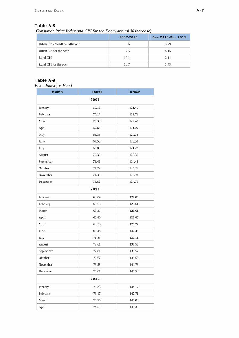
Table A-8 Consumer Price Index and CPI for the Poor (annual % increase)

2007-2010 Dec 2010-Dec 2011

Urban CPI -"headline inflation" 6.6 3.79

Urban CPI for the poor 7.5 5.15

Rural CPI 10.1 3.14

Rural CPI for the poor 10.7 3.43

Table A-9 Price Index for Food

Month Rural Urban

2 0 0 9

January 69.15 121.40

February 70.19 122.71

March 70.30 122.48

April 69.62 121.09

May 69.35 120.75

June 69.56 120.52

July 69.85 121.22

August 70.39 122.35

September 71.42 124.44

October 71.77 124.75

November 71.36 123.93

December 71.62 124.76

2 0 1 0

January 68.09 128.05

February 68.68 129.61

March 68.33 126.61

April 68.46 128.86

May 68.53 129.27

June 69.48 132.43

July 71.85 137.11

August 72.61 138.55

September 72.81 139.57

October 72.67 139.53

November 73.58 141.78

December 75.01 145.58

2 0 1 1

January 76.33 148.17

February 76.17 147.71

March 75.76 145.06

April 74.59 143.36

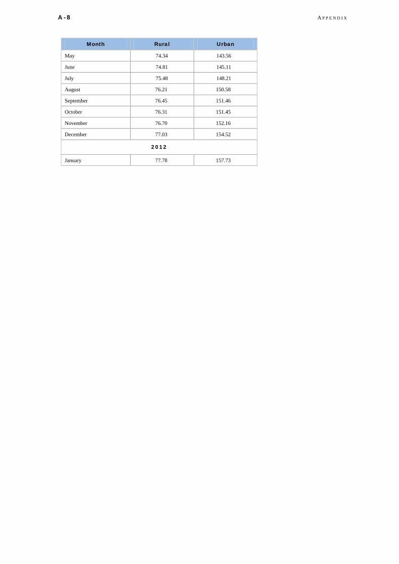
A - 8 A P P E N D I X

Month Rural Urban

May 74.34 143.56

June 74.81 145.11

July 75.48 148.21

August 76.21 150.58

September 76.45 151.46

October 76.31 151.45

November 76.70 152.16

December 77.03 154.52

2 0 1 2

January 77.78 157.73