Consumer Choice ETP Economics 101. Budget Constraint The budget constraint depicts the limit on the consumption “ bundles ” that a consumer can afford

Consumer Choice

ETP Economics 101

Budget Constraint

The budget constraint depicts the limit on the consumption “bundles” that a consumer can afford. People consume less than they desire because their

spending is constrained, or limited, by their income. The budget constraint shows the various

combinations of goods the consumer can afford given his or her income and the prices of the two goods.

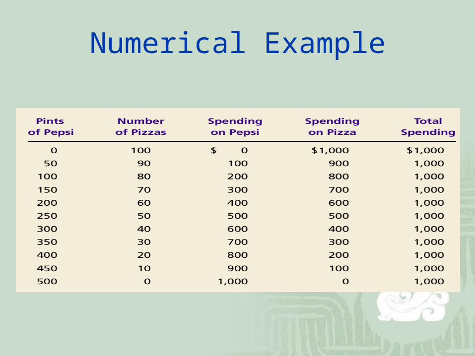
Numerical Example

Quantityof Pizza

Quantityof Pepsi

0

Consumer’sbudget constraint

500B

100

A

Copyright©2004 South-Western

Slope versus Relative Price

The slope of the budget constraint line equals the relative price of the two goods, that is, the price of one good compared to the price of the other.

It measures the rate at which the consumer can trade one good for the other.

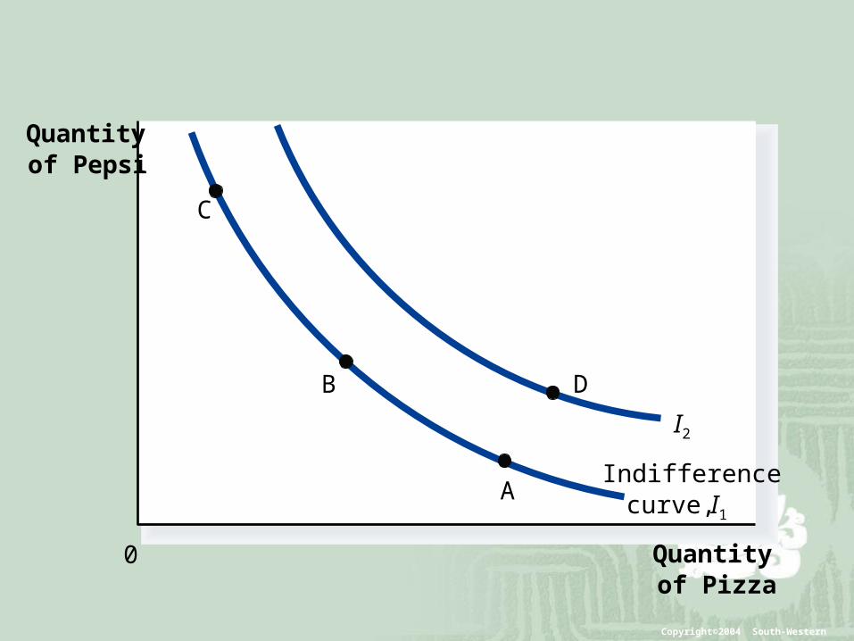
Preference and Indifference Curve

A consumer’s preference among consumption bundles may be illustrated with indifference curves.

An indifference curve is a curve that shows consumption bundles that give the consumer the same level of satisfaction.

Quantityof Pizza

Quantityof Pepsi

0

Indifferencecurve, I1

I2

C

B

A

D


Marginal Rate of Substitution

The Consumer’s Preferences The consumer is indifferent, or equally happy, with the

combinations shown at points A, B, and C because they are all on the same curve.

The Marginal Rate of Substitution The slope at any point on an indifference curve is the

marginal rate of substitution. It is the rate at which a consumer is willing to trade one good for

another. It is the amount of one good that a consumer requires as

compensation to give up one unit of the other good.

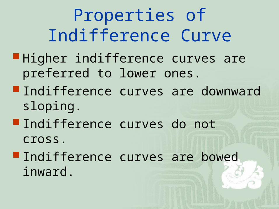
Properties of Indifference Curve

Higher indifference curves are preferred to lower ones.

Indifference curves are downward sloping. Indifference curves do not cross. Indifference curves are bowed inward.

Property 1

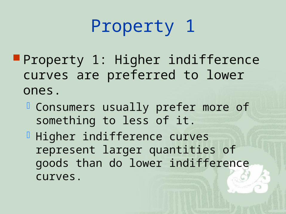
Property 1: Higher indifference curves are preferred to lower ones. Consumers usually prefer more of something to

less of it. Higher indifference curves represent larger

quantities of goods than do lower indifference curves.

Property 2

Property 2: Indifference curves are downward sloping. A consumer is willing to give up one good only if he or

she gets more of the other good in order to remain equally happy.

If the quantity of one good is reduced, the quantity of the other good must increase.

For this reason, most indifference curves slope downward.

Property 3

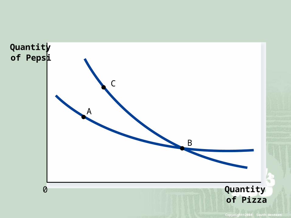
Property 3: Indifference curves do not cross. Points A and B should make the consumer equally

happy. Points B and C should make the consumer equally

happy. This implies that A and C would make the consumer

equally happy. But C has more of both goods compared to A.

Quantityof Pizza

Quantityof Pepsi

0

C

A

B


Property 4

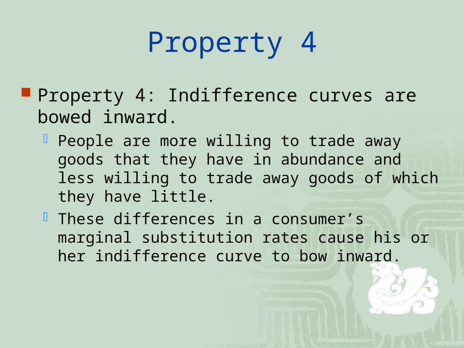
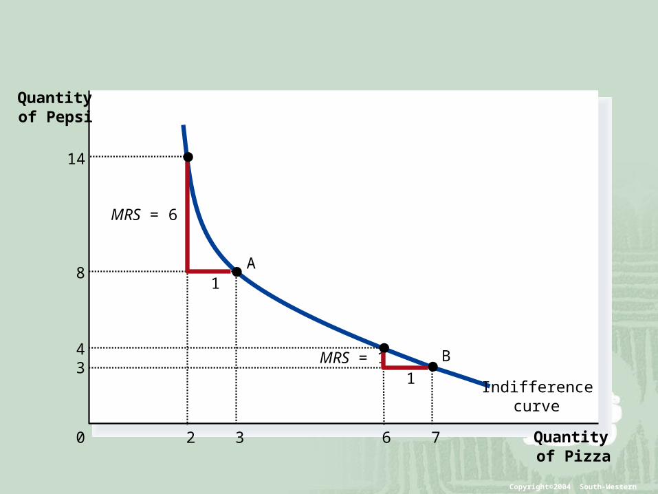
Property 4: Indifference curves are bowed inward. People are more willing to trade away goods that they

have in abundance and less willing to trade away goods of which they have little.

These differences in a consumer’s marginal substitution rates cause his or her indifference curve to bow inward.

Quantityof Pizza

Quantityof Pepsi

0

Indifferencecurve

8

3

A

3

7

B

1

MRS = 6

1MRS = 14

6

14

2


Two extreme Cases

Perfect Substitutes Two goods with straight-line indifference curves are

perfect substitutes. The marginal rate of substitution is a fixed number.

Perfect Complements Two goods with right-angle indifference curves are

perfect complements.

Dimes0

Nickels

(a) Perfect Substitutes

I1 I2 I3

3

6

2

4

1

2


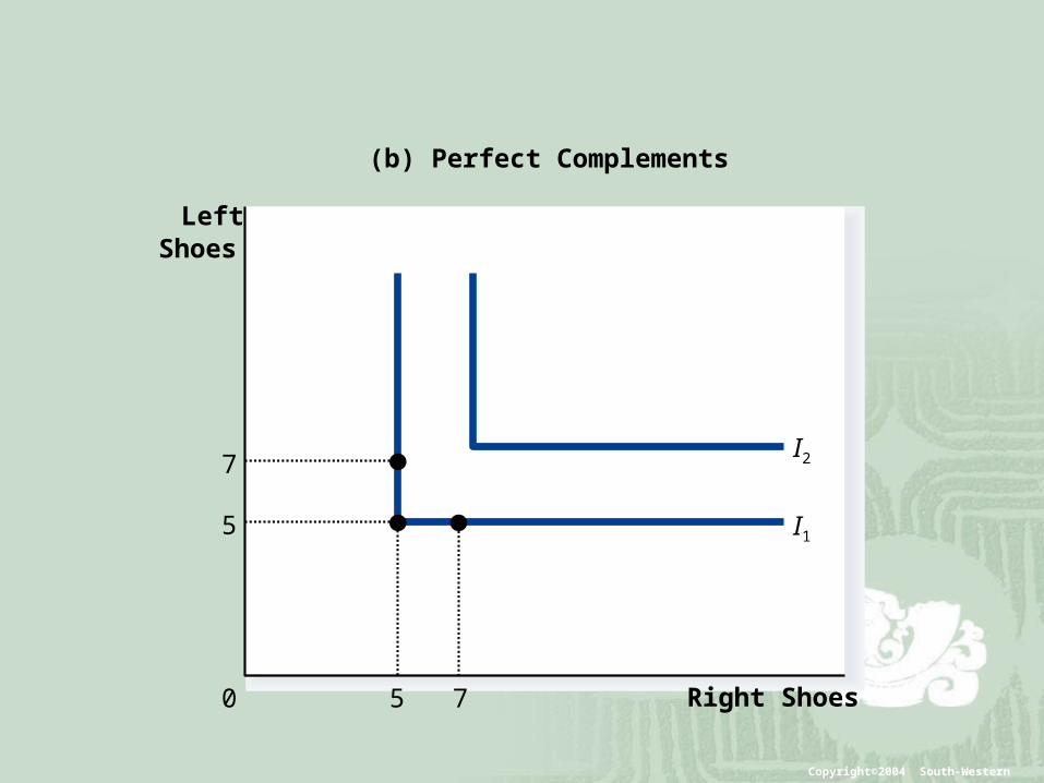
Right Shoes0

LeftShoes

(b) Perfect Complements

I1

I2

7

7

5

5


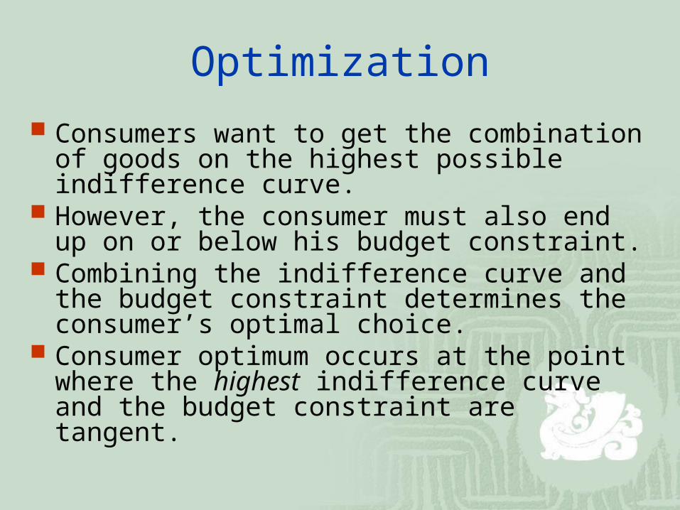
Optimization

Consumers want to get the combination of goods on the highest possible indifference curve.

However, the consumer must also end up on or below his budget constraint.

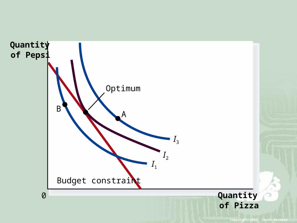
Combining the indifference curve and the budget constraint determines the consumer’s optimal choice.

Consumer optimum occurs at the point where the highest indifference curve and the budget constraint are tangent.

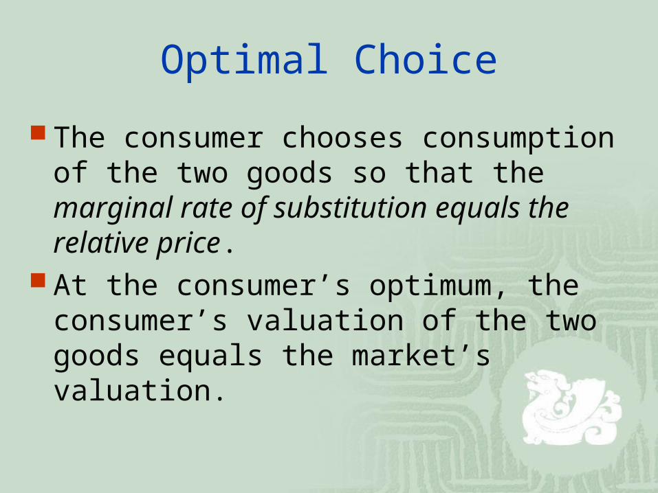
Optimal Choice

The consumer chooses consumption of the two goods so that the marginal rate of substitution equals the relative price.

At the consumer’s optimum, the consumer’s valuation of the two goods equals the market’s valuation.

Quantityof Pizza

Quantityof Pepsi

0

Budget constraint

I1

I2

I3

Optimum

AB


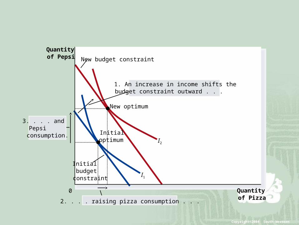
Income Changes

An increase in income shifts the budget constraint outward. The consumer is able to choose a better

combination of goods on a higher indifference curve.

Quantityof Pizza

Quantityof Pepsi

0

New budget constraint

I1

I2

2. . . . raising pizza consumption . . .

3. . . . andPepsiconsumption.

Initialbudgetconstraint

1. An increase in income shifts thebudget constraint outward . . .

Initialoptimum

New optimum


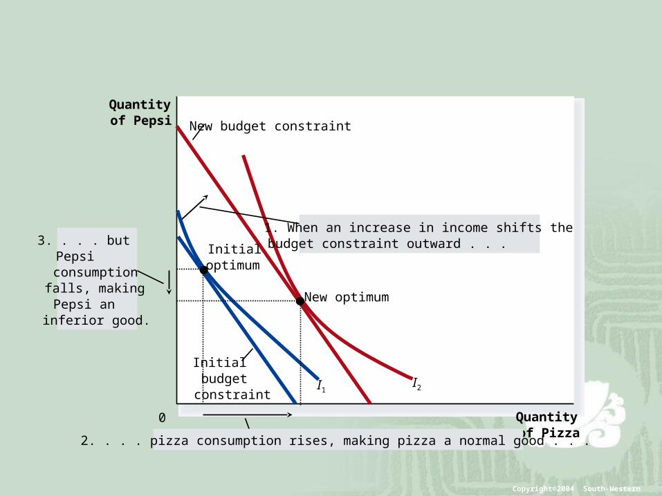
Normal versus Inferior

Normal versus Inferior Goods If a consumer buys more of a good when his or

her income rises, the good is called a normal good.

If a consumer buys less of a good when his or her income rises, the good is called an inferior good.

Quantityof Pizza

Quantityof Pepsi

0



I1I2

1. When an increase in income shifts thebudget constraint outward . . .3. . . . but

Pepsiconsumptionfalls, makingPepsi aninferior good.

2. . . . pizza consumption rises, making pizza a normal good . . .

Initialoptimum

New optimum


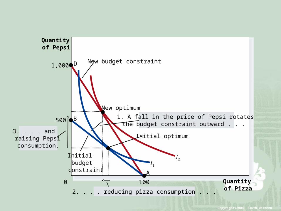
Price Changes

A fall in the price of any good rotates the budget constraint outward and changes the slope of the budget constraint.

Quantityof Pizza

Quantityof Pepsi

0

1,000 D

500 B

100

A

I1

I2

Initial optimum



1. A fall in the price of Pepsi rotates the budget constraint outward . . .

3. . . . andraising Pepsiconsumption.

2. . . . reducing pizza consumption . . .

New optimum


Price Effects

A price change has two effects on consumption. An income effect A substitution effect

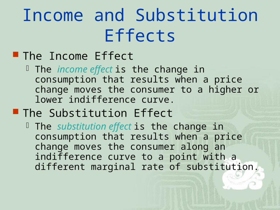
Income and Substitution Effects

The Income Effect The income effect is the change in consumption that

results when a price change moves the consumer to a higher or lower indifference curve.

The Substitution Effect The substitution effect is the change in consumption that

results when a price change moves the consumer along an indifference curve to a point with a different marginal rate of substitution.

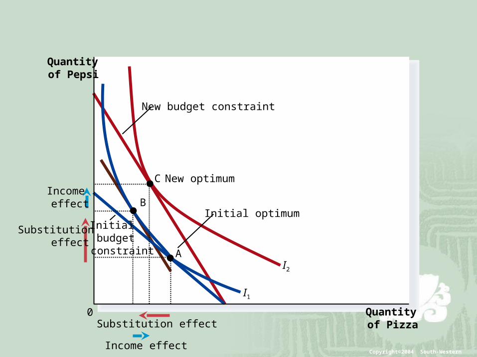
Income and Substitution Effects

A Change in Price: Substitution Effect A price change first causes the consumer to move from

one point on an indifference curve to another on the same curve.

Illustrated by movement from point A to point B.

A Change in Price: Income Effect After moving from one point to another on the same

curve, the consumer will move to another indifference curve.

Illustrated by movement from point B to point C.

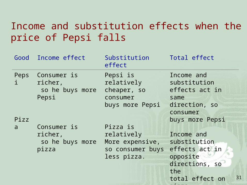
Income and substitution effects when the price of Pepsi falls

31

Good Income effect Substitution effect Total effect

Pepsi

Pizza

Consumer is richer, so he buys more Pepsi

Consumer is richer, so he buys more pizza

Pepsi is relativelycheaper, so consumerbuys more Pepsi

Pizza is relativelyMore expensive,so consumer buys less pizza.

Income and substitutioneffects act in samedirection, so consumerbuys more Pepsi

Income and substitutioneffects act in oppositedirections, so thetotal effect on pizzaconsumption isambiguous.

Quantityof Pizza

Quantityof Pepsi

0

I1

I2

A

Initial optimum



Substitutioneffect

Substitution effect

Incomeeffect

Income effect

B

C New optimum


Deriving Demand Curve

A consumer’s demand curve can be viewed as a summary of the optimal decisions that arise from his or her budget constraint and indifference curves.

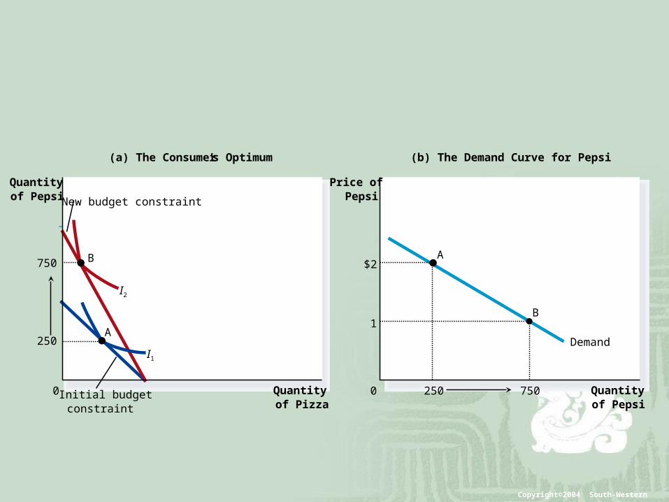
Quantityof Pizza

0

Demand

(a) The Consumer’s Optimum

Quantityof Pepsi

0

Price ofPepsi

(b) The Demand Curve for Pepsi

Quantityof Pepsi

250

$2A

750

1B

I1

I2


Initial budget constraint

750 B

250A


Giffen Goods

Do all demand curves slope downward? Demand curves can sometimes slope upward. This happens when a consumer buys more of a good

when its price rises. Giffen goods

Economists use the term Giffen good to describe a good that violates the law of demand.

Giffen goods are goods for which an increase in the price raises the quantity demanded.

The income effect dominates the substitution effect. They have demand curves that slope upwards.

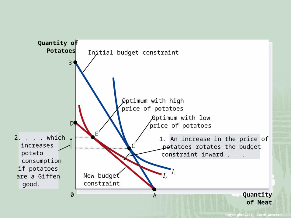
Quantityof Meat

Quantity ofPotatoes

0

I2

I1

Initial budget constraint

New budgetconstraint

D

A

B

2. . . . which increasespotatoconsumptionif potatoes

are a Giffengood.

Optimum with lowprice of potatoes

Optimum with highprice of potatoes

E

C1. An increase in the price ofpotatoes rotates the budgetconstraint inward . . .


Application 1

How do wages affect labor supply? Increase in wage

Budget constraint shifts outwardSteeperNew optimum

If enjoy more leisureWork lessBackward-sloping labor supply curveIncome effect dominates

An increase in the wage (a)

38

Consumption

(a) For a person with these preferences . . .

Hours of Leisure0

Wage

. . . the labor supply curve slopes upward.

Hours of LaborSupplied

0

Labor supply

I2

I1

BC2

BC1A

B

1. When the wage rises . . .

2. . . . hours of leisure decrease . . . 3. . . . and hours of labor increase

An increase in the wage (b)

39

Consumption

(b) For a person with these preferences . . .

Hours of Leisure0

Wage

. . . the labor supply curve slopes backward

Hours of LaborSupplied

0

Labor supplyI2

I1

BC2

BC1

1. When the wage rises . . .

2. . . . hours of leisure increase . . . 3. . . . and hours of labor decrease

Application 2

How do interest rates affect household saving?

Income decision Consume today or Save for future

Bundle of goods Consumption today and Consumption in the

future Relative price = interest rates Optimum: Budget constraint & Indifference

curves

The consumption-saving decision

41

Consumptionwhen Old

Consumptionwhen Young

0

I2

I1

I3

$110,000

100,000

Optimum

$50,000

55,000

Application 2: continued

Increase in interest rates Budget constraint – shifts outward

Steeper

Consumption in the future – rises If consume less today

Substitution effect dominates; Save more

If consume more todayIncome effect dominates; Save less

An increase in the interest rate

43

ConsumptionWhen

old

(a) Higher Interest Rate Raises Saving


0

I2

I1

BC2

BC1

1. A higher interest rate rotatesthe budget constraint outward . . .

ConsumptionWhen

old

(b) Higher Interest Rate Lowers Saving


0

I2

I1

BC2

BC1

2. . . . resulting in lower consumption when young and, thus, higher saving.

1. A higher interest rate rotatesthe budget constraint outward . . .

2. . . . resulting in higher consumption when young and, thus, lower saving.

Documents

Consumer Choice ETP Economics 101. Budget Constraint The budget constraint depicts the limit on the consumption “ bundles ” that a consumer can afford