Constructive Set Theory and Brouwerian Principles1

Michael Rathjen(Department of Mathematics, The Ohio State University,2

Email: rathjen@math.ohio-state.edu)

Abstract: The paper furnishes realizability models of constructive Zermelo-Fraenkelset theory, CZF, which also validate Brouwerian principles such as the axiom of con-tinuous choice (CC), the fan theorem (FT), and monotone bar induction (BIM), andthereby determines the proof-theoretic strength of CZF augmented by these principles.The upshot is that CZF+CC+FT possesses the same strength as CZF, or more pre-cisely, that CZF+CC+FT is conservative over CZF for Π0

2 statements of arithmetic,whereas the addition of a restricted version of bar induction to CZF (called decidablebar induction, BID) leads to greater proof-theoretic strength in that CZF+BID provesthe consistency of CZF.

Key Words: Constructive set theory, Brouwerian principles, partial combinatory al-gebra, realizability

Category: F.4.1

1 Introduction

Constructive Zermelo-Fraenkel Set Theory has emerged as a standard referencetheory that relates to constructive predicative mathematics as ZFC relates toclassical Cantorian mathematics. The general topic of Constructive Set Theoryoriginated in the seminal 1975 paper of John Myhill (cf. [16]), where a specific ax-iom system CST was introduced. Myhill developed constructive set theory withthe aim of isolating the principles underlying Bishop’s conception of what setsand functions are. Moreover, he wanted “these principles to be such as to makethe process of formalization completely trivial, as it is in the classical case” ([16],p. 347). Indeed, while he uses other primitives in his set theory CST besides thenotion of set, it can be viewed as a subsystem of ZF. The advantage of this is thatthe ideas, conventions and practise of the set theoretical presentation of ordi-nary mathematics can be used in the set theoretical development of constructivemathematics, too. Constructive Set Theory provides a standard set theoreticalframework for the development of constructive mathematics in the style of ErrettBishop and Douglas Bridges [6] and is one of several such frameworks for con-structive mathematics that have been considered. Aczel subsequently modifiedMyhill’s CST and the resulting theory was called Zermelo-Fraenkel set theory,CZF. A hallmark of this theory is that it possesses a type-theoretic interpre-tation (cf. [1, 2, 3]). Specifically, CZF has a scheme called Subset CollectionAxiom (which is a generalization of Myhill’s Exponentiation Axiom) whose for-malization was directly inspired by the type-theoretic interpretation.1 C. S. Calude, H. Ishihara (eds.). Constructivity, Computability, and Logic. A

Collection of Papers in Honour of the 60th Birthday of Douglas Bridges.2 This material is based upon work supported by the National Science Foundation

under Award No. DMS-0301162.

This paper studies augmentations of CZF by Brouwerian principles such asthe axiom of continuous choice (CC), the fan theorem (FT), and monotonebar induction (BIM). The objective is to determine whether these principlesincrease the proof-theoretic strength of CZF. More precisely, the research isconcerned with the question of whether any newΠ0

2 statements of arithmetic (i.e.statements of the form ∀n ∈ N ∃k ∈ NP (n, k) with P being primitive recursive)become provable upon adding CC, FT, and BIM (or any combination thereof)to the axioms of CZF.

The first main result obtained here is that CZF + CC + FT is indeed con-servative over CZF with respect to Π0

2 sentences of arithmetic. The first step inthe proof consists of defining a transfinite type structure over a special combi-natory algebra whose domain is the set of all arithmetical functions from N to Nwith application being continuous function application in the sense of Kleene’ssecond algebra K2. The transfinite type structure serves the same purpose as auniverse in Martin-Lof type theory. It gives rise to a realizability interpretationof CZF which also happens to validate the principles CC and FT. However, tobe able to show that FT is realized we have to employ classical reasoning in thebackground theory. It turns out that the whole construction can be carried outin a classical set theory known as Kripke-Platek set theory, KP. Since CZF andKP prove the same Π0

2 statements of arithmetic this establishes the result.A similar result can be obtained for CZF plus the so-called Regular Extension

Axiom, REA. Here it turns out that CZF+REA+CC+BIM isΠ02 conservative

over CZF+REA. This time the choice for the domain of the partial combinatoryalgebra is NN ∩ Lρ, where ρ = supn<ω ωckn with ωckn denoting the nth admissibleordinal. Application is again continuous function application. The transfinitetype structure also needs to be strengthened in that it has to be closed off underW -types as well. A background theory sufficient for these constructions is KPi,i.e. Kripke-Platek set theory plus an axiom asserting that every set is containedin an admissible set

The question that remains to be addressed is whether CZF + BIM is con-servative over CZF. This is answered in the negative in [25], where it is shownthat a restricted form of BIM - called decidable bar induction, BID - implies theconsistency of CZF on the basis of CZF. The proof makes use of results fromordinal-theoretic proof theory.

2 Constructive Zermelo-Fraenkel Set Theory

Constructive set theory grew out of Myhill’s endeavours (cf. [16]) to discovera simple formalism that relates to Bishop’s constructive mathematics as ZFCrelates to classical Cantorian mathematics. Later on Aczel modified Myhill’s settheory to a system which he called Constructive Zermelo-Fraenkel Set Theory,CZF.

Definition: 2.1 (Axioms of CZF) The language of CZF is the first order lan-guage of Zermelo-Fraenkel set theory, LST , with the non logical primitive symbol∈. CZF is based on intuitionistic predicate logic with equality. The set theoreticaxioms of axioms of CZF are the following:

1. Extensionality ∀a ∀b (∀y (y ∈ a ↔ y ∈ b) → a = b).

2. Pair ∀a ∀b∃x∀y (y ∈ x ↔ y = a ∨ y = b).3. Union ∀a∃x∀y (y ∈ x ↔ ∃z ∈ a y ∈ z).4. Restricted Separation scheme ∀a∃x∀y (y ∈ x ↔ y ∈ a ∧ ϕ(y)),

for every restricted formula ϕ(y), where a formula ϕ(x) is restricted, or ∆0,if all the quantifiers occurring in it are restricted, i.e. of the form ∀x∈ b or∃x∈ b.

5. Subset Collection scheme

∀a∀b∃c∀u(∀x∈ a∃y ∈ b ϕ(x, y, u) →

∃d∈ c (∀x∈ a ∃y ∈ d ϕ(x, y, u) ∧ ∀y ∈ d∃x∈ a ϕ(x, y, u)))

for every formula ϕ(x, y, u).6. Strong Collection scheme

∀a(∀x∈ a∃y ϕ(x, y) →

∃b (∀x∈ a ∃y ∈ b ϕ(x, y) ∧ ∀y ∈ b∃x∈ a ϕ(x, y)))

for every formula ϕ(x, y).7. Infinity

∃x∀u[u∈x ↔

(0 = u ∨ ∃v ∈x(u = v ∪ {v})

)]where y + 1 is y ∪ {y}, and 0 is the empty set, defined in the obvious way.

8. Set Induction scheme

(IND∈) ∀a (∀x∈ a ϕ(x) → ϕ(a)) → ∀a ϕ(a),

for every formula ϕ(a).

From Infinity, Set Induction, and Extensionality one can deduce that there existsexactly one set x such that ∀u

[u∈x ↔

(0 = u ∨ ∃v ∈x(u = v∪{v})

)]; this set

will be denoted by ω.

2.1 Choice principles

In many a text on constructive mathematics, axioms of countable choice anddependent choices are accepted as constructive principles. This is, for instance,the case in Bishop’s constructive mathematics (cf. [6] as well as Brouwer’s in-tuitionistic analysis (cf. [28], Chap. 4, Sect. 2). Myhill also incorporated theseaxioms in his constructive set theory [16].

The weakest constructive choice principle we shall consider is the Axiomof Countable Choice, ACω, i.e. whenever F is a function with domain ω suchthat ∀i∈ω ∃y ∈F (i), then there exists a function f with domain ω such that∀i∈ω f(i)∈F (i).

Let xRy stand for 〈x, y〉 ∈ R. A mathematically very useful axiom to havein set theory is the Dependent Choices Axiom, DC, i.e., for all sets a and (set)relations R ⊆ a× a, whenever

(∀x∈ a) (∃y ∈ a)xRy

and b0 ∈ a, then there exists a function f : ω → a such that f(0) = b0 and

(∀n∈ω) f(n)Rf(n+ 1).

Even more useful in constructive set theory is the Relativized DependentChoices Axiom, RDC. It asserts that for arbitrary formulae φ and ψ, whenever

∀x[φ(x) → ∃y

(φ(y) ∧ ψ(x, y)

)]and φ(b0), then there exists a function f with domain ω such that f(0) = b0 and

(∀n∈ω)[φ(f(n)) ∧ ψ(f(n), f(n+ 1))

].

One easily sees that RDC implies DC and DC implies ACω.

2.2 The strength of CZF

In what follows we shall use the notions of proof-theoretic equivalence of theoriesand proof-theoretic strength of a theory whose precise definitions one can find in[18]. For our purposes here we take proof-theoretic equivalence of set theories T1

and T2 to mean that these theories prove the same Π02 statements of arithmetic

and that this insight can be obtained on the basis of a weak theory such asprimitive recursive arithmetic, PRA.

Theorem: 2.2 Let KP be Kripke-Platek Set Theory (with the Infinity Axiom)(see [4]). The theory CZF bereft of Subset Collection is denoted by CZF−.

(i) CZF and CZF− are of the same proof-theoretic strength as KP and the clas-sical theory ID1 of non-iterated positive arithmetical inductive definitions.These systems prove the same Π0

2 statements of arithmetic.(ii) The system CZF augmented by the Power Set axiom is proof-theoretically

stronger than classical Zermelo Set theory, Z (in that it proves the consis-tency of Z).

(iii) CZF does not prove the Power Set axiom.

Proof: Let Pow denote the Power Set axiom. (i) follows from [17] Theorem4.14. Also (iii) follows from [17] Theorem 4.14 as one easily sees that 2-orderHeyting arithmetic has a model in CZF + Pow. Since second-order Heytingarithmetic is of the same strength as classical second-order arithmetic it fol-lows that CZF + Pow is stronger than classical second-order arithmetic (whichis much stronger than KP). But more than that can be shown. Working inCZF+Pow one can iterate the power set operation ω+ω times to arrive at theset Vω+ω which is readily seen to be a model of intuitionistic Zermelo Set Theory,Zi. As Z can be interpreted in Zi by means of a double negation translation aswas shown in [13] Theorem 2.3.2, we obtain (ii). 2

The first large set axiom proposed in the context of constructive set theorywas the Regular Extension Axiom, REA, which was introduced to accommodateinductive definitions in CZF (cf. [2], [3]).

Definition: 2.3 A set c is said to be regular if it is transitive, inhabited (i.e.∃u u ∈ c) and for any u∈ c and set R ⊆ u × c if ∀x∈u∃y 〈x, y〉 ∈R then thereis a set v ∈ c such that

∀x∈u∃y ∈ v 〈x, y〉 ∈R ∧ ∀y ∈ v ∃x∈u 〈x, y〉 ∈R.

We write Reg(a) for ‘a is regular’.REA is the principle

∀x∃y (x∈ y ∧ Reg(y)).

Theorem: 2.4 Let KPi be Kripke-Platek Set Theory plus an axiom assertingthat every set is contained in an admissible set (see [4]).

(i) CZF + REA is of the same proof-theoretic strength as KPi and the subsys-tem of second-order arithmetic with ∆1

2-comprehension and Bar Induction.(ii) CZF + REA does not prove the Power Set axiom.

Proof: (i) follows from [17] Theorem 5.13. (ii) is a consequence of (i) and The-orem 2.2. 2

3 Russian constructivism

We give a brief review of Russian constructivism which is intended to serve thepurpose of enhancing our account of Brouwerian intuitionism by contrast. Theconcept of algorithm or recursive function is fundamental to the Russian schoolsof Markov and Shanin. Contrary to Brouwer, this school takes the viewpointthat mathematical objects must be concrete, or at least have a constructivedescription, as a word in an alphabet, or equivalently, as an integer, for only onsuch objects do recursive functions operate. Furthermore, Markov adopts whathe calls Church’s thesis, CT, which asserts that whenever we see a quantifiercombination ∀n ∈ N ∃m ∈ NA(n,m), we can find a recursive function f whichproduces m from n, i.e. ∀n ∈ NA(n, f(n)). On the other hand, as far as purelogic is concerned he augments Brouwer’s intuitionistic logic by what is knownas Markov’s principle, MP, which may be expressed as

∀n ∈ N [A(n) ∨ ¬A(n)] ∧ ¬∀n ∈ N¬A(n) → ∃n ∈ NA(n),

with A containing natural number parameters only. The rationale for acceptingMP may be phrased as follows. Suppose A is a predicate of natural numberswhich can be decided for each number; and we also know by indirect argumentsthat there should be an n such that A(n). Then a computer with unboundedmemory could be programmed to search through N for a number n such thatA(n) and we should be convinced that it will eventually find one. As an examplefor an application of MP to the reals one obtains ∀x ∈ R (¬x ≤ 0 → x > 0).

In the next section we shall recall that Church’s thesis is incompatible withBrouwer’s principles CC and FTD.

CT is also incompatible with the axiom of choice AC1,0 to be defined inDefinition 4.1(2).

Lemma: 3.1 AC1,0 refutes CT.

Proof: See [27] or [5], Theorem 19.1. 2

One of the pathologies of CT is that it refutes the Uniform Continuity Principle(see Definition 4.13).

Theorem: 3.2 CT implies that there exists a continuous function f : [0, 1]→ Rwhich is unbounded and hence not uniformly continuous.

Proof: [28], 6.4.4. 2

However, in Russian constructivism one can also prove that all functions fromR to R are continuous. This requires a slight strengthening of CT.

Definition: 3.3 Extended Church’s Thesis, ECT, asserts that

∀n ∈ N[ψ(n)→ ∃m ∈ Nϕ(n,m)

]implies

∃e ∈ N ∀n ∈ N[ψ(n)→ ∃m, p ∈ N [T (e, n, p) ∧ U(p,m) ∧ ϕ(n,m)]

]whenever ψ(n) is an almost negative arithmetic formula and ϕ(u, v) is any for-mula. A formula θ of the language of CZF with quantifiers ranging over N issaid to be almost negative arithmetic if ∨ does not appear in it and instances of∃m ∈ N appear only as prefixed to primitive recursive subformulae of θ.

Note that ECT implies CT, taking ψ(n) to be n = n.

Theorem: 3.4 Under the assumptions ECT and MP, all functions f : R→ Rare continuous.

Proof: [28], 6.4.12. 2

4 Brouwer’s world

This section expounds on principles specific to Brouwer’s intuitionism and de-scribes their mathematical consequences.

Intuitionistic mathematics diverges from other types of constructive math-ematics in its interpretation of the term ‘sequence’. This led to the followingprinciple of continuous choice, abbreviated CC, which we divide into a con-tinuity part and a choice part:

Definition: 4.1 CC is the conjunction of (1) and (2):

1. Any function from NN to N is continuous.2. If P ⊆ NN×N, and for each α ∈ NN there exists n ∈ N such that (α, n) ∈ P ,

then there is a function f : NN → N such that (α, f(α)) ∈ P for all α ∈ NN.

The first part of CC will also be denoted by Cont(NN,N). The second part ofCC is often denoted by AC1,0.

The justification for CC springs from Brouwer’s ideas about choice sequences.Let P ⊆ NN × N, and suppose that for each α ∈ NN there exists n ∈ N suchthat (α, n) ∈ P . According to Brouwer, the construction of an element of NN isforever incomplete. A generic sequence α is purely extensional, in the sense thatat any given moment we can know nothing about α other than a finite numberof its terms. It follows that for a given sequence α, our procedure for findingan n ∈ N such that (α, n) ∈ P must be able to calculate n from some finite

initial sequence α(m).3 If β is another such sequence, and α(m) = β(m), thenour procedure must return the same n for β as it does for α. So this proceduredefines a continuous function f : NN → N such that (α, f(α)) ∈ P for all α ∈ NN.

It is plain that Cont(NN,N) is incompatible with classical logic.

The other principle central to Brouwerian mathematics is the so-called FanTheorem which is also classically valid and equivalent to Konig’s lemma, KL.

Definition: 4.2 Let 2N be the set of all binary sequences α : N → {0, 1} andlet 2∗ be the set of finite sequences of 0s and 1s. For s, t ∈ 2∗ we write s ⊆ t tomean that s is an initial segment of t. A bar of 2∗ is subset R of 2∗ such thatthe following property holds:

∀α ∈ 2N ∃n α(n) ∈ R.The bar R is decidable if it also satisfies

∀s ∈ 2∗ (s ∈ R ∨ s /∈ R).

FTD is the statement that every decidable bar R of 2∗ is uniform, i.e., thereexists a natural number m such that

∀α ∈ 2N ∃k ≤ m α(k) ∈ R.The Fan Theorem or General Fan Theorem, FT, is the statement that every barR of 2∗ is uniform.

Lemma: 4.3 FTD refutes CT.

Proof: Apply FTD to Kleene’s singular tree. For details see [28] 4.7.6. 2

4.1 Decidable Bar induction

Brouwer justified FTD by appealing to a principle known as decidable BarInduction, BID.

Definition: 4.4 Let N∗ be the set of all finite sequences of natural numbers.If s ∈ N∗, m ∈ N and s = 〈s0, . . . sk〉 then s ∗ 〈m〉 denotes the sequence〈s0, . . . , sk,m〉. A bar of N∗ is defined in the same vein as a bar of 2∗.

BID is asserts that for every decidable bar R of N∗ and arbitrary class Q,

∀s ∈ N∗ (s ∈ R→ s ∈ Q) ∧∀s ∈ N∗ [(∀k ∈ N s ∗ 〈k〉 ∈ Q)→ s ∈ Q] →〈〉 ∈ Q.

Monotone Bar Induction, BIM, asserts that for every bar R of N∗ and arbitraryclass Q,

∀s, t ∈ N∗ (s ∈ R→ s ∗ t ∈ R) ∧∀s ∈ N∗ (s ∈ R→ s ∈ Q) ∧∀s ∈ N∗ [(∀k ∈ N s ∗ 〈k〉 ∈ Q)→ s ∈ Q) →〈〉 ∈ Q.

It is easy to see that BIM entails BID (cf. [10], Theorem 3.7).3 α(0) := 〈〉, α(k + 1) = 〈α(0), . . . , α(k)〉.

Corollary: 4.5 BID implies FTD and BIM implies FT.

Proof: See [15], Ch.I,§6.10 (or exercise). 2

4.2 Local continuity

In connection with Brouwer’s intuitionism, one often works with the local con-tinuity, LCP, rather than CC. LCP entails Cont(NN,N) but not AC1,0.

Definition: 4.6 For α, β ∈ NN we write β ∈ α(n) to mean β(n) = α(n).The Local Continuity Principle, LCP, states that

∀α ∈ NN ∃n ∈ NA(α, n)→∀α ∈ NN ∃n,m ∈ N ∀β ∈ NN [β ∈ α(m)→ A(β, n)].

LCP is also known as the Weak Continuity Principle (WC-N) (see [28], p.371) or Brouwer’s Principle for Numbers (BP0).

Some obvious deductive relationships between some of the principles are recordedin the next lemma.

Lemma: 4.7 (i) LCP⇒ Cont(NN,N).(ii) CC⇔ LCP ∧ AC1,0

Proof: Obvious. 2

While CC entails the choice principle AC1,0, it is not compatible with choicefor higher type objects. In point of fact, the incompatibility already occurs inconnection with a consequence of CC.

Lemma: 4.8 Let AC2,0 be the following principle:

If P is a subset of (NN → N) × N such that for every f : NN → Nthere exists n ∈ N such that (f, n) ∈ P , then there exists a functionF : (NN → N)→ N such that for all f : NN → N, (f, F (f)) ∈ P .

AC2,0 refutes Cont(NN,N).

Proof: See [27] or [5], Theorem 19.1. 2

LCP and a fortiori CC refute principles of omniscience. For α ∈ 2N letαn := α(n).

Definition: 4.9 Limited Principle of Omniscience (LPO):

∀α ∈ 2N [∃nαn = 1 ∨ ∀nαn = 0].

Lesser Limited Principle of Omniscience (LLPO):

∀α ∈ 2N (∀n,m[αn = αm = 1→ n = m] → [∀nα2n = 0 ∨ ∀nα2n+1 = 0]).

Lemma: 4.10 (i) LCP⇒ ¬LPO.(ii) CC⇒ ¬LLPO.

Proof: (i) follows from [28] 4.6.4. (ii) is proved in [7], 5.2.1. 2

LCP is also incompatible with Church’s thesis.

Lemma: 4.11 LCP implies ¬CT.

Proof: [28], 4.6.7. Apply LCP to CT. 2

With the help of LCP one deduces Brouwer’s famous theorem.

Theorem: 4.12 If LCP holds, then every map f : R→ R is pointwise contin-uous.

Proof: [28] Theorem 6.3.4. 2

Definition: 4.13 Brouwer needed the fan theorem to derive the classically validUniform Continuity Principle:

UC Every pointwise continuous function from 2N to Nis uniformly continuous.

Lemma: 4.14 FT implies UC.

Proof: [28] Theorem 6.3.6. 2

Under LCP we can drop the condition of continuity.

Corollary: 4.15 If LCP and FT hold, then every f : [a, b] → R is uniformlycontinuous and has a supremum.

Proof: [28] Theorem 6.3.8. 2

Theorem: 4.16 Under the hypothesis CC, the statements UC and FTD areequivalent.

Proof. See [7] Theorem 5.3.2 and Corollary 5.3.4. 2

Corollary: 4.17 If CC and FTD hold, then every mapping of a nonvoid com-pact metric space into a metric space is uniformly continuous.

Proof: [7], Theorem 5.3.6. 2

5 More Continuity Principle

Another continuity principle one finds in the literature is Strong Continuityfor Numbers:

C-N ∀α ∈ NN ∃n ∈ N A(α, n) → ∃γ ∈ K∗ ∀α ∈ NN A(α, γ(α)), (1)

where K∗ is the class of neighbourhood functions, i.e. γ ∈ K∗ iff γ : N∗ → N,γ(〈〉) = 0, and

∀s, t ∈ N∗ [γ(s) 6= 0→ γ(s) = γ(s ∗ t)] ∧ ∀α ∈ NN ∃n ∈ N γ(α(n)) 6= 0,

andγ(α) = n iff ∃m ∈ N [γ(α(m)) = n+ 1].

Dummett in [10], p. 60 refers to C-N as ‘the Continuity Principle’ and assignsit the acronym CP∃n.

In point of fact, C-N is just a different rendering of CC.

A yet stronger continuity principle is functional continuous choice F-CC orCONT1 (cf. [28],7.6.15) (also denoted by C-C in [28],7.6.15 and by CP∃β in [10],p. 60):

F-CC ∀α ∈ NN∃β ∈ NN A(α, β)→ ∃γ ∈ K∗ ∀α ∈ NN A(α, γ|α).

F-CC is not considered to be part of Brouwer’s realm as it is actually inconsistentwith some of Brouwer’s later, though controversial, proposals about the “creativesubject” (see [10] 6.3).

In point of fact, F-CC is equivalent to the schema

F-CC′ ∀α ∈ NN∃β ∈ NN A(α, β)→ ∃γ ∈ NN ∀α ∈ NN A(α, γ|α).

Lemma: 5.1 (i) C-N ⇔ CC.(ii) F-CC implies CC.

Proof: For (i) see [7], p. 119. (ii) is to be found in [28], 7.6.15. 2

In the presence of CC, one can actually dispense with the decidability of thebar in FTD and BID.

Lemma: 5.2 Assuming CC, FTD implies FT and BID implies BIM.

Proof: This follows from C-N ⇔ CC by [10], Theorem 3.8 and the proof ofthe general fan theorem of [10], page 64. 2

6 Elementary analysis augmented by Brouwerian principles

Realizability interpretations of Brouwerian principles have been given for elemen-tary analysis. It should be instructive to review these results before venturing tothe more complex realizability models required for set theory.

Elementary analysis, EL, is a two-sorted intuitionistic formal system withvariables x, y, z, . . . and α, β, γ, . . . intended to range over natural numbers andvariables intended to range over one-place total functions from N to N, respec-tively. The language of EL is an extension of the language of of Heyting Arith-metic. In particular, π is a symbol for a primitive-recursive pairing function onN× N and S is the symbol for the successor function.

EL is a conservative extension of Heyting Arithmetic. The details of thistheory are described in [15] Ch.I and [28], Ch.3,Sect.6. There is λ-abstractionfor explicit definitions of functions, and a recursion-operator Rec such that (t anumerical term, φ a function term; φ(t, t′) := φ(π(t, t′)))

Rec(t, φ)(0) = t, Rec(t, φ)(Sx) = φ(x,Rec(t, φ)(x)).

Induction is extended to all formulas in the new language. The functions of ELare assumed to be closed under “recursive in”, which is expressed by includinga weak choice axiom for quantifier-free A:

QF-AC ∀x∃y A(x, y)→ ∃α∀xA(x, α(x)).

Definition: 6.1 In EL we introduce abbreviations for partial continuous appli-cation:

α(β) = x := ∃y[α(β(y)) = x+ 1 ∧ ∀y′ < y (α(β(y′)) = 0

],

α|β = γ := ∀x[λn.α(〈x〉 ∗ n)(β) = γ(x)] ∧ α(0) = 0.

We may introduce |,·(·) as primitive operators in a conservative extension EL∗

based on the logic of partial terms.

It was shown by Kleene in [15],Ch.II that EL augmented by the principles BIMand C-N is consistent. For this purpose he used a realizability interpretationbased on continuous function application, i.e. the second Kleene algebra K2.As this paper will follow a similar strategy for gauging the strength of CZFextended by Brouwerian principles it is instructive to review Kleene’s results.

Definition: 6.2 (Function realizability) In EL equality of functions α = βis not a prime formula and defined by ∀xα(x) = β(x).

α|β ↓ stands for ∃γ α|β = γ.The function realizability interpretation is an inductively defined translation

of a formula A of EL into a formula α rf A of EL, where α is a fresh variablenot occurring in A:

α rf ⊥ iff ⊥α rf t = s iff t = sα rf A ∧B iff π0α rf A ∧ π1α rf Bα rf A ∨B iff [α(0) = 0→ α+ rf A] ∧ [α(0) 6= 0→ α+ rf B]α rf A→ B iff ∀β [β rf A→ α|β ↓ ∧α|β rf B]α rf ∀xA(x) iff ∀x [α|λn.x ↓ ∧ α|λn.x rf A(x)]α rf ∃xA(x) iff α+ rf A(α(0))α rf ∀βA(β) iff ∀β [α|β ↓ ∧α|β rf A(β)]α rf ∃βA(β) iff π1α rf A(π0α)

with π0, π1 being the projection functions with respect to some fixed primitiverecursive pairing function π : N × N → N and α+ being the tail of α (i.e.α = 〈α0〉 ∗ α+).

Lemma: 6.3 Let A be a closed formula of EL. If EL + C-N ` A, then EL `∃α rf A.

Proof: See [26], theorem 3.3.11. 2

Kleene shows in [15], Ch.11, Lemma 9.10 that the arithmetical functionsconstitute the least class of functions C ⊆ NN closed under general recursivenessand the jump operation ’ (look there for precise definitions).

An inhabited set C ⊆ NN gives rise to a structure NC for the language of ELas follows: The domain of NC is N ∪ C, the number variables range over N; thefunction variables range over C, and the other primitives of EL are interpretedin the standard way.

Lemma: 6.4 (KP) For any set of functions C ⊆ NN closed under general re-cursiveness and the jump operation ’: the fan theorem FT holds in the classicalmodel NC of EL, when the representing function of the bar R belongs to C.

Proof: [15], Lemma 9.12. 2

Theorem: 6.5 (KP) For any set of functions C ⊆ NN closed under generalrecursiveness and the jump operation ’ (e.g. the arithmetical functions): If EL+C-N + FT ` A, then NC |= ∃αα rf A.

Proof: [15], Ch.11 Theorem 9.13. 2

Kleene’s proof of Theorem 6.5 can actually be extended to include BIM.

Definition: 6.6 An inhabited set of functions C ⊆ NN is said to be a β-modelif C is closed under general recursiveness and the jump operation ’ and whenever≺ is a binary relation on N whose representing function is in C and NC |=∀α∃n¬α(n+ 1) ≺ α(n), then ≺ is well-founded.

Lemma: 6.7 (KPi) If C ⊆ NN is a β-model then monotone bar induction holdsin the classical model NC of EL, when the representing function of the bar Rbelongs to C.

Proof: Similar to [15], Ch.11 Lemma 9.12. 2

Theorem: 6.8 (KPi) For any β-model C ⊆ NN (e.g. the functions in NN ∩ Lρ,where ρ = supn<ω ωckn with ωckn being the nth admissible ordinal; cf. [4]):

If EL + C-N + BIM ` A, then NC |= ∃αα rf A.

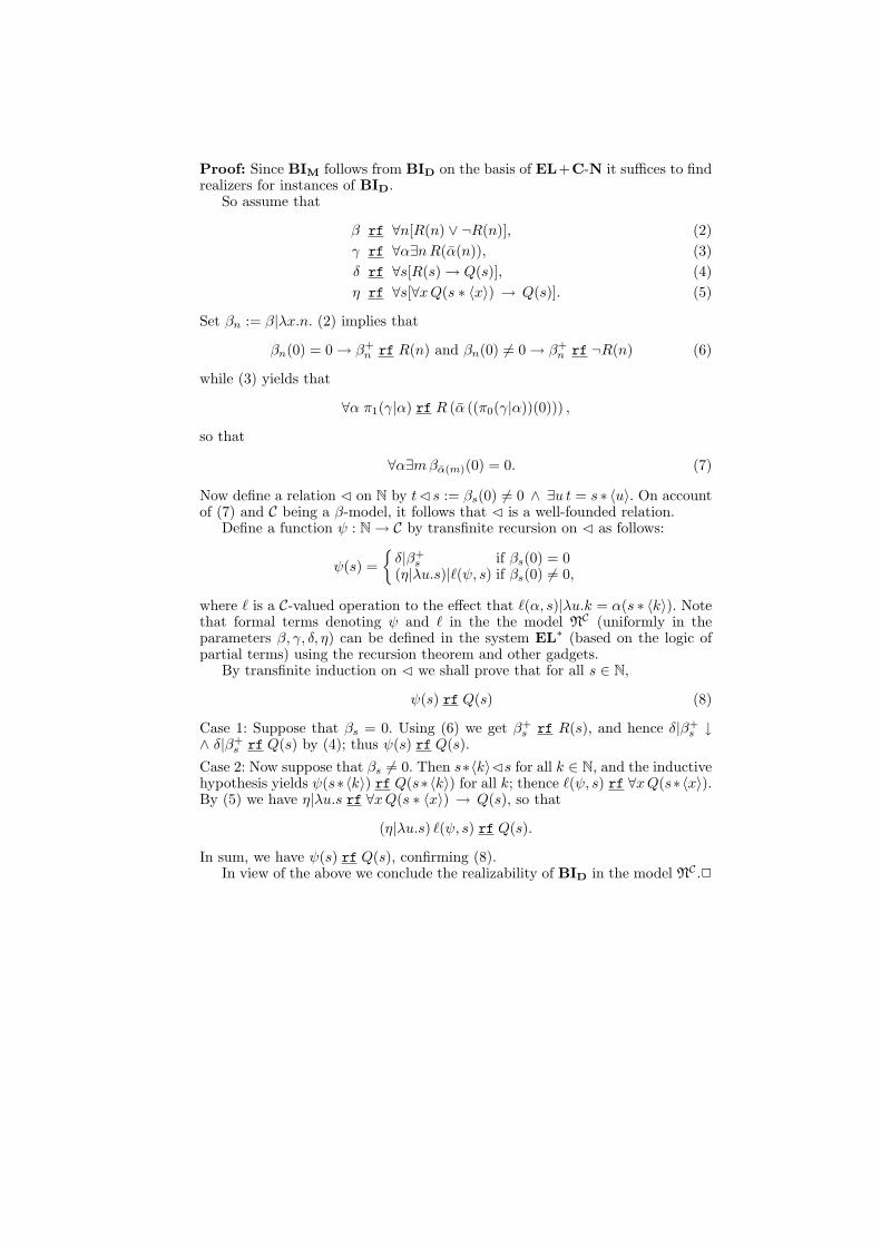
Proof: Since BIM follows from BID on the basis of EL+C-N it suffices to findrealizers for instances of BID.

So assume that

β rf ∀n[R(n) ∨ ¬R(n)], (2)γ rf ∀α∃nR(α(n)), (3)δ rf ∀s[R(s)→ Q(s)], (4)η rf ∀s[∀xQ(s ∗ 〈x〉) → Q(s)]. (5)

Set βn := β|λx.n. (2) implies that

βn(0) = 0→ β+n rf R(n) and βn(0) 6= 0→ β+

n rf ¬R(n) (6)

while (3) yields that

∀α π1(γ|α) rf R (α ((π0(γ|α))(0))) ,

so that

∀α∃mβα(m)(0) = 0. (7)

Now define a relation � on N by t� s := βs(0) 6= 0 ∧ ∃u t = s ∗ 〈u〉. On accountof (7) and C being a β-model, it follows that � is a well-founded relation.

Define a function ψ : N→ C by transfinite recursion on � as follows:

ψ(s) ={δ|β+

s if βs(0) = 0(η|λu.s)|`(ψ, s) if βs(0) 6= 0,

where ` is a C-valued operation to the effect that `(α, s)|λu.k = α(s ∗ 〈k〉). Notethat formal terms denoting ψ and ` in the the model NC (uniformly in theparameters β, γ, δ, η) can be defined in the system EL∗ (based on the logic ofpartial terms) using the recursion theorem and other gadgets.

By transfinite induction on � we shall prove that for all s ∈ N,

ψ(s) rf Q(s) (8)

Case 1: Suppose that βs = 0. Using (6) we get β+s rf R(s), and hence δ|β+

s ↓∧ δ|β+

s rf Q(s) by (4); thus ψ(s) rf Q(s).

Case 2: Now suppose that βs 6= 0. Then s∗〈k〉�s for all k ∈ N, and the inductivehypothesis yields ψ(s∗〈k〉) rf Q(s∗〈k〉) for all k; thence `(ψ, s) rf ∀xQ(s∗〈x〉).By (5) we have η|λu.s rf ∀xQ(s ∗ 〈x〉) → Q(s), so that

(η|λu.s) `(ψ, s) rf Q(s).

In sum, we have ψ(s) rf Q(s), confirming (8).In view of the above we conclude the realizability of BID in the model NC .2

7 Combinatory Algebras

The meaning of the logical operations in intuitionistic logic is usually explainedvia the so-called Brouwer-Heyting-Kolmogorov-interpretation (commonly abbre-viated to BHK-interpretation; for details see [28], 1.3.1). The notion of functionis crucial to any concrete BHK-interpretation in that it will determine the settheoretic and mathematical principles validated by it. The most important se-mantics for intuitionistic theories, known as realizability interpretations, alsorequire that we have a set of (partial) functions on hand that serve as realizersfor the formulae of the theory. An abstract and therefore “cleaner” approachto this semantics considers realizability over general domains of computationsallowing for recursion and self-application. These structures have been variablycalled partial combinatory algebras, applicative structures, or Schonfinkel alge-bras. They are closely related to models of the λ-calculus.

Let (M, ·) be a structure equipped with a partial operation, that is, · is a binaryfunction with domain a subset of M ×M and co-domain M . We often omit thesign “·” and adopt the convention of “association to the left”. Thus exy means(e ·x) ·y. We also sometimes write e ·x in functional notation as e(x). Extendingthis notion to several variables, we write e(x, y) for exy etc.

Definition: 7.1 A PCA is a structure (M, ·), where · is a partial binary opera-tion on M , such that M has at least two elements and there are elements k ands in M such that kxy and sxy are always defined, and

(i) kxy = x(ii) sxyz ' xz(yz),

where ' means that the left hand side is defined iff the right hand side is defined,and if one side is defined then both sides yield the same result.

(M, ·) is a total PCA if a · b is defined for all a, b ∈M .

Definition: 7.2 Partial combinatory algebras are best described as the modelsof a formal theory PCA. The language of PCA has two distinguished constantsk and s. To accommodate the partial operation in a standard first order language,the language of PCA has a ternary relation symbol Ap. The terms of PCA arejust the variables and constants. Ap will almost never appear in what follows aswe prefer to write t1t2 ' t3 for Ap(t1, t2, t3). In order to facilitate the formulationof the axioms, the language of PCA is expanded definitionally with the symbol' and the auxiliary notion of an application term or partial term is introduced.The set of application terms is given by two clauses:

1. All terms of PCA are application terms; and2. If s and t are application terms, then (st) is an application term.

For s and t application terms, we have auxiliary, defined formulae of the form:

s ' t := ∀y(s ' y ↔ t ' y),

if t is not a variable. Here s ' a (for a a free variable) is inductively defined by:

s ' a is

{s = a, if s is a term of PCA,∃x, y[s1 ' x ∧ s2 ' y ∧ Ap(x, y, a)] if s is of the form (s1s2).

Some abbreviations are t1t2 . . . tn for ((...(t1t2)...)tn); t ↓ for ∃y(t ' y) and φ(t)for ∃y(t ' y ∧ φ(y)).

In this paper, the logic of PCA is assumed to be that of intuitionisticpredicate logic with identity. PCA’s non-logical axioms are the following:

Axioms of PCA

1. ab ' c1 ∧ ab ' c2 → c1 = c2.2. (kab) ↓ ∧ kab ' a.3. (sab) ↓ ∧ sabc ' ac(bc).

The following shows how λ-terms can be constructed in PCA.

Lemma: 7.3 For each application term t and variable x, one can construct aterm λx.t, whose free variables are those of t, excluding x, such that PCA `λx.t ↓ and PCA ` (λx.t)u ' t[x/u] for all application terms u, where t[x/u]results from t by replacing x in t throughout by u.

Proof: We proceed by induction on the buildup of t. (i) λx.x is skk; (ii) λx.t is ktfor t a constant of PCA or variable other than x; (iii) λx.t1t2 is s(λx.t1)(λx.t2).2

Having λ-terms on hand, one can easily prove the recursion or fixed pointtheorem in PCA, and consequently that all recursive functions are definablein PCA. The elegance of the combinators arises from the fact that, at least intheory, anything that can be done in a programming language can be done usingsolely k and s.

Lemma: 7.4 (Recursion Theorem) There is an application term r such thatPCA proves:

rx ↓ ∧ rxy ' x(rx)y.

Proof: Let r be λx.gg with g := λzy.x(zz)y. Then rx ' gg ' (λzy.x(zz)y)g' λy.x(gg)y, so that rx ↓ by Lemma 7.3. Moreover, rxy ' x(gg)y ' x(rx)y. 2

Corollary: 7.5 PCA ` ∀f∃g∀x1 . . . ∀xn g(x1, . . . , xn) ' f(g, x1, . . . , xn).

It often convenient to equip a PCA with additional structure such as pairing,natural numbers, and some form of definition by cases. In fact, these gadgetscan be constructed in any PCA, as Curry showed. Nonetheless, it is desirable toconsider richer structures as the natural models for PCAs we are going to studycome already furnished with a “natural” copy of the natural numbers, naturalpairing functions, etc., which are different from the constructions of combinatorylogic.

Definition: 7.6 The language of PCA+ is that of PCA, with a unary rela-tion symbol N (for a copy of the natural numbers) and additional constants0, sN ,pN ,d,p,p0,p1 for, respectively, zero, successor on N , predecessor on N ,definition by cases on N , pairing, and the corresponding two projections.

The axioms of PCA+ are those of PCA, augmented by the following:

1. (pa0a1) ↓ ∧ (p0a) ↓ ∧ (p1a) ↓ ∧ pi(pa0a1) ' ai for i = 0, 1.2. N(c1) ∧ N(c2) ∧ c1 = c2 → dabc1c2 ↓ ∧ dabc1c2 ' a.3. N(c1) ∧ N(c2) ∧ c1 6= c2 → dabc1c2 ↓ ∧ dabc1c2 ' b.4. ∀x

(N(x)→

[sNx ↓ ∧ sNx 6= 0 ∧ N(sNx)

]).

5. N(0) ∧ ∀x(N(x) ∧ x 6= 0→

[pNx ↓ ∧ sN (pNx) = x

]).

6. ∀x[N(x)→ pN (sNx) = x

].

The extension of PCA+ by the schema of induction for all formulae,

ϕ(0) ∧ ∀x[N(x) ∧ ϕ(x)→ ϕ(sNx)

]→ ∀x

[N(x)→ ϕ(x)

]is is known by the acronym EON (elementary theory of operations and numbers)or APP (applicative theory). For full details about PCA, PCA+, and EONsee [11, 12, 5, 28].

Let 1 := sN 0. The applicative axioms entail that 1 is an application term thatevaluates to an object falling under N but distinct from 0, i.e., 1 ↓, N(1) and0 6= 1. More generally, we define the standard integers of a PCA to be theinterpretations of the numerals, i.e. the terms n defined by 0 = 0 and n+ 1 =sN n for n ∈ N. Note that PCA+ ` n ↓.

A PCA+ (M, ·, . . .) whose integers are standard, meaning that {x ∈M |M |=N(x)} is the set consisting of the interpretations of the numerals in M , will becalled an ω-PCA+. Note that an ω-PCA+ is also a model of APP.

Some further conventions are useful. Systematic notation for n-tuples is in-troduced as follows: (t) is t, (s, t) is pst, and (t1, . . . , tn) is defined by((t1, . . . , tn−1), tn).

Lemma: 7.7 PCA+ is conservative over PCA.

Proof: See [5],VI,2.9. 2

7.1 Kleene’s Examples of Combinatory Algebras

The primordial PCA is furnished by Turing machine application on the integers.There are many other interesting PCAs that provide us with a laboratory forthe study of computability theory. As the various definitions are lifted to moregeneral domains and notions of application other than Turing machine applica-tions some of the familiar results break down. By studying the notions in thegeneral setting one sees with a clearer eye the truths behind the results on theintegers.

7.1.1 Kleene’s first model

The “standard” applicative structure is Kleene’s first model, called K1, in whichthe universe |K1| is N and ApK1(x, y, z) is Turing machine application:

ApK1(x, y, z) iff {x}(y) ' z.

The primitive constants of PCA+ are interpreted over N in the obvious way,and N is interpreted as N.

Kleene’s second model

The universe of “Kleene’s second model” of APP, K2, is NN. The most interest-ing feature of K2 is that in the type structure over K2, every type-2 functionalis continuous.

We shall use α, β, γ, . . . as variables ranging over functions from N to N. Inorder to describe this PCA, it will be necessary to review some terminology.

Definition: 7.8 We assume that every integer codes a finite sequence of inte-gers. For finite sequences σ and τ , σ ⊂ τ means that σ is an initial segmentof τ ; σ ∗ τ is concatenation of sequences; 〈〉 is the empty sequence; 〈n0, . . . , nk〉displays the elements of a sequence; if this sequence is τ then lh(τ) = k+1 (read“length of τ”); α(m) = 〈α(0), . . . , α(m − 1)〉 if m > 0; α(0) = 〈〉. A function αand an integer n produce a new function 〈n〉 ∗ α which is the function β withβ(0) = n and β(k + 1) = α(k).

Application requires the following operations on NN:

α � β = m iff ∃n [α(βn) = m+ 1 ∧ ∀i < nα(βi) = 0](α|β)(n) = α � (〈n〉 ∗ β)

We would like to define application on NN by α|β, but this is in general only apartial function, therefore we set:

α · β = γ iff ∀n (α|β)(n) = γ(n). (9)

Theorem: 7.9 K2 is a model of APP.

Proof: For the natural numbers of K2 take N := {n|n ∈ N}, where n de-notes the constant function on N with value n. For pairing define the functionP : NN → NN by P (α, β)(n) = α(n/2) if n is even and P (α, β)(n) = β(n−1

2 ) ifn is odd. We then have to find a specific π ∈ NN such that (π|α)|β = P (α, β)for all α and β. Details on how to define all the constants of APP in K2 can befound in [28],Ch.9,Sect.4. 2

Substructures of Kleene’s second model

Inspection of the definition of application in K2 shows that subcollections ofNN closed under “recursive in” give rise to substructures of K2 that are modelsof APP as well. Specifically, the set of unary recursive functions forms a sub-structure of K2 as does the set of arithmetical functions from N to N, i.e., thefunctions definable in the standard model of Peano Arithmetic, furnish a modelof APP when equipped with the application of (9).

8 Type Structures over Combinatory Algebras

We shall define an “internal” version of a transfinite type structure with depen-dent products and dependent sums over any applicative structure.

Definition: 8.1 Let P = (P, ·, . . .) be an ω-PCA+. The types of P and theirelements are defined inductively. The set of elements of a type A is called itsextension and denoted by A. The type structure will be denoted by T P.

1. NPis a type with extension the set of integers of P, i.e., {x ∈ P |P |= N(x)}.

2. For each integer n, NP

n is a type with extension {kP | k = 0, . . . n− 1} if n > 0and NP

0 = ∅.3. U

Pis a type with extension P .

4. If A and B are types, then A+P B is a type with extension

{(0, x) |x ∈ A} ∪ {(1, x) |x ∈ B}.

5. If A is a type and for each x ∈ A, F (x) is a type, where F ∈ P and F (x)means F · x, then

P∏x:A

F (x)

is a type with extension {f ∈ P | ∀x ∈ A f · x ∈ F (x)}.6. If A is a type and for each x ∈ A, F (x) is a type, where F ∈ P , then

P∑x:A

F (x)

is a type with extension {(x, u) |x ∈ A ∧ u ∈ F (x)}.

The obvious question to ask is: Why should we distinguish between a type Aand its extension A. Well, the reason is that we want to apply the applicationoperation of P to types. For this to be possible, types have to be elements of P .Thus types aren’t sets. Alternatively, however, we could identify types with setsand require that they be representable in P in some way. This can be arrangedby associating Godel numbers in P with types and operations on types. This iseasily achieved by employing the coding facilities of the PCA+ P. For instance,if the types A and B have Godel numbers pAq and pBq, respectively, thenA + B has Godel number (1, pAq, pBq), and if C is a type with Godel numberpCq, F ∈ P , and for all x ∈ C, F (x) is the Godel number of a type Bx, then(2, pCq, F ) is the Godel number of the dependent type

∏P

x:C Bx, etc. In whatfollows we will just identify types with their extensions (or their codes) as suchontological distinctions are always retrievable from the context.

Remark: 8.2 The ordinary product and arrow types can be defined with theaid of dependent products and sums, respectively. Let A,B be types and F ∈ Pbe a function such that F (x) = B for all x ∈ P .

A×B :=

P∑x:A

F (x) A→ B :=

P∏x:A

F (x).

.

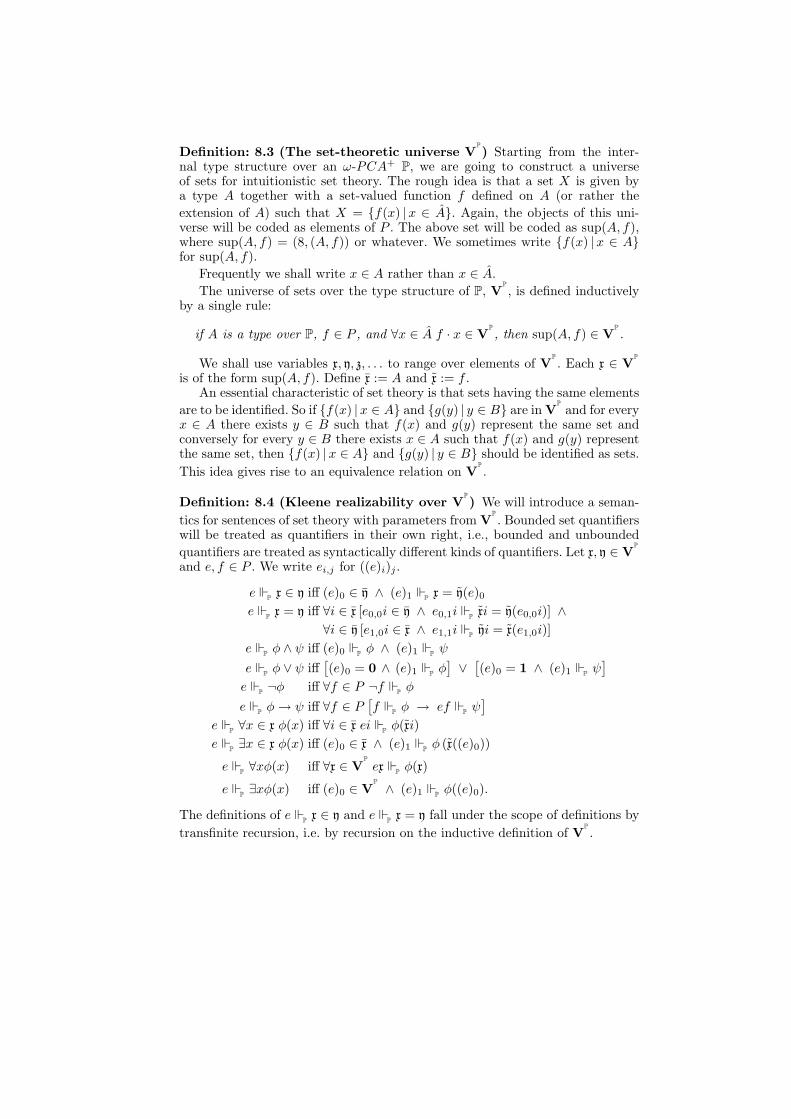
Definition: 8.3 (The set-theoretic universe VP) Starting from the inter-

nal type structure over an ω-PCA+ P, we are going to construct a universeof sets for intuitionistic set theory. The rough idea is that a set X is given bya type A together with a set-valued function f defined on A (or rather theextension of A) such that X = {f(x) |x ∈ A}. Again, the objects of this uni-verse will be coded as elements of P . The above set will be coded as sup(A, f),where sup(A, f) = (8, (A, f)) or whatever. We sometimes write {f(x) |x ∈ A}for sup(A, f).

Frequently we shall write x ∈ A rather than x ∈ A.The universe of sets over the type structure of P, V

P, is defined inductively

by a single rule:

if A is a type over P, f ∈ P , and ∀x ∈ A f · x ∈ VP, then sup(A, f) ∈ V

P.

We shall use variables x, y, z, . . . to range over elements of VP. Each x ∈ V

P

is of the form sup(A, f). Define x := A and x := f .An essential characteristic of set theory is that sets having the same elements

are to be identified. So if {f(x) |x ∈ A} and {g(y) | y ∈ B} are in VP

and for everyx ∈ A there exists y ∈ B such that f(x) and g(y) represent the same set andconversely for every y ∈ B there exists x ∈ A such that f(x) and g(y) representthe same set, then {f(x) |x ∈ A} and {g(y) | y ∈ B} should be identified as sets.This idea gives rise to an equivalence relation on V

P.

Definition: 8.4 (Kleene realizability over VP) We will introduce a seman-

tics for sentences of set theory with parameters from VP. Bounded set quantifiers

will be treated as quantifiers in their own right, i.e., bounded and unboundedquantifiers are treated as syntactically different kinds of quantifiers. Let x, y ∈ V

P

and e, f ∈ P . We write ei,j for ((e)i)j .

e P x ∈ y iff (e)0 ∈ y ∧ (e)1 P x = y(e)0

e P x = y iff ∀i ∈ x [e0,0i ∈ y ∧ e0,1i P xi = y(e0,0i)] ∧∀i ∈ y [e1,0i ∈ x ∧ e1,1i P yi = x(e1,0i)]

e P φ ∧ ψ iff (e)0 P φ ∧ (e)1 P ψ

e P φ ∨ ψ iff[(e)0 = 0 ∧ (e)1 P φ

]∨[(e)0 = 1 ∧ (e)1 P ψ

]e P ¬φ iff ∀f ∈ P ¬f P φ

e P φ→ ψ iff ∀f ∈ P[f P φ → ef P ψ

]e P ∀x ∈ x φ(x) iff ∀i ∈ x ei P φ(xi)e P ∃x ∈ x φ(x) iff (e)0 ∈ x ∧ (e)1 P φ (x((e)0))

e P ∀xφ(x) iff ∀x ∈ VPex P φ(x)

e P ∃xφ(x) iff (e)0 ∈ VP∧ (e)1 P φ((e)0).

The definitions of e P x ∈ y and e P x = y fall under the scope of definitions bytransfinite recursion, i.e. by recursion on the inductive definition of V

P.

Theorem: 8.5 Let P be an ω-PCA+. Let ϕ(v1, . . . , vr) be a formula of set the-ory with at most the free variables exhibited. If

CZF + RDC ` ϕ(v1, . . . , vr)

then there exists a closed application term tϕ of PCA+ such that for all x1, . . . , xr

in VP,

P |= tϕx1 . . . xr ↓

andt

ϕx1 . . . xr P ϕ(x1, . . . , xr).

The term tϕ

can be effectively constructed from the deduction of ϕ(v1, . . . , vr).

Remark: 8.6 A background theory sufficient for carrying out the definition ofV

Pand establishing Theorem 8.5 is KP. More precisely, if KP proves that P

is an ω-PCA+ and CZF + RDC ` ϕ(v1, . . . , vr), then there exists a closedapplication term t

ϕof PCA+ such that KP proves for all x1, . . . , xr ∈ V

P,

P |= tϕx1 . . . xr ↓ and t

ϕx1 . . . xr P ϕ(x1, . . . , xr).

To obtain a similar result for CZF plus the regular extension axiom we need astronger type structure.

Definition: 8.7 Let P = (P, ·, . . .) be an ω-PCA+.The type structure T P

W is defined by adding one more inductive clause toDefinition 8.1.

(7) If A is a type and for each x ∈ A, F (x) is a type, where F ∈ P and F (x)means F · x, then

WP

x:AF (x)is a type with extension S, where S is the set inductively defined by thefollowing clause:

If a ∈ A, f ∈ P , and ∀x ∈ F (a) f · x ∈ S, then p(a, f) ∈ S.

The set-theoretic universe VP

Wis defined in the same vein as V

Pexcept that it

is built over the type structure T PW .

Realizability over VP

Wis defined similarly as in Definition 8.4 with V

P

Wre-

placing VP.

Theorem: 8.8 Let P be an ω-PCA+. Let ϕ(v1, . . . , vr) be a formula of set the-ory with at most the free variables exhibited. If

CZF + REA + RDC ` ϕ(v1, . . . , vr)

then there exists a closed application term tϕ of PCA+ such that for all x1, . . . , xr

in VP

W,

P |= tϕx1 . . . xr ↓

andt

ϕx1 . . . xr P ϕ(x1, . . . , xr).

The term tϕ can be effectively constructed from the deduction of ϕ(v1, . . . , vr).

Remark: 8.9 A background theory sufficient for carrying out the definition ofV

P

Wand establishing Theorem 8.8 is KPi.

9 The set-theoretic universe over Kleene’s second model

Henceforth let U be a subset of NN closed under ‘recursive in’ and the jumpoperator. Let A be Kleene’s second model based on U , i.e. the applicative struc-ture with domain U and application being continuous function application, |.The interpretation of the natural numbers in A that is the interpretation N

Aof

the predicate symbol N in A is the set of all constant functions. We use n todenote the constant function with value n. In particular there are the interpreta-tions kA, sA,0A, sA

N ,pAN ,d

A,pA,pA0 ,p

A1 of the constants of APP in U . We shall,

however, mostly drop the superscript A.Our goal is to show that in addition to the axioms of CZF, V

Aalso realizes

CC and FT. The first step is to single out the elements of VA

that play therole of ω and Baire space ωω. We use variables α, β, γ, . . . to range over U . LetV := V

A. Define

∅ := sup(NA

0 , λα.α)

x′ := sup(x +A N

A

1 , λβ.d(x(p1β), x,p0β,0))

and ∆ ∈ U by

∆ · η ={∅ if η(0) = 0(∆ · (η − 1))′ if η(0) 6= 0,

where η − 1 is the function γ with γ(n) = η(n) − 1 if η(n) > 0 and γ(n) = 0otherwise. The definition of ∆ appeals to the recursion theorem for A.4 Finally,ω is defined by

ω := sup(NA, ∆).

By induction on n one shows that ∆ · n ↓ and ∆ · n ∈ V, thus ω ∈ V.The representation ω of the set of von Neumann integers has an important

property.

Definition: 9.1 We use A A to convey that η A A for some η ∈ U .

x ∈ V is injectively presented if for all α, β ∈ x, whenever

A x(α) = x(β)

then α = β.

Lemma: 9.2 ω is injectively presented.

Proof: We must show that A ∆ · n = ∆ · m implies n = m. This can be verifiedby a routine double induction, first on n and within that on m. For details see[1] Lemma 5.5 or [23] Theorem 4.24. 2

Corollary: 9.3 The Axiom of Countable Choice, ACω, and the Axiom of De-pendent Choices, RDC, are validated in V.4 The recursion theorem for partial continuous function application and other details

of recursion theory in A can be found in [28] 3.7.

Proof: This is an immediate consequence of the injective presentation of ω. Thedetails are similar to the proof of [1] Theorem 5.7 or [23] Theorem 4.26. 2

Next we aim at finding an injective presentation of Baire space in V. We willneed internal versions of unordered and ordered pairs in V.

Definition: 9.4 There is a closed application term OP of APP such that A |=OP ↓ and

A |= OP(α, β, 0) = α ∧ OP(α, β, 1) = β

for all α, β ∈ U . Now let

{x, y}V = sup(NA

2 , λα.OP(x, y, α))

; 〈x, y〉V = {{x, x}V , {x, y}V}Vfor x, y ∈ V. The internal versions of α ∈ U , denoted αV , and of Baire space,denoted BV , are the following:

αV := sup(NA, λγ.〈∆ · γ(0), ∆ · α(γ(0))〉V

)BV := sup(UA, λα.αV).

Corollary: 9.5 For all x, y ∈ V, {x, y}V , 〈x, y〉V ∈ V. For all α ∈ U , αV ∈ V.Moreover, BV ∈ V.

Proof: These claims are obviously true. 2

Corollary: 9.6 BV is injectively presented.

Proof: Let ∆∗(n) := ∆ · n. As a first step, one must show that

A 〈∆∗(n1), ∆∗(m1)〉V = 〈∆∗(n2), ∆∗(m2)〉Vimplies n1 = m1 and n2 = m2. This follows from the fact that

A “〈x, y〉V is the ordered pair of x and y”

holds and that ω is injectively presented according to Corollary 9.2. 2

Notice the important role of the type UA in obtaining an injective presentationof Baire space. This will enable us to verify that CC holds in V.

Lemma: 9.7 There is a closed application term t such that A |= t ↓ and

αt A “BV is the set of all functions from ω to ω”

where t evaluates to αt in A.

Proof: Supposeβ A “f is function from ω to ω”.

Then from β one can distill β∗ such that β∗ A ∀n ∈ ω ∃k ∈ ω 〈n, k〉 ∈ f .

Thus β∗ · n A ∃k ∈ ω 〈∆ · n, k〉 ∈ f , so that (β∗ · n)0 ∈ N A and (β∗ · n)1 A

〈∆ · n,∆ · (β∗ · n)〉 ∈ f . Now define β# by β#(n) = (β∗ · n)0(0). Then one caneffectively construct β�, β[ from β such that β� A f = β#

Vand β[ A f ∈ BV .

Conversely, if γ A f ∈ BV , one can construct γ† from γ such that γ† A“f is a function from ω to ω.”.

As all of the above transformations can be effected by application terms, thedesired assertion follows. 2

Theorem: 9.8 The principles CC and AC2 are valid in V.

Proof: Suppose

η A ∀f ∈ BV ∃n ∈ ω A(f, n). (10)

Then, for all α ∈ U , η · α A ∃n ∈ ω A(αV , n), so that

(η · α)0 ∈ NA ∧ (η · α)1 A A (αV , ∆ · (η · α)0) . (11)

Define

η∗ := sup(UA, λα.〈αV , ∆ · (η · α)0〉V

).

Obviously we can construct a closed term t# such that A |= t# ↓ and with ϑ ∈ Usuch that A |= t# ' ϑ we obtain

ϑ · η A η∗ : BV → ω ∧ ∀f ∈ BV A(f, η∗(f)). (12)

We can thus cook up another closed application term t+ which evaluates to afunction Ξ in A such that

Ξ · η = p(η∗, ϑ · η).

In view of (12) we arrive at

Ξ A ∀f ∈ BV ∃n ∈ ω A(f, n) → ∃F [F : BV → ω ∧ ∀f ∈ BV A(f, F (f))] .

One can also show that the function η∗ in (12) constructed from η is a continuousfunction in the realizability model V. By the previous Lemma 9.7, BV is alsorealizably the Baire space. So the upshot is that CC is realized.

Moreover, for the above proof the restriction of the existential quantifier toω in (10) is immaterial. As a result, the above proof establishes realizabilityof AC2 in V as well, whereby AC2 stands for the following statement: If F isa function with domain NN such that ∀α ∈ NN∃x ∈ F (α) then there exists afunction f with domain NN such that ∀α ∈ NNf(α) ∈ F (α).

Furthermore, a similar proof establishes the realizability of F-CC in V. 2

Theorem: 9.9 Let ϕ(v1, . . . , vr) be a formula of set theory with at most the freevariables exhibited.

(i) IfCZF + CC + FT + AC2 + RDC ` ϕ(v1, . . . , vr)

then there exists a closed application term tϕ of PCA+ such that for allx1, . . . , xr ∈ V

A,

A |= tϕx1 . . . xr ↓

andt

ϕx1 . . . xr A ϕ(x1, . . . , xr).

The term tϕ can be effectively constructed from the deduction of ϕ(v).(ii) Suppose that the domain of A is a β-model and that

CZF + REA + CC + BIM + AC2 + RDC ` ϕ(v1, . . . , vr).

Then there exists a closed application term sϕ

of PCA+ such that for allx1, . . . , xr ∈ V

A

W,

A |= sϕx1 . . . xr ↓and

sϕx1 . . . xr A ϕ(x1, . . . , xr).The term sϕ can be effectively constructed from the deduction of ϕ(v).

Proof: (i): In view of Theorem 8.5 and Theorem 9.8, it suffices to show real-izability of FT. This is basically the same proof as for Theorem 6.5 only in amore involved context. So we omit the details.

(ii): By Theorem 8.8 and Theorem 9.8, it remains to verify realizability ofBIM. This is similar to the proof of Theorem 6.8. 2

Theorem: 9.10 (i) CZF and CZF+CC+FT+AC2 +RDC have the sameproof-theoretic strength and prove the same Π0

2 sentences of arithmetic.(ii) CZF+REA and CZF+REA+CC+BIM +AC2 +RDC have the same

proof-theoretic strength and prove the same Π02 sentences of arithmetic.

(i) follows from Theorem 9.9(i), the fact that the proof of 9.9(i) can be carriedout in the background theory KP, and that CZF and KP prove the same Π0

2sentences.

(ii) follows from Theorem 9.9(ii) together with the insight that the existenceof NN ∩ Lρ (where ρ = supn<ω ωckn ) can be shown in KPi and that KPi is abackground theory sufficient for the construction of V

P

W. Moreover, KPi is of

the same strength as CZF+REA and the theories prove the same Π02 sentences

of arithmetic. 2

The question that remains to be answered is whether BIM adds any strength toCZF. It is shown in [25] that CZFR,E + BID proves the 1-consistency of CZF.

Definition: 9.11 Let CZFR,E be obtained from CZF by replacing Strong Col-lection with Replacement and Subset Collection with Exponentiation, respec-tively.

Note that Strong Collection implies Replacement and that Subset Collectionimplies Exponentiation. Thus CZFR,E is a subtheory of CZF.

Theorem: 9.12 CZFR,E + BID proves the 1-consistency of CZF and KP.

Proof: [25]. 2

References

1. P. Aczel: The type theoretic interpretation of constructive set theory: Choiceprinciples. In: A.S. Troelstra and D. van Dalen, editors, The L.E.J. BrouwerCentenary Symposium (North Holland, Amsterdam 1982) 1–40.

2. P. Aczel: The type theoretic interpretation of constructive set theory: Inductivedefinitions. In: R.B. et al. Marcus, editor, Logic, Methodology and Philosophyof Science VII (North Holland, Amsterdam 1986) 17–49.

3. P. Aczel, M. Rathjen: Notes on constructive set theory, Technical Report40, Institut Mittag-Leffler (The Royal Swedish Academy of Sciences, 2001).http://www.ml.kva.se/preprints/archive2000-2001.php

4. J. Barwise: Admissible Sets and Structures (Springer-Verlag, Berlin, Heidel-berg, New York, 1975).

5. M. Beeson: Foundations of Constructive Mathematics. (Springer-Verlag,Berlin, Heidelberg, New York, Tokyo, 1985).

6. E. Bishop and D. Bridges: Constructive Analysis. (Springer-Verlag, Berlin,Heidelberg, New York, Tokyo, 1985).

7. D. Bridges, F. Richman: Varieties of constructive mathematics. LMS LectureNotes Series 97 (Cambridge University Press,Cambridge,1987).

8. L.E.J. Brouwer: Weten, willen, spreken (Dutch). Euclides 9 (1933) 177-193.9. L. Crosilla and M. Rathjen: Inaccessible set axioms may have little consis-

tency strength Annals of Pure and Applied Logic 115 (2002) 33–70.10. M. Dummett: Elements of intuitionism. Second edition (Clarendon

Press,Oxford,2000)11. S. Feferman: A language and axioms for explicit mathematics. In: J.N. Cross-

ley (ed.): Algebra and Logic, Lecture Notes in Math. 450 (Springer, Berlin1975) 87–139.

12. S. Feferman: Constructive theories of functions and classes in: Boffa, M., vanDalen, D., McAloon, K. (eds.), Logic Colloquium ’78 (North-Holland, Ams-terdam 1979) 159–224.

13. N. Gambino: Types and sets: a study on the jump to full impredicativity, Lau-rea Dissertation, Department of Pure and Applied Mathematics, Universityof Padua (1999).

14. P.G. Hinman: Recursion-theoretic hierarchies (Springer, Berlin, 1978).15. S.C. Kleene, R.E. Vesley: The foundations of intuitionistic mathematics.

(North-Holland,Amsterdam,1965).16. J. Myhill: Constructive set theory. Journal of Symbolic Logic, 40:347–382,

1975.17. M. Rathjen: The strength of some Martin-Lof type theories. Department of

Mathematics, Ohio State University, preprint (1993) 39 pages.18. M. Rathjen: The realm of ordinal analysis. In: S.B. Cooper and J.K. Truss

(eds.): Sets and Proofs. (Cambridge University Press, 1999) 219–279.19. M. Rathjen, R. Lubarsky: On the regular extension axioms and its variants.

Mathematical Logic Quarterly 49, No. 5 (2003) 1-8.20. M. Rathjen Realizability for constructive Zermelo-Fraenkel set theory. To ap-

pear in: J. Vaananen, V. Stoltenberg-Hansen (eds.): Proceedings of the LogicColloquium 2003.

21. M. Rathjen: Choice principles in constructive and classical set theories. Toappear in: Z. Chatzidakis, P. Koepke, W. Pohlers (eds.): Proceedings of theLogic Colloquium 2002.

22. M. Rathjen: Replacement versus collection in constructive Zermelo-Fraenkelset theory. Annals of Pure and Applied Logic, Volume 136, Issues 1-2 (2005)156–174.

23. M. Rathjen: The formulae-as-classes interpretation of constructive set theory.To appear in: Proof Technology and Computation, Proceedings of the Interna-tional Summer School Marktoberdorf 2003 (IOS Press, Amsterdam).

24. M. Rathjen: Realizability interpretations for constructive set theory. To appearin: Logical aspects of secure computer systems, Proceedings of the InternationalSummer School Marktoberdorf 2005 (IOS Press, Amsterdam).

25. M. Rathjen: A note on bar induction in constructive set theory. Math. Log.Quarterly 52 (2006) 253-258.

26. A.S. Troelstra: Metatamathematical investigaton of intuitionistic arithmeticand analysis. Lecture Notes in Mathematics vol. 344 (Springer,Berlin,1973).

27. A.S. Troelstra: A note on non-extensional operations in connection with con-tinuity and recursiveness. Indagationes. Math. 39 (1977) 455–462.

28. A.S. Troelstra and D. van Dalen: Constructivism in Mathematics, Volumes I,II. (North Holland, Amsterdam, 1988).