Constructive recognition of classical groups in their

Journal of Symbolic Computation 35 (2003) 195–239

www.elsevier.com/locate/jsc

Constructive recognition of classical groups intheir natural representation

Peter A. Brooksbank∗

Department of Mathematics, The Ohio State University, 231 W. 18th Avenue, Columbus, OH 43210, USA

Received 4 December 2001; accepted 1 October 2002

Abstract

Let S ⊂ GL(V) be a given set of generators for a groupG, whereV is a finite-dimensionalvector space over a finite fieldF. We present an algorithm which recognises, constructively, whenGis Sp(V),SU(V) or Ωε(V). Our algorithm handles all of those classical groups uniformly and runsin time which is polynomial in the input length, assuming a discrete logarithm oracle forF.c© 2003 Elsevier Science Ltd. All rights reserved.

1. Introduction and results

Let V be a finite-dimensional vector space over the finite fieldF. In this paper wewill use the termclassical form on Vto mean a nondegenerate alternating, Hermitian orquadratic form onV , and aclassical group on Vwill be a perfect subgroup of GL(V)preserving such a form. That is to say, the classical groups onV are just Sp(V),SU(V)or Ωε(V)(ε = +,− or 0): we will refer to these possibilities as casesS,U and O,respectively.

Suppose thatG = 〈S〉 ≤ SL(V) is given. Then one can efficiently test whether or notG preserves a classical form onV and, if it does, one can also obtain a matrix representingsuch aG-invariant form. Hence we may assume thatG is a subgroup of a particularclassical group onV . A nonconstructive recognition algorithm, such as the algorithmof Niemeyer and Praeger (1998), can then be applied to decide whether or notG is thatclassical group. If it is then one can decide via an elementary test whether or not any givenelement of GL(V) is in G. The additional feature of aconstructive recognition algorithmis a routine which, for any given elementg ∈ G, constructs astraight-line program (SLP)from S to g. Constructive recognition algorithms are a key ingredient in the ambitious

∗ Tel.: +1-614-688-3175; fax: +1-614-292-1479.E-mail address:[email protected] (P.A. Brooksbank).

0014-5793/03/$ - see front matterc© 2003 Elsevier Science Ltd. All rights reserved.doi:10.1016/S0747-7171(02)00132-3

196 P.A. Brooksbank / Journal of Symbolic Computation 35 (2003) 195–239

project to construct a composition series for any given matrix group (this has becomeknown as the “computational matrix group project” (Leedham-Green, 2001)).

Because of the size of the groups concerned, all known constructive recognitionalgorithms for finite simple groups employ randomized algorithms rather than the moretraditional deterministic ones. Randomized algorithms for groups fundamentally requirea method of selecting nearly uniformly distributed random elements; such a method isprovided byBabai (1991). A randomized algorithm is calledMonte Carlo if the outputof the algorithm is correct with probability>1/2 (higher reliability can be achievedby repetition and majority vote).Las Vegasalgorithms form a subclass of Monte Carloalgorithms. Here a positive output is guaranteed to be correct, but failure may be reported(with probability<1/2) if a suitable output has not been determined after a prescribedtime. The randomized algorithms presented here will always be Las Vegas.

The principal reason for treating the natural representation separately from otherrepresentations is to make use of algorithmic techniques which are unique to this setting.For example, we will frequently be able simply to write down matrices lying in certainsubgroups and then use linear algebra to construct them from known generators for thatsubgroup. This is a luxury which is not available in other settings and it gives rise to muchfaster algorithms (cf.4.5.1).

Celler and Leedham-Green (1998)provided the first example of this type of algorithmfor the case whenG contains the special linear group SL(V) and Celler (1997)laterdealt with the caseG = Sp(V). In Brooksbank (2001a), a simplified version of ouralgorithm is given which deals only with the caseG = Ω(d,q) for d odd. Our goalhere is a general algorithm for all classical groups with a proven asymptotic runningtime. Hence we both develop more theory and include more detailed proofs than inCeller (1997), Celler and Leedham-Green (1998)andBrooksbank (2001a). We obtain analternative algorithm toCeller (1997)for G = Sp(V) and we will use the timing inCeller (1997)as a measure of the efficiency of our algorithm (cf.1.1and alsoSection 7).

A drawback to the algorithms inCeller (1997)andCeller and Leedham-Green (1998)isthat their running times are not polynomial in the length of the input. In particular, they bothrequire the construction of a multiple ofq random group elements in order to guaranteesuccess with high probability. However, the recent advances of Conder, Leedham-Greenand O’Brien (Conder and Leedham-Green, 2001; Conder et al., 2002) show that explicitoccurrences ofq in the running time of an algorithm for any irreducible representation ofSL(2,q) (over a field having the natural characteristic) can be avoided at the expense ofusing an “oracle” which computes discrete logarithms in GF(q)∗.

In this paper we also assume the availability of a discrete log oracle and use this, togetherwith the algorithm inConder and Leedham-Green (2001), to devise an algorithm whichrecognises constructively any classical group in its natural representation. We will see thatSL(2,q)-subgroups are the heart of the matter; indeed, we will show that SL(2,q) is thepolynomial time bottleneck.

The main advantage of our algorithm is that, while certain subroutines need to beslightly modified for the different classical groups, the architecture of the main algorithmremains the same. That is, we are able to deal with all classical groups simultaneously.The algorithm has been implemented by the author in the computer algebra system

P.A. Brooksbank / Journal of Symbolic Computation 35 (2003) 195–239 197

GAP (The GAP Group, 2000) and the results of some preliminary performance tests aresummarised inSection 7.

Our main result can be stated as follows:

Theorem 1.1. Let G = 〈S〉 ≤ GL(V) be given, where V is a vector space of dimensiond ≥ 2 over the finite fieldGF(q). Then there is a Las Vegas algorithm which, if G is aclassical group on V , finds a new generating setT for G (whose elements are constructedusing SLPs fromS) having the property that an SLP of length O(d2logq) can be foundfromT to any given g∈ G.

Assuming the availability of an oracle to compute discrete logarithms inGF(q)∗, inGF(

√q)∗ if G is unitary, or inGF(q2)∗ in the single case G= Ω−(4,q), the algorithm

for constructingT runs in polynomial time

O(d3logq(d + logdlog3q)+ ξd + log logq + µ|S| + d2log2q + χ logq),

while each application of the deterministic routine to write an SLP fromT takesO(d3logq + log2 q) time.

Hereξ is an upper bound on the time requirement per element for the construction ofindependent, (nearly) uniformly distributed random elements of G,µ is an upper boundon the time required to perform each group operation in G andχ represents the cost, percall, to the appropriate discrete logarithm oracle.

Remarks.

(i) The groups SL(V) could also have been included inTheorem 1.1, but were omit-ted to facilitate a more uniform treatment. An algorithm for SL(V) is given inCeller and Leedham-Green (1998), and suggestions for an improved algorithm, inthe same spirit asTheorem 1.1, are discussed inConder and Leedham-Green (2001).

(ii) The GF(q2)∗ oracle forG = Ω−(4,q) arises from the isomorphismΩ−(4,q) ∼=PSL(2,q2) (cf. 6.1.4).

(iii) As suggested by the statement of the theorem, the basic idea of the algorithm(as inCeller, 1997; Celler and Leedham-Green, 1998) is to construct a setT fromwhich it is easy to write a SLP of modest length to any given elementg ∈ G. InCeller and Leedham-Green (1998), T consists of sufficiently many transvections toperform Gaussian elimination in SL(V). In 5.2 we give a more involved analogueof Gaussian elimination which works inside any classical group, and the setT willconsist of the elements necessary to execute this procedure.

To obtain a comparison of our running time with that of existing algorithms, we statethe following consequence ofTheorem 1.1.

Corollary 1.1. For d ≥ 5, there is an alternative version of the constructive recognitionalgorithm in Theorem1.1 which does not assume a discrete logarithm oracle and con-structsT in time

O(d3logq(d + logdlog4q)+ ξd + log logq + µ|S| + d2log2q + qεlogq),

whereε = 1/2 if G is unitary,ε = 2 if G = Ω−(4,q) andε = 1 otherwise.


Remark. The termqεlogq that appears above arises from the preprocessing required toform a list of the necessary field elements. Discrete logarithms are then found using abinary search in that list.

1.1. Timing comparisons

Perhaps the most important comparison is with the black box classical group algorithmin Kantor (2001)since, if we do not obtain a significantly improved running time over thatalgorithm, one might question the value of treating the natural representation separately.As in Kantor (2001,Theorem 1.1(vii)) (ignoring the cost of verifying a presentation), theblack box algorithm runs in time

O(ξd2qlogdlogq + µ(d4q3/2log2 qlog3d + d5log5/2 q)).

Comparing with the running time inCorollary 1.1it is clear that our algorithm runs muchmore quickly (noting, of course, that our “q2” is their “q” when G = Ω−(4,q) ∼=PSL(2,q2)).

An examination of the subroutines inCeller (1997)for G = Sp(V) reveals that, in ournotation, the main algorithm inCeller (1997)runs in timeO(d2q(ξ + µ)) = O(ξd2q).The coefficient ofξ in Theorem 1.1is d + log logq, so our algorithm uses almost a factorof dq fewer random elements.

2. Classical group preliminaries

We assume a basic familiarity with the classical groups and the geometries associ-ated with them. We will introduce the terminology, notation and theory necessary forour algorithm, but refer the reader toKantor (2001), Kleidman and Liebeck (1990)andTaylor (1992)both for more complete treatments of classical groups and for proofs ofsome elementary results stated here.

Throughout this section, letF = GF(pl ) = GF(q) be a finite field, and letV , anF-space of dimensiond, be the natural module of a classical groupG of Witt index m. Wemay assume thatd > 2 since otherwiseG is solvable or is isomorphic to SL(2,q) (thelatter case is discussed inSection 6.1).

Let k = l/2 in caseU andk = l otherwise. Setq := pk so thatq = q in casesO andS and q = q2 in caseU. In caseO, let ϕ denote a nondegenerateG-invariant quadraticform onV . Let ( , ) denote a nondegenerateG-invariant alternating or Hermitian form incasesS or U respectively, or the symmetric form associated with in caseO. In caseU, let“overbar” denote the involutory automorphismλ → λq of F.

2.1. Standard bases

The moduleV has a standard basisB of one of the following types:

B = e1, . . . ,em, f1, . . . , fm casesS,Ue,O+(d = 2m);B = e1, . . . ,em, v, f1, . . . , fm casesUo,Oo(d = 2m+ 1); orB = e1, . . . ,em, v1, v2, f1, . . . , fm caseO−(d = 2m+ 2).

(1)


Table 1Matrix constraints for casesS,Ue, andO+

CaseS CaseUe CaseO+

ABtr − B Atr = 0 ABtr + BA

tr = 0 ABtr + B Atr = 0

C Dtr − DCtr = 0 CDtr + DC

tr = 0 C Dtr + DCtr = 0

ADtr − BCtr = I ADtr + BC

tr = I ADtr + BCtr = I

Here(ei ,ej ) = ( fi , f j ) = 0, (ei , f j ) = δi j , v, v1, v2 ∈ 〈e1, . . . ,em, f1, . . . , fm〉⊥ and(v, v) = 1 (cf. Kleidman and Liebeck, 1990, Propositions 2.3.2, 2.4.1 and 2.5.3). In caseO−, v1 andv2 behave as in the following lemma.

Lemma 2.1. Let U be a definite line of the orthogonal space V (that is, one which containsno singular vectors) and letρ be a generator ofF∗. Then, replacingϕ with ρϕ if necessary,there exists a basisv1, v2 of U such that

(i) (v1, v2) = 1 andϕ(vi ) = αi for someαi ∈ F∗ (i = 1,2) when q is even; or

(ii) (v1, v2) = 0 and(vi , vi ) = 1 (i = 1,2) when q≡ 3 (mod 4); or

(iii) (v1, v2) = 0, (v1, v1) = 1 and(v2, v2) = ρ, when q≡ 1 (mod 4).

Proof. (i) is trivial. For (ii) and (iii), replacingϕ with ρϕ (and hence ( , ) withρ( , )) ifnecessary, choosev1 such that(v1, v1) = 1 and choosev2 ∈ v⊥1 . Note that the equation(xv1+ v2, xv1+ v2) = x2+ (v2, v2) = 0 has a root inF if q ≡ 1 (mod 4) and(v2, v2) is asquare, or ifq ≡ 3 (mod 4) and(v2, v2) is a nonsquare. The result now follows easily.

We will say that classical groupsG andH areof the same typeif they are both in oneof the casesS,Ue,Uo,O+,Oo,O−; i.e. there are six “types” of classical group. LetFp

denote the prime subfield GF(p) of F and letB be a standard basis ofV . For a generatorρof F

∗, letBρ be the orderedFp-basis obtained fromB by replacing each vectoru ∈ B bythel vectorsu, ρu, . . . , ρl−1u. We callBρ the standardFp-basis obtained fromB andρ.

2.2. Matrices

Let G be a classical group with natural moduleV and letB be a standard basis forV .We now consider the matrix representing an arbitrary element ofG relative toB.

Cases S,Ue,O+ : B = e1, . . . ,em, f1, . . . , fm and elements ofG have the matrix

g =(

A BC D

), (2)

whereA, B,C, D arem×m matrices satisfying the constraints inTable 1. The constraintsarise from the fact thatG preserves ( , ) in each case. There are some additional constraintsin caseO+ whenq is even, arising from the fact thatG also preserves a quadratic form,and we will state these as we need them.


Table 2Matrix constraints for casesUo andOo

CaseUo CaseOo

ABtr + BA

tr + ξ trξ = 0 ABtr + B Atr + ξ trξ = 0

CDtr + DC

tr + ζ trζ = 0 C Dtr + DCtr + ζ trζ = 0

ADtr + BC

tr + ξ trζ = I ADtr + BCtr + ξ trζ = IAωtr + Bηtr + λξ tr = 0 Aωtr + Bηtr + λξ tr = 0Cωtr + Dηtr + λζ tr = 0 Cωtr + Dηtr + λζ tr = 0ηωtr + ωηtr + λλ = 1 ηωtr + ωηtr + λ2 = 1

Cases Uo,Oo: elements ofG have the matrix

g =( A ξ tr Bη λ ω

C ζ tr D

), (3)

whereA, B,C, D arem× m, ξ, η, ω, ζ are 1× m andλ ∈ F satisfying the constraints inTable 2.

Cases O−: elements ofG have the matrix

g =

A ξ tr1 ξ tr

2 Bη1 λ11 λ12 ω1η2 λ21 λ22 ω2C ζ tr

1 ζ tr2 D

. (4)

There are several more constraints of a similar type to those in caseOo above. However,there are three different sets of constraints corresponding to the three different possibilitiesin Lemma 2.1. Furthermore, whenq is even, there are additional constraints arising fromthe fact thatG preserves a quadratic form. We therefore opt to introduce them only as weneed them.

2.3. Transvection groups

A vectorv ∈ V is singular if (v, v) = 0 in casesS andU, or if ϕ(v) = 0 in caseO.Let x be a singular point ofV . In casesS andU,G contains a subgroupT(x) of orderqwhich is the identity onx⊥ and onV/x. The groupT(x) is called thegroupof (x, x⊥)-transvections; G-conjugates ofT(x) are also calledlong root groups of G.

Lemma 2.2 (Kantor, 2001,5.1.2 and 6.1.2).For singular points x= y of V :

(i) if x ∈ y⊥, then〈T(x), T(y)〉 ∼= T(x)× T(y) has order q2; or

(ii) if x /∈ y⊥, then V = 〈x, y〉 ⊥ 〈x, y〉⊥ and 〈T(x), T(y)〉 ∼= SL(2,q) inducing thisgroup on the first summand and the identity on the second.

Remark. We note that Sp(2,q) ∼= SU(2,q) ∼= SL(2,q) (Kleidman and Liebeck, 1990,Proposition 2.9.1(i)).


Table 3The linear transformationsri (w, λ)

Case ri (w, λ) λ |Q|S u → u − (u, w − λei )ei − (u,ei )w λ ∈ F qd−2qU u → u + (u, w − λei )ei − (u,ei )w λ+ λ = (w,w) (q2)d−2qO u → u + (u, w − λei )ei − (u,ei )w λ = ϕ(w) qd−2

2.4. Stabilisers of singular points

Let x and y be the singular points〈e1〉 and〈 f1〉 respectively. The point-stabiliserGx

splits as the semidirect product

Gx = Q(x) Gx,y, (5)

where Q(x) = Op(Gx), the largest normalp-subgroup ofGx. For 1 ≤ i ≤ m andw ∈ 〈ei , fi 〉⊥, let r i (w, λ) be the linear transformation defined inTable 3. Then Q(x)consists of all possible transformationsr1(w, λ).

Let r ′i (w, λ) be the linear transformationr i (w, λ) with all occurrences ofei in Table 3

replaced withfi . ThenQ(y) consists of all possible linear transformationsr ′1(w, λ). The

next result summarises some elementary properties ofQ(x), each of which either is aneasy calculation or is in (Kantor, 2001, 4.1.3, 5.1.3 or 6.1.3).

Theorem 2.1. Let Q = Q(x), let r(w, λ) = r1(w, λ) and let T = T(x) (in casesS andU). Then the following hold:

(i) T is a normal subgroup of Q and consists of all elements r(0, λ) for λ ∈ F, whereλ+ λ = 0 in caseU.

(ii) r (w, λ)g = r (wg, λ) for all g ∈ (Gx,y)′ = Ge1, f1.

(iii) r (w, λ) · r (w′, λ′) = r (w +w′, λ+ λ′ + (w,w′)).(iv) In caseS, [r (w, λ), r (w′, λ′)] = r (0,2(w,w′)); when q is even, Q is elementary

Abelian; when q is odd, Z(Q) = T = Φ(Q) (Frattini subgroup) and Q/T iselementary Abelian.

(v) In caseU, [r (w, λ), r (w′, λ′)] = r (0, (w,w′) − (w′, w)); Z(Q) = Φ(Q) = T andQ/T is elementary Abelian.

(vi) In caseO, Q is elementary Abelian.(vii) Q acts regularly on the set of singular points not perpendicular to x.

Observe that the groupQ (in caseO) or Q/T (in casesS andU) has order|Fd−2|. Infact, it is the natural module of the subgroup(Gx,y)

′ of G.

Corollary 2.1. Let Q = Q in caseO, and letQ = Q/T in casesS andU. Then(Gx,y)′

is a classical group of the same type as G, and the(Gx,y)′-modulesQ and〈x, y〉⊥ are

isomorphic (natural) modules for(Gx,y)′.

Proof. The mapw → r1(w, ϕ(w)) in caseO, andw → r1(w, λ)T (whereλ = 0 in caseS andλ+ λ = −(w,w) in caseU), defines a(Gx,y)

′-module isomorphism〈x, y〉⊥ → Q(this follows fromTheorem 2.1(ii) and (iii)).


Table 4Structure of the subgroupL = GE,F

Case Typical element Constraints |L|S diag(A, A−tr) N

Ue diag(A, A−tr) det(A) = det(A) N/(q + 1)

Uo diag(A, λ, A−tr) λdet(A) = det(A) N

O+ diag(A, A−tr) det(A) = N/(2, q − 1)Oo diag(A,1, A−tr) det(A) = N/2O− diag(A,Λ, A−tr) Eq. (7) (q + 1)N/(2, q + 1)

2.5. Stabilisers of maximal t.s. subspaces

A subspaceU ≤ V is totally singular (t.s.)if (U,U) = 0 in casesS and U, or ifϕ(U) = 0 in caseO. Let E = 〈e1, . . . ,em〉 and F = 〈 f1, . . . , fm〉, both maximal t.s.subspaces ofV . Then the subspace stabilisersGE andGF split as semidirect products:

GE = U(E) L and GF = U(F) L, (6)

whereU(E) = Op(GE),U(F) = Op(GF ) and L = GE,F . We now use the matrixconstraints inTables 1and2 to study the structure of the subgroupsL,U(E) andU(F).

2.5.1. The subgroup LLet q = q2 in caseU andq = q otherwise, and letN = |GL(m, q)|. Forλ ∈ F

∗ writeλ = if λ is a square andλ = otherwise. The structure ofL is summarised inTable 4,whereA ∈ GL(m, q) andΛ ∈ GL(2,q) and the constraints on the matrix entries in caseO− are as follows:

if det(A) =

thenΛ ∈

Ω−(2,q)SO−(2,q)\Ω−(2,q)

. (7)

2.5.2. The subgroups U(E) and U(F)As matrices relative toB we haveU(F) = U(E)tr so we consider only the subgroup

U = U(E). For a row vectorz ∈ Fm, definez to bez in caseU andz otherwise. Define

matricesu(M),u(z,M) andu(z1, z2,M) to be

(I 0M I

),

( I 0 0−z 1 0M ztr I

)and

I 0 0 0zσ(1) 1 0 0zσ(2) 0 1 0M −ztr

1 −αztr2 I

(8)

respectively, whereM ∈ Mm(F), z, z1, z2 ∈ Fm andσ ∈ Sym(2). The structure ofU is

summarised inTable 5where, in caseO−, σ = (1,2) if p = 2 andσ = 1 otherwise, andα = ρ if q ≡ 1 (mod 4) andα = 1 otherwise.

In particular, notice thatU is Abelian only in casesS, Ue and O+. In the othercasesU is a class 2 nilpotent group withZ(U) = u(0,M) in casesUo and Oo andZ(U) = u(0,0,M) in caseO−.


Table 5Structure of the subgroupU

Case Typical element Constraints |U |S u(M) M − Mtr = 0 qm(m+1)/2

Ue u(M) M + Mtr = 0 qm2

Uo u(z,M) M + Mtr + ztrz = 0 qm(m+2)

O+ u(M) M + Mtr = 0a qm(m−1)/2

Oo u(z,M) M + Mtr + ztrz = 0 qm(m+1)/2

O− u(z1, z2,M) M + Mtr + αztr1 zσ(1) + ztr

2zσ(2) = 0a qm(m+3)/2

a Additional constraints exist whenp = 2 since elements ofU also preserveϕ. In caseO+ we haveMii = 0while in caseO− we have(M + ztr

2 z1)ii = (α1ztr1 z1 + α2ztr

2 z2)ii for 1 ≤ i ≤ m, whereα1, α2 are as inLemma 2.1(i).

2.6. Root elements and commutator relations

In casesS and U we have already seen that a long root subgroup ofG is simply atransvection groupT(x) corresponding to a singular pointx. In caseO, a long root groupcorresponds to a t.s. lineΣ in V , its elements inducing the identity on the(d − 2)-spaceΣ⊥. Long root groups in caseO have analogues in casesS andU, where they are calledshort root groups.

Let 0 = w ∈ 〈e1, f1〉⊥ be a singular vector. Along root groupof G in caseO, or ashort root groupin casesS andU, is aG-conjugate of the group

R(e1, w) = r1(λw,0) | λ ∈ F ∼= F+. (9)

The following result, which is easily checked by direct computation, gives some usefulcommutator relations between elements from certain pairs of root groups.

Lemma 2.3. Let G be a classical group and letα, β ∈ F. Then

(i) [r1(αei ,0), r ′1(βej ,0)] = r i (αβej ,0) ∈ U(E) for 1 ≤ i < j ≤ m.(ii) [r1(α fi ,0), r ′

1(β f j ,0)] = r ′i (αβ f j ,0) ∈ U(F) for 1 ≤ i < j ≤ m.

(iii) [r1(αei ,0), r ′1(β f j ,0)] = r i (αβ f j ,0) ∈ L for 1 ≤ i = j ≤ m.

2.7. Primitive prime divisors

By a fundamental theorem ofZsigmondy (1892), if p is a prime andn ≥ 2, then thereis a prime dividingpn − 1 but notpi − 1 for 1≤ i < n, except when eitherp = 2, n = 6,or n = 2 andp is a Mersenne prime. Such a prime is called aprimitive prime divisor(ppd)of pn − 1. We define a ppd#(p; n) to be an integerj > 1 behaving as inTable 6. We callan elementg of a groupG a ppd#(p; n)-elementif |g| is a ppd#(p; n). We also say thatgis a ppd#(p; n1) · ppd#(p; n2)-elementif |g| is both a ppd#(p; n1) and a ppd#(p; n2).

Certain primitive prime divisor elements are highly abundant in classical groups andare useful because of their action on the natural module. The next result gives statisticalinformation about such elements (seeKantor, 2001,4.1.5, 5.1.5 and 6.1.5 for casesO, SandU respectively).


Table 6j is a ppd#(p;n)

n = 1 if p is a Fermat prime then 4| j ;else j is not a power of 2.

if n = 6 andp = 2 then 21| j ;n ≥ 2 else ifn = 2 andp is a Mersenne prime, then 4| j ;

else j is divisible by a ppd ofpn − 1.

Theorem 2.2. Let q= pk ≥ 16, let n ≥ 3 and let G be one ofSp(n,q), SU(n,q) (n odd),or Ω−(n,q). Let V be the natural module of G overF = GF(pl ). Then G contains at least|G|2n (in casesS and O) and |G|

4n (in caseU) elements ofppd#(p; ln)-order and each actsirreducibly on V .

2.8. Probability estimates

We concludeSection 2 by summarising some results that we will need for thecorrectness and reliability proofs of certain subroutines of our main algorithm. The firstresult concerns the natural module of a classical group.

Lemma 2.4. Let V be the natural module of a classical group G of dimension d and letN denote the number of singular points of V .

(i) There areqd−2N/(qδ + 1) hyperbolic lines in V , whereδ is 0 in caseO and is1otherwise.

(ii) With probability>1/4, a randomly selected line in V is hyperbolic.

(iii) If G = Ω+(2m,q) then V has q2m−2(qm − 1)(qm−1 − 1)/2(q + 1) definite lines.

Proof. (i) Fix a singular pointx of V . Each of theqd−1 points not perpendicular toxdetermines a hyperbolic line containingx, each containingq points other thanx. On theother hand, each hyperbolic line containsqδ + 1 singular points.

We prove (ii) only in the case where the lower bound is weakest, namely whenG = Ω−(2m+ 2,q). By (i), sinceN = (qm − 1)(qm−1 + 1) in this case, the proportionof hyperbolic lines is

qd−2(qm − 1)(qm+1 + 1)(q2 − 1)

2(qd − 1)(qd−1 − 1)>

1

2

qd−2(qd+1 − qd−1 − qm+3 + qm+1)

q2d−1 − qd − qd−1 + 1

>1

2

1− q2d−3 + qd+m+1 + qd+m−1 − 2qd

q2d−1 − 2qd

>1

4.

Finally, for (iii), subtract the number of lines of the form〈e,u〉, wheree is singular andu ∈ e⊥ is nonsingular, and the number of hyperbolic and totally singular lines from thetotal number of lines inV . Those which remain are the definite lines.


The following result will enable us to package the most time-consuming computationsof our main algorithm inside a low-dimensional subgroup (cf.4.3.2).

Theorem 2.3. Let G be a classical group with natural module V of dimension d≥ 5with q = pk ≥ 16. Let a∈ G be an element ofppd#(p; k)-order having two-dimensionalnonsingular support[V,a]. Let b be a random G-conjugate of a and let W= [V, 〈a,b〉].

(i) With probability≥1/640, in caseO or if q is even in caseS, 〈a,b〉 inducesΩ+(4,q)on the nonsingular4-space W and1 on W⊥.

(ii) In caseS (q odd), assuming also that a,b areppd#(p; k/2)-elements when k is eventhen, with probability≥1/32, 〈a,b〉 inducesSp(4,q) on the nonsingular4-space Wand1 on W⊥.

(iii) In caseU, assuming also that a,b areppd#(p; k/2)-elements when k is even then,with probability≥1/32, 〈a,b〉 induces SU(4,q) on the nonsingular4-space W and1 on W⊥.

Proof. For (i) seeKantor (2001,Lemmas 4.12(i) and 5.10(i)), for casesO andS respec-tively. For (ii) and (iii), as in Kantor (2001,Lemma 5.10(v)), 〈a,b〉 is an irre-ducible subgroup of the stated group with probability≥1/32. We now refer toKantor and Liebler (1982,Theorems 5.6 and 5.7), for a catalogue of subgroups of Sp(4,q)and SU(4,q) respectively. In each case, there are no proper irreducible subgroups gener-ated by two elements of the stated order having two-dimensional nonsingular support.

Finally, we state additional results that we will use in our treatment of low-dimensionalunitary groups. The first follows fromKantor (2001,Lemma 3.8(ii)), in view of theisomorphism SU(2,q) ∼= SL(2,q).

Lemma 2.5. Let G = SU(2, pk) with pk > 16. Then two elements of the sameppd#(p; 2k)-order generate G with probability>0.55.

Lemma 2.6. Let G= SU(d,q)with d ≥ 4 and q≥ 8, and let T be transvection subgroupof G. With probability>1/2, the group T together with two G-conjugates Tg1, Tg2,generate a subgroup J of G inducing SU(3,q) on the non singular3-space[V, J] and1 on [V, J]⊥.

Proof. As in the proof ofKantor (2001,Lemma 3.7), J acts irreducibly on the nonsingular3-space[V, J] and is the identity on[V, J] with probability at least(1−1/q)4 ≥ (7/8)4 >1/2. The result now follows fromKantor (2001,6.1.4), by noting that there are no proper,irreducible, subgroups of SU(3,q) generated by transvection groups.

3. Algorithmic preliminaries

In this section we outline some elementary procedures which we will use as subroutinesin our main algorithm.

3.1. Matrix groups

We first discuss some issues which arise when computing with matrix groups.


3.1.1. Straight-line programs

It is important, when computing in a group〈S〉, to have an efficient means of recordinghow an elementg ∈ 〈S〉 is constructed fromS (a word inS representingg could haveexponential length).

A SLP of length m fromS to g is a sequence(w1, . . . , wm) such that, for eachi , eitherwi is a symbol representing some element ofS, orwi = ( j ,−1) for j < i (representingthe inverse ofw j ), or wi = ( j , k) for j , k < i (representing the product ofw j andwk),such that if each expressionwi is evaluated sequentially in the obvious way, then the valueof wm is g.

One should think of each symbolwi in such a sequence as being an actual groupelement. However, the rather abstract definition of SLP given above emphasises two things:that we do not store each element of the sequence as a matrix (we evaluate an SLP froma suitable setS only when necessary); and also that SLPs can be written from one set andthen evaluated from another (thus effecting an isomorphism, for example).

3.1.2. Random elements

We will assume that we can generate uniformly distributed random elements of a givenmatrix groupG. A fundamental result ofBabai (1991)gives an algorithm, which runs intime bounded by a polynomial in|S|,d, logq andµ, for computing sufficiently randomelements ofG = 〈S〉 ≤ GL(d,q) (seeKantor, 2001,2.2.2), for a statement and discussionof this result). A more practical, heuristic algorithm is given inCeller et al. (1995).

We introduce a parameterξ in our complexity statements to ensure that the runningtime estimates can easily be adapted to different constructions of random elements inG.However, weassume that ξ ≥ µ|S| since it is presumed that each generator will beinvolved in the construction of a random element.

Reliability claims concerning subroutines which use random elements of a given groupshould take into account the fact that such elements are not taken from a perfectly uniformdistribution. However, our probability estimates will be sufficiently crude so as not to beaffected by small deviations from uniformity. Furthermore, since our algorithm is LasVegas, it will return a correct output no matter what method of random generation is used,including less reliable methods such asCeller et al. (1995).

3.1.3. Element orders and ppds

Computing the exact order of an elementg ∈ G is unnecessary for our purposes, butwe will need to detect properties of|g| so that we can make deductions about the actionof g on the natural module. InTheorem 2.2we saw that certain primitive prime divisorelements occur with high frequency in classical groups. The next result shows that anefficient deterministic test can be applied to any given element ofG to decide whether ornot it has a specified ppd order.

Lemma 3.1. For any prime p and positive integer n, following a one-time integercomputation taking time O(n3log nlog4 p), one can test whether or not any given g∈ Gis a ppd#(p; n)-element in time O(µnlog p).


Proof. In Neumann and Praeger (1992,p. 578), a deterministicO(n3lognlog4 p) algo-rithm is presented which factorspn − 1 = P P′, whereP is the product of all primitiveprime divisors ofpn −1, including multiplicities. For a given integeri , we can computegi

in time O(µlog i ) by repeated squaring. The result now follows by noting thatg ∈ G is appd#(p; n)-element ifgpn−1 = 1 butgP′ = 1. The test is easily modified to accommodatethe more stringent definition given in 2.7.

3.1.4. Normal closures and derived subgroupsWe will need a method for computing derived subgroups inside low-dimensional

classical groups. The following is a special case ofSeress (2002,Theorem 2.4.8).

Proposition 3.1. There is a Monte Carlo O(µ d2log4 dlog2 q + |S|log4 dlogq)-timealgorithm for constructing a generating set of size O(d2logq) for the derived subgroupG′ of G.

Remark. Proposition 3.1will only be applied whend = 3 or 4 in caseU. Hence alloccurrences ofd in the timing will disappear.

We will also employ a deterministic method for finding normal closures in elementaryAbelian sections of a matrix group based on the following elementary fact (which followsfrom Kantor, 2001,Lemma 2.7).

Lemma 3.2. Let Y be aGF(pl )-space, letσ ∈ GL(Y) be appd#(p; nl)-element(n <

dim(Y)), acting irreducibly on the n-space[Y, σ ] and as the identity on a complementarysubspace. For X≤ Y , let Xσ = 〈Xσ i | 0 ≤ i < n〉 ≤ Y . Then the following hold:

(i) Xσ = 〈X〈σ 〉〉.(ii) If X lies in no hyperplane of Y containing[Y, σ ], then Xσ = Y .

3.2. The natural module

We next outline the methods which we will use to compute with the natural moduleV ofour given classical groupG. We assume that we have the matrix representing aG-invariantclassical form relative to a fixed basis ofV (note thatO(d2) field operations are requiredfor each evaluation).

3.2.1. Quadratic equationsSeveral methods are discussed inLidl and Niederreiter (1983)for finding roots of

polynomials over finite fields; we will only need the quadratic case. The timing stated inthe next result arises from theO(l 2) field operations involved in various gcd calculationswhen we specialise to the quadratic case.

Lemma 3.3. There is a Las Vegas O(l 3log p)-time algorithm which, for any given f(x) =x2 + αx + β ∈ F[x] having roots inF, with probability>1− 1/16findsγ1, γ2 ∈ F suchthat f(x) = (x − γ1)(x − γ1).


Remark. The algorithm fails for a reducible inputf (x), with probability<1/16, byincorrectly reporting irreducibility. However, iff (x) happens to be irreducible inF[x],then the algorithm always detects this.

3.2.2. Traces and normsSuppose that we are in caseU so thatl is even,q = pl/2 andλ → λ = λq is an

involutory automorphism ofF with fixed fieldF0 = GF(q).

Lemma 3.4.

(i) There is a deterministic O(l 2logq)-time algorithm which, for any givenβ ∈ F0,findsα ∈ F

∗0 such thatα + α = β.

(ii) There is a Las Vegas O(l 2log2 qlog logq)-time algorithm which, for any givenβ ∈ F

∗0, with probability>1− 1/26 findsα ∈ F

∗ such thatαα = β.

Proof.

(i) This just involves solving a system ofl × l equations overFp.(ii) Use Lemma 3.3at most twice to find a rootγ ∈ F of x2 − β with probability

>1− 1/28. If γ ∈ F0 or γ γ = β then returnα = γ . Otherwise,γ γ = −β and wereturnα = γ δ for δ ∈ F

∗ such thatδδ = −1 found as follows. Ifq ≡ 1 (mod 4)then useLemma 3.3to find a rootδ ∈ F0 of x2 + 1. If q ≡ 3 (mod 4) thenfind the largest integeri such that 2i | q + 1. Usei iterations ofLemma 3.3(atmost 2 log i ! times for each iteration) to find a rootδ ∈ F of x2i + 1. Since(q + 1)/2i is odd, it follows thatδδ = δq+1 = δ2i = −1. The stated timing isfor theO(i logq) = O(logqlog logq) uses ofLemma 3.3. For a fixedi , all 2 log i !applications ofLemma 3.3fail with probability<1/ i 8. Hence, the probability thatat least one iteration fails is<1/ i 7 ≤ 1/27. Hence, the procedure findsα withprobability>1− (1/28 + 1/27) > 1− 1/26.

3.2.3. Standard basesFinally we summarise some algorithmic techniques involved in finding a standard basis

for the natural module of a classical group.

Lemma 3.5. Let U be a nonsingular subspace of V of dimension r. Then in O(rd3logq)-time one can find the orthogonal complement U⊥ to U in V .

Proof. Find the null-space of thed × r matrix [[(vi ,u j )]] over GF(q), wherev1, . . . , vd

is a basis forV andu1, . . . ,ur is a basis forU . The stated timing is that required to obtain[[(vi ,u j )]] using the classical form.

Lemma 3.6. There is a Las Vegas O(d2logq + l 2log2qlog logq)-time algorithm which,for a given2-space L of V does one of the following:

• if L is hyperbolic, returns a hyperbolic pair e, f ∈ V of singular vectors such that(e, f ) = 1 (with probability>1 − 1/16) or incorrectly reports “not hyperbolic”(with probability<1/16);


• if L is not hyperbolic, detects that this is the case.

Proof. Let L = 〈v,w〉 be the given line. First consider caseS. We may assume that(v,w) = 0 since otherwiseL is t.s. (in which case a report of “not hyperbolic” is returned).Outpute := v and f := w/(v,w).

Next consider caseU, and suppose first thatv is singular. Again we may assume that(v,w) = 0 since otherwiseL is not hyperbolic. Sete := v; replacew with w/(v,w); useLemma 3.4(i) to find α ∈ F such thatα + α = −(w,w); and set f := αv + w. If vis not singular, we replace it with a vector that is as follows. Replacew with any vectorin v⊥ ≤ L (wherev⊥ is found usingLemma 3.5). If w is singular, report thatL is nothyperbolic. Otherwise useLemma 3.4(ii) to find α ∈ F such thatαα = −(v, v)/(w,w)and replacev with αv +w.

Finally suppose that we are in caseO. Unlessϕ(v) = (v,w) = 0 orϕ(w) = (v,w) = 0(whenceL is not hyperbolic), useLemma 3.3to find the rootsγ1, γ2 ∈ F of the quadraticϕ(v) + (v,w)x + ϕ(w)x2. If we do not obtain distinctγ1, γ2 ∈ F, report thatL is nothyperbolic. Otherwise sete := v + γ1w and f := (v + γ2w)/(e, v + γ2w).

It is easy to verify in each case that the paire, f behaves as stated. The timing isdominated by the use ofLemma 3.4(ii) and Lemma 3.5, while the stated reliability isthe probability thatLemma 3.4(ii) (caseU) or Lemma 3.3(caseO) succeeds.

Lemma 3.7. There is a Las Vegas O(dlogdd3logq + l 2log2 qlog logq)-time algorithmwhich, with probability>3/4, finds a standard basis of the natural module V .

Proof. The procedure is recursive. IfV = 〈v〉 is a point (hence we are not in caseS),find a scalarα ∈ F

∗ as follows: in caseO, replacingϕ with ρϕ if ϕ(v)(q−1)/2 = 1, useLemma 3.3to find a rootα of x2−ϕ(v)−1; and, in caseU, useLemma 3.4(ii) to find α suchthatαα = −1/(v, v). In each case returnαv (note(αv, αv) = 1 in caseU, andϕ(αv) = 1in caseO).

If L = 〈v,w〉 is a line then useLemma 3.6to find a hyperbolic pair, or else find thatL is probably not hyperbolic. In the former case, we return the pair. In the latter we mayassume that we are in caseO−. Replacingϕ with ρϕ if necessary, useLemmas 3.3and3.5to find and return vectorsv1 andv2 behaving as inLemma 2.1.

Suppose then that dim(V) > 2. Choose up to 6 log (2d)! lines ofV , usingLemma 3.6on each, to find a hyperbolic lineL and hyperbolic paire, f in L. UseLemma 3.5to findthe d − 2 spaceL⊥ (the natural module for a classical group of the same type) and userecursion to find a standard basisB′ for L⊥. Insert the vectorse, f into B′ to obtain astandard basisB for V and returnB.

The stated timing arises from theO(dlogd) uses ofLemma 3.6. A line in V ishyperbolic with probability>1/4 by Lemma 2.4(ii). Hence, if d ≥ 3, the probabilityof failure before the recursive call is<1/(4d2). The entire algorithm therefore fails withprobability≤∑d

3(1/4i 2) < 1/4.


4. The main algorithm

Let G = 〈S〉 be a classical group in its natural representation as a subgroup of SL(V)with V of dimensiond over the fieldF = GF(pl ). In this section, we present an algorithmfor constructing a new generating setT for G using SLPs fromS. In Section 5we willcomplete the proof ofTheorem 1.1by giving a routine for writing an SLP fromT to anygiven elementg ∈ G.

Throughout the entire algorithm, letk, l ,q be as defined at the beginning ofSection 2.Fix a generatorρ of F

∗. Also, in caseU, fix ζ = ρq+1 (a generator ofF∗0) and 0 = δ = −δ

(found usingLemma 3.4(i)). ThroughoutSection 4, we assume thatd ≥ 5 unless statedotherwise.

4.1. Overview of the algorithm

We first give a pseudo-code overview to provide the reader with a reference to thestructure of the algorithm. Appropriate references are listed to the right of the principalsubroutines.

ClassicalConstructiveRecognition(G)Procedure:

M := ClassicalForm (G); [4.2](τ,a) := FindGoodElements (G);(†) [4.3.1]J := ConstructNaturalSubgroup (G,a);(†) [4.3.2]TQ := ConstructQ (J, τ ); [4.4]∆ := ConstructDelta (TQ);(††) [4.5]T := ConstructNewGenerators (∆); [4.6]

ReturnT .

Remarks:

(†) These subroutines are both Las Vegas algorithms; failure may reported at eitherstage. In fact, failure could be reported for two, very different, reasons: eitherG is nota classical group onV ; or it is and bad luck occurred with choices of group elements.We note, however, thatClassicalForm (G) will already have reported failure ifGdoes not preserve an appropriate nondegenerate form onV . Hence failure for the firstreason will only occur whenG is a proper subgroup of the corresponding classicalgroup onV .

(††) Failure will be reported byConstructDeltaexactly when the input setTQ does notgenerate a certain, desired subgroup ofG. This may occur in certain of the cases thatwe consider, but always with low probability.

Small fields:In order to present an algorithm which has a reasonably uniform appearance, itis necessary, at various stages, to avoid pathologies which occur with small fields. However,beyond a particular stage, our algorithm handles all field sizes equally well. Hence, we willassume throughout4.3and4.4thatq ≥ 16; replacements for the routines contained thereinwill be discussed in4.7 for q < 16. Throughout4.5and4.6, we will make no assumptionaboutq.


Table 7The integern

Case n Case n Case n

S d − 2 Uo d − 2 Oo d − 3Ue d − 3 O+ d − 4 O− d − 2

4.2. A G-invariant form

Several methods exist for determining the matrix representing a nondegenerate alternat-ing, symmetric, or Hermitian form left invariant by a given matrix groupG ≤ GL(V) on itsunderlying moduleV . Perhaps the best known of these is the generalisation of the Parker–Norton “meat–axe” algorithm byHolt and Rees (1994). In caseO, one easily obtains aG-invariant quadratic form with given associatedG-invariant symmetric form. Hence, weassume the availability of an efficient algorithm

ClassicalForm(G)[Given: G = 〈S〉 ≤ GL(V).][Find: a (nondegenerate) G-invariant, classical form onV.]

4.3. The subgroup J

Entirely different methods are required whend ≤ 4 and we defer furtherdiscussion of the various low-dimensional groups untilSection 6. The algorithmClassicalConstructiveRecognition for the general case(d ≥ 5) requires that wefirst construct, and then constructively recognise, a suitable low-dimensional subgroupJ.Hence we will soon make calls to certain of the low-dimensional algorithms presented inSection 6.

We will constructJ in two stages. In the first stage, we will search for a frequentlyoccurring elementτ which decomposesV , in a prescribed way, as the sum ofτ -invariantsubspaces. In the second stage we will construct an elementa (usingτ ) such that[V,a] isa hyperbolic line. With high probability,J is generated bya together with a single randomconjugate ofa. Recall thatq ≥ 16 for the remainder of4.3.

4.3.1. The elementsτ and aLet n be the integer defined inTable 7: and letz = nl/2k (sincen is odd only in caseU,

wherel = 2k, z is an integer). We now describe a subroutine which constructs, with highprobability, elementsτ,a ∈ G with the following properties:τ has ppd#(p; nl)-order (orppd#(p; 2k) · ppd#(p; nk)-order in caseO+), such thatτq2−1 centralises a hyperbolic lineof V ; anda := τ (q+1)(qz+1) has ppd#(p; k)-order (or ppd#(p; k) · ppd#(p; k/2)-order ifkis even in casesU andS) whose support is a hyperbolic line centralised byτq2−1.

The procedure is given primarily for caseO+, with the necessary modifications for theother cases given in parentheses. Also, we will prove correctness only in caseO+; the othercases are similar, but easier.


FindGoodElements (G)Procedure:For up to 96n choicesτ ∈ Gif (|τ | = ppd#(p; nk) and |τ | = ppd#(p; 2k)) then

[omit the|τ | = ppd#(p; 2k) test for all other cases]

a := τ (q+1)(qn/2+1);if (|a| = ppd#(p; k) anddim[V,a] = 2) then

[test also|a| = ppd#(p; k/2) if k is even in casesS andU ]Return(τ,a).

Correctness:Since(qn/2 + 1,q − 1) = (q + 1,q − 1) ≤ 2, if a pair (τ,a) is returnedby the procedure, thenτ has ppd#(p; k) · ppd#(p; 2k) · ppd#(p; nk)-order. Furthermore,by Niemeyer and Praeger (1998,Lemma 5.1), any element of order|τ | splits V as aperpendicular direct sumV = V−

4 ⊥ V−d−4, whereVε

i denotes a nonsingulari -spaceof type Oε. In addition, sincea has two-dimensional support,τ preservesV = V+

2 ⊥V−

2 ⊥ V−d−4, wherea centralises thed − 2-spaceV−

2 ⊥ V−d−4 andτq2−1 centralisesV2.

Hence, any pair(τ,a) returned by the procedure behaves as stated.Conversely, any elementτ having ppd#(p; k) · ppd#(p; 2k) · ppd#(p; nk)-order which

preserves a decompositionV = V+2 ⊥ V−

2 ⊥ V−d−4 will be returned by the algorithm

provided that it is divisible also by 16 wheneverp is Mersenne andk = 2, and wheneverp is Fermat andk = 1 (cf. Table 6). We claim that there are at least|G|/32n suchelements ofG. In fact, since our estimates are crude, we need not concern ourselveswith the additional divisibility requirement on|τ | in the Mersenne and Fermat cases.Assuming that our claim is true, the procedure will fail to find a pair(τ,a) with probability≤(1− 1/32n)32n3 < 1/e3.

We first count the number of such elements preserving a fixed decompositionV =V+

2 ⊥ V−2 ⊥ V−

d−4. Recall thatO±(2,q) is dihedral of order 2(q ∓ 1). There are at least

(q + 1)/2 elements ofD2(q+1) of ppd#(p; 2k)-order and at least(q − 1)/2 elements ofD2(q−1) of ppd#(p; k)-order. Hence, byTheorem 2.2, there are at least

q + 1

2

q − 1

2

|Ω−(d − 4,q)|2(d − 4)

= (q2 − 1)|Ω−(d − 4,q)|8(d − 4)

(10)

suitable elements preserving our fixed decomposition. Next, byLemma 2.4(i) and (iii),there are exactly

q2m−4(qm−1 − 1)(qm−2 − 1)

2(q + 1)

qd−2(qm − 1)(qm−1 + 1)

2(q − 1)

(11)

such decompositions ofV (whered = 2m). Hence, multiplying together(10)and(11), wesee that there are at least|Ω+(d,q)|/32(d − 4) = |G|/32n suitable elements inG, asclaimed.

Timing:ConstructingO(d) random elements ofG and usingLemma 3.1up to three timeson each to test the appropriate ppd property costsO(d3logdlog4 q + dξ + µdlogq).Reliability: 1− 1/e3.


Table 8The subgroupJ

Case S (q even) andO S (q odd) U

J ∼= Ω+(4,q) Sp(4,q) SU(4,q)

4.3.2. Constructing JIn 4.3.1we constructed an elementa of ppd#(p; k)- or ppd#(p; k/2) · ppd#(p; k)-order.

We now present an algorithm to construct a naturally embedded four-dimensional subgroupJ of G behaving as inTable 8.

ConstructNaturalSubgroup (G,a)Procedure:For up 3· 210 conjugatesb = ag

J := 〈a,b〉; VJ := [V, J]; [ J is1 on V⊥J ]

if (VJ is a nonsingular 4-space)thenK := the 4× 4 matrix group induced byJ on VJ ; [K ∼= J]TK := ClassicalConstructiveRecognition (K )(∗)if (K is the group defined inTable 8) then

ReturnJ, K ,TK .

(∗) Using the appropriate low-dimensional routine fromSection 6.

Correctness:Since J is 1 on [V, J]⊥, it follows that K embeds naturally inG as thesubgroupJ.

Reliability: Sincea is a ppd#(p; k)- or ppd#(p; k/2) · ppd#(p; k)-element having two-dimensional support, it follows fromTheorem 2.3that, with probability≥1/640, Jinduces the desired subgroup on the nonsingular 4-spaceVJ . For such a subgroupJ,ClassicalConstructiveRecognition (K ) succeeds with probability at least 3/4, soa single conjugateb produces a constructively recognisedK with probability at least(3/4)(1/640) > 1/210. Hence, at least one of our choices succeeds with probability≥1− [(1− 1/210)210]3 > 1− 1/e3.

Timing: O(ξ log logq + log2 q + χ), dominated by the cost of recognisingK in caseU(cf. 6.4.8).

4.3.3. A standard basis for VThe 4-spaceVJ is the natural module forJ. Observe that whenq is even in caseS, VJ

is the natural module for both Sp(4,q) andΩ+(4,q). Although J is the latter group, weview VJ as a subspace of the symplectic moduleV (i.e. we ignore the quadratic form onVJ constructed in4.3.2).

The elementa preserves the decompositionV = [V,a] ⊥ [V,a]⊥ and fixes exactlytwo singular pointsx = 〈e〉 and y = 〈 f 〉 of the hyperbolic line[V,a]. The followingprocedure finds a standard basisB for V , containing vectors spanningx andy, such thatB ∩ VJ is a standard basis forVJ .


Procedure: e1 := e; f1 := f/(e, f ); [e1, f1 is a hyperbolic pair]UseLemma 3.5to find VJ ∩ [V,a]⊥ and then useLemma 3.6to find ahyperbolic paire2, f2 in this line;e1,e2, f1, f2 is a standard basis forVJ .UseLemma 3.5again to findV⊥

J ≤ V and useLemma 3.7to find a standardbasisB′ of V⊥

J .Inserte1,e2, f1, f2 in the appropriate positions ofB′ to obtain a standardbasisB of V and returnB.

Timing and reliability: Lemma 3.7succeeds with probability>3/4 in time O(dlogdd3logq + l 2log2 qlog logq).

4.3.4. Changing basis

For the remainder of the algorithm, we will write matrices ofG relative to the basisBof V constructed in4.3.3. We now have a convenient embedding ofK into J (the groupsreturned byConstructNaturalSubgroup) sending

(A BC D

)→

A 0 B 00 Id−m−2 0 0C 0 D 00 0 0 Im−2

, (12)

whereA, B,C, D are 2× 2 matrices satisfying the set of constraints for caseS, Ue or O+in Table 1, andI j is the j × j identity matrix for j = m− 2, d − m− 2.

LetTJ denote the image ofTK under this embedding.

Timing: O(µ(|S| + logq)) to apply the change of basis matrix to each generator ofG andto each of our constructed elements.

4.4. The subgroups Q(x) and Q(y)

The ability to construct and manipulate the subgroupsQ(x) and Q(y) (described in2.4) is the key to our construction of the new generating setT for G. Henceforth, it willbe understood that (analogues of) all subroutines pertaining toQ(x) are repeated forQ(y)and we make no further mention of the latter. DenotingQ(x) simply byQ, our first goal isto construct a generating setTQ for Q.

In casesS and U, let T denote the transvection groupT(x) and let t1, . . . , tk begenerators forT defined as follows:

t j :=

r1(0, ρ j−1) in caseSr1(0, ζ j−1δ) in caseU

for 1 ≤ j ≤ k. (13)

4.4.1. Constructing Q∩ J

The following procedure returns a generating set for the subgroupX = Q ∩ J.


ConstructSubgroupOfQ (J)Procedure:InitialiseTX := ∅.for i ∈ 1, . . . , l do

WriteSLP (r1(ρi e2,0), J).

WriteSLP (r1(ρi f2,0), J). [Section 6]

TX := TX ∪ r1(ρi e2,0), r1(ρ

i f2,0).if (X is non-Abelian)then

for j ∈ 1, . . . , kWriteSLP(t j ,TJ). [Section 6]TX := TX ∪ t j .

ReturnTX.

Correctness: Qconsists of all elements ofG which induce 1 onx and onx⊥/x. SinceJcentralises the(d − 4)-spaceV⊥

J , it follows thatOp(Jx) ≤ Q. HenceQ ∩ J is generatedby TX.

Timing: O(logq(χ + logq)) to write the≤5k SLPs.

Remark:Whenq is even in caseS, X = Op(Ω+(VJ)x) of orderq2, a proper subgroup ofthe more desirable groupOp(Sp(VJ)x) of orderq3; we have not yet explicitly constructedthe transvection groupT at this stage. We will soon be able to constructT even in thiscase, albeit indirectly.

4.4.2. Constructing QWe now give the main procedureConstructQ which returns a generating setTQ for a

subgroup ofQ. In casesS (q odd),Uo andO−, we will always have〈TQ〉 = Q. In theother cases it could happen (with probability<1/8) that〈TQ〉 is a proper subgroup ofQ.There is, however, no randomised component to the following procedure; the success, orotherwise, in generatingQ is determined by previous constructions and will be establishedlater in4.5.

ConstructQ (J, τ )Procedure:

σ := τq2−1;TX := ConstructSubgroupOfQ(J);

Return

TQ :=d−2⋃i=0

(TX)σ i. (14)

Correctness:Recall that〈e1, f1〉 = [V,a] soσ = τq2−1 centralises the 1-spacex = 〈e1〉.Hence,σ normalisesQ(x) by Theorem 2.1(ii), so U = 〈TQ〉 ≤ Q as claimed. Note alsothatU is the normal closure〈X〈σ 〉〉; this follows fromLemma 3.2(ii).

Reliability: For any subgroupY of Q, denote byY the quotient groupY/T if Q isnon-Abelian orY if Q is Abelian. SinceT is the Frattini subgroup ofQ in the non-Abeliancases, it suffices to show thatU = Q with high probability.

Recall the integern defined inTable 7. In each of the six cases,σ acts on the moduleQ, is irreducible on the nonsingularn-space[Q, σ ], and is the identity on the orthogonal


complement[Q, σ ]⊥ of [Q, σ ] in Q. By Lemma 3.2(ii), it suffices to show that, with highprobability, the hyperbolic lineX is in no hyperplane ofQ containing[Q, σ ]. Observe thatX was determined by the random conjugateb = ag (cf. 4.3.2) and is independent of then-space[Q, σ ].

CasesS (q odd),Uo andO−: Heren = d − 2, σ is irreducible onQ, so there are nosuch hyperplanes ofQ. The procedure is deterministic for these cases.

CasesUe and Oo: Here we compute the probability that the lineX lies insidethe nonsingular hyperplane[Q, σ ]. In caseU the probability is(q2)d−5(qd−4 − 1)×(qd−3 + 1)/(q2)d−4(qd−2 − 1) (qd−3 + 1) < 1/q4. In caseOo, the probability isqd−5(q(d−5)/2 − 1)(q(d−3)/2 + 1)/qd−4 (q(d−3)/2 − 1)(q(d−3)/2) + 1) < 1/q2.

CaseS (q even): HereX is a line in thed−1-dimensionalorthogonal spaceQ. Hence theprobability thatX lies in the hyperplane[Q, σ ] is qd−4(q(d−4)/2−1)(q(d−2)/2+1)/qd−3

×(q(d−2)/2 − 1)(q(d−2)/2 + 1) < 1/q2.CaseO+: Heren = d − 4 and there areq + 1 hyperplanes containing then-space

[Q, σ ]. By a counting argument similar to the one above, the probability thatX is in oneof theseq + 1 hyperplanes is<(q + 1)/q2 < 2/q < 1/8.

Hence, in all cases,U = Q with probability>7/8.

Timing: O(µlogdlog2 q) to constructTQ using SLPs fromTX ∪ σ .4.5. The generating sets∆(x) and∆(y)

This is the point at which our differing methods forq ≥ 16 andq < 16 converge; theremaining subroutines handle all field sizes uniformly. At the current stage of the algorithmwe have constructed the following (cf.4.7whenq < 16):

• a standard basisB of V relative to which all matrices are written;• probable generating sets for the subgroupsQ = Q(x) andQ(y); and• generating sets forT(x) < Q(x) andT(y) wheneverQ(x) is non-Abelian.

We will now define the elements of standard generating sets∆(x) for Q(x) and∆(y)for Q(y). As in 4.4, we will only discuss the groupQ = Q(x) and therefore denote∆(x) simply by ∆. We will give a procedureConstructDelta which constructs∆using SLPs from the setTQ returned byConstructQ. The procedureConstructDeltais deterministic in the sense that it will return the desired set∆ if 〈TQ〉 = Q, and failotherwise. This important property ofConstructDeltanotwithstanding, the real purposeof the sets∆(x) and∆(y) is to enable us to construct the generating setT of Theorem 1.1.

4.5.1. Linear algebra inQFor computational purposes, we wish to regard the groupQ as anFp-space relative to

a suitable basis (denoted∆). More precisely, we wish to write

Q =∏v∈∆

〈v〉

such that the decomposition of any givenu ∈ Q, as anFp-vector relative to∆, can beefficiently found. We may then store generators forQ asFp-vectors and also compute in

Q as efficiently as in the row spaceFl(d−2)p .


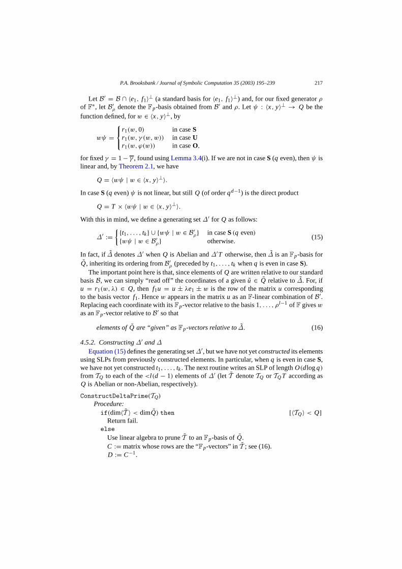
Let B′ = B ∩ 〈e1, f1〉⊥ (a standard basis for〈e1, f1〉⊥) and, for our fixed generatorρof F

∗, let B′ρ denote theFp-basis obtained fromB′ andρ. Let ψ : 〈x, y〉⊥ → Q be the

function defined, forw ∈ 〈x, y〉⊥, by

wψ =

r1(w,0) in caseSr1(w, γ (w,w)) in caseUr1(w, ϕ(w)) in caseO,

for fixedγ = 1− γ , found usingLemma 3.4(i). If we are not in caseS (q even), thenψ islinear and, byTheorem 2.1, we have

Q = 〈wψ | w ∈ 〈x, y〉⊥〉.In caseS (q even)ψ is not linear, but stillQ (of orderqd−1) is the direct product

Q = T × 〈wψ | w ∈ 〈x, y〉⊥〉.With this in mind, we define a generating set∆′ for Q as follows:

∆′ :=t1, . . . , tk ∪ wψ | w ∈ B′

ρ in caseS (q even)wψ | w ∈ B′

ρ otherwise.(15)

In fact, if ∆ denotes∆′ whenQ is Abelian and∆′T otherwise, then∆ is anFp-basis forQ, inheriting its ordering fromB′

ρ (preceded byt1, . . . , tk whenq is even in caseS).The important point here is that, since elements ofQ are written relative to our standard

basisB, we can simply “read off” the coordinates of a givenu ∈ Q relative to∆. For, ifu = r1(w, λ) ∈ Q, then f1u = u ± λe1 ± w is the row of the matrixu correspondingto the basis vectorf1. Hencew appears in the matrixu as anF-linear combination ofB′.Replacing each coordinate with itsFp-vector relative to the basis 1, . . . , ρl−1 of F giveswas anFp-vector relative toB′ so that

elements ofQ are “given” as Fp-vectors relative to∆. (16)

4.5.2. Constructing∆′ and∆Equation (15)defines the generating set∆′, but we have not yetconstructedits elements

using SLPs from previously constructed elements. In particular, whenq is even in caseS,we have not yet constructedt1, . . . , tk. The next routine writes an SLP of lengthO(dlogq)from TQ to each of the<l (d − 1) elements of∆′ (let T denoteTQ or TQT according asQ is Abelian or non-Abelian, respectively).

ConstructDeltaPrime(TQ)

Procedure:if(dim〈T 〉 < dimQ) then [〈TQ〉 < Q]

Return fail.else

Use linear algebra to pruneT to anFp-basis ofQ.C := matrix whose rows are the “Fp-vectors” inT ; see (16).D := C−1.


for i in 1, . . . , l (d − 2)UseD[i ] to write an SLP fromT to thei th element of∆.

if (Q is Abelian)then [∆′ = ∆]Return list of SLPs to∆.

else [∆′T = ∆]Modify the SLPs to∆ to ones fromTQ to ∆′ usingt1, . . . , tk.Return the list of SLPs to∆′.

Correctness: Cis a base change matrix from∆ to the elements ofT , soD is a base changematrix from T to ∆ (the i th row D[i ] gives thei th element of∆ as anFp-vector relativeto T ).

Timing: O(d2log2 q) to write O(kd) SLPs of lengthO(dlogq). Observe that we do notevaluate those SLPs; they just serve to record how the elements of∆′ were constructedfrom TQ.

Remarks:

1. The procedureConstructDeltaPrime is the first time that we used methodswhich depend heavily upon having the natural representation to hand. We wereable simply to write down the matrices inQ that we wanted and then constructthem fromTQ using linear algebra. This process is both much harder and muchless efficient inside a black box elementary Abelian group (see, for example,Kantor, 2001,3.4, 4.4, 5.4, 6.4).

2. Whenq is even in caseS, we have now constructed the elementsti = r1(0, ρ i )

generatingT using SLPs fromTQ. This brings to an end the annoying subdivisionof caseS.

3. If ConstructDeltaPrime is successfully executed then we know that the inputgroup G contains the appropriate classical group (if, for some reason, this is stillin doubt). For, each classical group is generated by the groupsQ(x) andQ(y) whichhave now been shown to be subgroups ofG.

Finally, we define and construct our desired generating set∆. The timing of thefollowing procedure is dominated by that ofConstructDeltaPrime.

ConstructDelta (TQ,TX)

Procedure:∆′ := ConstructDeltaPrime (TQ).if (Q is Abelian)then [∆ = ∆′]

Return∆′.else

Return∆ := t1, . . . , tk ∪ ∆′. [t1, . . . , tk ⊂ TX]4.6. The generating setT

We have now constructed, using SLPs from the original generators, the precise sets∆(x) and∆(y) that we need to construct our target generating setT for G. We first redefine∆ to be the union of those sets:

∆ := ∆(x) ∪ ∆(y). (17)


Although ∆ generatesG, we need the larger setT in order to execute the SLP routinegiven inSection 5.

Recall the subgroupsL,U(E) andU(F) defined in Theorem 6; generators for these keysubgroups will comprise the lion’s share of our generating setT . We first give a pseudo-code overview of the main procedure which constructsT from ∆.

ConstructNewGenerators (∆)Procedure:TL := ConstructL (∆); [4.6.1]TE := ConstructUpperU (∆,TL); [4.6.2]TF := ConstructLowerU (∆,TL); [4.6.2](K ,VK ) := the subgroup and support defined inTable 9; [4.6.3]if (K = J) or (q < 16) thenSK := K ∩ ∆; [identify SK with 4× 4 matrices induced on VK ]TK := ClassicalConstructiveRecognition (〈SK 〉)(†);

[Section 6, or Section 4in caseO−]elseTK := TJ;

TU := ConstructUsefulElements (TE); [4.6.4]ReturnT := TL ∪ TE ∪ TF ∪ TK ∪ TU .

(†) The routineClassicalConstructiveRecognition applied to the low-dimen-sional subgroupK succeeds with probability>1/2. We repeat the procedure, inthe present setting, up to six times to ensure that we successfully obtainTK withprobability>1− 1/64.

4.6.1. The setTL

Here and in4.6.2 we will construct elements ofG using commutators of elementsfrom ∆. It is clear that a short SLP can easily be written fromg,h to [g,h]. For1 ≤ i , j ≤ m and 0 ≤ a < l , we haver1(ρ

a f j ,0) ∈ ∆(x) and r ′1(ei ,0) ∈ ∆(y).

The following procedure produces theO(kd2) elements of the set

TL := r i (ρa f j ,0) | 1 ≤ i = j ≤ m,0 ≤ a < l . (18)

ConstructL (∆)Procedure: InitialiseTL := ∅;for i ∈ 2, . . . ,mfor i = j ∈ 2, . . . ,mfor a ∈ 0, . . . , l − 1

TL := TL ∪ [r1(ρaei ,0), r ′

1( f j ,0)];ReturnTL .

Correctness:By Lemma 2.3(iii), r i (ρa f j ,0) = [r1(ρ

aei ,0), r ′1( f j ,0)].

Timing: O(kd2) (again, we do not evaluate the commutators since we already know towhich group elements they evaluate).

Proposition 4.1 (Gaussian elimination).The group〈TL〉 inducesSL(E) (respectivelySL(F)) on the t.s. subspace E (respectively F) of V . If the linear transformation induced


by g ∈ 〈TL 〉 on E is represented by the matrix M relative to the basis e1, . . . ,em, thenthe linear transformation induced on F has matrixM−tr relative to f1, . . . , fm, where

M = M in caseU and M = M otherwise. Furthermore, if g=(

A ∗∗ ∗

)where A is

m× m, then there are procedures to solve the following problems in O(d3logq) time:

(N) If A is nonsingular, find g′ ∈ G, having “A” entry diag(α,1, . . . ,1) for someα ∈ F

∗, and also find SLPs of length O(d2logq) fromTL to elements g1, g2 ∈ 〈TL 〉such that g1gg2 = g′.

(S) If rank(A) = r < m, find a matrix g′ ∈ G, having “A” entry

(Ar 00 0

), where

Ar is an r × r matrix diag(α1, . . . , αr ) for αi ∈ F∗, and also find SLPs of length

O(d2logq) fromTL to elements g1, g2 ∈ 〈TL〉 such that g1gg2 = g′.

Remark:In the nonsingular and singular cases (N) and (S) above, we arenot saying thatwe actually find the matricesgi (this would requireO(d5log2 q)-time to evaluate the SLPsfrom TL to eachgi ); we need only SLPs to thegi .

Proof. For 1≤ i , j ≤ m andλ ∈ F, let Ei j (λ) denote the elementarym× m matrix withλ in position(i , j ) and zeros elsewhere, and letXi j (λ) be the transvectionIm + Ei j (λ). Asimple calculation shows that the linear transformation induced onF by r i (ρ

a f j ,0) ∈ TL

has matrixXi j (ρa). Hence〈TL 〉 induces SL(F) on F as claimed. That the action of

g ∈ 〈TL〉 on E and F is as stated follows fromTable 4. Finally, the procedures (N) and(S) both use Gaussian elimination in SL(E) with the transvections induced onE by theelements ofTL . In particular, the timing and length of SLPs is as stated.

4.6.2. The setsTE andTF

There are both “lower” and “upper” versions of the proceduresConstructU forconstructing generators forU(E) and U(F) respectively. We only give procedures forU = U(E). We begin with a subroutine for constructing a useful element of〈TL〉.ConjugatingElement (TL)

Procedure:Write down the matrix of any elementc of 〈TL〉 ≤ L such thatc : e1 → e2 → · · · → em. UseProposition 4.1to write an SLP of lengthO(d2logq) from TL to c and returnc together with this SLP.

The structure ofU varies depending on the type ofG (cf. 2.5.2). The next subroutineconstructs generators for the centre ofU (recall that∆(x) contains the transvectiontb ∈ Tfor 1 ≤ b ≤ k).

ConstructCentreOfU (∆, c)Procedure:InitialiseT (1)

E := ∆ ∩ Z(U).for i ∈ 1, . . . ,m− 1for b ∈ 1, . . . , k [only in casesU andS]

T (1)E := T (1)

E ∪ (tb)ci ;for i < j ∈ 1, . . . ,m


for a ∈ 0, . . . , l − 1T (1)

E := T (1)E ∪ [r1(ρ

aej ,0), r ′1(ei ,0)];

ReturnT (1)E

Correctness:By Lemma 2.3(i), r i (ρaej ,0) = [r1(ρ

aej ,0), r ′1(ei ,0)]. In casesU and

S, T(〈ei+1〉) = T(〈e1〉)ci = 〈(tb)ci | 0 ≤ b < k〉 for 1 ≤ i ≤ m− 1. Note thatr i (ρaej ,0)

has matrix

u(Ei j (ρa)− Ej i (ρ

a)), u(0, Ei j (ρa)− Ej i (ρ

a)) or u(0,0, Ei j (ρa)− Ej i (ρ

a)),

while elements ofT(〈ei 〉) have matrixu(Eii (λ)) or u(0, Eii (λ)). It follows thatT (1)E is a

basis for theFp-spaceZ(U), as required.

Timing: O(kd2), as in4.6.1We now give the main procedure for constructing nice generators forU from ∆ ∪ TL

(recall that∆ containsua = r1(ρav, λa) in casesOo andU, andua,s = r1(ρ

avs, λa,s) fors = 1,2 in caseO−, whereλa = ϕ(ρav) in caseOo, λa + λa = −(ρρ)a in caseU, andλa,s = ϕ(ρavs) in caseO−).

ConstructU (∆,TL)

Procedure:c := ConjugatingElement (TL);T (1)

E := ConstructCentreOfU (∆, c);InitialiseT (2)

E := ∅. [generators for U/Z(U)]if (U is non-Abelian)then

for i ∈ 1, . . . ,m− 1for a ∈ 0, . . . , l − 1

Add (ua,1)ci, (ua,2)

ci in caseO−, or else(ua)ci

, toT (2)E .

ReturnTE := T (1)E ∪ T (2)

E .Correctness:Assume thatU is non-Abelian (and hence a class-2 nilpotent group), andconsider just the caseO−. Forλ ∈ F and 1≤ i < j ≤ m, let

εi (λ) = the row vector inFm with λ in coordinatei and zeros elsewhere. (19)

ThenT (2)E is the set of allr i (ρ

avs, λa,s), where 1≤ i ≤ m, 0 ≤ a < k ands = 1,2,having matrixu(εi (ρ

a),0,M1) or u(0, εi (ρa),M2) for s = 1, or 2 respectively. It follows

thatT (2)E projects onto anFp-basis of thek(d − 2)-spaceU/Z(U).

Timing: O(d3logq), dominated by time required to constructc.

4.6.3. The subgroup KOur new generating setT , output by subroutineConstructNewGeneratorsdescribed

on p. 26, contains generators for a certain naturally embedded subgroupK . That subgroup,along with its supportVK , is defined inTable 9(recall thatJ andVJ were constructed in4.3). In the SLP algorithm inSection 5, our strategy will be to modify a given matrixg sothat it lies insideK .


Table 9The subgroupK

Case VK K

S (q odd) VJ J = Sp(VJ )

S (q even) VJ Sp(VJ) > JUe VJ J = SU(VJ)

Uo 〈e1, v, f1〉 SU(VK )

O+ VJ J = Ω+(VJ)

Oo VJ J = Ω+(VJ)

O− 〈e1,e2, v1, v2, f1〉 Ω(VK )

Table 10The elementsxr

Case S,U Oo,O− O+

xr = ∏mi=r+1 ri (0, α)

∏mi=r+1 ri (v∗, ϕ(v∗))

∏t−1i=0 rm−i (em−r+1−i,0 )

Remark:In caseO−, K is a five-dimensional group rather than the more natural choiceΩ−(4,q). This is to avoid squaring the size of the field to recognise the latter group (cf.6.1.4).

Timing: O(ξ log logq + µlog2 q + χ), the timing stated inTheorem 1.1for d = 5 incaseO−.

4.6.4. Some useful elementsFinally, we construct in timeO(µd) a setTU of m (or possibly(m/2)) elements to be

used in the subroutineUpperReduce of WriteSLP (cf. 5.2.1). In Table 10, the scalarα is 1(respectively 0= δ = −δq) in caseS (respectivelyU), and the vectorv∗ is v (respectivelyv1) in caseOo (respectivelyO−).

ConstructUsefulElements (TE)

Procedure:Initialise XU := ∅.

for

m− r = 2t ∈ 2,4, . . . ,2(m/2) in caseO+, orr ∈ 1, . . . ,m otherwise.

Write an SLP of lengthO(d) from TE to xr (defined inTable 10).TU := TU ∪ xr ;

ReturnTU .

Properties of the elements xr : In each case,

xr = u(M), u(z,M), or u(z,0,M)

(cf. 2.5.2) wherez = z(r ) ∈ Fm andM = M(r ) is anm× m matrix

M(r ) =(

0 00 Mm−r

)


(Mm−r is an(m− r )× (m− r )matrix). The key properties ofxr for our purposes are thatMm−r is nonsingular and, when applicable (casesOo andO−), we have

z(r ) = (0, . . . ,0,1, . . . ,1),

containingr zeros andm − r ones. Multiplying out the defining product in each caseusing matrices relative toB, and denoting them− r identity matrix byIm−r , we find thatMm−r = Im−r ,−δ Im−r or−ϕ(v1)Im−r in caseS, U or O− (q even) respectively. In casesOo andO− (q odd), we have

Mm−r = λ

1 2 · · · 2. . .

. . ....

. . . 21

,

whereλ is −1/2 (respectively−1) in caseOo (respectivelyO−). Finally, in caseO+, wehave

Mm−r =(

0 D(m−r )/2−D(m−r )/2 0

),

whereDi is thei × i matrix with 1s on the off-diagonal and 0s elsewhere.

4.6.5. Total timing and reliabilityThe running time of the routineConstructNewGenerators, summarised at the

beginning of4.6, is dominated byO(ξ log logq+µlog2 q+χ), the time taken to recogniseK and byProposition 4.1. Hence, we obtain the new generating set

T := TL ∪ TE ∪ TF ∪ TK ∪ TU (20)

for G, with probability>1− 1/64, in timeO(d3logq + ξ log logq + µlog2 q + χ).

4.7. Small fields

Our final task in this section is to obtain replacements for the subroutines used at thebeginning of the algorithm (4.3 and 4.4) when q < 16. It is tempting simply to usethe entire algorithm inKantor (2001)for boundedq since the dependence of the timingin Kantor (2001)on the field size would then be irrelevant. However, those black boxalgorithms are recursive, producing an extra factor ofd in their timing estimates that doesnot occur in ours.

We proceed exactly as inKantor (2001)for boundedq, in effect regardingG as ablack box group. We will obtain generating sets for subgroupsQ(x) and Q(y) for somesingular pointsx and y /∈ x⊥. As in 4.4, we will only discussQ = Q(x). In each case,Kantor (2001)constructs an analogue ofJ, together with analogues (called thereQ8k, Q4

or Q6) of Op(Jx) that lead to probable generators forQ. However, we do not require allof the constructions used inKantor (2001)so, considering each classical group in turn,we summarise the information we need, together with timing estimates and references toprocedures.


O Here we assume thatd ≥ 9; otherwise|G| is bounded and is recognised bybrute force. UseKantor (2001,4.2.1) (cases 1, 6, 7, 8 or 9), to find a long rootelementt and an elementτ (an analogue of theτ constructed here in4.3.1).UseKantor (2001,4.2.2), together witht , to constructO(logd) subgroupsQ8k for1 ≤ k ≤ 25log (4d)!, each of which is a six-dimensional subspace of a groupQ = Q(x) for somex. Finally, useKantor (2001,4.3), together with the groupsQ8k

and the elementτ , to find a generating setTQ for a subgroup ofQ.

S Use Kantor (2001,5.2.1) (for q < 16 odd), orKantor (2001,5.2.2) (for q < 16even), to find: a subgroupQ4 of orderq3 (q odd), or Q6 of orderq4 (q even), ofQ = Q(x) for somex; and an elementτ (q odd), or two elementsτ, τ ′ (q even),normalisingQ. UseKantor (2001,5.3.1), together withQ4 andτ (q odd), orQ6 andτ, τ ′ (q even), to find a generating setTQ for a subgroup ofQ.

U Assume thatd ≥ 7 if q = 2; otherwised ≥ 5 as usual. UseKantor (2001,6.2.1), tofind: a subgroupQ4 of orderq5 (or 29 if q = 2) of Q = Q(x) for somex; and anelementτ normalisingQ. UseKantor (2001,6.3.1), together withQ4 andτ , to finda generating setTQ for a subgroup ofQ.

Timing and reliability:We obtain all of the necessary constructions, with probability>3/4,in time O(ξd + µd2).

4.8. Total timing and reliability

Adding up the running times of the subroutines inSection 4and also the failureprobabilities of the randomised subroutines, the routine

ClassicalConstructiveRecognition (G)

returns a new generating setT for G, with probability>1/2, in time

O(d3logq(d + logdlog3 q)+ ξd + log logq + µ|S| + d2log2 q + χ logq).

This completes the preprocessing phase of the algorithm.

5. Straight-line programs

In the previous section we gave an algorithm to construct a carefully tailored generatingsetT for the given classical groupG. In this section we complete the proof ofTheorem 1.1,for d ≥ 5, by presenting an algorithm for writing an SLP fromT to any given elementg ∈ G. The algorithm is analogous to that used inCeller (1997)for G = Sp(d,q)but is more complicated for some of the other cases. Nevertheless, the same generalapproach is applied to all classical groups, giving the same running time as the algorithmin Celler (1997)in each case.

Convention:If σ is an SLP from a setX, thenσ−1 will denote an SLP fromX to theinverse of the element to whichσ evaluates (fromX); similarly,σσ ′ will denote an SLP tothe product of the elements to which the SLPsσ andσ ′ evaluate.


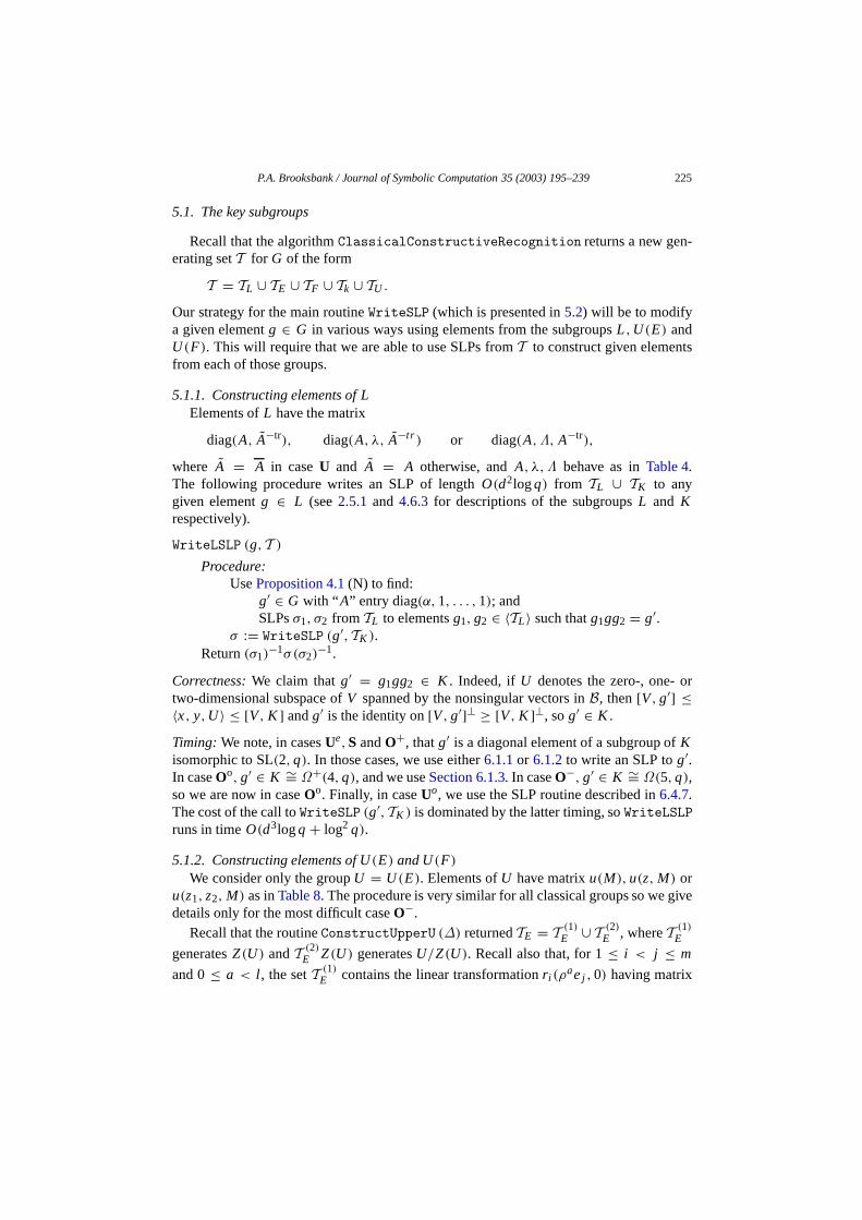
5.1. The key subgroups

Recall that the algorithmClassicalConstructiveRecognition returns a new gen-erating setT for G of the form

T = TL ∪ TE ∪ TF ∪ Tk ∪ TU .

Our strategy for the main routineWriteSLP (which is presented in5.2) will be to modifya given elementg ∈ G in various ways using elements from the subgroupsL,U(E) andU(F). This will require that we are able to use SLPs fromT to construct given elementsfrom each of those groups.

5.1.1. Constructing elements of LElements ofL have the matrix

diag(A, A−tr), diag(A, λ, A−tr ) or diag(A,Λ, A−tr),

where A = A in caseU and A = A otherwise, andA, λ,Λ behave as inTable 4.The following procedure writes an SLP of lengthO(d2logq) from TL ∪ TK to anygiven elementg ∈ L (see2.5.1 and 4.6.3 for descriptions of the subgroupsL and Krespectively).

WriteLSLP (g,T )Procedure:

UseProposition 4.1(N) to find:g′ ∈ G with “ A” entry diag(α,1, . . . ,1); andSLPsσ1, σ2 from TL to elementsg1, g2 ∈ 〈TL〉 such thatg1gg2 = g′.

σ := WriteSLP (g′,TK ).Return(σ1)

−1σ(σ2)−1.

Correctness:We claim thatg′ = g1gg2 ∈ K . Indeed, ifU denotes the zero-, one- ortwo-dimensional subspace ofV spanned by the nonsingular vectors inB, then[V, g′] ≤〈x, y,U〉 ≤ [V, K ] andg′ is the identity on[V, g′]⊥ ≥ [V, K ]⊥, sog′ ∈ K .

Timing: We note, in casesUe,S andO+, thatg′ is a diagonal element of a subgroup ofKisomorphic to SL(2,q). In those cases, we use either6.1.1or 6.1.2to write an SLP tog′.In caseOo, g′ ∈ K ∼= Ω+(4,q), and we useSection 6.1.3. In caseO−, g′ ∈ K ∼= Ω(5,q),so we are now in caseOo. Finally, in caseUo, we use the SLP routine described in6.4.7.The cost of the call toWriteSLP (g′,TK ) is dominated by the latter timing, soWriteLSLPruns in timeO(d3logq + log2 q).

5.1.2. Constructing elements of U(E) and U(F)We consider only the groupU = U(E). Elements ofU have matrixu(M),u(z,M) or

u(z1, z2,M) as inTable 8. The procedure is very similar for all classical groups so we givedetails only for the most difficult caseO−.

Recall that the routineConstructUpperU (∆) returnedTE = T (1)E ∪ T (2)

E , whereT (1)E

generatesZ(U) andT (2)E Z(U) generatesU/Z(U). Recall also that, for 1≤ i < j ≤ m

and 0≤ a < l , the setT (1)E contains the linear transformationr i (ρ

aej ,0) having matrix


u(0,0, Ei j (ρa)− Ej i (ρ

a)) ∈ Z(U). Hence, elements ofZ(U), relative toB, are also vec-

tors relative toT (1)E when viewed as elements of anFp-space of dimension<kd2 (cf. (†)).

The following procedure writes an SLP of lengthO(d2logq) from TE to any givenelementg ∈ U .

WriteUSLP (g,TE) [CaseO−]

Procedure:if (g ∈ Z(U)) then

Expressg as anFp-linear combination of the basisT (1)(†)E .

Hence return an SLP of lengthO(d2logq) from T (1)E to g.

else [g = u(z1, z2,M) f or z1, z2 ∈ Fm not both zero]

Write zs =∑mi=1

∑k−1a=0αiasεi (ρ

a)‡ for s = 1,2, where 0≤ αias < p.Hence, write an SLP of lengthO(dlogq) from T (2)

E to

h =2∏

s=1

m∏i=1

k−1∏a=0

r i (ρavs, λa,s)

αias .

Recursively setσ ′ := WriteUSLP (gh−1,TE); [gh−1 ∈ Z(U)]Returnσ ′σ .

(†) Performing even elementary linear algebra (such as a change of basis) in theO(kd2)-dimensional vector spaceZ(U) requiresO(k3d6) integer computations, soit is crucial that we constructed the exactFp-basisT (1)

E for Z(U) directly. Thisdimensional blow-up was also avoided inCeller (1997), but using different ideas.

(‡) The row vectorsεi (λ) are defined in (19).

Correctness:The only part of the procedure which needs justification is that the input tothe recursive call,gh−1, is in Z(U). This follows from the construction ofh. Indeed, ifg = u(z1, z2,M), thenh = u(z1, z2,M∗) for some matrixM∗, sogh−1 = u(0,0,M ′) ∈Z(U) for some matrixM ′.Timing:µ = O(d3logq) to computegh−1 since the elements ofT (2)

E are sparse.

5.2. The SLP algorithm

We now complete the proof ofTheorem 1.1for d ≥ 5. Let g ∈ GL(V) be given. Webegin with some preliminary checks to recognise wheng /∈ G. Compute det(g) and reportthatg /∈ G if this is not 1. Otherwise, verify thatg preserves theG-invariant form obtainedin 4.2and report thatg /∈ G if this is not the case. We are left with the possibility, in caseO, thatg ∈ SOε(V)\G. However, there are elementary tests to recognise when this is thecase(cf. Kleidman and Liebeck 1990,pp. 29–30), so we may now assume thatg ∈ G.

Our strategy is to use elements from the subgroupsU(E),U(F) andL to filter g downthe following short chain of subgroups:

G > GE > GE,F > 1;verifying the correctness of each filtration will usually just involve multiplying matrices.


Table 11Matrix entriesz, z1, z2,M (notation as in 2.5.2)

Case z M

S,O+,Ue Mtr = −A−1BOo,Uo z = ξ A−tr Mtr = −A−1B − ztrzO− zi = ξi A−tr Mtr = −A−1B − ztr

1 zσ(1) − αztr2 zσ(2)

Write g relative toB, so that

g =(

A BC D

),

( A ξ tr Bη λ ω

C ζ tr D

)or

A ξ tr1 ξ tr

2 Bη1 λ11 λ12 ω1η2 λ21 λ22 ω2C ζ tr

1 ζ tr2 D

as in (2) and(3) or (4) depending upon the type ofG. The following is a pseudo-codeoverview of the SLP algorithm.

WriteSLP (g,T )Procedure:(g′, σu1, σu2) := UpperReduce (g,T ), [5.2.1](g′′, σl ) := LowerReduce (g′,T ), and [5.2.2]σ := WriteLSLP (g′′,T ). [5.1.1]

Return(σu1)−1σ(σu2σl )

−1.

5.2.1. From G to GE

The following algorithm returns a triple(g′, σ1, σ2), whereg′ ∈ GE and, fori = 1,2,σi is an SLP of lengthO(d2logq) from T to an elementhi such thatg′ = h1gh2.

UpperReduce (g,T )Procedure:if (A is nonsingular)then

u := u(M), u(z,M) or u(z1, z2,M) in U(E) as inTable 11.w := utr.Return the triple (gw,1, WriteUSLP (w,T )). [5.1.2]

else [A is singular]r := rank(A).

UseProposition 4.1(S) to findg′ ∈ G with entry “A” of the form(Ar 00 0

), whereAr = diag(α1, . . . , αr ) for αi ∈ F

∗, together with SLPs

σi (i = 1,2) of lengthO(d2logq) from TL to elementsg1, g2 ∈ 〈TL〉such thatg1gg2 = g′.Recursively set(g′′,1, σ ) := UpperReduce (g′xr ,T ); [xr ∈ TU ]Return the triple(g′′, σ1, σ2xrσ).

Correctness:Suppose first thatA is nonsingular. Then it is an easy matter to verify thatthe entries ofu (Table 11) satisfy the appropriate constraints for an element ofU , and thenthatgw ∈ GE, as required.


Suppose then thatA is singular. We need to show thatg′xr has nonsingular “A” entry(so that we can make the recursive callUpperReduce (g′xr ,T )) and, in caseO+, thatm− r is even (since otherwisexr is undefined).

Write the top block entries ofg′ (corresponding to the firstm rows) as follows:(Ar 00 0

)(B11 B12B11 B12

),

(Ar 00 0

)(ξ tr1ξ tr2

)(B11 B12B21 B22

)or

(Ar 00 0

)(ξ tr11ξ tr12

)(ξ tr21ξ tr22

)(B11 B12B21 B22

),

so thatB12 is m× (m− r ), B22 is (m− r )× (m− r ), ξ12 ∈ Fm−r etc.

Claim 1. B21 = 0 in all cases;ξ2 = 0 in casesUo andOo; andξ12 = ξ22 = 0 in caseO−.

This technical fact is an elementary consequence of the matrix constraints imposed uponthesem rows ofg′ (cf. Tables 1and2). Again, we give details only for the most difficultcaseO−. We consider three different sets of constraints arising from the three differentpossible bases for the definite line〈v1, v2〉 (cf. Lemma 2.1).

Caseq ≡ 3 (mod 4). Sinceg′ preserves( , ), we obtain the constraints

ξ tr12ξ12 + ξ tr

22ξ22 = 0 and B21Atrr + ξ tr

12ξ11 + ξ tr22ξ21 = 0.

For nonzero row vectorsv = (vi ),w = (wi ) ∈ GF(q)m−r , vtrv + wtrw = 0 only ifv2

i = −w2i for 1 ≤ i ≤ m − r . This can occur only if−1 = and hence only if

q ≡ 1 (mod 4). Hence,ξ12 = ξ22 = 0 and this case follows.Case≡ 1 (mod4). This is similar to the preceding case. The constraints here can be

satisfied by nonzeroξ12, ξ22 only if −ρ = , which is the case if and only ifq ≡ 3 (mod 4).Caseq is even. Sinceg′ preserves ( , ), we obtain the constraints

(i) ξ tr12ξ22 + ξ tr

22ξ12 = 0; and(ii) B21Atr

r + ξ tr12ξ21 + ξ tr

22ξ11 = 0.

Sinceg′ also preservesϕ, we have the additional constraint

(iii) each diagonal entry ofα1ξtr12ξ12 + α2ξ

tr22ξ22 + ξ tr

12ξ22 is zero,

whereα1, α2 are as inLemma 2.1. Equation (i) requires that if bothξ12 andξ22 are nonzero,thenξ12 = λξ22 for someλ ∈ F. By (iii), the matrixξ tr

22ξ22[α1λ2 + λ + α2] has zeros on

its diagonal. Hence, eitherξ22 = 0 or λ is a root of the equationα1x2 + x + α2 = 0. Inthe latter caseλv1 + v2 is then a singular vector of the definite line〈v1, v2〉. Henceξ22 = 0and it follows from (iii) thatξ12 = 0 and then from (ii) thatB21 = 0.

Claim 2. g′xr has nonsingular “A” entry.

Using Claim 1 and the matrixxr (cf. 4.6.4) we see that the “A” entry of g′xr

is

(Ar ∗0 Am−r

), where Am−r = B22Mm−r . A corollary of Claim 1 is that B22 is

nonsingular (sinceg′ is nonsingular) and we showed in4.6.4that Mm−r is nonsingular.Hence,Am−r is nonsingular and the claim follows.


Table 12Matrix entriesz, z1, z2,M

Case z M

S,O+,Ue M = −D−1COo,Uo z = −ζ D−tr M = −D−1C − ztrz

z1 = −ζσ(1)D−tr

O−z2 = −α−1ζσ(1)D

−tr M = −D−1C − ztrσ(1)z1 − αztr

σ(2)z2

Claim 3. m− r is even in caseO+.

Sinceg′ ∈ G = Ω+(V) has “A” entry

(Ar 00 0

), it follows that dim(E ∩ F) = 0

and dim(Eg′ ∩ F) = m − r have the same parity (Kleidman and Liebeck, 1990, p. 30,description 4).

Claims 2and3 establish the correctness of the procedure.

Timing: O(d3logq), dominated byProposition 4.1.

5.2.2. From GE to GE,F

The following algorithm takes as input an elementg ∈ GE, and returns a pair(g′, σ ),whereg′ ∈ GE,F = L andσ is an SLP of lengthO(d2logq) from TE to an elementu ∈ U(E) such thatg′ = gu. Recall the notation for the block entries ofg in (2)–(4) andnote that:B = 0; ξ = 0 in casesOo andUo; andξ1 = ξ2 = 0 in caseO−.

LowerReduce (g,T )Procedure:

u := u(M), u(z,M) or u(z1, z2,M) in U(E) as inTable 12.Return the pair (gu, WriteUSLP (u,T )).

Correctness:SinceA is nonsingular, the constraints on the block matrix entries ofg meanthat A = D−tr in casesS andO andA = D

−trin caseU, soD is also nonsingular (hence

Table 12makes sense). Additionally, in casesOo andUo, we find thatω = 0 and, in caseO+, thatω1 = ω2 = 0. A matrix calculation shows thatgu ∈ GE,F .

Timing: O(d3logq).

5.2.3. Timing forWriteSLPAdding together the timing for each of its subroutines, we see thatWriteSLP returns an

SLP of lengthO(d2logq) fromT to any given elementg ∈ G in timeO(d3logq + log2 q).This completes the proof ofTheorem 1.1whend > 4.

6. Low dimensions

We now deal with the cases 2≤ d ≤ 4 and hence complete the proof ofTheorem 1.1.Our strategy will be to use the algorithm inConder and Leedham-Green (2001)forSL(2,q) subgroups to speed up the more time-consuming calculations. The algorithmsfor SU(3,q) and SU(4,q) (in 6.3and6.4respectively) are the most involved.


We assume that the elements of the generating setS are written relative to a standardbasis of the appropriate type. We alsoassume that q≥ 16 throughoutSection 6, sinceotherwise|G| is bounded and is handled by brute force.

6.1. Groups involving SL(2,q)

For each of the groupsG considered in6.1, we will first construct a functionθ : G →SL(2, r ) or SL(2, r )×SL(2, r ), wherer is eitherq orq2. The functionθ will be a procedurewhich takes any giveng ∈ G (not necessarily given as an SLP from the generators ofG)and computes its imagegθ . In each caseg → gθ (possibly modulo scalars) will be anisomorphism and we will be able to complete the recognition ofG by recognising SL(2,q)in its natural representation. For example, instead of writing an SLP fromS to the giveng ∈ G, we will instead write an SLP fromSθ to gθ , and then pull back toG.

6.1.1. The natural representationIn Conder and Leedham-Green (2001), a fast algorithm is presented which construc-

tively recognises a groupG = 〈S〉 ∼= SL(2,q), in its natural representation as a 2×2 matrixgroup with entries inF = GF(q), assuming an oracle to compute discrete logarithms inF∗. The algorithm constructs a generating seth, t1, t2 for G using SLPs fromS, where

(relative to a suitable basis)h is diagonal of orderq−1, andt1 (respectivelyt2) is an upper(respectively lower) unitriangular matrix (transvection).

The unique feature of the algorithm inConder and Leedham-Green (2001)is themethod employed to obtaint1 and t2. A direct search for a transvection would requireat leastq random choices to guarantee success with high probability, but this is avoidedby first findingh, and then usingh, together with discrete logarithms, to construct eachti .The number of random choices required then reduces dramatically toO(log logq).

Timing and reliability: O(ξ log logq + χ + logq) to construct the elementsh, t1 andt2.An SLP of lengthO(logq) from h, t1, t2 to any given elementg ∈ G is found usingO(logq) field operations. We assume (by repetition if necessary) that6.1.1succeeds withprobability>3/4.

6.1.2. SU(2,q)Since we need to work with the defining field GF(q2) in caseU it is convenient to have

a separate routine for SU(2,q) subgroups (reliability and timing will be as in6.1.1). LetG = 〈S〉 = SU(V), preserving an Hermitian form on the 2-spaceV overF = GF(q2),whose matrices are written relative to a standard basise, f .

The isomorphismθ (Taylor, 1992, Theorem10.9): useLemma 3.4(i) to find 0 = δ = −δand defineθ : SU(V)→ SL(V0), whereV0 is a 2-space overF0, sending(

a bc d

)→(

a bδc/δ d

).

6.1.3. Ω+(4,q)Let G = 〈S〉 = Ω+(V), preserving a quadratic formϕ = ϕ+ on the 4-spaceV . HereG

preserves a tensor decompositionV = U ⊗ W of V , which gives rise to a homomorphismθ : G → PSL(2,q)× PSL(2,q).


The homomorphismθ : We indicate two alternative methods for constructingθ ; the timingis dominated by6.1.1.

The first uses the quadratic formϕ and the fact thatG acts intransitively onthe set of 2(q + 1) t.s. lines of V , with two orbits Ol and Or of equal size(Kleidman and Liebeck, 1990, p. 30, description 4). Viewing each orbit as a projectiveline, we compute the action of any giveng ∈ G on each line, and hence obtaingθ .

The second uses the more general algorithm inLeedham-Green and O’Brien (1997)forcomputing tensor decompositions. Applied in the present setting, this is equivalent to theSMASH algorithm presented inHolt et al. (1996).

Completion:It is now fairly elementary to complete the recognition ofG. Let π1 andπ2denote the projections onto the SL(2,q) factors. We construct setsXi ⊂ G (i = 1,2)with 〈X1 ∪ X2〉 = G such that(Xi θ)π j = 1 if i = j and〈(Xi θ)πi 〉 = SL(2,q). This isachieved using two-element setsXi with one element of ppd#(p; k)-order and the other ofppd#(p; 2k)-order. Both sets are obtained, with high probability, by sampling at most 40elements ofG.

For example, the probability that a randomly chosen elementg ∈ G is such that(gθ)π1 has ppd#(p; k)-order such that(|(gθ)π1|, |(gθ)π2|) ≤ 2, is at least 1/8. For sucha g, gp(q+1) is selected as the ppd#(p; k)-element ofX1. Each of the other four types ofelement occur with similar probability. Hence, the probability that we fail to find at leastone of them after 40 tries is<4(1− 1/8)40 < 1/8.

6.1.4. Comments onΩ(3,q) andΩ−(4,q)Here, sinceΩ(3,q) ∼= SL(2,q) and Ω−(4,q) ∼= PSL(2,q2), we cite the algo-

rithm in Conder and Leedham-Green (2002)for recognising irreducible representationsof SL(2,q). We remark that, even thoughΩ−(4,q) was the most natural choice forK in 4.6.3, recognising this group usingConder and Leedham-Green (2002)would haverequired squaring the size of the given field; hence the choice ofΩ(5,q).

6.2. Sp(4,q)

Let G = 〈S〉 = Sp(V), preserving an alternating form on the 4-spaceV . Here, we willconstruct a homomorphismθ : G → Ω(5,q) and then use the main algorithm, applied toGθ , to complete the recognition ofG.

The homomorphismθ : Identify the exterior squareΛ2(V) with the 6-space of skew-symmetric 4× 4 matrices overF via u ∧ v := utrv − vtru ∈ W for u, v ∈ V . For

M =

0 x12 x13 x14−x12 0 x23 x24−x13 −x23 0 x34−x14 −x24 −x34 0

∈ Λ2(V),

defineϕ(M) := x12x34 − x13x24 + x14x23. Thenϕ is a quadratic form onΛ2(V). Set

M0 :=(

0 I−I 0

)∈ Λ2(V)


where I is the 2× 2 identity matrix. Observe that if matrices ofG and row vectorsof V are written relative to a fixed standard symplectic basise1,e2, f1, f2 of V , then(u, v) := uM0v

tr defines aG-invariant, alternating form onV . In particular,M0 is leftinvariant byG under the linear mapG → GL(Λ2(V)) sending(v → vg) → (MgtrMg).Hence, that map induces an action ofG on the quotient spaceW := Λ2(V)/〈M0〉 leavinginvariant(cf. Kleidman and Liebeck 1990,p. 45).

For a vectorM ∈ Λ2(V), let M = M〈M0〉 denote its image inW. Fix a basisM1, . . . ,M5 of the 5-spaceW and, for eachs ∈ S, compute the 5× 5 matrixsθ relativeto M1, . . . ,M5 representing the element of GL(W) induced bys on W under the mapM → StrMs. Thens → sθ defines the desired homomorphismθ : G → Ω(W).

Timing: O(ξ log logq + χ + log2 q) usingTheorem 1.1with d = 5.

6.3. SU(3,q)

Let G = 〈S〉 = SU(V), preserving an Hermitian form on the 3-spaceV . We begin ouralgorithm by constructing an SU(2,q) subgroup ofG.

6.3.1. FindingτExactly as inKantor (2001,6.6.1), choose up to 64 elementsτ of G in order to find one

of ppd#(p; 2k) · ppd#(p; k)- or ppd#(p; 2k) · ppd#(p; k) · ppd#(p; k/2)-order, respectively,depending on whetherk is odd or even; in addition we require that|τ2(q−1)| > 3 and, ifq is a Mersenne or Fermat prime, that 16 divides|τ |. Such aτ is found, with probability>1− 1/24, in time O(ξ + klog2 q).

6.3.2. Constructing LSeta := τ2(q−1) so thata is a ppd#(p; 2k)-element having ani -dimensional eigenspace

Vi for i = 1,2, whereV2 = V⊥1 . The following procedure usesa to construct a subgroup

L ∼= SU(2,q) of G.

Procedure:For up to 10 choicesg ∈ G, proceed as follows.

Setb := ag, A := 〈a,b〉 and useProposition 3.1to find L = 〈SL〉 = A′.For eachs ∈ SL , find a 2× 2 matrix s representing the element ofSU(2,q) induced bys on [V, L]; set L := 〈s | s ∈ SL〉.Use6.1.2to test whetherL ∼= SU(2,q) and, if so, to find a newgenerating setTL for L behaving as inTheorem 1.1for L, and stop.

ReturnA, L andTL if the latter has been found, or fail otherwise.

Correctness:If z is a point ofV2, let Vz denote the 2-space〈V1, z〉. For any giveng ∈ G,if Vg

1 = V1 thenVg1 lies on a unique lineVz for somez = z(g) ∈ V2. If z is singular, then

〈V1,Vg1 〉 = Vz has one-dimensional radicalz, and we will not succeed with that choice

of g. If z = Vg1 (i.e. if Vg

1 lies onV2 = V⊥1 ) then A ∼= 〈a〉 × 〈b〉 and we fail again for

suchg. Otherwise(Vg1 = z is nonsingular)A induces on the hyperbolic line〈V1,V

g1 〉

an irreducible subgroup of the general unitary group GU(2,q) generated by ppd#(p; 2k)elements of the same order. ByLemma 2.5, with probability>1/2, A′ ∼= SU(2,q) fixingthe nonsingular pointV2 ∩ Vg

2 = 〈V1,Vg1 〉τ . Hence, a fixed choiceb = ag gives rise to a

suitableA with probability>(1/2)·(1−q2(q+1)+q2−q+1/q2(q2−q+1)) > 0.46.


Timing: O(ξ log logq + log2 q + χ) dominated by the time for6.1.2andLemma 3.1.

Reliability: For a suitableA, Lemma 3.1correctly findsA′ with probability>1/2 and6.1.2correctly confirms thatL ∼= SU(2,q) with probability>3/4. Hence, a single conjugatebproduces a suitable generating setTL with probability>(3/8)(0.46) > 0.17. It followsthat at least one of our choices succeeds with probability>1− (0.83)10> 0.75.

6.3.3. Some elements of LTaking as input the subgroupL constructed in6.3.2, the next procedure returns a

standard basis ofV relative to which the elements ofL are easily recognised, togetherwith some elements ofL that we will use later in the algorithm.

Procedure:UseLemma 3.6to find a hyperbolic paire, f in the line[V, L].UseLemma 3.5to find 〈v〉 = [V, L]⊥.UseLemma 3.4(ii) to find α ∈ F

∗ s.t.αα = 1/(v, v); v := v/α.B := (e, v, f ) and write elements ofG relative toB.UseLemma 3.4(i) to find 0 = δ = −δ. Recalling thatζ generatesF∗

0,use6.1.2to construct thek + 2 elements

h :=(ζ 0 00 1 00 0 1/ζ

), r :=

( 0 0 δ

0 1 01/δ 0 0

), ti :=

( 1 0 00 1 0

ζ i−1δ 0 1

)

of L using SLPs of lengthO(logq) from TL , where 1≤ i ≤ k.Returnh, r , andt1, . . . , tk.

Timing:Dominated byO(klogq) for the construction of thek + 2 elements.Note thatT(〈e〉) = 〈ti | 1 ≤ i ≤ k〉; T(〈 f 〉) = T(〈e〉)r ; and 〈h〉 = NL (T(x)) ∩

NL (T(y)) has orderq − 1.

6.3.4. The subgroup QLet x = 〈e〉 andT = T(x). The following is a Las Vegas procedure for constructing a

generating setTQ for the groupQ = Op(Gx) of orderq3.

Procedure:for i ∈ 1,2

Choosegi ∈ G and setLi := 〈T, Trgi 〉.Use6.1.2(twice for eachi ) to test whether or notLi ∼= SU(2,q)and, if so, to constructhi ∈ NLi (T) ∩ NLi (T

rgi ) of orderq − 1.

ReturnTQ := t j , [h,hi ]h j−1 | i = 1,2,1 ≤ j ≤ k.Correctness and reliability:it suffices to show that〈TQ〉T/T = Q/T with highprobability. For fixedi , Li ∼= SU(2,q)with probability 1−1/(q3+1). As6.1.2is repeatedtwice for each choice, it will fail with probability<1/16 for suitablegi . Hence, we fail torecognise at least one SL(2,q)-subgroupLi with probability<21− 15(1− 1/q3)/16 <0.15. ForLi ∼= SL(2,q) (i = 1,2), [h,h1] and[h,h2] are in the same 1-space of the 2-spaceQ/T with probability 1/(q + 1) < 1/17. Ash induces onQ/T a scalar generatingF∗0, it follows that〈TQ〉T/T = Q/T with probability>1− 0.15+ 0.85/17 = 0.8.

Timing: O(ξ log logq + χ + logq) for the calls to6.1.2.


6.3.5. Algorithmic properties of QSince the Witt indexm is 1, we haveQ = U(x) (cf. 2.5.2), so elements ofQ(x) =

Op(Gx) have the form

u(λ, ν) =( 1 0 0λ 1 0ν −λ 1

),

whereλ, ν ∈ F are such thatν+ ν+ λλ = 0. The next result shows that we can efficientlyconstruct any given element ofQ.

Lemma 6.1. In time O(log2 q), one can find an SLP of length O(logq) from TQ to anygiven u= u(λ, ν) ∈ Q.

Proof. The 2k elements[h,hi ]h j−1(i = 1,2 and 1 ≤ j ≤ k) form an Fp-basis

for Q/T . Use linear algebra to find integers 0≤ αi j < p, and an elementu :=∏2i=1

∏kj=1([h,hi ]h j−1

)αi j , such thatu = u(−λ, ν′) for someν′ ∈ F. Hence write an

SLPσ of length O(logq) from TQ to u−1. Now use6.1.2to find integers 0≤ β j < p

for 1 ≤ j ≤ k such thatuu = ∏kj=1 t

β jj and write an SLPτ of length O(logq) from

ti | 1 ≤ i ≤ k to uu. Thenστ is the desired SLP.

By Theorem 2.1(vii), the subgroupQ acts regularly on the singular points ofV notequal tox. The following is an algorithmic version of this transitivity.

Lemma 6.2. Using only field operations, one can find the unique u∈ Q sending y to anygiven singular point z= x.

Proof. Let x = z = 〈ν, λ,1〉 be given, whereν + ν + λλ = 0. Thenu := u(−λ, ν) ∈ Q,and one easily checks that〈0,0,1〉u(−λ, ν) = 〈ν, λ,1〉.

6.3.6. Straight-line programsSetT := TQ ∪ (TQ)

r for the elementr constructed in6.3.3. The following is the three-dimensional version of the SLP algorithm described in5.2.

WriteSLP (g,T )Procedure:if (〈e〉g = 〈e〉) then

UseLemma 6.2to findw ∈ Qr such that〈e〉gw = 〈e〉.UseLemma 6.1to write an SLPσ1 from (TQ)

r tow.g := gw. [now g fixes〈e〉]

if (〈 f 〉g = 〈 f 〉) thenFindu ∈ Q such that〈 f 〉gu = 〈 f 〉.Write an SLPσ2 from TQ to u.g := gu. [now g fixes〈 f 〉]

For g = diag(λ, λq−1, λ−q) setγ := λδ.UseLemma 3.4(ii) to find η ∈ F

∗ s.t.ηη = −γ − γ q.


Use the equation

diag(λ, λq−1, λ−q) = u(ηγ−1, γ−q) · u(ηq, γ )tr · u(ηγ−q, γ−q) · r,

andLemma 6.1to write an SLPσ from TQ ∪ r to g.Return the SLPσ(σ1)

−1(σ2)−1.

Timing: O(log2 q), dominated byLemma 6.1.

6.3.7. Total timing and reliabilityConsidering the timing estimates of the subroutines in6.3.1through6.3.6, and adding

up the failure probabilities of the randomised subroutines, we obtain a suitableT , withprobability>1/2, in timeO(ξ log logq + χ + log2 q).

6.4. SU(4,q)

Let G = 〈S〉 = SU(V) preserving an Hermitian form on the 4-spaceV . The algorithmwe present for recognisingG has the same basic structure as that for SU(3,q) in 6.3. Wewill only give full details for a subroutine if there is no direct analogue in6.3.

6.4.1. FindingτProceed exactly as in6.3.1, this time choosing up to 48 elements ofG to find τ of

ppd#(p; 2k) · ppd#(p; 6k)-order. The timing and reliability are as in6.3.1.

6.4.2. Constructing LSet a := τq2−q+1, so that a is a ppd#(p; 2k)-element having ani -dimensional

eigenspace fori = 1,3 with V3 = V⊥1 . Now proceed exactly as in6.3.2to find A := 〈a,b〉,

L = 〈SL〉 := A′, and new generating setTL for the SL(2,q) subgroupL induced byL onVL = 〈V1,V

g1 〉. The timing and reliability are as in6.3.2.

6.4.3. Some elements of LAs in 6.3.3 we find a standard basisB, this time of the forme1,e2, f1, f2, where

〈e1, f1〉 = [V, L] andx = 〈e1〉 and y = 〈 f1〉 are the one-dimensional eigenspaces ofain V . This time we use6.1.2andTL just to construct generatorst1, . . . , tk for T := T(x),and the elementr which sendse1 → δ f1, f1 → e1/δ,e2 → e2 and f2 → f2.

6.4.4. The subgroup QWe use a slightly different approach to that in6.3.4to construct a generating setTQ for

the subgroupQ = Q(x) of orderq5.

Procedure:for i ∈ 1,2repeat (at most 12 times)

Choosegi ∈ G and setJi := 〈T, Tr , Tgi 〉;if ([V, Ji ] is a nonsingular 3-space)thenfor s a generator ofJi

s := element of SU(3,q) induced bys on [V, Ji ].Ji := 〈s | s a generator ofJi 〉.Use6.3to testJi ∼= SU(3,q); stop when suchJi is found.


if (J1 ∼= SU(3,q) ∼= J2 and[V, J1] = [V, J2]) thenTQi := generators forOp((Ji )x).ReturnTQ := TQ1 ∪ TQ2.

elseReport failure.

Correctness:For distinct SU(3,q) subgroupsJi of G, the groupsOp((Ji )x)/T are dis-tinct nonsingular 1-spaces of the two-dimensionalF-spaceQ/T , so Q = 〈Op((Ji )x) |i = 1,2〉.Timing: O(ξ log logq + χ + logq) for the≤24 calls to6.3.

Reliability: Sinceq ≥ 16, the probability that two SU(3,q) subgroups ofG are equalis small enough to be absorbed by our following (crude) estimates. ByLemma 2.6, forfixed i and fixed choicegi , Ji ∼= SU(3,q) with probability>1/2. For such aJi , thealgorithm6.3succeeds with probability>3/4. Thus a single choicegi produces a suitableJi with probability >(1/2)(3/4) > 1/4. Hence, the procedure fails with probability<(1− 1/4)12 + (1− 1/4)12< 2/e3.

6.4.5. Algorithmic properties of Q(x)There are versions ofLemmas 6.1 and 6.2for d = 4 (having the same timing) for

writing an SLP fromTQ to any given element ofQ and finding the unique element ofQ sending〈 f1〉 to any given〈 f ′〉 /∈ 〈e1〉⊥.

6.4.6. The generating setTWe do not follow the approach to SLPs taken in6.3.6, but rather use the general

algorithmWriteSLP presented inSection 5. Accordingly, we now tailor the generatingsetT to be consistent with the input to that algorithm.

Use6.3.6to construct an elementσ ∈ J1 of orderq2 − 1 normalisingT andT(〈 f1〉)and inducing the scalarρ on 〈e1〉 (henceρ−1 on 〈 f1〉). Also, construct using SLPs fromTQ ∪ r each of the 2k generators

T (1) := r1(ρi f2,0) | 0 ≤ i < 2k ⊂ Q

T (2)L := r ′

1(ρi e2,0) | 0 ≤ i < 2k ⊂ Qr

of the long root subgroupsR(e1, f2) andR( f1,e2) respectively (cf.(9)). ThenT (1)∪T (2)

is the generating set forL defined in(18). UseProposition 4.1to construct an elementc ∈ 〈TL〉 interchanging〈e1〉 and〈e2〉 and set

TE := TQ ∪ (TQ)c and TF := (TQ)

r ∪ (TQ)rc.

Finally, exactly as in4.6.4, construct the setTU and set

T := (T (1) ∪ T (2)) ∪ TE ∪ TF ∪ TL ∪ TU ,

exactly as in the main algorithm (but withTL replacingTK ).

Timing: O(ξ log logq + log2 q + χ) to construct the groupsR(e1, f2) and R( f1,e2) andfor the call to6.1.2.


Table 13Running times for input groupsΩ−(d,2k)

d10 20 30 40 50 60

24 4 4 6 11 18 2626 1 2 5 12 31 4728 1 2 4 11 20 57

q210 2 5 21 75 159 511212 4 7 34 75 212 430214 17 28 45 105 182 544

Table 14Running times for input groupsΩ−(d,3k)

d10 20 30 40 50 60

33 2 2 6 13 29 6434 2 2 6 15 45 8035 1 2 6 16 37 101

q36 2 4 23 61 245 58937 2 5 21 74 252 64638 4 9 35 97 328 583

6.4.7. Straight-line programsWe useWriteSLP (cf. Section 5) for caseU (d = 4) to write an SLP of lengthO(logq)

fromT to any given elementg ∈ G. Note that the algorithmWriteLSLP (cf. 5.1.1) reducesto the subgroup ofKe2, f2, which is our groupL.

6.4.8. Total timing and reliabilityA generating setT for G, behaving as inTheorem 1.1, is obtained with probability

>1− (1/4+ 2/e3) > 1/2, in timeO(ξ log logq + χ + log2 q).

7. Performance tests

The author has implemented the algorithm in the computer algebra systemGAP4(The GAP Group, 2000). Tables 13–15 show run-times (in seconds of CPU time, roundedto the nearest second) for a series of performance tests using the groupsΩ−(d,q).The stated timings are averages over 20 runs, obtained using an implementation ofThe GAP Group (2000)on a 2× PIII, 933 MHz, running RedHat Linux 7.1, 2.4.12 SMPkernel.

To illustrate the performance of our algorithm when handling large fields, wealso obtained a comparison with an implementation of Celler’s Sp(d,q) algorithm(Celler, 1997)which is available in theGAP3 share package “matrix”. The average termi-


Table 15Running times for input groupsΩ−(d, p)

d10 20 30 40 50 60

257 1 3 17 75 131 264p 6563 5 7 22 121 369 723

8191 9 9 27 92 332 889

Table 16Performance comparisons ford = 10 over fields of size 2i

Implementation 24 26 28 210 212

ClassicalConstructiveRecognition 9 5 5 11 20Sp(d,q) in “matrix” share package 2 7 21 137 656

nation times of the two implementations for 20 runs on a Sun UltraSPARC-II, 359 MHz,using a ten-dimensional group are summarised inTable 16.

Acknowledgements

The author would like to thank Bill Kantor for many helpful discussions during thepreparation of this manuscript, and Alexander Hulpke andAkos Seress for their adviceduring the implementation and testing of the algorithm. The suggestions for improvementprovided by both referees were also very much appreciated. This paper is based on part ofthe author’s Ph. D. dissertation (Brooksbank, 2001b, Constructive recognition of the finitesimple classical groups), completed under the direction of William Kantor. This researchwas supported, in part, by the National Science Foundation.

References

Babai, L., 1991. Local expansion of vertex-transitive graphs and random generation in finite groups.Proceedings of the ACM Symposium on Theory of Computing. pp. 164–174.

Brooksbank, P., 2001a. A constructive recognition algorithm for the matrix groupΩ(d,q). In: Kan-tor, W.M., Seress,A. (Eds.), Groups and Computation III, vol. 8. Ohio State University Math.Res. Inst. Publ.,Walter de Gruyter, Berlin, New York.

Brooksbank, P., 2001b. Constructive recognition of the finite simple classical groups. Ph. D. Thesis,U. Oregon.

Celler, F., 1997. Matrixgruppenalgorithmen inGAP. Ph. D. Thesis, RWTH Aachen.Celler, F., Leedham-Green, C.R., 1998. A constructive recognition algorithm for the special linear

group. The Atlas of Finite Groups: Ten Years On (Birmingham 1995), London MathematicalSociety Lecture Note Series, vol. 249.

Celler, F., Leedham-Green, C.R., Murray, S.H., Niemeyer, A.C., O’Brien, E.A., 1995. Generatingrandom elements of a finite group. Commun. Algebra 23, 4931–4948.


Conder, M., Leedham-Green, C.R., 2001. Fast recognition of classical groups over large fields.In: Kantor, W.M., Seress,A. (Eds.), Groups and Computation III, vol. 8. Ohio State UniversityMath. Res. Inst. Publ.,Walter de Gruyter, Berlin, New York.

Conder, M., Leedham-Green, C.R., O’Brien, E.A., 2002. Constructive recognition of SL(2,q) (inpreparation).

The GAP Group, 2000. Groups, Algorithms, and Programming, Version 4.2; Aachen, St Andrews.Available fromhttp://www-gap.dcs.st-and.ac.uk/gap.

Holt, D.F., Leedham-Green, C.R., O’Brien, E.A., Rees, S., 1996. Computing matrix group decom-positions with respect to a normal subgroup. J. Algebra 184, 795–817.

Holt, D.F., Rees, S., 1994. Testing modules for irreducibility. J. Aust. Math. Soc. (Ser. A) 57, 1–16.Kantor, W.M., Liebler, R.A., 1982. The rank 3 permutation representations of the finite classical

groups. TAMS 271, 1–71.Kantor, W.M., Seress,A., 2001. Black box classical groups. Mem. Amer. Math. Soc. 149 (708).Kleidman, P.B., Liebeck, M.W., 1990. The Subgroup Structure of the Finite Classical Groups. LMS

Lecture Note Series, vol. 129. Cambridge University Press, Cambridge, New York.Leedham-Green, C.R., 2001. The computational matrix group project. In: Kantor, W.M., Seress,A.

(Eds.), Groups and Computation III. Ohio State University Math. Res. Inst. Publ., vol. 8. Walterde Gruyter, Berlin, New York.

Leedham-Green, C.R., O’Brien, E.A., 1997. Recognising tensor products of matrix groups. Int. J.Algebra Comput. 7, 541–559.

Lidl, R., Niederreiter, H., 1983. Finite Fields, Encyclopedia of Mathematics and its Applications,vol. 20. Addison-Wesley.

Neumann, P.M., Praeger, C.E., 1992. A recognition algorithm for special linear groups. Proc. LondonMath. Soc. (3) 65, 555–603.

Niemeyer, A.C., Praeger, C.E., 1998. A recognition algorithm for classical groups over finite fields.Proc. London Math. Soc. (1) 77, 117–169.

Seress,A., 2002. Permutation Group Algorithms, Cambridge University Press (to appear).Taylor, D.E., 1992. The geometry of the classical groups. Heldermann, Berlin.Zsigmondy, K., 1892. Zur theorie der potenzreste. Monatsh. Math., Phys. 3, 265–284.

http://www-gap.dcs.st-and.ac.uk/gap

Documents

Constructive recognition of classical groups in their