Construction of initial vortex-surface fields and Clebsch potentials for flowswith high-symmetry using first integralsPengyu He and Yue Yang Citation: Physics of Fluids 28, 037101 (2016); doi: 10.1063/1.4943368 View online: http://dx.doi.org/10.1063/1.4943368 View Table of Contents: http://scitation.aip.org/content/aip/journal/pof2/28/3?ver=pdfcov Published by the AIP Publishing Articles you may be interested in Flow visualization of a vortex ring interaction with porous surfaces Phys. Fluids 24, 037103 (2012); 10.1063/1.3695377 Regimes of near-wall vortex dynamics in potential flow through gaps Phys. Fluids 20, 086605 (2008); 10.1063/1.2969471 Gliding arc in tornado using a reverse vortex flow Rev. Sci. Instrum. 76, 025110 (2005); 10.1063/1.1854215 Vortex ring pinchoff in the presence of simultaneously initiated uniform background co-flow Phys. Fluids 15, L49 (2003); 10.1063/1.1584436 Acoustic Energy Flow in High‐Symmetry Crystals J. Acoust. Soc. Am. 53, 1188 (1973); 10.1121/1.1913452

Reuse of AIP Publishing content is subject to the terms at: https://publishing.aip.org/authors/rights-and-permissions. Downloaded to IP:

162.105.227.139 On: Fri, 11 Mar 2016 02:35:53

PHYSICS OF FLUIDS 28, 037101 (2016)

Construction of initial vortex-surface fields and Clebschpotentials for flows with high-symmetry usingfirst integrals

Pengyu He1 and Yue Yang1,2,a)1State Key Laboratory for Turbulence and Complex Systems, College of Engineering,Peking University, Beijing 100871, China2Center for Applied Physics and Technology, Peking University, Beijing 100871, China

(Received 2 August 2015; accepted 23 February 2016; published online 10 March 2016)

We report a systematic study on the construction of the explicit, general form ofvortex-surface fields (VSFs) and Clebsch potentials in the initial fields with thezero helicity density and high symmetry. The construction methodology is basedon finding independent first integrals of the characteristic equation of a given three-dimensional velocity–vorticity field. In particular, we derive the analytical VSFsand Clebsch potentials for the initial field with the Kida–Pelz symmetry. Theseanalytical results can be useful for the evolution of VSFs to study vortical structuresin transitional flows. Moreover, the generality of the construction method is discussedwith the synthetic initial fields and the initial Taylor–Green field with multiplewavenumbers. C 2016 AIP Publishing LLC. [http://dx.doi.org/10.1063/1.4943368]

I. INTRODUCTION

Clebsch1 developed a Lagrangian formulation of the Eulerian velocity description for an incom-pressible inviscid flow. In the Clebsch representation, the incompressible fluid velocity at any timeinstant can be expressed, at least locally, in terms of three Clebsch potentials, and each vortex linecan be expressed locally by the intersection of iso-surfaces of the Clebsch potentials. More recently,the classical Clebsch representation has been extended to build Eulerian-Lagrangian frameworksfor Navier-Stokes dynamics,2–5 and it is considered as an appealing Hamiltonian formulation as acompromise between Eulerian and Lagrangian descriptions of fluid dynamics.6

Within the Clebsch representation,1,7 Yang and Pullin8 defined a vortex-surface field (VSF) asa scalar field φ(x, y, z) whose iso-surfaces are vortex surfaces. In a general sense, an open or closedvortex surface can be defined as a smooth surface or manifold embedded within a three-dimensionalvelocity field u(x, y, z), which has the property that the vorticity ω ≡ ∇ × u is tangent at every pointon the surface. The VSF should be a real function and globally smooth, so that it can be evolved usingits governing equation in numerical simulations and be extracted as level sets to show the geometryof vortex surfaces.

The VSF and Clebsch potentials have an inherent Lagrangian nature for visualizing and investi-gating vortical structures in fluid dynamics. The VSF, as a Lagrangian-based structure identificationmethod, is rooted in the Helmholtz vorticity theorem for inviscid flows,8 and a two-time approach wasintroduced as the numerical dissipative regularization for viscous flows.9,10 The VSFs for both initialTaylor–Green (TG)11,12 and Kida–Pelz (KP)13,14 velocity fields which display simple topology andhigh symmetry were constructed.8 Numerical results on the evolution of VSFs clarify the continuousvortex dynamics in viscous TG and KP flows including the vortex reconnection, rolling-up of vortextubes, vorticity intensification between anti-parallel vortex tubes, and vortex stretching and twisting.This suggests a possible scenario for explaining the transition from a smooth laminar flow to turbulentflow and scale cascade in terms of topology and geometry of vortex surfaces. Furthermore, the VSF isalso promising to be applied in transitional wall flows15 to elucidate the continuous temporal evolution

a)Electronic mail: yyg@pku.edu.cn

1070-6631/2016/28(3)/037101/13/$30.00 28, 037101-1 ©2016 AIP Publishing LLC

Reuse of AIP Publishing content is subject to the terms at: https://publishing.aip.org/authors/rights-and-permissions. Downloaded to IP:

162.105.227.139 On: Fri, 11 Mar 2016 02:35:53

037101-2 P. He and Y. Yang Phys. Fluids 28, 037101 (2016)

of vortical structures from a Lagrangian perspective. In particular, the VSF method can effectivelyidentify the vortex reconnection,16 which is a critical process for the scale cascade in transitions andis hard to be characterized via Eulerian-based vortex identification methods.17,18

Although the VSF has the potential for a paradigm of structure identification and tracking in fluidmechanics, there are open questions of its uniqueness, robustness, and computational feasibility.10,19

In particular, the existence of analytical VSFs and Clebsch potentials was rarely reported in the liter-ature,7,20,21 because challenges exist in the initial construction of VSFs and Clebsch potentials. Theanalytical Clebsch potentials for the TG initial field were obtained by solving the characteristic equa-tion of vorticity.22 A methodology based on the series expansion was developed8 to construct VSFsfor both TG and KP initial velocity fields, but only a numerical solution based on expansion of tailoredbasis functions was obtained for the KP flow.

In the present study, we derive the independent first integrals of the characteristic equation ofa given vorticity field. By using the first integrals, we demonstrate that the general, analytical formof VSFs and Clebsch potentials can be constructed for some given velocity–vorticity fields with thezero helicity density, e.g., the KP initial field and the TG initial field with multiple wavenumbers.These analytical results are new and can be useful as the initial conditions for the evolution of VSFsto study the generation and evolution of vortical structures in transitional flows.

We begin with introducing fundamentals of the first integral, VSF, and Clebsch potentials inSec. II. Then in Sec. III, we derive analytical VSFs for both TG and KP initial fields using firstintegrals. In Sec. IV, we develop a method to obtain the general form of Clebsch potentials. Someconclusions are drawn in Sec. V.

II. FIRST INTEGRAL, VSF, AND CLEBSCH POTENTIALS

In this section, the concept of the first integral, VSF, and Clebsch potentials will be firstreviewed, and then the relation between them will be discussed.

A. First integral

We consider the general form of nth-order ordinary differential equations (ODEs). Supposef i : Rn → R is a continuous function. Then for any initial value yi0 = (y10, y20, . . . , yn0) in Rn, thesystem

dyidx= f i(x, y1, . . . , yn), i = 1, . . . ,n (1)

must have a unique solution yi(x) = yi(x, yi0) with yi(0, yi0) = yi0. A function Φ : D ⊂ Rn → R iscalled a first integral of Eq. (1) in region D ⊂ Rn, when Φ is continuous together with its first partialderivatives, and Φ(y1(x), . . . , yn(x)) = constant is along the solution of Eq. (1) and is not constanton any open set in D. It is an open question if there exists a general method to find the global andnonconstant first integrals of Eq. (1), but the reward of finding these first integrals can be significantin the rare cases where they exist.23

B. VSF

Based on the definition, the constraint

ω · ∇φ = 0 (2)

for VSF8 is a first-order linear homogeneous partial differential equation (PDE). Consider a generalform of Eq. (2)

A1(x1, x2, . . . , xn) ∂Q∂x1+ · · · + An(x1, x2, . . . , xn) ∂Q

∂xn= 0, (3)

where x1, . . . , xn are independent variables, Q = Q(x1, . . . , xn) is an unknown function, and Ai ⊂ Dare known nontrivial functions. The characteristic equation of Eq. (3) is

dx1

A1(x1, x2, . . . , xn) =dx2

A2(x1, x2, . . . , xn) = · · · =dxn

An(x1, x2, . . . , xn) . (4)

Reuse of AIP Publishing content is subject to the terms at: https://publishing.aip.org/authors/rights-and-permissions. Downloaded to IP:

162.105.227.139 On: Fri, 11 Mar 2016 02:35:53

037101-3 P. He and Y. Yang Phys. Fluids 28, 037101 (2016)

From the theory of ODEs, it is necessary and sufficient that any solution Q(x1, x2, . . . , xn)of Eq. (3) is a first integral of Eq. (4). Since Eq. (4) contains n − 1 first integrals, namely,Φ1,Φ2, . . . ,Φn−1, the general solution of Eq. (3) can be expressed as Q = ψ(Φ1,Φ2, . . . ,Φn−1),where ψ : Rn−1 → R is an arbitrary continuously differentiable function.

In principle, one can obtain the numerical solution of Q by solving hyperbolic PDE (3). Nev-ertheless, it is shown that a necessary condition for the existence and uniqueness of solutions toequations of the type Eq. (3) is not satisfied.24 Therefore, the regular numerical approach, such asthe spectral method for solving Eq. (2) in a periodic domain, fails for the computation.8 Instead ofsolving Eq. (3) directly, we construct the general solution of Eq. (3) by finding the independent firstintegrals of Eq. (4).

Additionally, although the first integrals of ω satisfy the VSF constraint Eq. (2), they may havesingularities. Hence, a appropriate smooth function of the first integrals is required to carefullyremove the singularities.

C. Clebsch potentials

In the Clebsch representation,1 the incompressible fluid velocity at any time instant can beexpressed locally in terms of three scalar fields as

u = ϕ1∇ϕ2 − ∇ϕ3, (5)

where ϕ1 and ϕ2 are Clebsch potentials, and ϕ3 is used for the solenoidal projection. It follows thatthe vorticity can be expressed by

ω = ∇ϕ1 × ∇ϕ2. (6)

It is noted that both ϕ1 and ϕ2 satisfy the VSF constraint Eq. (2), but they may have singularities.8

From the vector analysis and Eq. (5), the vanishing helicity density

h ≡ u · ω = 0 (7)

is equivalent to (∇ϕ1 × ∇ϕ2) · ∇ϕ3 = 0 locally, which is also referred as the Frobenius condition ofintegrability. A velocity field with Eq. (7) everywhere, which is also called the complex-lamellarfield,25 can be expressed by Clebsch potentials globally as Eq. (5) where ϕ3 must be a first integralof ω or zero. On the other hand, the global existence of the Clebsch potentials in a control volumeΩ implies that the (total) helicity H ≡

Ω

h dΩ is vanishing within the volume whose boundary isa vortex surface.26 For the initial field with h , 0, global existence of the Clebsch potentials is notguaranteed, but it is still possible to find exact first integrals and VSFs in some particular flows, suchas the integrable Arnold–Beltrami–Childress flow.8,27

III. CONSTRUCTION OF INITIAL VSFS

In this section, we construct VSFs for a given vorticity field ω via finding first integrals of thecharacteristic equation of ω. First, we will apply this method to the initial TG field and compare theinitial VSFs with those obtained using the Fourier expansion method.8 Then, the proposed methodwill be applied to a challenging case, the initial KP field, in which only a numerical solution8 wasobtained using the series expansion method for solving Eq. (2).

A. Taylor-Green flow

The initial velocity field of the TG flow11,12 is

ux = ax sin x cos y cos z,uy = ay cos x sin y cos z,uz = az cos x cos y sin z,

(8)

where the parameters ax =2√3

sin(θ + 2π3 ), ay =

2√3

sin(θ − 2π3 ), and az =

2√3

sin θ with an arbitraryreal multiplicative constant of θ. The corresponding vorticity is

Reuse of AIP Publishing content is subject to the terms at: https://publishing.aip.org/authors/rights-and-permissions. Downloaded to IP:

162.105.227.139 On: Fri, 11 Mar 2016 02:35:53

037101-4 P. He and Y. Yang Phys. Fluids 28, 037101 (2016)

ωx = bx cos x sin y sin z,ωy = by sin x cos y sin z,ωz = bz sin x sin y cos z,

(9)

where bx = −(√

3 sin θ + cos θ), by = (√3 sin θ − cos θ), and bz = 2 cos θ.The characteristic equation of the vorticity field is

dxbx cos x sin y sin z

=dy

by sin x cos y sin z=

dzbz sin x sin y cos z

. (10)

From the first two terms, we obtain

by ln cos x = bx ln cos y + constant, (11)

and then

cosbyx/cosbx y = constant. (12)

Thus ΦTG1 = cosbyx/cosbx y is one of the first integrals of the initial TG vorticity field.

By repeating the manipulations above for the first term and the third term in Eq. (10), we obtainanother first integral ΦTG

2 = cosbx z/ cosbzx. The Jacobian matrix J(x, y, z) for ΦTG1 and ΦTG

2 hasRank(J) = 2, which implies that ΦTG

1 and ΦTG2 are two independent first integrals.

Then, the initial VSF φTG of the TG flow can be constructed from the first integrals in variousapproaches to remove singularities. For example, if bx ∈ N ,

φTG = ΦTG2 /ΦTG

1 = (cos x cos y cos z)bx, (13)

is a group of VSFs for the initial TG field. This initial VSF is similar to that developed using theFourier expansion method for the TG flow.8

Furthermore, for a general form of initial fields with TG symmetries and high wavenumbers,28

ux = ax sin mx cos ny cos pz,uy = ay cos mx sin ny cos pz,uz = az cos mx cos ny sin pz,

(14)

where m, n, and p are integers, we obtain the corresponding VSFs as

φTG = (cos mx cos ny cos pz)bx, (15)

where bx ∈ N .It is still an open question if there exists a general approach to find explicit first integrals or

VSFs for any given vorticity with h = 0 and perhaps under particular symmetries. A turbulent-likevelocity can involve Fourier modes with a range of wavenumbers rather than a small portion of lowwavenumbers in Eqs. (8) and (14). An attempt of finding first integrals and VSFs for the initial fieldwith TG symmetries and multiple wavenumbers is presented in Appendix A.

B. Kida-Pelz flow

The initial velocity field of the KP flow13,14 is defined as

ux = sin x(cos 3y cos z − cos y cos 3z),uy = sin y(cos 3z cos x − cos z cos 3x),uz = sin z(cos 3x cos y − cos x cos 3y).

(16)

The corresponding vorticity is

ωx = −2 cos 3x sin y sin z + 3 cos x(sin 3y sin z + sin y sin 3z),ωy = −2 cos 3y sin z sin x + 3 cos y(sin 3z sin x + sin z sin 3x),ωz = −2 cos 3z sin x sin y + 3 cos z(sin 3x sin y + sin x sin 3y),

(17)

and its characteristic equation is

Reuse of AIP Publishing content is subject to the terms at: https://publishing.aip.org/authors/rights-and-permissions. Downloaded to IP:

162.105.227.139 On: Fri, 11 Mar 2016 02:35:53

037101-5 P. He and Y. Yang Phys. Fluids 28, 037101 (2016)

dxωx=

dyωy=

dzωz. (18)

With the triple-angle formula, the first term in Eq. (18) becomes

dxωx=

d sin xωx cos x

=d sin x

(1 − sin2 x) sin y sin z(16 + 8sin2 x − 12sin2 y − 12sin2 z) . (19)

Similar manipulations are repeated for the other terms in Eq. (18) to re-express the equation only interms of sin x, sin y , and sin z.

By multiplying all the terms in Eq. (18) by 2 sin x sin y sin z, and setting α = cos2 x, β =cos2 y , and γ = cos2 z with the identity 1 − sin2 θ = cos2 θ, we can obtain

dαα(3β + 3γ − 2α) =

dββ(3γ + 3α − 2β) =

dγγ(3α + 3β − 2γ) . (20)

Thus characteristic equation (18) has been rewritten from a trigonometric form to a polynomialform in order to facilitate finding of the first integrals.

Note that Eq. (20) is homogeneous. By letting β = αU and γ = αV , it becomes

dαα2(3U + 3V − 2) =

αdU +Udαα2U(3 + 3V − 2U) =

V dα + αdVα2V (3 + 3U − 2V ) . (21)

From the first two terms of Eq. (21), after some algebra we obtain

dαα(3U + 3V − 2) =

dU5U − 5U2 . (22)

Similarly, applying the same change of variables from the first term and the third term in Eq. (21)yields

dαα(3U + 3V − 2) =

dV5V − 5V 2 . (23)

By comparing Eq. (22) with Eq. (23), we obtain an ODE of U and V

dU5U − 5U2 =

dV5V − 5V 2 , (24)

which can be solved as(U − 1)VU(V − 1) = C, (25)

where C is a constant independent with U and V . Hence, a first integral of Eq. (20) can be written as

ΦKP1 =

(U − 1)VU(V − 1) =

(α − β)γβ(α − γ) . (26)

Next, we seek another independent first integral of the KP initial field. From Eq. (25), U can bere-expressed by V and C as

U =V

V + C − CV. (27)

Substituting Eq. (27) into Eq. (23) yields

dαα=−2 + 3V (1 + 1/(V + C − CV ))

5V − 5V 2 dV, (28)

and its solution is

ln α = −45

ln(1 − V ) − 25

ln V +35

ln(CV − V − C) + constant. (29)

Then, substituting Eq. (25) into Eq. (29) with U = β/α and V = γ/α yields

β3(α − γ)4αγ

= constant. (30)

Therefore, we obtain another first integral of Eq. (18).

Reuse of AIP Publishing content is subject to the terms at: https://publishing.aip.org/authors/rights-and-permissions. Downloaded to IP:

162.105.227.139 On: Fri, 11 Mar 2016 02:35:53

037101-6 P. He and Y. Yang Phys. Fluids 28, 037101 (2016)

With α = cos2 x, β = cos2 y,γ = cos2 z, and extracting the square root, the final result of thefirst integrals of Eq. (20) is

ΦKP1 =

(cos2 y − cos2 x)cos2 z(cos2 z − cos2 x)cos2 y

, (31)

ΦKP2 =

cos3y(cos2 x − cos2 z)2cos x cos z

. (32)

The Jacobian matrix J(x, y, z) for ΦKP1 and ΦKP

2 has Rank(J) = 2, so ΦKP1 and ΦKP

2 are independent.According to the rotational symmetry of the KP flow, we obtain three groups of first integrals

ΦKP11 =

(cos2 y − cos2 x)cos2 z(cos2 z − cos2 x)cos2 y

, ΦKP21 =

cos3y(cos2 x − cos2 z)2cos x cos z

, (33)

ΦKP12 =

(cos2 z − cos2 y)cos2 x(cos2 x − cos2 y)cos2 z

, ΦKP22 =

cos3z(cos2 y − cos2 x)2cos y cos x

, (34)

ΦKP13 =

(cos2 x − cos2 z)cos2 y

(cos2 y − cos2 z)cos2 x, Φ

KP23 =

cos3x(cos2 z − cos2 y)2cos z cos y

. (35)

From the results above, we also construct nontrivial, globally smooth VSFs φKP for the KP initialfield. For example, the simplest one is

φKP = ΦKP11 Φ

KP12 Φ

KP13 Φ

KP21 Φ

KP22 Φ

KP23

= cos x cos y cos z(cos2 x − cos2 y)2(cos2 y − cos2 z)2(cos2 z − cos2 x)2. (36)

The iso-surfaces of φKP in the initial KP field are shown in Fig. 1 within a subdomain−π/2 ≤ x ≤ π/2 and 0 ≤ y, z ≤ π. Some vortex lines are integrated and plotted on the vortex sur-faces. We remark that the geometry of this explicit initial VSF is very similar to the numericalsolution.8,9

The particular initial VSF in Eq. (36) implies a general form of VSFs for the initial KP field

φKP = Acosaxcosbycoscz(cos2 x − cos2 y) a+b+2c2 (cos2 y − cos2 z) 2a+b+c

2 (cos2 z − cos2 x) a+2b+c2 ,

(37)

where A is an arbitrary real number and the parameters a,b,c, 2a+b+c2 , a+2b+c

2 , a+b+2c2 ∈ N , which

can be verified by Eq. (2).

FIG. 1. Iso-surfaces of the VSF in Eq. (36) at φKP= 0.002 (blue) and φKP=−0.002 (yellow) in the initial KP field. Somevortex lines are integrated and plotted on the vortex surfaces.

Reuse of AIP Publishing content is subject to the terms at: https://publishing.aip.org/authors/rights-and-permissions. Downloaded to IP:

162.105.227.139 On: Fri, 11 Mar 2016 02:35:53

037101-7 P. He and Y. Yang Phys. Fluids 28, 037101 (2016)

IV. CONSTRUCTION OF CLEBSCH POTENTIALS

A. Construction of Clebsch potentials using first integrals

The explicit Clebsch potentials can be constructed from multiple independent VSFs or firstintegrals, if the latter exist, for a given velocity field, and this approach has been successfullyapplied to the TG initial field.8

Given two known independent first integrals Φ1 and Φ2 of ω, the two vectors ω and ∇Φ1 × ∇Φ2are colinear. Assume they point in the same direction as

ω = µ(∇Φ1 × ∇Φ2). (38)

Here, the scalar

µ = |ω |/|∇Φ1 × ∇Φ2| (39)

is also a first integral of ω, which is proved in Appendix B.To seek particular Clebsch potentials, we rewrite Eq. (38) in the form of

ω = µ(∇Φ1 × ∇Φ2) = ∇(µΦ1) × ∇Φ2 − Φ1(∇µ × ∇Φ2) (40)

without loss of generality. In the special cases with ∇µ × ∇Φ2 = 0, e.g., µ is a constant, we cansimply construct the particular Clebsch potentials as ϕ1 = µΦ1 and ϕ2 = Φ2. In the general caseswith ∇µ × ∇Φ2 , 0, we have to seek a particular scalar ν that satisfies

ω = ∇(νΦ1) × ∇Φ2 = ν ∇Φ1 × ∇Φ2 + Φ1∇ν × ∇Φ2 (41)

and is a first integral of ω. If ν can be solved from Eq. (41), the corresponding Clebsch potentialsare ϕ1 = νΦ1 and ϕ2 = Φ2.

B. Construction of Clebsch potentials for the KP initial field

The analytical Clebsch potentials for the simple TG initial field Equation (8) have been devel-oped,22 but those for the relatively sophisticated cases, e.g., the KP initial field Equation (16) and theTG initial field with multiple wavenumbers (Eq. (14)), are still unknown. In this subsection, we willconstruct the explicit Clebsch potentials from multiple independent first integrals of the initial KPfield obtained in Sec. III B.

For the initial KP field with Eqs. (31) and (32), the scalar µ in Eq. (39) is reduced to a constantas µ = 2. By setting ϕKP

1 = µ1ΦKP1 and ϕKP

2 = µ2ΦKP2 with µ1µ2 = µ for constants µ1 and µ2, we

obtain two particular Clebsch potentials

ϕKP1 = µ1

(cos2 y − cos2 x)cos2 z(cos2 z − cos2 x)cos2 y

, (42)

ϕKP2 = µ2

cos3y(cos2 x − cos2 z)2cos x cos z

(43)

satisfying Eq. (6) for the initial KP field. The typical iso-surfaces of ϕKP1 and ϕKP

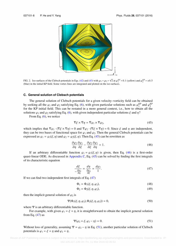
1 in the initial KPfield are shown in Fig. 2 within a subdomain 0 ≤ x, y, z ≤ π. The geometry of vortex lines can beexpressed by the intersections of the iso-surfaces.

It is straightforward to obtain the irrotational Clebsch potential ϕKP3 = 0 from Eq. (5) with the

particular solutions ϕKP1 and ϕKP

2 . Finally, the initial KP velocity can be expressed by the Clebschpotentials as

u = ϕKP1 ∇ϕ

KP2 . (44)

As an additional note, the analytical Clebsch potentials ϕ1 and ϕ2 given in Sec. 7 in Ref. 5 havethe similar form of Eq. (43) but they are incorrect. They fail to satisfy the definition of Clebschpotentials Eq. (5) and their derivation was omitted.

We remark that in general cases where µ is not constant, the construction of Clebsch potentialsby solving Eq. (41) may be challenging. For example, Appendix A presents the construction ofClebsch potentials with the non-constant µ in the TG initial field with multiple wavenumbers.

Reuse of AIP Publishing content is subject to the terms at: https://publishing.aip.org/authors/rights-and-permissions. Downloaded to IP:

162.105.227.139 On: Fri, 11 Mar 2016 02:35:53

037101-8 P. He and Y. Yang Phys. Fluids 28, 037101 (2016)

FIG. 2. Iso-surfaces of the Clebsch potentials in Eqs. (42) and (43) with µ1= µ2=√

2 at ϕKP1 = 0.1 (yellow) and ϕKP

2 =±0.5(blue) in the initial KP field. Some vortex lines are integrated and plotted on the iso-surfaces.

C. General solution of Clebsch potentials

The general solution of Clebsch potentials for a given velocity–vorticity field can be obtainedby seeking all the ϕ1 and ϕ2 satisfying Eq. (6), with given particular solutions such as ϕKP

1 and ϕKP2

for the KP initial field. This can be restated in a more general context, i.e., how to obtain all thesolutions ϕ1 and ϕ2 satisfying Eq. (6), with given independent particular solutions ξ and η?

From Eq. (6), we notice

∇ξ × ∇η = ∇ϕ1 × ∇ϕ2, (45)

which implies that ∇ϕ1 · (∇ξ × ∇η) = 0 and ∇ϕ2 · (∇ξ × ∇η) = 0. Since ξ and η are independent,they can be two bases of functional space for ϕ1 and ϕ2. Then the general Clebsch potentials can beexpressed as ϕ1 = ϕ1(ξ,η) and ϕ2 = ϕ2(ξ,η). Then Eq. (45) can be rewritten as

∂ϕ2

∂η

∂ϕ1

∂ξ− ∂ϕ2

∂ξ

∂ϕ1

∂η= 1. (46)

If an arbitrary differentiable function ϕ1 = ϕ1(ξ,η) is given, then Eq. (46) is a first-orderquasi-linear ODE. As discussed in Appendix C, Eq. (45) can be solved by finding the first integralsof its characteristic equation

dξ

− ∂ϕ1∂η

=dη∂ϕ1∂ξ

=dϕ2

1. (47)

If we can find two independent first integrals of Eq. (47)

Φ1 = Φ1(ξ,η,ϕ2), (48)Φ2 = Φ2(ξ,η,ϕ2), (49)

then the implicit general solution of ϕ2 is

Ψ(Φ1(ξ,η,ϕ2),Φ2(ξ,η,ϕ2)) = 0, (50)

where Ψ is an arbitrary differentiable function.For example, with given ϕ1 = ξ + η, it is straightforward to obtain the implicit general solution

from Eq. (47) as

Ψ(ϕ2 + ξ,ϕ2 − η) = 0. (51)

Without loss of generality, assuming Ψ = ϕ2 − η in Eq. (51), another particular solution of Clebschpotentials is ϕ1 = ξ + η and ϕ2 = η.

Reuse of AIP Publishing content is subject to the terms at: https://publishing.aip.org/authors/rights-and-permissions. Downloaded to IP:

162.105.227.139 On: Fri, 11 Mar 2016 02:35:53

037101-9 P. He and Y. Yang Phys. Fluids 28, 037101 (2016)

D. VSFs and Clebsch potentials for synthetic initial fields

We have demonstrated how to obtain the VSFs and Clebsch potentials for several givenvelocity–vorticity fields including the well-known TG and KP initial fields. In order to investigatethe generality of this technique in more initial fields, a synthetic vorticity field ωϑ, where the VSFand Clebsch potentials exist, can be constructed from a given smooth scalar field ϑ as

ωϑ = ∇ϑ × ∇ϑ0, (52)

where ϑ0 is an arbitrary scalar function. Consequently ϑ is the VSF of ωϑ from the identity(∇ϑ × ∇ϑ0) · ∇ϑ = 0. Additionally, ϑ and ϑ0 can be considered as a pair of Clebsch potentials forωϑ.

As an example, we use ϑ = sin x + sin y + sin z and ϑ0 = cos x + cos y + cos z to construct aninitial vorticity field

ωϑ = (sin(y − z),sin(z − x),sin(x − y)) (53)

from Eq. (52). This initial field was proposed by Ohkitani5 to study an Euler flow evolution with avery weak energy transfer.

On the other hand, assuming we do not know ϑ and ϑ0 a priori, we can solve the VSF andClebsch potentials by finding the first integrals of ωϑ. The characteristic equation of Eq. (53) is

dxsin(y − z) =

dysin(z − x) =

dzsin(x − y) , (54)

and it can be re-expressed as

cos x dxcos x sin(y − z) =

cos y dycos y sin(z − x) =

cos z dzcos z sin(x − y) . (55)

Applying Componendo and the trigonometric identity

cos x sin(y − z) + cos y sin(z − x) + cos z sin(x − y) = 0 (56)

in Eq. (55) yields

cos x dx + cos y dy + cos z dz = d(sin x + sin y + sin z) = 0, (57)

which shows that ϑOh1 = sin x + sin y + sin z is a first integral for Eq. (54). Using the similar proce-

dure, we can derive another first integral ϑOh2 = cos x + cos y + cos z, then we obtain the VSF and

Clebsch potentials for Eq. (53) using first integrals.Although there appears to be no general technique of solving first integrals, the method of

first integrals has been applied successfully in several given initial velocity–vorticity fields. Ageneralized method is expected to solve the first integrals of Eq. (3) numerically, though it canbe challenging to develop a suitable regularization method owing to the existence and uniquenessissues8,24 of solutions of Eq. (3). The TG and KP initial fields with the known, explicit first integralscan be good candidates to verify the proposed numerical methods.

Besides these fields with high-symmetry, a more challenging verification case can be devel-oped using a synthetic initial vorticity field ωϑ generated from a turbulent-like scalar field ϑ. Forexample, the synthetic vorticity field can be generated as

ωϑ =

(∂ϑ

∂ y− ∂ϑ∂z,∂ϑ

∂z− ∂ϑ∂x

,∂ϑ

∂x− ∂ϑ∂ y

), (58)

with a simple nontrivial ϑ0 = (x, y, z).

V. CONCLUSIONS

We report a systematic study on the construction of VSFs and Clebsch potentials for giveninitial three-dimensional velocity–vorticity fields with high-symmetry. Instead of solving the PDEfor the VSF constraint directly,8 we seek the first integrals of the characteristic equation of vorticity.

Reuse of AIP Publishing content is subject to the terms at: https://publishing.aip.org/authors/rights-and-permissions. Downloaded to IP:

162.105.227.139 On: Fri, 11 Mar 2016 02:35:53

037101-10 P. He and Y. Yang Phys. Fluids 28, 037101 (2016)

Then the initial VSFs and Clebsch potentials can be constructed from the first integrals. In addi-tion, the implicit form of the general solution, relying on an arbitrary continuously differentiablefunction, can be obtained from a group of particular solutions of VSFs and Clebsch potentials.Particularly, we derive the explicit general forms of VSFs and Clebsch potentials for the KP initialfield and for the TG initial field with multiple wavenumbers.

This methodology based on first integrals can be applicable to obtain explicit VSFs and Cleb-sch potentials in other flows with high-symmetry and the zero helicity density, though ad hocmethods may be required to manipulate the characteristic equation to solve first integrals. Theseanalytical VSFs and Clebsch potentials can be valuable for further investigations on the Lagrangianvortex dynamics via their temporal evolution, particularly in inviscid flows5 and in viscous transi-tional flows,9,10 and for the development of the general numerical methods of solving VSFs from anarbitrary velocity field as benchmark solutions.

ACKNOWLEDGMENTS

The authors thank D. I. Pullin, W.-D. Su, and S. Xiong for helpful comments. This workhas been supported in part by the National Natural Science Foundation of China (Nos. 11342011,11472015, and 11522215) and the Thousand Young Talents Program of China.

APPENDIX A: INITIAL FIELD WITH TG SYMMETRIES AND MULTIPLE WAVENUMBERS

The generalized Fourier representation12 of velocity in the evolution of the TG flow is

ux =

∞m=0

∞n=0

∞p=0

ux sin mx cos ny cos pz,

uy =

∞m=0

∞n=0

∞p=0

uy cos mx sin ny cos pz,

uz =

∞m=0

∞n=0

∞p=0

uz cos mx cos ny sin pz,

(A1)

where ux, uy, and uz are Fourier coefficients under constraints of TG symmetries. The explicit VSFsof the generalized TG field may exist and valuable, but it appears to be challenging to solve themfrom Eq. (A1) with infinite wavenumbers. As an attempt to solve first integrals of a velocity fieldwith multiple wavenumbers, we set fixed m and n, and equal coefficients as ux = uy = uz = 1. ThenEq. (A1) is reduced to a solvable case as

ux = sin mx cos nypl=1

cos l z = sin mx cos ny *,

sin (2p+1)z2 − sin z

2

2 sin z2

+-,

uy = cos mx sin nypl=1

cos l z = sin mx cos ny *,

sin (2p+1)z2 − sin z

2

2 sin z2

+-,

uz = cos mx cos nypl=1

sin l z = sin mx cos ny *,

cos z2 − cos (2p+1)z

2

2 sin z2

+-,

(A2)

where p is an arbitrary positive integer or p → ∞, and the helicity density of Eq. (A2) is vanishing.The characteristic equation of the vorticity field of Eq. (A2) is

− 2 tan mx dx

2n cos z2 + (1 − 2n + 2p) cos (2p+1)z

2 − cot z2 sin (2p+1)z

2

=2 tan ny dy

2m cos z2 + (1 − 2m + 2p) cos (2p+1)z

2 − cot z2 sin (2p+1)z

2

=dz

(m − n)(sin z2 − sin (2p+1)z

2 ) , (A3)

Reuse of AIP Publishing content is subject to the terms at: https://publishing.aip.org/authors/rights-and-permissions. Downloaded to IP:

162.105.227.139 On: Fri, 11 Mar 2016 02:35:53

037101-11 P. He and Y. Yang Phys. Fluids 28, 037101 (2016)

which is equivalent to two variable separable ODEs

tan mx dx =2n cos z

2 + (1 − 2n + 2p) cos (2p+1)z2 − cot z

2 sin (2p+1)z2

−2(m − n) sin z2 − sin (2p+1)z

2

dz, (A4)

tan ny dy =2m cos z

2 + (1 − 2m + 2p) cos (2p+1)z2 − cot z

2 sin (2p+1)z2

2(m − n) sin z2 − sin (2p+1)z

2

dz. (A5)

Two independent first integrals of Eq. (A3) can be solved directly as

ΦTGM1 = cos−(m−n)(1+p)mx cosm(−1+2n−p) (1 + p)z

2sinm(1+p) z

2sin−m(1+p) pz

2, (A6)

ΦTGM2 = cos(m−n)(1+p)ny cosn(−1+2m−p) (1 + p)z

2sinn(1+p) z

2sin−n(1+p)

pz2. (A7)

Then the VSF for can be constructed as

φTGM = *,

ΦTGM1

ΦTGM2

+-

(m−n)(1+p)= cos mx cos ny cos

(1 + p)z2

sinpz2

cscz2, (A8)

which only has removable singularities. This VSF in Eq. (A8) is distinguished with the TG VSFsEqs. (13) and (14) because Eq. (A8) has multiple characteristic scales. In other words, the corre-sponding vortex surfaces, as iso-surfaces of Eq. (A8) with a single iso-contour value, have differentsizes. For example, the iso-surfaces of φTGM in Eq. (A8) with m = 1, n = 2, and p = 4 is shown inFig. 3 within a subdomain −π/2 ≤ x ≤ π/2, −π/4 ≤ y ≤ π/4, and −π ≤ z ≤ π. Some vortex linesare integrated and plotted on the vortex surfaces. It is expected to obtain the explicit VSF of a morecomplex, or perhaps turbulent-like field in future work.

Based on the independent first integrals φTGM and ΦTGM1 , we constructed the Clebsch potentials

for Eq. (A2) by solving ν from Eq. (41) as

ω = ν ∇φTGM × ∇ΦTGM1 + φTGM∇ν × ∇ΦTGM

1 . (A9)

We obtain the solution

ν =

(cos(m−n)(1+p)mx cosm(1−2n+p) (1 + p)z

2sin1−m(1+p) z

2

sinm(1+p) pz2

(−2n cos

z2+ (2n − 1 − 2p) cos

1 + p2

z + cotz2

sin1 + p

2z) )

(2mn(1 + p)

(p cos

pz2

cos(1 + p)z

2sin

z2

− sinpz2

(cos

z2

cos(1 + p)z

2+ (1 − 2n + p) sin

z2

sin(1 + p)z

2

))), (A10)

FIG. 3. Iso-surfaces of the VSF in Eq. (A8) with m = 1, n = 2, and p = 4 at φTGM = 0.5 (blue) and φTGM =−0.5 (yellow)present different characteristic scales of the vortex surfaces in the initial TG field. Some vortex lines are integrated and plottedon the vortex surfaces.

Reuse of AIP Publishing content is subject to the terms at: https://publishing.aip.org/authors/rights-and-permissions. Downloaded to IP:

162.105.227.139 On: Fri, 11 Mar 2016 02:35:53

037101-12 P. He and Y. Yang Phys. Fluids 28, 037101 (2016)

where the derivation is omitted. Thus, the corresponding particular Clebsch potentials are ϕTGM1 =

νφTGM and ϕTGM2 = ΦTGM

1 .

APPENDIX B: PROOF OF µ AS A FIRST INTEGRAL OF VORTICITY

It is interesting that a nontrivial µ in Eq. (39) is also a first integral of vorticity ω. FromEq. (38), we obtain

1µ=

1ωx

(∂Φ1

∂ y

∂Φ2

∂z− ∂Φ1

∂z∂Φ2

∂ y

)=

1ωy

(∂Φ1

∂z∂Φ2

∂x− ∂Φ1

∂x∂Φ2

∂z

)=

1ωz

(∂Φ1

∂x∂Φ2

∂ y− ∂Φ1

∂ y

∂Φ2

∂x

),

(B1)

which implies

ωx∂µ

∂x= −µ2

(∂2Φ1

∂x∂ y∂Φ2

∂z+∂2Φ2

∂x∂z∂Φ1

∂ y− ∂2Φ1

∂x∂z∂Φ2

∂ y− ∂2Φ2

∂ y∂z∂Φ1

∂x

)+ µ

∂ωx

∂x. (B2)

This is the first term of ω · ∇µ, and other two terms ωy∂µ∂y

and ωz∂µ∂z

have the similar form. Thesummation of the three terms results in that the first term in the right hand side of Eq. (B2) iscanceled, and then yields

ω · ∇µ = µ(∂ωx

∂x+∂ωy

∂ y+∂ωz

∂z

)= µ (∇ · ω) = 0. (B3)

Hence, µ is a first integral of ω.

APPENDIX C: FIRST-ORDER QUASI-LINEAR PARTIAL DIFFERENTIAL EQUATION

We consider a first-order quasi-linear PDE

A1(x1, x2, . . . , xn,Q) ∂Q∂x1+ · · · + An(x1, x2, . . . , xn,Q) ∂Q

∂xn= R(x1, x2, . . . , xn,Q), (C1)

where Ai and R are known, continuously differentiable functions in D. Solving Eq. (C1) is similarto solving Eq. (3). The characteristic equation of Eq. (C1) is

dx1

A1(x1, x2, . . . , xn,Q) = · · · =dxn

An(x1, x2, . . . , xn,Q) =dQ

R(x1, x2, . . . , xn,Q) . (C2)

Suppose n independent first integrals of Eq. (C2) are

Φ1(x1, x2, . . . , xn,Q), . . . ,Φn(x1, x2, . . . , xn,Q) (C3)

and ψ : Rn → R is an arbitrary continuously differentiable function. Then

ψ(Φ1(x1, x2, . . . , xn,Q), . . . ,Φn(x1, x2, . . . , xn,Q)) = 0 (C4)

is the implicit general solution of Eq. (C2).

1 A. Clebsch, “Ueber die integration der hydrodynamischen gleichungen,” J. Reine Angew. Math. 56, 1–10 (1859).2 P. Constantin, “An Eulerian–Lagrangian approach to the Navier–Stokes equations,” Commun. Math. Phys. 216, 663–686

(2001).3 K. Ohkitani and P. Constantin, “Numerical study of the Eulerian–Lagrangian formulation of the Navier-Stokes equations,”

Phys. Fluids 15, 3251–3254 (2003).4 C. Cartes, M. D. Bustamante, and M. E. Brachet, “Generalized Eulerian–Lagrangian description of Navier–Stokes dy-

namics,” Phys. Fluids 19, 077101 (2007).5 K. Ohkitani, “A geometrical study of 3D incompressible Euler flows with Clebsch potentials—A long-lived Euler flow and

its power-law energy spectrum,” Physica D 237, 2020–2027 (2008).6 R. Salmon, “Hamiltonian fluid mechanics,” Annu. Rev. Fluid Mech. 20, 225–256 (1988).7 H. Lamb, Hydrodynamics, 6th ed. (Cambridge University Press, 1932).8 Y. Yang and D. I. Pullin, “On Lagrangian and vortex-surface fields for flows with Taylor–Green and Kida–Pelz initial

conditions,” J. Fluid Mech. 661, 446–481 (2010).

Reuse of AIP Publishing content is subject to the terms at: https://publishing.aip.org/authors/rights-and-permissions. Downloaded to IP:

162.105.227.139 On: Fri, 11 Mar 2016 02:35:53

037101-13 P. He and Y. Yang Phys. Fluids 28, 037101 (2016)

9 Y. Yang and D. I. Pullin, “Evolution of vortex-surface fields in viscous Taylor-Green and Kida-Pelz flows,” J. Fluid Mech.685, 146–164 (2011).

10 D. I. Pullin and Y. Yang, “Whither vortex tubes?,” Fluid Dyn. Res. 46, 061418 (2014).11 G. I. Taylor and A. E. Green, “Mechanism of the production of small eddies from large ones,” Proc. R. Soc. A 158, 499–521

(1937).12 M. E. Brachet, D. I. Meiron, S. A. Orszag, B. G. Nickel, R. H. Morf, and U. Frisch, “Small-scale structure of the Taylor–Green

vortex,” J. Fluid Mech. 130, 411–452 (1983).13 S. Kida, “Three-dimensional periodic flows with high-symmetry,” J. Phys. Soc. Jpn. 54, 2132–2136 (1985).14 O. N. Boratav and R. B. Pelz, “Direct numerical simulation of transition to turbulence from a high-symmetry initial condi-

tion,” Phys. Fluids 6, 2757–2784 (1994).15 Y. Zhao, Y. Yang, and S. Chen, “Evolution of material surfaces in the temporal transition in channel flow,” J. Fluid Mech.

(in press).16 S. Kida and M. Takaoka, “Vortex reconnection,” Annu. Rev. Fluid Mech. 26, 169–189 (1994).17 J. C. R. Hunt, A. A. Wray, and P. Moin, “Eddies, streams, and convergence zones in turbulent flows,” in Proceedings of

the Summer Program (Center for Turbulence Research, Stanford, CA, 1988), pp. 193–208.18 J. Jeong and F. Hussain, “On the identification of a vortex,” J. Fluid Mech. 285, 69–94 (1995).19 Y. Yang, “Identification, characterization and evolution of non-local quasi-Lagrangian structures in turbulence,” Acta Mech.

Sin. (published online).20 P. J. Morrison, “Hamiltonian description of the ideal fluid,” Rev. Mod. Phys. 70, 467–521 (1998).21 A. Bennett, Lagrangian Fluid Dynamics (Cambridge University Press, 2006).22 C. Nore, M. Abid, and M. E. Brachet, “Decaying Kolmogorov turbulence in a model of superflow,” Phys. Fluids 9,

2644–2669 (1997).23 V. I. Arnol’d, Ordinary Differential Equations, 3rd ed. (Springer-Verlag, 1992).24 M. Huang, T. Küpper, and N. Masbaum, “Computation of invariant tori by the Fourier methods,” SIAM J. Sci. Comput. 18,

918–942 (1997).25 C. Truesdell, The Kinematics of Vorticity (Indiana University Press, 1954).26 F. P. Bretherton, “A note on Hamilton’s principle for perfect fluids,” J. Fluid Mech. 44, 19–31 (1970).27 J. Llibre and C. Valls, “A note on the first integrals of the ABC system,” J. Math. Phys. 53, 023505 (2012).28 M. E. Brachet, M. D. Bustamante, G. Krstulovic, P. D. Mininni, A. Pouquet, and D. Rosenberg, “Ideal evolution of magne-

tohydrodynamic turbulence when imposing Taylor-Green symmetries,” Phys. Rev. E 87, 013110 (2013).

Reuse of AIP Publishing content is subject to the terms at: https://publishing.aip.org/authors/rights-and-permissions. Downloaded to IP:

162.105.227.139 On: Fri, 11 Mar 2016 02:35:53