Embed Size (px)
Citation preview

BearWorks BearWorks
MSU Graduate Theses
Spring 2017
Construction Ergonomic Risk and Productivity Assessment Using Construction Ergonomic Risk and Productivity Assessment Using
Mobile Technology and Machine Learning Mobile Technology and Machine Learning
Nipun Deb Nath
As with any intellectual project, the content and views expressed in this thesis may be
considered objectionable by some readers. However, this student-scholar’s work has been
judged to have academic value by the student’s thesis committee members trained in the
discipline. The content and views expressed in this thesis are those of the student-scholar and
are not endorsed by Missouri State University, its Graduate College, or its employees.
Follow this and additional works at: https://bearworks.missouristate.edu/theses
Part of the Business Administration, Management, and Operations Commons
Recommended Citation Recommended Citation Nath, Nipun Deb, "Construction Ergonomic Risk and Productivity Assessment Using Mobile Technology and Machine Learning" (2017). MSU Graduate Theses. 3157. https://bearworks.missouristate.edu/theses/3157
This article or document was made available through BearWorks, the institutional repository of Missouri State University. The work contained in it may be protected by copyright and require permission of the copyright holder for reuse or redistribution. For more information, please contact [email protected].

CONSTRUCTION ERGONOMIC RISK AND PRODUCTIVITY ASSESSMENT
USING MOBILE TECHNOLOGY AND MACHINE LEARNING
A Master’s Thesis
Presented to
The Graduate College of
Missouri State University
TEMPLATE
In Partial Fulfillment
Of the Requirements for the Degree
Master of Science, Project Management
By
Nipun Deb Nath
May, 2017

ii
Copyright 2017 by Nipun Deb Nath

iii
CONSTRUCTION ERGONOMIC RISK AND PRODUCTIVITY ASSESSMENT
USING MOBILE TECHNOLOGY AND MACHINE LEARNING
Technology and Construction Management
Missouri State University, May 2017
Master of Science
Nipun Deb Nath
ABSTRACT
The construction industry has one of the lowest productivity rates of all industries. To
remedy this problem, project managers tend to increase personnel’s workload (growing
output), or assign more (often insufficiently trained) workers to certain tasks (reducing
time). This, however, can expose personnel to work-related musculoskeletal disorders
which if sustained over time, lead to health problems and financial loss. This Thesis
presents a scientific methodology for collecting time-motion data via smartphone sensors,
and analyzing the data for rigorous health and productivity assessment, thus creating new
opportunities in research and development within the architecture, engineering, and
construction (AEC) domain. In particular, first, a novel hypothesis is proposed for
predicting features of a given body posture, followed by an equation for measuring trunk
and shoulder flexions. Experimental results demonstrate that for eleven of the thirteen
postures, calculated risk levels are identical to true values. Next, a machine learning-
based methodology was designed and tested to calculate workers’ productivity as well as
ergonomic risks due to overexertion. Results show that calculated productivity values are
in very close agreement with true values, and all calculated risk levels are identical to
actual values. The presented data collection and analysis framework has a great potential
to improve existing practices in construction and other domains by overcoming
challenges associated with manual observations and direct measurement techniques.
KEYWORDS: ergonomics, productivity, wearable sensor, smartphone, machine
learning, awkward posture, overexertion.
This abstract is approved as to form and content
_______________________________
Amir H. Behzadan
Chairperson, Advisory Committee
Missouri State University

iv
CONSTRUCTION ERGONOMIC RISK AND PRODUCTIVITY ASSESSMENT
USING MOBILE TECHNOLOGY AND MACHINE LEARNING
By
Nipun Deb Nath
A Master’s Thesis
Submitted to the Graduate College
Of Missouri State University
In Partial Fulfillment of the Requirements
For the Degree of Master of Science, Project Management
May, 2017
Approved:
_______________________________________
Amir H. Behzadan, PhD
_______________________________________
Nebil Buyurgan, PhD
_______________________________________
Richard J. Gebken, PhD
_______________________________________
Jamil M. Saquer, PhD
_______________________________________
Julie Masterson, PhD: Dean, Graduate College

v
ACKNOWLEDGEMENTS
I would like to express my deepest gratitude to my supervisor, Dr. Amir H.
Behzadan, for his continuous support and inspiration throughout my entire master’s
studies, and for sharing his wisdom that guided me to achieve several important
milestones in my academic and research career. I would also like to express my
appreciation to Dr. Nebil Buyurgan, Dr. Richard J. Gebken, and Dr. Jamil M. Saquer for
their suggestions to improve this Thesis. I would like to thank my wonderful friend and
colleague, Khandakar M. Rashid, for his encouragement and assistance. I would also
gratefully acknowledge my friend Projna Paromita for being a great source of inspiration
and emotional support. I would also like to thank Ananna Ahmed for being a wonderful
friend. Finally, I thankfully acknowledge Prabhat Shrestha and Celia Grueneberg for
helping me carrying out the experiments presented in this Thesis.
I dedicate this thesis to my parents;
my father, Swapan Debnath, who taught me to be prepared for ups and downs of life, and
my mother, Alpana Debnath, who walked me through every ups and downs of my life.

vi
TABLE OF CONTENTS
Introduction ......................................................................................................................... 1
Work-related Musculoskeletal Disorders (WMSDs) .............................................. 2
Ergonomics and Prevention through Design (PtD) ................................................ 5
Ergonomic Assessment Methods ............................................................................ 6
Self-assessment. .......................................................................................... 6
Observation-based Measurement. ............................................................... 7
Direct Measurement. ................................................................................... 7
Construction Productivity ....................................................................................... 8
Research Objectives ................................................................................................ 9
Organization of the Thesis .................................................................................... 10
Introduction ............................................................................................... 10
Overview of Smartphone Sensors and Data Processing Methodology .... 11
Ergonomic Analysis of Awkward Posture ................................................ 11
Machine Learning in Human Activity Recognition.................................. 11
Assessment of Construction Productivity and Risks Associated with
Overexertion ............................................................................................. 12
Conclusions and Future Work .................................................................. 12
Overview of Smartphone Sensors and Data Processing Methodology ............................ 13
Overview of Smartphone Sensors ......................................................................... 14
Motion Sensors in Smartphone ............................................................................. 16
Accelerometer ........................................................................................... 17
Gyroscope ................................................................................................. 19
Linear Acceleration Sensor ....................................................................... 20
Data Processing Methodology .............................................................................. 20
Data Preparation .................................................................................................... 22
Data Collection ......................................................................................... 22
Data Preprocessing.................................................................................... 22
Derive Additional Data ............................................................................. 23
Data Segmentation .................................................................................... 24
Feature Extraction ................................................................................................. 25
Mean ......................................................................................................... 26
Maximum and Minimum .......................................................................... 26
Standard Deviation (SD) ........................................................................... 27
Mean Absolute Deviation (MAD) ............................................................ 27
Interquartile Range (IQR) ......................................................................... 27
Skewness ................................................................................................... 27
Kurtosis ..................................................................................................... 27
Autoregressive Coefficients ...................................................................... 28
Feature Selection ................................................................................................... 28
CFS Algorithm .......................................................................................... 28

vii
ReliefF Algorithm ..................................................................................... 29
Summary and Conclusions ................................................................................... 30
Ergonomic Analysis of Awkward Postures ...................................................................... 32
Risk Assessment of Awkward Postures ................................................................ 32
Hypothesis............................................................................................................. 36
Mathematical Analysis of the Hypothesis ............................................................ 38
Posture Composition Weight Factors, α ................................................... 38
Feature Composition Weight Factors, f(α) ............................................... 39
Feature Normalization .............................................................................. 40
Mathematical Analysis of Constraints .................................................................. 41
Identification of Constraints ..................................................................... 41
Derivation of Formula for Measuring Posture Component ...................... 45
Consideration for Dynamic Activities ...................................................... 47
Validation Experiment .......................................................................................... 48
Data Analysis ........................................................................................................ 51
Equation for Measuring Flexions .............................................................. 51
Comparison of Features ............................................................................ 52
Measurement of flexions........................................................................... 54
Measurement of Ergonomic Risk Levels .............................................................. 59
Summary and Conclusions ................................................................................... 61
Machine Learning in Human Activity Recognition.......................................................... 63
Machine Learning ................................................................................................. 64
Definitions................................................................................................. 64
Supervised vs. Unsupervised Learning ..................................................... 64
Classification......................................................................................................... 66
Key Terminology ...................................................................................... 66
Mathematical definition ............................................................................ 67
Implementation ......................................................................................... 68
Classifier Algorithms ............................................................................................ 68
Naïve Bayes .............................................................................................. 69
Decision Tree ............................................................................................ 69
K-nearest Neighbor ................................................................................... 70
Artificial Neural Network ......................................................................... 71
Support vector machine ............................................................................ 72
Logistic regression .................................................................................... 74
Evaluation of Classifier Performance ................................................................... 75
Performance Metrics ............................................................................................. 76
Accuracy and Error Rate ........................................................................... 76
Confusion Matrix ...................................................................................... 76
Precision and recall ................................................................................... 77
F-measure .................................................................................................. 78
Relative operating characteristic curve ..................................................... 79
Software Implementation ...................................................................................... 80

viii
Classification of Human Activities ....................................................................... 81
Performance Evaluation of Classifier Algorithms for HAR ................................. 82
Summary and Conclusions ................................................................................... 87
Assessment of Construction Productivity and Risks Associated with Overexertion ....... 89
Overexertion ......................................................................................................... 89
Labor Productivity ................................................................................................ 93
Methodology ......................................................................................................... 93
Experiment Design................................................................................................ 95
Activity Recognition ............................................................................................. 97
Training Phase .......................................................................................... 97
Testing Phase .......................................................................................... 101
Duration Extraction ............................................................................................. 103
Frequency Extraction .......................................................................................... 106
Productivity Analysis .......................................................................................... 109
Determination of Ergonomic Risk Levels .......................................................... 111
Summary and Conclusions ................................................................................. 114
Conclusions and Future Work ........................................................................................ 117
Conclusion .......................................................................................................... 117
Future Work ........................................................................................................ 121
References ....................................................................................................................... 122

ix
LIST OF TABLES
Table 1. Common Smartphone Sensors and Their Measurements ................................... 16
Table 2. Predefined Functions in MATLAB for Calculating Statistical Features. ........... 26
Table 3. Suggested Category Sizes for Observation-Based Measurement of Body
Postures ............................................................................................................................. 34
Table 4. Sample Mathematical Functions Relating Posture Composition and Feature
Composition Weight Factors ............................................................................................ 40
Table 5. Observed Values of Trunk, Shoulder, and Total Flexion for the Sixteen Postures
........................................................................................................................................... 50
Table 6. Comparison of Extracted and Predicted Features for Total Flexion (Upper-arm
Mounted Smartphone) ...................................................................................................... 53
Table 7. Comparison of Extracted and Predicted Features for Trunk Flexion (Waist
Mounted Smartphone) ...................................................................................................... 54
Table 8. Extracted Values of Total Flexion Using Equation (53) .................................... 55
Table 9. Extracted Values of TF Using Equation (53) ..................................................... 56
Table 10. Measurements of TF and SF ............................................................................. 56
Table 11- Ergonomic Risk Levels (H: High, M: Medium, L: Low)................................. 60
Table 12. Built-in Functions for Applying Classifier Algorithms .................................... 80
Table 13. Performance of Different Classifiers with Different Parameters ...................... 85
Table 14. Performance Metrics of the Classifier Models ................................................. 86
Table 15. Risk Levels of Lift/Carry/Lower (Category 1) Activities ........................... 92
Table 16. Risk Levels of Push/Pull (Category 2) Activities ........................................... 92
Table 17. Activity Categories and Class Labels for Experiment 1 ................................... 96
Table 18. Relative Ranking of the Extracted Features ................................................... 100
Table 19. Extracted Durations of Activities ................................................................... 105
Table 20. Extracted and Actual Durations of the Risk Categories ................................. 106

x
Table 21. Extracted and Actual Frequencies of the Risk Categories .............................. 108
Table 22. Extracted vs Actual Productive and Idle Time ............................................... 109
Table 23. Ergonomic Risk Levels of the Participants ..................................................... 112
xi
LIST OF FIGURES
Figure 1. MEMS Accelerometer in (a) Free Fall, and (b) Acceleration ........................... 17
Figure 2. Local Cartesian Axes and Rotational Angles in a Smartphone ......................... 18
Figure 3. Schematic Diagram of Overall Data Processing ............................................... 21
Figure 4. Planes of Body Movement for Posture Analysis ............................................... 33
Figure 5. Trunk Flexion, Trunk Lateral Bend, Shoulder Flexion, Shoulder Abduction, and
Elbow Flexion ................................................................................................................... 34
Figure 6. Orientation of Smartphone While Rotating Along Z-axis ................................ 43
Figure 7. Accelerometer Readings for 360-degree Rotation of a Smartphone ................. 44
Figure 8. Low, Mean, and High Envelopes of Accelerometer-X Readings ..................... 44
Figure 9. Sixteen Postures for the Screw Driving Experiment ......................................... 49
Figure 10. RMS Errors in Predicting Features for Total and Trunk Flexions .................. 53
Figure 11. Errors in Measurement of TF and SF .............................................................. 58
Figure 12. Comparison of Extracted and Observed Postures Using 3D Models .............. 59
Figure 13. Key Terminology in HAR Classification Example ......................................... 67
Figure 14. Multilayer Neural Network ............................................................................. 72
Figure 15. Confusion Matrix for a Three-class Classification Example .......................... 77
Figure 16. Confusion Matrix of a Binary-Class Classification Example ......................... 78
Figure 17. ROC Curves for Ideal, Normal, and Random-guessing Classifiers ................ 79
Figure 18. Experiment for Evaluating Classifiers’ Performance ...................................... 82
Figure 19. Extracted Features for Data Analysis .............................................................. 83
Figure 20. Comparison of Performance of Different Classifiers ...................................... 87
Figure 21. Major Causes and Direct Costs of Workplace Injuries in the U.S. ................. 90
Figure 22. Schematic Diagram of Methodology for Productivity and Ergonomic Risk
Assessment ........................................................................................................................ 94

xii
Figure 23. The Box Inspection and Transportation Activity Cycle .................................. 96
Figure 24. Preparation of Training and Testing datasets. ................................................. 98
Figure 25. HAR Confusion Matrix for Worker Dataset ................................................. 102
Figure 26. HAR Confusion Matrix for Inspector Dataset............................................... 102
Figure 27. Rate of Confusion with Preceding and Proceeding Activities vs. Other
Activities ......................................................................................................................... 103
Figure 28. Outlier Removal Process in Duration Extraction .......................................... 104
Figure 29. A General Transition Matrix of Activities .................................................... 107
Figure 30. Transition Matrix of Worker W1 from the Training Dataset and Prediction
Results ............................................................................................................................. 108
Figure 31. Comparison of Productive Times among All Participants ............................ 110
Figure 32. Timeline of Predicted Activities of Worker W1 ........................................... 111
Figure 33. Extracted vs Actual Ergonomic Risk Levels based on Duration .................. 112
Figure 34. Risk Score Matrix of the Box Inspection Experiment ................................... 113

1
INTRODUCTION
The construction industry is one of the major employment sectors in the United
States and contributes largely to the nation’s economic growth. In 2017, annual spending
in this industry was estimated to be $1,192.8 billion (U.S. Census Bureau, 2017).
Approximately 9 million workers, accounting for 6% of the entire U.S. workforce, are
employed in construction (CPWR, 2016). Despite its major footprint, the industry is
considered as one of the most ergonomically hazardous occupations (BLS, 2016). One of
the key reasons behind this is that compared to other industries, construction projects are
more labor-intensive. Moreover, with increasing complexity and scope of construction
and infrastructure projects, workers are often required to go beyond their natural physical
limits to complete their assigned tasks, and to meet the constraints of time and budget.
This sustained physical labor over a long period of time results in various kinds of bodily
injuries. Often, these injuries result in workers having to spend a significant amount of
time out of work to fully recover. From the economic perspective, it, in turn, adversely
affects the project budget, schedule, and productivity. To prevent this type of work-
related bodily injuries, it is required to continuously monitor field activities and properly
address workers’ concerns about the conditions of the work environment. This has
intrigued researchers to explore various methods to collect work-related data and to
identify the potential hazards from the collected information. In the research presented in
this Thesis, the author proposes and validates methodologies that use wearable mobiles
devices (i.e. smartphone built-in sensors) to collect time-motion data and mine the data to
extract useful features using machine learning algorithms. The ultimate goal of this

2
process is to provide a reliable means to identify potential ergonomic and health risks in
the workplace, and to accurately measure workers’ productivity without causing
interruptions in the performed tasks.
Work-related Musculoskeletal Disorders (WMSDs)
Musculoskeletal disorders (MSDs) refer to a group of disorders or injuries
resulted from the stress in a person’s inner body parts, e.g., muscles, tendons, joints,
cartilages, nerves, and spinal discs (OSHA, 2000). Examples of MSDs include Carpal
Tunnel Syndrome (CTS), Tendonitis, Bursitis, sprain and strain (OHCOW, 2005;
Simoneau, St-Vincent, & Chicoine, 1996). CTS is the feeling of numbness, tingling
and/or weakness in one’s hand or fingers due to the pressure on the median nerve which
runs from one’s forearm to hand through the carpal tunnel (Simoneau et al., 1996). It can
be caused by prolonged use of hand-held vibrator and/or repetitive flexion and extension
of wrist, especially when combined with forceful grip. It results in either swelling of the
median nerves or shrinking of the carpal tunnel; ultimately, resulting in an increase in
pressure on the median nerve (Palmer, Harris, & Coggon, 2007). Tendonitis is the
inflammation or irritation in the tendons which are flexible but inelastic tissues and bind
muscles to bones (Simoneau et al., 1996). It occurs when a tendon gets swollen due to its
rubbing against other tendons, ligaments and/or bones (OSHA, 2000). For example,
forceful swinging of sledge hammer repetitively or suddenly can cause Tendonitis in
elbow. Bursitis refers to the discomfort or pain due to inflammation of bursa (Simoneau
et al., 1996). A bursa is a sac (similar to small balloon) which contains fluid and can be
found around the joints (e.g. in knees, ankles, shoulders, and elbows). Working in an

3
awkward position, for example, welding in overhead roof can cause Bursitis in shoulder,
resulting in experiencing some restrictions in shoulder movements. Other examples of
WMSDs include Sprain, which is overstretching of ligaments, and Strain, which refers to
overstretching of muscles or tendons (MayoClinic, 2016).
MSDs caused particularly due to the activities in a workplace are referred to as
work-related musculoskeletal disorders (WMSDs). The aforementioned examples of
MSDs can be caused by activities which are not necessarily related to work. For example,
symptoms of CTS can be seen during pregnancy or due to diabetes (Palmer et al., 2007).
This kind of non-work-related causes of MSDs are not considered as WMSDs. Moreover,
MSDs due to some other causes, for example traumatic injuries and accidental injuries,
are also excluded from WMSDs. Having said that, some organizations, such as the
European Agency for Safety and Health at Work, consider traumas and fractures as
WMSDs (CCOHS, 2017). It should be noted that researchers use other terms, for
instance, Repetitive Motion Injuries (RMIs), Repetitive Strain Injuries (RSIs),
Cumulative Trauma Disorders (CTDs), Occupational Cervicobrachial Disorders, Overuse
Syndrome, Regional Musculoskeletal Disorders and Soft Tissue Disorders,
interchangeably as WMSDs (CCOHS, 2017).
WMSDs are major health issues that affect a large number of workers across
many industries and occupations, leading to long-term disability and economical loss
(Buckle, 2005). In 2009, direct workers’ compensation costs due to WMSDs were
amounted to be more than $50 billion in the U.S. (Liberty Mutual Group, 2011).
Moreover, workers exposed to major WMSDs can face permanent disability that can
prevent them from returning to their regular jobs, or even worse, handling everyday tasks

4
(OSHA, 2000). In 2015, workers employed by the private sectors in the U.S., who were
exposed to sustained WMSDs, required a median of 12 days to recover before they could
return to work (BLS, 2016). Among all the industries, the construction industry faces
relatively higher levels of economical and productivity losses due to WMSDs. For
instance, in the state of Washington, among all industries, the construction industry alone
was accountable for 23% of the burden cost and 23% of the workday loss due to WMDs
(Washington State Department of Labor & Industries, 2016). In 2015, WMSD-related
incident rate (number of illness and injuries per 10,000 equivalent full-time workers) was
34.6 (BLS, 2016). In 2014, the number of days lost due to non-fatal occupational injuries
in private construction sites in the U.S. was 74,460, while WMSDs incident rate was 32.7
with 10 median days away from work (BLS, 2014). In 1999, 4.1 million workers were
subjected to WMSDs while 3,158 in every 100,000 workers in the construction sector
suffered from WMSDs, and in 1,292 cases, workers took 14 or more days of leave of
absence from work (European Agency for Safety and Health at Work, 2010). Among all
trades of construction workers, laborers have the highest rate (45 workers in every
10,000) of getting injured due to WMSDs, with helpers, plumbers, carpenters, and others
following (U.S. Department of Labor, 2016). These and similar figures provide only a
glimpse into the loss of economy at construction sites due to WMSDs.
In addition to the construction industry, WMSDs are the major source of concern
in other industries as well. For example, among all goods-producing sectors, workers in
the manufacturing, agriculture, forestry, fishing and hunting sectors, and among all the
service-providing sectors, workers in the transportation, warehousing, healthcare and
social assistance sectors are reported to be more exposed to WMSDs (BLS, 2014).

5
Figures show that nursing assistants, laborers and freight, stock, and material movers
experienced the highest number of WMSD cases in 2013 (BLS, 2014).
Ergonomics and Prevention through Design (PtD)
WMSDs can be prevented by designing a task, workplace and/or equipment in
such a way that a worker can accomplish the task without having to put much physical
stress on his or her body. This is also known as designing a task ergonomically. By
definition, ergonomics refers to the science of designing a job that fits the workers’
physical capabilities, rather than imposing the job on workers’ body (OSHA, 2000). An
ergonomically designed job ensures less injuries due to WMSDs, hence, less absences of
workers and lower compensation and/or costs due to workers’ injuries. In turn, the
employer’s Experience Modification Rate (EMR), a measure of employer’s safety
performance (Hinze, 2005), will not be affected adversely to increase the worker’s
compensation insurance premium. Moreover, it boosts workers’ morale which ultimately
results in an increase in productivity and a reduction in project turnover time.
According to the Occupational Safety and Health Administration (OSHA), there
are eight risk factors related to WMSDs including force, repetition, awkward postures,
static postures, quick motion, compression or contact stress, vibration, and extreme
temperatures (OSHA, 2000). To prevent these risks, the National Institute for
Occupational Safety and Health (NIOSH) has taken an initiative called Prevention
through Design (PtD) which encompasses a host of efforts to anticipate and design out
ergonomic-related hazards in facilities, work methods, operations, processes, equipment,
tools, products, new technologies, and the organization of work (NIOSH, 2014). The goal

6
of the PtD initiative is to prevent and control occupational injuries, illnesses, and
fatalities. According to NIOSH, this goal can be achieved by:
• Reducing potential risks to workers to an acceptable level at the source
and as early as possible in a project life cycle,
• Including design, redesign, and retrofit of new and existing work
premises, structures, tools, facilities, equipment, machinery, products,
substances, work processes, and the organization of work, and
• Enhancing the work environment through enabling the prevention
methods in all designs that affect workers and others on the premises.
Ergonomic Assessment Methods
A proper PtD practice requires prior identifications of the risk factors on a jobsite
which in turn, necessitates that work-related data be adequately collected, and
subsequently used in an integrated risk assessment framework. In general, three different
data collection approaches have been practiced for identifying risk factors: 1) self-
assessment: where workers are asked to fill out a form to identify the risk levels
associated with their tasks, 2) observation: where a job analyst assesses the risk factors by
observing the jobsite in real-time or via a recorded video, and 3) direct measurement:
where instruments are used to measure postures and motions directly (Lowe, Weir, &
Andrews, 2014).
Self-assessment. In the self-assessment approach, data are collected on both
physical and psychosocial factors through interviews and questionnaires (David, 2005).
Generally, data are collected on written records, but several studies have also used
methods such as self-evaluation of interactive videos recorded while workers are
performing tasks (Kadefors & Forsman, 2000), and web-based questionnaires (Dane et

7
al., 2002). This approach has relative advantages of having low initial cost, being
straightforward to use and applicable to wide range of workplace situations (David,
2005). However, since a large number of samples are required to ensure that collected
data are representative of a group of workers, subsequent costs for analysis and the
required skills for interpreting the findings are generally high (David, 2005). Moreover,
researchers have revealed that workers’ self-assessments on exposure level are often
imprecise, unreliable, and biased (Balogh et al., 2004; Spielholz, Silverstein, Morgan,
Checkoway, & Kaufman, 2001; Viikari-Juntura et al., 1996).
Observation-based Measurement. The observation-based approach is a simpler
method that includes real-time assessment of exposure factors through a systematic
evaluation of workers on the jobsite (Teschke et al., 2009). Despite being inexpensive
and practical for a wide range of activities and workplaces, this method is disruptive in
nature, and subjected to intra- and inter-observer variability (David, 2005). An advanced
method of observation-based assessment includes analyzing recorded video (Mathiassen,
Liv, & Wahlström, 2013) which allows for more exposure factors to be obtained, but is
mostly impractical in nature due to the substantial cost, time, and technical knowledge
required (David, 2005).
Direct Measurement. Unlike the previous two approaches, the direct
measurement method uses certain tools to collect data such as magneto-resistive angle
sensors (Alwasel, Elrayes, Abdel-Rahman, & Haas, 2011), Kinect or depth sensors
(Diego-Mas & Alcaide-Marzal, 2014; Más, Antonio, & Garzón Leal, 2014; Plantard,
Auvinet, Pierres, & Multon, 2015), microelectromechanical system (MEMS) sensors, and
Inertial Measurement Units (IMUs) (Chen, Ahn, & Han, 2014). Previous work in this

8
area has revealed that the direct measurement approach yields the most valid assessment
of risk factors compared to other approaches (Kilbom, 1994; Winkel & Mathiassen,
1994). For this reason, low-cost wearable sensors such as IMUs have recently gained
more traction for data collection (Chen & Khalil, 2011). Moreover, previous studies have
shown that compared to depth-based sensors (e.g. Kinect), IMUs are more useful for
motion detection because IMUs are more sensitive than Kinect (i.e. capable of capturing
subtle movement), are more robust (i.e. capable of providing stable data), and have
higher sample rate (e.g., more than 50Hz, while maximum frequency for Kinect is 30 Hz)
(Chen, Ahn, & Han, 2014).
Construction Productivity
As mentioned earlier, the construction industry is a trillion-dollar business.
However, the industry is still lagging behind compared to other revenue-generating
sectors in terms of productivity growth (Sveikauskas, Rowe, Mildenberger, Price, &
Young, 2016). To ensure that higher levels of productivity can be achieved and the
project is operating on schedule and within budget, a project manager must continuously
monitor the work progress. Monitoring work progress is the basis for identifying
deviations of worker’s performance from plans, and redesigning the workplace to be
more efficient and to keep the deviations within acceptable limits. This requires
meticulous attention to be paid to how field tasks are conducted by workers over time
(a.k.a time-motion study). Thus, in addition to identifying ergonomic-related hazards,
monitoring worker’s activities in the field serves another purpose, that is facilitating the
9
process of productivity measurement. Therefore, in this research, assessment of
productivity is also included in the framework designed for ergonomic assessment.
Research Objectives
Through following proper PtD techniques, most often, ergonomic hazards can be
prevented by rearranging the workplace and/or selecting appropriate tools for workers.
However, different jobs are associated with different types of risk factors and thus, the
challenge is to identify the proper ergonomic risks associated with a particular job. A
thorough job hazards analysis (JHA) can identify the risks at a workplace, but sometimes
it is challenging to fully accomplish the goal of the analysis due to the complexity of the
tasks and the manual effort required to monitor work processes on a jobsite (Alwasel et
al., 2011). In this situation, as mentioned earlier, IMUs have a great potential to collect
multi-modal time-motion data, unobtrusively and remotely, from workers that could be
then used to identify the ergonomic risks that workers may experience while performing
their assigned activities. Moreover, collected time-motion data from IMUs can be used to
detect different tasks and, hence, calculate workers’ productivity accordingly. Therefore,
the objective of this research is to build on previous work from multiple disciplines, and
design and implement a comprehensive framework to deploy smartphone’s built-in IMU
sensors for collecting worker’s posture and motion-related data. In particular, in a host of
experiments carried out as part of this research, body posture-related data will be used to
measure different joint angles in any given posture and identify potential ergonomic risks
associated with that posture (a.k.a. awkward posture). Also, motion-related data coupled
with machine learning tools will be used for human activity recognition (HAR), and for

10
extracting activity durations and frequencies. Extracted information will be also used for
assessment of risks associated with forceful tasks (a.k.a. overexertion) and measurement
of workers’ productivity. These objectives will be achieved by investigating methods to
facilitate the process of unobtrusively monitoring ergonomic risks and productivity of
workers on a jobsite to autonomously assess and preempt potential risk factors, and
monitor work progress. Ultimately, the findings of this research are sought to contribute
to the PtD’s mission by enabling researchers and decision-makers to design field
activities in a manner that eliminates (or significantly reduces) work-related ergonomics
issues for workers. The proposed methodologies are applicable for workers in various
occupations, including construction, manufacturing, health care, transportation and
agriculture.
Organization of the Thesis
This Thesis is divided into six Chapters. A brief introduction of each Chapter is
provided in the following.
Introduction. In this chapter, the problem statement, background information,
research motivation, and research objectives have been described. It was discussed that
WMSDs are sources for economical loss, not only in construction but also in other labor-
intensive industries. Next, it was stated that WMSDs can be prevented to a large extent if
activity-related risks on the jobsite can be properly identified. To this end, sensor-based
measurement techniques have proven to be of great potential for precisely measurement
of such risk factors. In light of this, it was established that the overarching goal of this
Thesis is a systematic evaluation of risks associated with awkward postures and

11
overexertion, as well as field productivity assessment through the use of ubiquitous
smartphone’s built-in sensors.
Overview of Smartphone Sensors and Data Processing Methodology. In this
Chapter, smartphone’s ubiquity and sensing technologies are discussed. Next, various
types of sensors, in particular, accelerometer, gyroscope, and linear acceleration sensors
are described. Finally, a detailed account of the designed data processing methodology
for analyzing sensor data and extracting most effective features is provided.
Ergonomic Analysis of Awkward Posture. In this Chapter, first a definition of
awkward posture is presented followed by a mathematical methodology for assessing the
ergonomic risk associated with such a posture. The discussion starts with a hypothesis
statement that relates the extracted features from smartphone sensors to measurements of
different posture angles. Next, an equation is derived to measure joint angles under more
specific and practical conditions. The designed methodology is then validated in a field
experiment and the practicality of using smartphones for ergonomic risk assessment of
construction tasks is further evaluated.
Machine Learning in Human Activity Recognition. In this Chapter, machine
learning, supervised learning and unsupervised learning, and in particular, the overall
concept and approach of classification are briefly discussed. Next, different classifier
algorithms and various performance metrics to measure efficiency of the algorithms are
described. Finally, a field experiment for activity recognition is demonstrated and
performance of different classifiers in recognizing human activities is evaluated to select
the best classifier.

12
Assessment of Construction Productivity and Risks Associated with
Overexertion. In this Chapter, a methodology is described which deploys smartphone
sensors, and machine learning algorithms to recognize various workers’ activities, and
subsequently uses the extracted duration- and frequency-related information to assess
construction productivity, and potential ergonomic risks associated with overexertion. A
field experiment is conducted and described to better explain the technical details of the
developed approach and to validate the proposed methodology.
Conclusions and Future Work. This Chapter summarizes the materials and
discussions presented in this Thesis, articulates key findings of this research, and
provides closing remarks on the contributions of this study to the body of knowledge and
practice, as well as potential directions of future work.

13
OVERVIEW OF SMARTPHONE SENSORS AND DATA PROCESSING
METHODOLOGY
During the past decade, smartphones have become an integrated part of daily life.
In 2007, Nokia first introduced feature phone which had an embedded accelerometer
sensor (Campbell & Choudhury, 2012). The primary purpose of this sensor was to
provide better interactivity features to the phone user while accessing multimedia content.
Shortly after, the developers realized the potential of sensor-equipped phones, which
eventually resulted in a transformation of mobile phones into today’s smartphones that
are being released with more versatile and powerful onboard sensing technology
(Campbell & Choudhury, 2012). In addition to their ability to make and receive phone
calls, and access multimedia contents on the web, today’s smartphones are being
increasingly used in a variety of scientific and engineering applications ranging from road
navigation to health monitoring, and environmental variability detection. The powerful
features of smartphones coupled with their ease of use and affordability have led to their
ever-expanding adoption by almost all age groups. Figures show that more than two-
thirds (72%) of adults in the U.S. own a smartphone (Poushter, 2016). The ownership rate
is even higher among young adults in U.S. (aged between 18 to 34) and U.K. (aged
between 16 to 34) with more than 90% of whom owning smartphones (Finkelstein, Biton,
Puzis, & Shabtai, 2017; Poushter, 2016). Among other developed countries, South Korea
(88%), Australia (77%), Israel (74%), Spain (71%), United Kingdom (68%), and Canada
(67%) have also very high rates of smartphone ownership (Poushter, 2016). Overall, 25%
of the world population use smartphones by 2015 and around one billion smartphones

14
were sold to the end-users in 2013 (Statista, 2015) which clearly indicates that
smartphones have emerged as a ubiquitous component of both developed and developing
parts of the world. This ubiquity coupled with affordability and ease of use has provided
new opportunities for developing a variety of applications that can seamlessly run on
such mobile processing platforms with built-in sensing capabilities.
Overview of Smartphone Sensors
With the rapid development in mobile technology, smartphones have been fading
out the borderline between traditional mobile communication devices and personal
computers. Additionally, the emerging technology of mobile sensors provides
functionalities that impulse smartphones to go beyond the capabilities of personal
computers. Modern smartphones are now equipped with multiple sensors; more than 20
on average. Examples include but are not limited to vision sensor (i.e. camera), sound
sensor (i.e. microphone), global positioning system (GPS) navigation sensor,
accelerometer, gyroscope, magnetometer, pedometer, fingerprint sensor, near field
communication (NFC) sensor, heartbeat sensor, proximity sensor, ambient light sensor,
thermometer, barometer, and relative humidity sensor. This abundance of built-in sensors
has created a new area of research, i.e., mobile sensing research (Lane et al., 2010),
where researchers utilize smartphone built-in sensors in a wide range of domains. Among
other application domains, smartphone sensors have been recently used in biomedical
research (Roncagliolo, Arredondo, & González, 2007; Shim, Lee, Hwang, Yoon, &
Yoon, 2009), activity recognition (Akhavian & Behzadan, 2016; Khan, Lee, Lee, & Kim,

15
2010), environmental condition monitoring (Han, Dong, Zhao, Jiao, & Lang, 2016;
Hussain, Das, Ahamad, & Nath, 2017), and in location tracking (Khan et al., 2010).
Smartphone sensors can be categorized into three broad categories: 1) motion
sensors, 2) environmental sensors, and 3) position sensors (Yan, Cosgrove, Blantont, Ko,
& Ziarek, 2014). Motion sensors measure linear (e.g., acceleration) and angular (e.g.,
rotation) motions of the device along its three local Cartesian axes. Accelerometer,
gyroscope, gravity sensor, and rotational vector sensors are examples of this category.
Environmental sensors measure ambient conditions (e.g. atmospheric pressure,
temperature, humidity, and illumination) of the surrounding environment. Example of
this category include barometer, thermometer, and ambient light sensor. Position sensors
measure the physical location (e.g. latitude and longitude) and orientation of the device.
Sensors in this category include GPS sensor, magnetometer (compass), and orientation
sensor.
Smartphone sensors can be further divided into two categories: 1) hardware
sensors, and 2) software sensors (Yan et al., 2014). Hardware sensors are physically
embedded on the device. On the other hand, software sensors are computer programs that
fuse data from multiple sensors to generate new sensor data. For instance, accelerometer
and gyroscope are hardware sensors, while the linear accelerometer and gravity sensors
are examples of software sensors. Measurements of the most common smartphone
sensors are listed in Table 1.
In general, smartphone sensors are powerful tools to collect motion-,
environment-, and position-related data. In the research presented in this Thesis, the
author has explored the unique capability of smartphone sensors to address problems in

16
construction ergonomic assessment and productivity monitoring. In particular, and as
described later in this Thesis, within the scope of this research, motion sensors (i.e.
accelerometer, gyroscope, and linear acceleration sensors) were used.
Table 1. Common Smartphone Sensors and Their Measurements
Sensors Measurement
Accelerometer Acceleration force (including gravity)
Gyroscope Angular velocity
Linear Acceleration Acceleration force (excluding gravity)
Magnetometer Geomagnetic field
Barometer Atmospheric pressure
Thermometer Temperature
Proximity sensor Proximity to an object
Light Sensor Ambient illumination
GPS sensor Latitude and longitude
Motion Sensors in Smartphone
Not all of the aforementioned sensors are available in all smartphone devices.
Typically, only the high-end devices are equipped with a larger number of sensors.
However, most motion sensors, especially the accelerometer, are available in almost all
smartphones across various platforms and manufacturers. Smartphone’s motion sensors
are technically IMUs and structurally fall into the category of microelectromechanical
system (MEMS) sensors (Almazán, Bergasa, Yebes, Barea, & Arroyo, 2013; Milette &

17
Stroud, 2012). A MEMS sensor refers to a microscopic electronic device, some part of
which mechanically move or vibrate (Milette & Stroud, 2012). The internal structure of a
MEMS IMU consists of a suspended mass (a.k.a. proof mass) anchored by springs and
conductive electrodes fixed at a narrow distances from the mass (Yazdi, Ayazi, & Najafi,
1998). Any movement of the device causes a movement of the proof mass, hence,
resulting in a change of the capacitance between the proof mass and the electrode (as
shown in Figure 1). The capacitance is measured by electronic circuitry and then
translated into motion-related information of the device (Yazdi et al., 1998).
Accelerometer and gyroscope sensors in smartphones follow this principle, and linear
acceleration sensors synthesize the data from accelerometer. A brief description of each
of these sensors is provided in the following paragraphs.
Figure 1. MEMS Accelerometer in (a) Free Fall, and (b) Acceleration
Accelerometer. The accelerometer sensor measures the acceleration force,
including the gravitational force, acting on the device in terms of g-force (Liu, 2013). Tri-

18
axial accelerometer returns three components of the resultant vector along the three local
Cartesian axes (i.e. x, y and z) of the device (shown in Figure 2). Typically, a smartphone
accelerometer can measure the acceleration force in a range of ±2g or ±4g with a
precision of 0.1 ms-2 (Milette & Stroud, 2012). The readings from the accelerometer
sensor can be used to derive more motion-related information. For example, the resultant
acceleration force (𝑎) can be derived from its components by using Equation (1),
𝑎 = √𝑎𝑥
2 + 𝑎𝑦2 + 𝑎𝑧
2 (1)
Figure 2. Local Cartesian Axes and Rotational Angles in a Smartphone
Additionally, the Jerk vector can be derived from the accelerometer readings.
Theoretically, Jerk is the time derivative of acceleration force, i.e., 𝑑�⃗�/𝑑𝑡 (Anguita,

19
Ghio, Oneto, Parra, & Reyes-Ortiz, 2013). For all practical purposes in this research, the
Jerk value is derived mathematically by calculating the difference between two
consecutive readings of acceleration, as shown by Equation (2),
𝐽𝑒𝑟𝑘𝑡 = 𝑎𝑡 − 𝑎𝑡−1 (2)
Accelerometer sensors are very useful for motion detection because they directly
capture the movement of the device. To this end, as a human subject carrying the device
performs different activities, changes in sensor readings can provide useful and
distinctive patterns which can then be used to recognize the performed activities.
Moreover, the static accelerometer (i.e. working in the range of ±1g) can be used as an
inclinometer to measure the orientation of the device, or a human’s body part if attached
to that part. This feature can be utilized to extract useful information related to the static
posture of the person carrying the device.
Gyroscope. The gyroscope sensor measures the angular velocity (i.e., rate of
rotation) of the device, in rad/s and returns its components along the three local Cartesian
axes. Rotation along the x, y and z axes are also known as pitch, roll and yaw,
respectively (shown in Figure 2). A typical gyroscope sensor can measure a maximum
angular velocity of 0.61 rad/s with a precision of 2(10-5) rad/s (Milette & Stroud, 2012). It
should be noted that it is not possible to directly measure the angles (or orientation) from
the gyroscope sensor data. Although, theoretically, gyroscope readings can be integrated
over time to calculate the total angle, i.e., 𝜃(𝑡) = ∫𝜔(𝑡)𝑑𝑡, the cumulative error over
time due to the noise and offset is too large to make the integrated data practically useful
(Milette & Stroud, 2012). Nonetheless, the gyroscope data has been found to be
particularly helpful when used in combination with data from other sensors for instance

20
for the purpose of improving the accuracy of classifier algorithms in human activity
recognition (HAR) (Bulling, Blanke, & Schiele, 2014).
Similar to the accelerometer sensor, tri-axial readings of gyroscope can be used to
derive resultant angular velocity (𝜔) and angular acceleration (𝛼) (i.e. time derivative of
angular velocity) using Equations (3) and (4),
𝜔 = √𝜔𝑥
2 +𝜔𝑦2 + 𝜔2
(3)
𝛼𝑡 = 𝜔𝑡 − 𝜔𝑡−1 (4)
Linear Acceleration Sensor. Unlike accelerometer and gyroscope, linear
acceleration is a software sensor. It essentially reads the acceleration force measured by
the accelerometer and excludes the gravitational force from this reading. Typically,
gravitational force can be excluded by applying a high-pass filter to accelerometer
readings. A high-pass filter excludes the static or slowly varying gravity component of
the accelerometer data and keeps the higher-frequency abrupt changes (Milette & Stroud,
2012). The readings from the linear accelerometer sensor, i.e., high-frequency component
of the accelerometer, represents the dynamic motion of the device (Mannini & Sabatini,
2010), and hence, is very useful for detecting dynamic activities. Similar to the
acceleration force, additional information (e.g. resultant linear acceleration and linear
jerk) can be derived from the raw data measured by this sensor using Equations (1) and
(2), respectively.
Data Processing Methodology
While raw data from sensors are useful for simple analysis (e.g. tilt detection), for
complex analysis (e.g. HAR), this data must be first processed into useful features to find
21
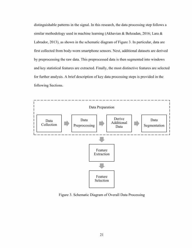
distinguishable patterns in the signal. In this research, the data processing step follows a
similar methodology used in machine learning (Akhavian & Behzadan, 2016; Lara &
Labrador, 2013), as shown in the schematic diagram of Figure 3. In particular, data are
first collected from body-worn smartphone sensors. Next, additional datasets are derived
by preprocessing the raw data. This preprocessed data is then segmented into windows
and key statistical features are extracted. Finally, the most distinctive features are selected
for further analysis. A brief description of key data processing steps is provided in the
following Sections.
Figure 3. Schematic Diagram of Overall Data Processing
Data Collection
Data
Preprocessing
Derive Additional
Data
Data
Segmentation
Data Preparation
Feature Extraction
Feature Selection

22
Data Preparation
In this Section, the steps for preparing sensor data (i.e. data collection, data
preprocessing, deriving additional data, and data segmentation) are discussed.
Data Collection. In the experiments conducted in this research, smartphones are
attached to different points of a person’s body (e.g. upper arm, waist), and readings from
the accelerometer, gyroscope, and linear acceleration sensors are recorded while that
person is carrying out different activities. An off-the-shelf application is launched on the
smartphone to log sensor readings at a sampling frequency of 180 Hz. The sampling
frequency is the reciprocal of the time between two consecutive measurements (Milette &
Stroud, 2012). The collected data is stored in comma-separated value (CSV) format in
each smartphone and then transferred to a personal computer. Next, values from the CSV
files are imported as numeric matrices in MATLAB and used in further computations.
Data Preprocessing. Theoretically, a sampling frequency of 180 Hz implies that
sensor readings will be recorded at every 1/180 seconds. However, in practice, a sensor
may fail to record flawless measurements at such a uniform time interval. The reason
behind this is that during the recording process, the sensor may occasionally freeze for a
short time and stop recording data. In this case, when the sensors recovers from freezing,
it tries to compensate for the missing values by recording data at a higher sampling
frequency (Akhavian, Brito, & Behzadan, 2015). Therefore, in order to obtain a
continuous and orderly data stream, collected data is processed into uniform time series
by removing the redundant data and linearly interpolating the missing values. A sample
MATLAB code for this process is given below:
% data is a M X N matrix of sensor readings
% 1st column of the data is timestamps
23
% Resampling timestamps
t_new = (data(1,1):(1/samplingRate):data(end,1))';
% Linear interpolation
TUdata = interp1(data(:,1),data(:,2:end),t_new,'linear');
Derive Additional Data. As previously described, sensors used in this research
return components of acceleration force, angular velocity, and linear acceleration along
three local Cartesian axes of the device. It was previously explained that more motion-
related data (namely the resultant acceleration force, three Cartesian components of jerk,
resultant jerk, resultant angular velocity, three Cartesian components of angular
acceleration, resultant angular acceleration, resultant linear acceleration force, three
Cartesian components of linear jerk, and resultant linear jerk) can be further derived
using Equations (1) through (4). A sample MATLAB code for deriving additional data
from accelerometer readings is given below.
% acc_data is M X 3 matrix which contains readings of tri-
axial accelerometer
resultant_acc = sqrt(acc_data(:,1).^2 + acc_data(:,2).^2 +
acc_data(:,3).^2);
jerk_data = diff(acc_data);
resultant_jerk = sqrt(jerk_data(:,1).^2 + jerk_data(:,2).^2 +
jerk_data(:,3).^2);
It should be noted that the requirement for deriving additional data from raw
sensor data depends on the application and the real value of such derived data in data
analysis. For instance, while some researchers (Anguita et al., 2013) derive additional
data from raw sensor readings to obtain more motion-related data, others (Akhavian &
Behzadan, 2016) have skipped this step and directly proceeded to data segmentation.

24
Data Segmentation. As expected, collecting raw data at a high sampling rate
results in significantly large datasets that are computationally inefficient to handle. To
address this issue, raw time series data need to be compressed by being segmented into
multiple windows. Moreover, while a single data point represents a momentary motion at
a single point of time, human activities (e.g. walking, running) consist of sequential
motions distributed over a period of time. Therefore, it is more logical to work with
windows of data points, rather than single data points, when dealing with human
activities. In this context, a window refers to a set of consecutive time series data points.
Mathematically, a time series of n data points, i.e. S = {S1, …, Sn}, can be represented as a
series of m windows, i.e., {W1, …, Wm}, where each Wi contains a series of k consecutive
data points, i.e. Wi = {Si1, …, Sik} (Lara & Labrador, 2013). In this case, the window size
refers to the number of data points in that window, and, often, presented as the duration
(i.e. difference between the timestamps of first and last data points) of that window in
seconds.
Data segmentation can be achieved with or without overlapping the adjacent
windows. Segmenting the data with overlapping windows is useful when there are
transitions between activities (Su, Tong, & Ji, 2014). Researchers have stated that
overlapping reduces the error resulted from transition state noise (Su et al., 2014).
Moreover, while window size can be fixed or variable, segmentation with fixed-sized
windows is computationally more efficient (Su et al., 2014). Considering these issues and
following the approach taken in past research (Akhavian & Behzadan, 2016), here, fixed-
sized windows with 50% overlap are selected for data segmentation.

25
Feature Extraction
After segmenting the time series data into windows, the next step is to extract a
set of key statistical features (a.k.a. feature vector) for each window which represents the
pattern of the signal in the corresponding window. For mathematical definition, consider
a window Wi of size k which contains m dimensions (i.e. sensor readings). This window
can be represented as a k by m matrix, as shown in Equation (5),
𝑊𝑖 = [
𝑆𝑖11 … 𝑆𝑖1𝑚… … …𝑆𝑖𝑘1 … 𝑆𝑖𝑘𝑚
] (5)
If n features are extracted for each dimension (i.e. column in the matrix
representation) of window Wi, the feature vector will have a total of m.n dimensions.
Mathematically, this feature vector can be defined by Equation (6),
𝐹𝑖 = {𝑓𝑖11, … , 𝑓𝑖1𝑛, … , 𝑓𝑖𝑚1, … 𝑓𝑖𝑚𝑛} (6)
in which, fixy = featurey(Si1x,…, Sikx). Here, featurey is a function that returns the yth
statistical feature for the sample Si1x, …, Sikx.
In general, features can be extracted in time and frequency domains. Time-
domain features are statistical measurements that represent the pattern of signal with
respect to time. Examples include mean, maximum, minimum, and standard deviation of
a sample data. On the other hand, frequency-domain features, such as energy and
entropy, represent data with respect to frequency and describe periodicity of the signal
(Lara & Labrador, 2013). Typically, frequency-domain features are extracted based on
fast Fourier transform (FFT) (Akhavian & Behzadan, 2016). Given the findings and
recommendations of past research in which time-domain features were used in data
mining for activity recognition using smartphones (Shoaib, Bosch, Incel, Scholten, &

26
Havinga, 2015), in this research, several time-domain features are extracted for data
analysis. The most commonly used time-domain features are briefly described in the
following paragraphs, and predefined functions in MATLAB for calculating those
features are listed in Table 2.
Table 2. Predefined Functions in MATLAB for Calculating Statistical Features.
Feature MATLAB Function
Mean mean
Maximum max
Minimum min
Standard deviation std
Mean absolute deviation mad
Interquartile range iqr
Skewness skewness
Kurtosis kurtosis
Autoregressive coefficients arburg
Mean. Mean is the simple arithmetic mean of a sample. Mathematically, the
mean of k data points can be calculated using Equation (7),
𝑀𝑒𝑎𝑛, 𝜇 = 1
𝑘∑𝑥𝑖
𝑘
𝑖=1
(7)
Maximum and Minimum. As the names imply, the maximum and minimum
refer to the maximum and minimum values in a sample, respectively.

27
Standard Deviation (SD). Standard deviation (𝜎) is the measure of variation,
dispersion, or spread in the data. Mathematically, it is the square root of the average
squared difference from the mean, as formulated in Equation (8),
𝑆𝐷, 𝜎 = √1
𝑘∑(𝑥𝑖 − 𝜇)
2
𝑘
𝑖=1
(8)
Mean Absolute Deviation (MAD). Mean absolute deviation is the arithmetic
mean of absolute difference from the mean, as mathematically shown in Equation (9),
𝑀𝐴𝐷 = 1
𝑘∑|𝑥𝑖 − 𝜇|
𝑘
𝑖=1
(9)
Interquartile Range (IQR). IQR is the difference between the 75th (3rd quartile,
or Q3) and the 25th percentiles (1st quartile, or Q1) of a sample, and is calculated using
Equation (10),
𝐼𝑄𝑅 = 𝑄3 − 𝑄1 (10)
Skewness. Skewness is the measure of asymmetry around the mean. A positive
skewness indicates that the data is spread out more to the right than to the left. A negative
skewness indicates the opposite scenario. For reference, the skewness of the Normal
distribution is always zero (since the distribution is perfectly symmetrical around the
mean). Mathematically, skewness can be calculated using Equation (11),
𝑆𝑘𝑒𝑤𝑛𝑒𝑠𝑠 =
1𝑘∑ (𝑥𝑖 − 𝜇)
3𝑘𝑖=1
(√1𝑘∑ (𝑥𝑖 − 𝜇)
2𝑘𝑖=1 )
3 (11)
Kurtosis. Kurtosis is the measure of how much a distribution of a sample is prone
to outliers. The kurtosis of the Normal distribution is equal to 3. A value higher than 3
28
means that the distribution is more prone to outliers. Mathematically, kurtosis can be
defined using Equation (12),
𝐾𝑢𝑟𝑡𝑜𝑠𝑖𝑠 =
1𝑘∑ (𝑥𝑖 − 𝜇)
4𝑘𝑖=1
(1𝑘∑ (𝑥𝑖 − 𝜇)
2𝑘𝑖=1 )
2 (12)
Autoregressive Coefficients. For a time-series stochastic process {Yt; t=0, 1, 2,
…}, an autoregressive model of pth order can be defined by Equation (13), in which 𝜑𝑖’s
(for i = 1, 2, …, p) are autoregressive coefficients, c is a constant, and 𝜀𝑡 is white noise,
i.e., independent (or uncorrelated) and identically distributed (zero mean) random
variables with constant variance (Cryer & Chen, 2008).
𝑌𝑡 = ∑𝜑𝑖𝑌𝑡−𝑖
𝑝
𝑖=1
+ 𝑐 + 𝜀𝑡 (13)
Feature Selection
Not all extracted features are useful since not all yield distinguishable (a.k.a.
distinctive) patterns. For example, it may turn out that a feature does not contain any
value-adding information and thus can be excluded from further computation. In order to
identify the most distinctive features, feature selection algorithms are applied to a dataset.
The goal of feature selection is thus to select the most relevant and useful features that
can be used to find any predefined patterns (a.k.a. class) in the signal. Two commonly
used feature selection algorithms are Correlation-based feature selection (CFS) and
ReliefF algorithms which are described in following paragraphs.
CFS Algorithm. The CFS algorithm uses a correlation-based approach and
heuristic search strategy to find a subset of the feature space. The subset contains features

29
that are highly correlated with the classes, yet uncorrelated to each other (Hall, 1999).
The main idea is to calculate the “merit” of a feature subset S, containing k features,
which is defined as shown in Equation (14),
𝑀𝑆 =
𝑘𝑟𝑐𝑓
√𝑘 + (𝑘 + 1)𝑟𝑓𝑓
(14)
where, 𝑟𝑐𝑓 is the average correlations between feature (f ϵ S) and class, and 𝑟𝑓𝑓 is
the average of feature to feature inter-correlations (Hall, 1999). The value of 𝑀𝑆 will be
higher if 𝑟𝑐𝑓 is higher, or in other words, if the features are highly correlated to classes.
Additionally, 𝑀𝑆 will be higher if 𝑟𝑓𝑓 is lower, or in other words, if the features are
uncorrelated to each other. The CFS algorithm performs a heuristic search to find all
possible subsets of the feature space, calculates the merit of each subset, and finally
returns the subset with the best merit.
ReliefF Algorithm. ReliefF is a feature selection algorithm that assigns weights
to the features and ranks them according to how well their values distinguish between
neighboring instances of same and different classes (Yu & Liu, 2003). This algorithm is
an extended version of Relief algorithm and works well on noisy, incomplete, and multi-
class dataset (Kononenko, 1994). According to Chikhi and Benhammada (2009), the
algorithm randomly selects an instance (i.e., a vector of feature values and the class
value) Ri, and searches for its k nearest neighbors from each of all possible classes. The
neighboring instances from the same class of Ri are called nearest hits and denoted as Hj,
where j=1, …, k. On the other hand, the neighboring instances from different classes are
called nearest misses. For class C, nearest misses are denoted as Mj(C), where j=1, …, k.
Depending on the values of Ri, Hj, and Mj(C), the algorithm updates the weights W(f) of

30
all the features f ϵ F. If the distance between Ri and Hj is high for feature f, it means that
the two neighboring instances of the same class are distant from each other (which is not
desirable). Therefore, the weight of the feature f, W(f), is subsequently reduced. On the
other hand, if the difference between Ri and Mj(C) is high for feature f, it means that two
neighboring instances of different classes are distant from each other (which is desirable).
Therefore, the weight of the feature f, W(f), is subsequently increased. The algorithm
updates the weights by combining the contributions of all the hits and misses, and iterates
the entire process for m times where m is defined by the user. MATLAB provides a
predefined function, i.e., relieff, for this algorithm which returns rankings and
weights of all features in a feature space. A sample code for applying the algorithm in
MATLAB is shown in below:
[ranks,weights] = relieff(feature_data,class_data,10);
Summary and Conclusions
Within the past decade, smartphones have emerged as ubiquitous computing
devices, and the incorporation of cutting edge mobile sensing technology has created
traction among researchers from various fields to explore its merit as a direct
measurement tool in ergonomic assessment. In general, modern smartphones are
equipped with a host of useful sensors which can be categorized into motion,
environmental, and position sensors. In particular, the on-board motion sensors (e.g.
accelerometer and gyroscope) of a smartphone allows for unobtrusively and
autonomously capturing of time-motion data which can be subsequently used in
identifying posture, recognizing activities, monitoring productivity, and evaluating
ergonomic risks associated with field activities.

31
The accelerometer sensor measures the acceleration force in terms of g-force, and
the gyroscope sensor measures the angular velocity in rad/s. Both sensors are hardware
sensors (i.e. physically located inside the device). MEMS accelerometer and gyroscope
sensors are made of electronic device some parts of which mechanically move when the
device is in motion. The parameters of this motion are extracted by measuring the
mechanical movement of those parts which are directly correlated to the changes in the
electronic capacity of the circuit inside the device. Unlike accelerometer and gyroscope,
the linear acceleration sensor is a software sensor which collects readings from the
accelerometer and outputs the acceleration force excluding the effect of gravitational
force.
In order to perform complex analysis such as HAR, smartphone’s raw signals
need to be transformed into useful features. To do this, first, the collected raw data from
smartphone sensors are processed into uniform time series data. Next, additional motion-
related data such as jerk and magnitude are derived. Processed data is then segmented
into a series of windows and key statistical features for each window are extracted.
Statistical features can be divided into two categories of time-domain and frequency-
domain features. In this research, time-domain statistical features (e.g. mean, maximum,
minimum, SD, MAD, IQR, skewness, kurtosis, and autoregressive coefficients) are
extracted and used. Finally, feature selection algorithms, such as ReliefF and CFS are
applied to select the most distinctive and useful subset of the extracted features.

32
ERGONOMIC ANALYSIS OF AWKWARD POSTURES
As mentioned in previous Chapters, awkward posture is one of the eight major
risk factors, identified by Occupational Safety and Health Administration (OSHA) that
causes or contributes to work-related musculoskeletal disorders (WMSDs). By definition,
an awkward posture is the posture in which one or more body parts are deviated from
their neutral positions (EU-OSHA, 2008). In contrast, a neutral posture is defined as a
posture in which muscles of different body parts are at close to their resting length, i.e.,
neither contracted nor elongated (University of Massachusetts Lowell, 2012). From this
perspective, any non-neutral posture can be essentially considered an awkward posture.
In a neutral posture, there are minimum stresses on the nerves, tendons, muscles and
bones, allowing for the utmost control of the body parts and exertion of maximum force
(Moore, Steiner, & Torma-Krajewski, 2011). In awkward postures, however, muscles
loss their capacity to produce force because of the deformation of muscle fibers and
friction with the bones (Clarke, 1966; Ozkaya N & Nordin M, 1999). For example, tying
rebar in stooping posture significantly reduces muscle activity in the lower-back region
(Umer, Li, Szeto, & Wong, 2017). Therefore, more muscular effort is needed to produce
the same amount of force as produced in neutral posture, resulting in muscular fatigue,
and increasing risk for WMSDs (Moore et al., 2011).
Risk Assessment of Awkward Postures
For the assessment of risks associated with awkward postures, generally, postures
of different body parts (e.g. trunk, shoulder, neck, knee, elbow) are measured in terms of
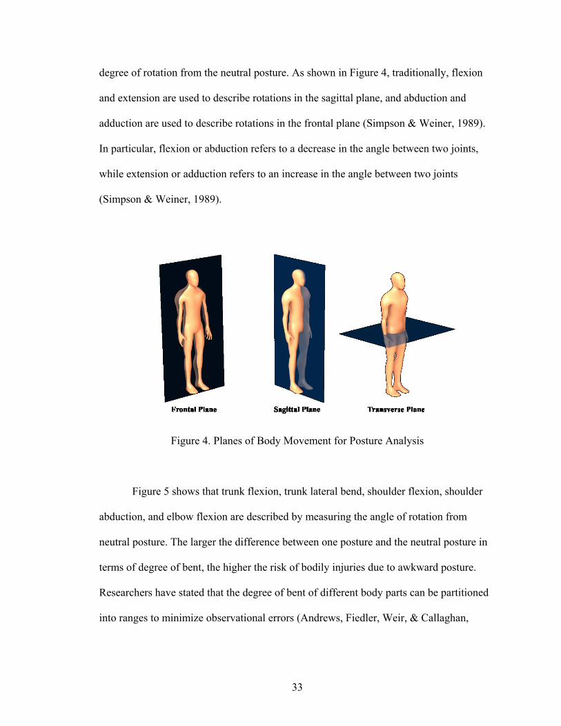
33
degree of rotation from the neutral posture. As shown in Figure 4, traditionally, flexion
and extension are used to describe rotations in the sagittal plane, and abduction and
adduction are used to describe rotations in the frontal plane (Simpson & Weiner, 1989).
In particular, flexion or abduction refers to a decrease in the angle between two joints,
while extension or adduction refers to an increase in the angle between two joints
(Simpson & Weiner, 1989).
Figure 4. Planes of Body Movement for Posture Analysis
Figure 5 shows that trunk flexion, trunk lateral bend, shoulder flexion, shoulder
abduction, and elbow flexion are described by measuring the angle of rotation from
neutral posture. The larger the difference between one posture and the neutral posture in
terms of degree of bent, the higher the risk of bodily injuries due to awkward posture.
Researchers have stated that the degree of bent of different body parts can be partitioned
into ranges to minimize observational errors (Andrews, Fiedler, Weir, & Callaghan,
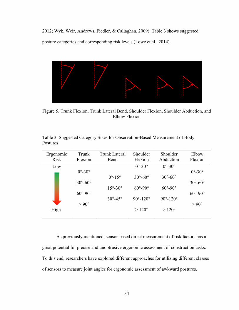
34
2012; Wyk, Weir, Andrews, Fiedler, & Callaghan, 2009). Table 3 shows suggested
posture categories and corresponding risk levels (Lowe et al., 2014).
Figure 5. Trunk Flexion, Trunk Lateral Bend, Shoulder Flexion, Shoulder Abduction, and
Elbow Flexion
Table 3. Suggested Category Sizes for Observation-Based Measurement of Body
Postures
Ergonomic
Risk
Trunk
Flexion
Trunk Lateral
Bend
Shoulder
Flexion
Shoulder
Abduction
Elbow
Flexion
Low
High
0°-30°
30°-60°
60°-90°
> 90°
0°-15°
15°-30°
30°-45°
0°-30°
30°-60°
60°-90°
90°-120°
> 120°
0°-30°
30°-60°
60°-90°
90°-120°
> 120°
0°-30°
30°-60°
60°-90°
> 90°
As previously mentioned, sensor-based direct measurement of risk factors has a
great potential for precise and unobtrusive ergonomic assessment of construction tasks.
To this end, researchers have explored different approaches for utilizing different classes
of sensors to measure joint angles for ergonomic assessment of awkward postures.

35
Examples include using magneto-resistive angle sensors to measure shoulder flexion
(Alwasel et al., 2011), and Kinect or depth sensors to analyze posture by detecting
position of skeleton joints at high sampling rates (Diego-Mas & Alcaide-Marzal, 2014;
Más et al., 2014; Plantard et al., 2015). In particular, IMU sensors have been widely used
for tensor decomposition and posture classification (Chen, Qiu, & Ahn, 2017), posture
assessment (Yan, Li, Li, & Zhang, 2017), capturing spinal kinematics (Umer et al.,
2017), and for measuring knee flexion or extension angles (Seel, Raisch, & Schauer,
2014), multiple joint angles (Vignais et al., 2013), and gait stability (Jebelli, Ahn, &
Stentz, 2014).
However, almost all such studies required the tedious process of setting up,
synchronizing, calibrating, and using a sophisticated sensor network, which often
requires expertise that is normally beyond what is expected from construction personnel
and practitioners. Even if such skills are available, the upfront investment to purchase,
install, and maintain the equipment, as well as the necessary time commitment may
hinder the success of the effort (David, 2005). To overcome these implementation
challenges, in the discussions and experiments presented in this Chapter, smartphones are
used as data collection devices due to their ubiquity, low procurement and maintenance
cost, and ease of use. Moreover, a novel scientific methodology is introduced to
autonomously calculate the ergonomic risk levels from features extracted from
smartphone sensor data. The data collection and feature extraction methodology was
described in detail in previous Chapter. The main focus of this Chapter is on the
implementation of the developed methodology in a series of field experiments. In the
following Sections, the proposed hypothesis and several corollary propositions are first
36
described. Next, an equation is derived to calculate joint angles in more practical terms.
Finally, a detailed discussion of the field experiments carried out to test the hypothesis
and evaluate the practicality of using smartphones for ergonomics assessment of
construction tasks is presented.
Hypothesis
For ergonomic analysis, generally, body postures are determined by measuring
angular rotations of different body parts, e.g. trunk flexion, trunk lateral bend, shoulder
flexion, shoulder abduction, elbow flexion, neck bent, neck twist, wrist bent, forearm
twist, knee angle, and ankle posture (Lowe et al., 2014; University of Massachusetts
Lowell, 2012). In this research, a body posture is defined as a vector that consists of
angular rotations of m different body parts, as shown in Equation (15),
𝑇𝑖 = [
𝛽𝑖1𝛽𝑖2…𝛽𝑖𝑚
] (15)
where 𝛽𝑖𝑚 is the angular rotation of body part m in posture vector 𝑇𝑖. For example, a
posture vector 𝑇1, consisting of five components, namely trunk flexion (TF), trunk lateral
bend (TLB), shoulder flexion (SF), shoulder abduction (SA), and elbow flexion (EF), can
be expressed by Equation (16),
𝑇1 =
[ 𝑇𝐹1𝑇𝐿𝐵1𝑆𝐹1𝑆𝐴1𝐸𝐹1 ]
(16)
Using the definition presented in Equation (15), the neutral posture (T0) is a null
(i.e. zero) vector and can be expressed by Equation (17),

37
𝑇0 = [
00…0
] (17)
As a convention, a feature 𝑓𝑒𝑎𝑡𝑢𝑟𝑒𝑘 corresponding to a posture 𝑇𝑖 is denoted as
𝑇𝑖 . 𝑓𝑒𝑎𝑡𝑢𝑟𝑒𝑘. A feature is normalized by subtracting the corresponding feature obtained
from the neutral posture from it. Normalized features are denoted as 𝑇𝑖 . 𝑓𝑒𝑎𝑡𝑢𝑟𝑒𝑘′ and
mathematically expressed by Equation (18),
𝑇𝑖 . 𝑓𝑒𝑎𝑡𝑢𝑟𝑒𝑘′ = 𝑇𝑖 . 𝑓𝑒𝑎𝑡𝑢𝑟𝑒𝑘 − 𝑇0. 𝑓𝑒𝑎𝑡𝑢𝑟𝑒𝑘 (18)
It is thus imperative that the normalized feature vector for the neutral posture also
be a null vector.
Using this convention, if a posture S can be expressed as the weighted sum of n
base postures (T1, T2, T3, …, Tn), as shown in Equation (19) (referred to as posture
composition equation) then it is hypothesized that a normalized features 𝑓𝑒𝑎𝑡𝑢𝑟𝑒𝑘
extracted from sensory data while the worker is in posture S can be expressed as the
weighted sum of that same normalized feature 𝑓𝑒𝑎𝑡𝑢𝑟𝑒𝑘 extracted from sensory data
corresponding to base postures (T1, T2, T3, …, Tn), as shown in Equation (20) (referred to
as feature composition equation). Additionally, the weight of 𝑓𝑒𝑎𝑡𝑢𝑟𝑒𝑘 for each base
posture, 𝑓𝑘(𝛼𝑖) in the feature composition equation, is a function of the corresponding
weight of the same base postures, αi in the posture composition equation. This can be
mathematically formulated by Equation (19) and Equation (20); that is, if,
𝑆 = 𝛼1𝑇1 + 𝛼2𝑇2 +⋯+ 𝛼𝑛𝑇𝑛 =∑ 𝛼𝑖𝑇𝑖
𝑛
𝑖=1 (19)
then,

38
𝑆. 𝑓𝑒𝑎𝑡𝑢𝑟𝑒𝑘′ = 𝑓𝑘(𝛼1)𝑇1. 𝑓𝑒𝑎𝑡𝑢𝑟𝑒𝑘′ + 𝑓𝑘(𝛼2)𝑇2. 𝑓𝑒𝑎𝑡𝑢𝑟𝑒𝑘′ + ⋯
+ 𝑓𝑘(𝛼𝑛)𝑇𝑛. 𝑓𝑒𝑎𝑡𝑢𝑟𝑒𝑘′ = ∑ 𝑓𝑘(𝛼𝑖)𝑇𝑖 . 𝑓𝑒𝑎𝑡𝑢𝑟𝑒𝑘′𝑛
𝑖=1
(20)
Mathematical Analysis of the Hypothesis
In this section, several corollary propositions are developed, based on the
hypothesis described in previous section, which are further used to discover the
relationship between the posture vector and the extracted features.
Posture Composition Weight Factors, α. Assume a general posture vector Ti
consisting of m number of components (denoted with β) which is mathematically
expressed by Equation (15). Then, from Equation (19), any given posture S can be
written as,
𝑆 = 𝛼1𝑇1 + 𝛼2𝑇2 +⋯+ 𝛼𝑛𝑇𝑛
= 𝛼1
[ ᵝ11ᵝ12ᵝ13…ᵝ1𝑚]
+ 𝛼2
[ ᵝ21ᵝ22ᵝ23…ᵝ2𝑚]
+ ⋯+ 𝛼𝑛
[ ᵝ𝑛1ᵝ𝑛2ᵝ𝑛3…ᵝ𝑛𝑚]
(21)
According to Equation (21), posture S can be expressed as the weighted sum of n
base postures T, using n unknown multipliers (α1, α2, α3, …, αn) and m independent
equations. If n = m, then the number of unknowns will be equal to the number of
independent equations, and hence, Equation (21) can be mathematically solved.
Substituting n for m in Equation (21), a given posture S can be written as shown in
Equation (22),

39
𝑆 =
[ α1α2α3…α𝑚]
[ ᵝ11 ᵝ21 ᵝ31 … ᵝ𝑚1ᵝ12 ᵝ22 ᵝ32 … ᵝ𝑚2ᵝ13…ᵝ1𝑚
ᵝ23…ᵝ2𝑚
ᵝ33…ᵝ3𝑚
………
ᵝ𝑚3…ᵝ𝑚𝑚]
(22)
Alternately, Equation (22) can be rewritten in matrix form, as shown in Equation
(23), and posture composition weight factors (α) can be calculated by matrix operations.
𝑆 = 𝛼. 𝑇 𝑠𝑜𝑙𝑣𝑖𝑛𝑔 𝑓𝑜𝑟 𝛼⇒ 𝛼 = 𝑇−1. 𝑆 (23)
Feature Composition Weight Factors, f(α). Assume that an arbitrary posture S
is identical to any given base posture 𝑇𝑖. Therefore, Equation (19) can be rewritten as
shown in Equation (24).
𝑇𝑖 = 𝛼1𝑇1 +⋯+ 𝛼𝑖𝑇𝑖 +⋯+ 𝛼𝑛𝑇𝑛 (24)
Equating coefficient of 𝑇𝑖’s in both sides of the Equation (24), 𝛼𝑖 = 1, and 𝛼𝑗 = 0
for all j ≠ i. In this case, features of posture S are identical to features of base posture 𝑇𝑖,
i.e., 𝑆. 𝑓𝑒𝑎𝑡𝑢𝑟𝑒𝑘′ = 𝑇𝑖 . 𝑓𝑒𝑎𝑡𝑢𝑟𝑒𝑘′ for all k, and thus, Equation (20) can be rewritten as
shown in Equation (25).
𝑇𝑖 . 𝑓𝑒𝑎𝑡𝑢𝑟𝑒𝑘′ = 𝑓𝑘(𝛼1)𝑇1. 𝑓𝑒𝑎𝑡𝑢𝑟𝑒𝑘′ + …+ 𝑓𝑘(𝛼𝑖)𝑇𝑖 . 𝑓𝑒𝑎𝑡𝑢𝑟𝑒𝑘′
+ ⋯+ 𝑓𝑘(𝛼𝑛)𝑇𝑛. 𝑓𝑒𝑎𝑡𝑢𝑟𝑒𝑘′ (25)
Similarly, equating coefficient of 𝑇𝑖 . 𝑓𝑒𝑎𝑡𝑢𝑟𝑒𝑘′’s in both sides of the Equation
(25) yields 𝑓𝑘(𝛼𝑖) = 1, and 𝑓𝑘(𝛼𝑗) = 0 for all j ≠ i. This important observation serves as
the basis for establishing key boundary conditions when attempting to find a
mathematical relationship between α values and corresponding f(α) values. In summary,
the boundary conditions can be expressed as shown in Equation (26),
𝛼𝑖 = 0 𝑡ℎ𝑒𝑛→ 𝑓𝑘(𝛼𝑖) = 0 , and 𝛼𝑖 = 1
𝑡ℎ𝑒𝑛→ 𝑓𝑘(𝛼𝑖) = 1 , for all k (26)

40
From the two boundary conditions introduced in Equation (26), it can be inferred
that the mathematical function f(α) can be linear, polynomial, or trigonometric. Example
of these functions are shown in Table 4.
Table 4. Sample Mathematical Functions Relating Posture Composition and Feature
Composition Weight Factors
Function Type Example
Linear f(α)= α
Polynomial f(α)= αm
Trigonometric f(α)= sin(90α)
Feature Normalization. As stated earlier, in Equation (20) all features are
normalized. In order to understand why normalization is necessary, first assume that the
features are not normalized and denoted as 𝑇𝑖 . 𝑓𝑒𝑎𝑡𝑢𝑟𝑒𝑘. Then, Equation (20) can be
rewritten as shown in Equation (27),
𝑆. 𝑓𝑒𝑎𝑡𝑢𝑟𝑒𝑘 =∑ 𝑓𝑘(𝛼𝑖)𝑇𝑖 . 𝑓𝑒𝑎𝑡𝑢𝑟𝑒𝑘
𝑛
𝑖=1 (27)
For, S = T0 (with T0 denoting the neutral posture) 𝛼𝑖 = 0 for all i, hence, from
Equation (26), 𝑓𝑘(𝛼𝑖) = 0 for all i. Therefore, Equation (27) can be written as Equation
(28),
𝑇0. 𝑓𝑒𝑎𝑡𝑢𝑟𝑒𝑘 = 0 (28)
However, features of neutral posture may not be necessarily zero (e.g.
accelerometer’s Y-axis reads the value of 1 in neutral posture, if the device’s Y-axis is

41
oriented vertically downward). Therefore, in order for Equation (27) to be consistent with
the boundary conditions, an arbitrary constant, C, is added, as shown in Equation (29),
𝑆. 𝑓𝑒𝑎𝑡𝑢𝑟𝑒𝑘 =∑ 𝑓𝑘(𝛼𝑖)𝑇𝑖 . 𝑓𝑒𝑎𝑡𝑢𝑟𝑒𝑘
𝑛
𝑖=1+ 𝐶 (29)
Next, applying the first boundary condition (i.e. for S = T0, 𝛼𝑖 = 0 and hence
𝑓𝑘(𝛼𝑖) = 0) to Equation (29) yields 𝐶 = 𝑇0. 𝑓𝑒𝑎𝑡𝑢𝑟𝑒𝑘. Therefore, Equation (29) can be
rewritten as Equation (30),
𝑆. 𝑓𝑒𝑎𝑡𝑢𝑟𝑒𝑘 − 𝑇0. 𝑓𝑒𝑎𝑡𝑢𝑟𝑒𝑘 =∑ 𝑓𝑘(𝛼𝑖)𝑇𝑖 . 𝑓𝑒𝑎𝑡𝑢𝑟𝑒𝑘
𝑛
𝑖=1
⇒ 𝑆. 𝑓𝑒𝑎𝑡𝑢𝑟𝑒𝑘′ = ∑ 𝑓𝑘(𝛼𝑖)𝑇𝑖. 𝑓𝑒𝑎𝑡𝑢𝑟𝑒𝑘𝑛
𝑖=1
(30)
Applying the second boundary condition to Equation (30) (i.e. for S = Ti, 𝛼𝑖 = 1
and 𝛼𝑗 = 0 for all j ≠ i, hence 𝑓𝑘(𝛼𝑖) = 1 and 𝑓𝑘(𝛼𝑖) = 0 for all j ≠ i), yields,
𝑇𝑖 . 𝑓𝑒𝑎𝑡𝑢𝑟𝑒𝑘′ = 𝑇𝑖 . 𝑓𝑒𝑎𝑡𝑢𝑟𝑒𝑘 (31)
Equation (30) and Equation (31) show that all features, either of combined posture
(S) or of any base posture (Ti), should be normalized to satisfy both boundary conditions.
Mathematical Analysis of Constraints
In previous Section, general corollary propositions are developed based on the
stated hypothesis. In this Section, a more specific mathematical analysis is performed for
static postures. First, several constraints are identified considering the physics of static
postures and limitations of smartphone sensors. Next, mathematical analyses are
performed based on the selected constraints.
Identification of Constraints. As mentioned earlier, smartphone’s accelerometer
sensor returns three components of acceleration force. However, a stationary

42
accelerometer (i.e. in the absence of any physical acceleration) provides value-adding
information about two axes only, with the third derivable from the other two, as shown in
the example of Equation (32),
𝑎𝑧 = √1 − 𝑎𝑥
2 − 𝑎𝑦2 (32)
This Equation is true since for a static (not moving) sensor, the resultant
acceleration force is always 1g. In other words, accelerometer can measure two degrees
of freedom in a static condition. Moreover, for a static posture, gyroscope and linear
acceleration sensors do not provide any value-adding information because the angular
velocity and body acceleration associated with static activities are very negligible
(theoretically, zero). Therefore, using only the motion sensors (i.e. accelerometer,
gyroscope, and linear acceleration sensor) of a smartphone, it is not possible to measure a
posture vector that consists of more than two components (i.e. two degrees of freedom).
In this Thesis, and within the scope of this research, it is assumed that posture vectors
consist of only one component, i.e., rotations of a body part are confined to one plane (or
along one axis).
Now, assume that a smartphone is attached to a body part. As shown in Figure
6(a), for neutral posture, the smartphone’s Y-axis is oriented vertically downward. When
the body part rotates β° anti-clockwise about the Z-axis of the smartphone, its orientation
is changed as shown in Figure 6(b). Since the gravitational force acts downward along
the vertical axis, its components along X and Y axes, measured by the accelerometer, can
be expressed using Equations (33) and (34), in which 𝑎𝑥 and 𝑎𝑦 represent raw signals
from the accelerometer.

43
𝑎𝑥 = −sin(𝛽) (33)
𝑎𝑦 = cos(𝛽) (34)
Figure 6. Orientation of Smartphone While Rotating Along Z-axis
To correlate the pattern of raw signals with the extracted features from
accelerometer, a preliminary test is performed as follows: pointing the smartphone’s local
Y-axis vertically downward, the device is slowly rotated for 360° along its Z-axis (as
shown in Figure 6) at a near-uniform rate. Sensor readings, shown in Figure 7, reveal that
Accelerometer-X readings follow a sine curve while Accelerometer-Y readings follow a
cosine curve as theoretically shown in Equations (33) and (34). However, while
Accelerometer-Z readings must be theoretically zero, the abrupt peaks found in the
readings are resulted from handling error caused due to manually performing the rotation.
A closer look at the Accelerometer-X signal, as shown in Figure 8, reveals that
although patterns of upper and lower envelopes (i.e. outline of the extremes in high-
frequency data), and average of the signal are similar to the patterns observed in the raw
data (i.e. sine curve), there is a slight offset.
Y
X
Y
X
1
g
1g β
(a) Neutral
posture
(b) Rotating β° anti-clockwise
along Z-axis

44
Figure 7. Accelerometer Readings for 360-degree Rotation of a Smartphone
Figure 8. Low, Mean, and High Envelopes of Accelerometer-X Readings
Since upper, lower, and average envelope represent the maximum, minimum, and
mean of data features, respectively, for a given window, it can be inferred that for these
specific features, extracted from Accelerometer-X sensor, 𝑓𝑘(𝛼) would also be a sine
function of angular rotation (𝛽) of a body part. For convention, from this point forward,
the subscript k is substituted with X and Y to show that features are extracted from
Accelerometer-X and -Y, respectively. Following this convention, 𝑓𝑋(𝛼) can be written
in the general form of a sine function, as shown in Equation (35),
-1.5
-1
-0.5
0
0.5
1
1.5
-2 0 2 4 6 8 10 12 14 16 18
Acc
eler
om
eter
rea
din
g (
g)
Time (Sec)
X Y Z
-1.5
-1
-0.5
0
0.5
1
1.5
0 2 4 6 8 10 12 14 16 18
Acc
eler
om
eter
rea
din
g (
g)
Time (Sec)
Upper Env Average Lower Env

45
𝑓𝑋(𝛼) = 𝑎 sin(𝛽) + 𝑐 (35)
Similarly, for Accelerometer-Y, 𝑓𝑌(𝛼) would be a cosine function and the general
form can be expressed as shown in Equation (36),
𝑓𝑌(𝛼) = 𝑎 cos(𝛽) + 𝑐 (36)
It should be noted that Equations (35) and (36) may not be true for other features,
e.g., SD, MAD, IQR. Therefore, for further mathematical analysis, the feature space is
limited to the mean, minimum, and maximum of Accelerometer-X and -Y data only, as
shown in Equation (37),
𝐹𝑒𝑎𝑡𝑢𝑟𝑒 𝑠𝑝𝑎𝑐𝑒, 𝐹 = {
𝐴𝑐𝑐𝑒𝑙𝑒𝑟𝑜𝑚𝑒𝑡𝑒𝑟_𝑋_𝐴𝑣𝑔, 𝐴𝑐𝑐𝑒𝑙𝑒𝑟𝑜𝑚𝑒𝑡𝑒𝑟_𝑌_𝐴𝑣𝑔,𝐴𝑐𝑐𝑒𝑙𝑒𝑟𝑜𝑚𝑒𝑡𝑒𝑟_𝑋_𝑀𝑖𝑛, 𝐴𝑐𝑐𝑒𝑙𝑒𝑟𝑜𝑚𝑒𝑡𝑒𝑟_𝑌_𝑀𝑖𝑛,𝐴𝑐𝑐𝑒𝑙𝑒𝑟𝑜𝑚𝑒𝑡𝑒𝑟_𝑋_𝑀𝑎𝑥, 𝐴𝑐𝑐𝑒𝑙𝑒𝑟𝑜𝑚𝑒𝑡𝑒𝑟_𝑌_𝑀𝑎𝑥
} (37)
To summarize the discussion, the constraints are as follows:
1. A posture vector consists of one component, i.e., 𝛽.
2. The feature space F is defined by Equation (37).
3. The orientation of the smartphone is such that for neutral posture, its Y-axis is
pointing vertically downward and its rotation is confined to the XY plane.
Based on the aforementioned constraints, feature composition weight factors, f(α),
is found to be trigonometric function as shown in Equation (36) and (37).
Derivation of Formula for Measuring Posture Component. Based on the first
constraint, assume that each posture vector consists of a single component, i.e., 𝛽𝑖 for
posture Ti. As previously discussed, the number of base postures should be selected as
equal to the number of components of a posture vector. Therefore, in this case, one base
posture T, consisting of one component 𝛽𝑇, is selected. From Equation (19), a posture
vector S that consists of one component 𝛽𝑆 can be written as shown in Equation (38),

46
𝑆 = 𝛼𝑇 ⇒ 𝛽𝑆 = 𝛼𝛽𝑇 (38)
From Equation (20), a normalized feature 𝑓𝑒𝑎𝑡𝑢𝑟𝑒𝑘′ of posture S can be
expressed by Equation (39),
𝑆. 𝑓𝑒𝑎𝑡𝑢𝑟𝑒𝑘′ = 𝑓𝑘(𝛼)𝑇. 𝑓𝑒𝑎𝑡𝑢𝑟𝑒𝑘′ (39)
As shown in Equation (35), for all 𝑓𝑒𝑎𝑡𝑢𝑟𝑒𝑘 𝜖 𝐹 extracted from Accelerometer-
X, 𝑓𝑋(𝛼) can be written as in Equation (40),
𝑓𝑋(𝛼) = 𝑎 sin(𝛽𝑆) + 𝑐 = 𝑎 sin(𝛼𝛽𝑇) + 𝑐 (40)
From the first boundary condition, it is known that for α = 0, f(α) = 0. Hence,
from Equation (40), c = 0. From the second boundary condition, which is, for α = 1, f(α)
= 1, using Equation (40) and knowing that c = 0, it is concluded that 𝑎 = 1 sin (𝛼𝛽𝑇)⁄ .
Substituting the values of a and c in Equation (40),
𝑓𝑋(𝛼) =
sin(𝛽𝑆)
sin(𝛽𝑇) (41)
Therefore, for Accelerometer-X, substituting the value of 𝑓𝑋(𝛼) in Equation (39) yields,
𝑆. 𝑓𝑒𝑎𝑡𝑢𝑟𝑒𝑋
′ = sin(𝛽𝑆)
sin(𝛽𝑇)𝑇. 𝑓𝑒𝑎𝑡𝑢𝑟𝑒𝑋
′ (42)
Solving for 𝛽𝑆,
𝛽𝑆 = 𝑠𝑖𝑛−1 [sin(𝛽𝑇)
𝑆. 𝑓𝑒𝑎𝑡𝑢𝑟𝑒𝑋′
𝑇. 𝑓𝑒𝑎𝑡𝑢𝑟𝑒𝑋′ ] (43)
Similarly, from Equation (35), for all 𝑓𝑒𝑎𝑡𝑢𝑟𝑒𝑘 𝜖 𝐹 extracted from
Accelerometer-Y, 𝑓𝑌(𝛼) can be written as in Equation (44),
𝑓𝑌(𝛼) = 𝑎 cos(𝛽𝑆) + 𝑐 = 𝑎 cos(𝛼𝛽𝑇) + 𝑐 (44)
From the first boundary condition, i.e., for α = 0, f(α) = 0, using Equation (44) it is
deduced that a + c = 0. From the second boundary condition, which is, for α = 1, f(α) = 1,

47
using Equation (44) and knowing that a + c = 0, it is concluded that 𝑎 = 1
cos(𝛽𝑇)−1 and
𝑐 = −1
cos(𝛽𝑇)−1. Substituting the values of a and c in Equation (44),
𝑓𝑌(𝛼) =
cos(𝛽𝑆) − 1
cos(𝛽𝑇) − 1 (45)
For Accelerometer-Y, substituting the value of 𝑓𝑌(𝛼) in Equation (39) yields,
𝑆. 𝑓𝑒𝑎𝑡𝑢𝑟𝑒𝑌
′ = cos(𝛽𝑆) − 1
cos(𝛽𝑇) − 1𝑇. 𝑓𝑒𝑎𝑡𝑢𝑟𝑒𝑌
′ (46)
Solving for 𝛽𝑆,
𝛽𝑆 = 𝑐𝑜𝑠−1 [1 −
𝑆. 𝑓𝑒𝑎𝑡𝑢𝑟𝑒𝑌′
𝑇. 𝑓𝑒𝑎𝑡𝑢𝑟𝑒𝑌′ + cos(𝛽𝑇)
𝑆. 𝑓𝑒𝑎𝑡𝑢𝑟𝑒𝑌′
𝑇. 𝑓𝑒𝑎𝑡𝑢𝑟𝑒𝑌′ ] (47)
Equation (43) and (47)can be combined and expressed in the form of Equation
(48).
𝛽𝑆 =
{
𝑠𝑖𝑛−1 [sin(𝛽𝑇)
𝑆. 𝑓𝑒𝑎𝑡𝑢𝑟𝑒𝑋′
𝑇. 𝑓𝑒𝑎𝑡𝑢𝑟𝑒𝑋′ ] , 𝑓𝑜𝑟 𝐴𝑐𝑐_𝑋
𝑐𝑜𝑠−1 [1 −𝑆. 𝑓𝑒𝑎𝑡𝑢𝑟𝑒𝑌
′
𝑇. 𝑓𝑒𝑎𝑡𝑢𝑟𝑒𝑌′ + cos(𝛽𝑇)
𝑆. 𝑓𝑒𝑎𝑡𝑢𝑟𝑒𝑌′
𝑇. 𝑓𝑒𝑎𝑡𝑢𝑟𝑒𝑌′ ] , 𝑓𝑜𝑟 𝐴𝑐𝑐_𝑌
(48)
Equation (48) can be interpreted as follows: if a base posture T’s component 𝛽𝑇
and a normalized feature 𝑇. 𝑓𝑒𝑎𝑡𝑢𝑟𝑒𝐾′ are known, for any arbitrary posture S, its
component 𝛽𝑆 can be calculated from the extracted normalized feature of that posture
(i.e., 𝑆. 𝑓𝑒𝑎𝑡𝑢𝑟𝑒𝐾′ ). In other words, for any arbitrary posture, angular rotation of a body
part can be calculated from a feature extracted from the accelerometer sensor of a
smartphone attached to that part of the body. The premise is features are calibrated for a
neutral posture and a known base posture.
Consideration for Dynamic Activities. It should be noted that Equation (48)
consists of inverse trigonometric functions and as such, the arguments of each function

48
must be within the range of ±1. However, this may not be always the case. For instance, a
body part may experience accelerations in such a way that the component acceleration in
X- or Y-axis is more than 1g. But, since the discussions and mathematical analyses
performed so far are intended for static body postures, it is safe to assume that there is no
significant body acceleration present in the activities. However, in the presence of such
acceleration, one possible remedy would be to exclude the body acceleration from raw
accelerometer’s readings before employing Equation (48). As mentioned earlier, body
acceleration is measured by the linear acceleration sensor. Therefore, linear
accelerometer’s readings should be subtracted from the accelerometer’s readings to
exclude the effect of body acceleration, i.e., considering only the gravitational
acceleration. By doing so, the application of Equation (48) is broadened and no longer
limited to static activities. In other words, regardless of the presence of acceleration in the
body part (e.g. when a person is performing a dynamic activity), Equation (48) will yield
valid results for the orientation of the body part if only the gravitational acceleration is
considered. However, in this Chapter, the validity of Equation (48) is examined for static
activities only.
Validation Experiment
To verify the validity of the proposed hypothesis, the task of manual screw
driving is selected for posture analysis of a static activity. In the conducted experiments,
two smartphones are mounted on a worker’s body, one on the upper-arm and another on
the waist. As shown in Figure 9, data is collected from both smartphones for sixteen
different body postures. In this experiment, total flexion is defined as combined flexions

49
of trunk and shoulder (TF and SF). For the specific task of screw driving, as shown in the
postures of Figure 9, TF involves downward angular movements while SF involves
upward angular movements. Therefore, the total flexion is measured by subtracting TF
from SF, as formulated in Equation (49),
𝑇𝑜𝑡𝑎𝑙 𝐹𝑙𝑒𝑥𝑖𝑜𝑛 = 𝑆ℎ𝑜𝑢𝑙𝑑𝑒𝑟 𝐹𝑙𝑒𝑥𝑖𝑜𝑛 (𝑆𝐹) − 𝑇𝑟𝑢𝑛𝑘 𝐹𝑙𝑒𝑥𝑖𝑜𝑛 (𝑇𝐹) (49)
Figure 9. Sixteen Postures for the Screw Driving Experiment

50
To determine ground truth (a.k.a. observed) values, flexions are measured from
the photographs taken during the experiment. Referring to the sixteen postures shown in
Figure 9, observed values of trunk, shoulder, and total flexions are tabulated in Table 5.
Table 5. Observed Values of Trunk, Shoulder, and Total Flexion for the Sixteen Postures
Posture TF (°) SF (°) Total Flexion (°)
P1 0 0 0
P2 0 90 90
P3 0 120 120
P4 0 30 30
P5 30 60 30
P6 90 90 0
P7 0 45 45
P8 40 40 0
P9 30 85 55
P10 35 130 95
P11 40 40 0
P12 40 100 60
P13 45 125 80
P14 25 115 90
P15 25 90 65
P16 90 160 70

51
Data Analysis
As mentioned earlier, in this research it is assumed that a smartphone will
measure one component of a posture vector. Therefore, data collected from the
smartphone on the upper arm is used for measuring total flexion, while data collected
from the smartphone on the waist is used to measure TF. Finally, by combining the
results from the two smartphones, TF and SF values are determined. The values
calculated from the sensory data are referred to extracted values.
Equation for Measuring Flexions. Since all angles are zero for posture P1
(Table 5), this posture is considered as the neutral posture. As previously discussed, the
number of base postures should be selected as equal to the number of components of a
posture vector. In this experiment, each posture vector consists of a single component,
which is the total flexion for the upper arm-mounted smartphone and the TF for the
waist-mounted smartphone. Therefore, one base posture must be selected for analysis in
each case. Here, as a base posture T, posture P2 is selected for the upper arm-mounted
smartphone, and posture P6 is selected for the waist-mounted smartphone. In both cases,
the posture component (𝛽𝑇) is 90°. Therefore, by substituting 𝛽𝑇 = 90° in Equation (48),
Equation (50) is derived for calculating posture component 𝛽𝑆 for posture S.
𝛽𝑆 =
{
𝑠𝑖𝑛−1 [
𝑆. 𝑓𝑒𝑎𝑡𝑢𝑟𝑒𝑋′
𝑇. 𝑓𝑒𝑎𝑡𝑢𝑟𝑒𝑋′ ] , 𝑓𝑜𝑟 𝐴𝑐𝑐_𝑋
𝑐𝑜𝑠−1 [1 −𝑆. 𝑓𝑒𝑎𝑡𝑢𝑟𝑒𝑌
′
𝑇. 𝑓𝑒𝑎𝑡𝑢𝑟𝑒𝑌′ ] , 𝑓𝑜𝑟 𝐴𝑐𝑐_𝑌
(50)
Here, for the upper-arm mounter smartphone, 𝛽𝑆 refers to total flexion for posture
S and base posture T = P2, while for the waist-arm mounter smartphone, 𝛽𝑆 refers to TF
for posture S and base posture T = P6.

52
Comparison of Features. It can be seen that using Equation (50), 𝛽𝑆 can be
calculated in six different ways by using the six features in feature space F, as described
in Equation (37). To compare the effectiveness of these features, the first six postures (i.e.
P1 to P6) are selected for testing. Substituting 𝛽𝑇 = 90° in Equations (42) and (46), and
combining these two Equations, Equation (51) is derived, as follows,
𝑆. 𝑓𝑒𝑎𝑡𝑢𝑟𝑒𝑘
′ = {sin(𝛽𝑆) 𝑇. 𝑓𝑒𝑎𝑡𝑢𝑟𝑒𝑋
′ , 𝑓𝑜𝑟 𝐴𝑐𝑐_𝑋
1 − cos(𝛽𝑆) 𝑇. 𝑓𝑒𝑎𝑡𝑢𝑟𝑒𝑌′ , 𝑓𝑜𝑟 𝐴𝑐𝑐_𝑌
(51)
Knowing 𝛽 for the six selected postures (from Table 5) and given the extracted
features for the neutral (P1) and base postures (P2 for upper-arm mounted smartphone,
and P2 for waist-mounted smartphone), features of the remaining four postures can be
predicted using Equation (51). Next, these predicted features are compared with the
extracted features, and root-mean-squared (RMS) errors are calculated for each feature,
using Equation (52),
𝑅𝑀𝑆 𝐸𝑟𝑟𝑜𝑟 𝑓𝑜𝑟 𝑓𝑒𝑎𝑡𝑢𝑟𝑒𝑘
= √∑ (𝑃𝑖 . 𝑓𝑒𝑎𝑡𝑢𝑟𝑒𝑘,𝑃𝑟𝑒𝑑𝑖𝑐𝑡𝑒𝑑 − 𝑃𝑖 . 𝑓𝑒𝑎𝑡𝑢𝑟𝑒𝑘,𝐸𝑥𝑡𝑟𝑎𝑐𝑡𝑒𝑑)
2𝑛𝑖=1
𝑛
(52)
RMS errors resulted from predicting six features for total and trunk flexions are
shown in Figure 10 which shows that the error is minimum for Accelerometer-Y’s
maximum feature in both cases. Detailed calculation and results for total flexion (upper-
arm mounted smartphone) and TF (waist-mounted smartphones) are tabulated in Table 6
and Table 7, respectively.

53
Figure 10. RMS Errors in Predicting Features for Total and Trunk Flexions
Table 6. Comparison of Extracted and Predicted Features for Total Flexion (Upper-arm
Mounted Smartphone)
Values Posture
Accelerometer-X Accelerometer-Y
Mean Min Max Mean Min Max
Extracted P1 -0.164 -0.123 -0.204 -0.953 -0.936 -0.971
P2 -0.836 -0.797 -0.873 -0.068 -0.041 -0.096
P3 -0.803 -0.764 -0.846 0.362 0.385 0.337
P4 -0.576 -0.549 -0.613 -0.787 -0.768 -0.806
P5 -0.479 -0.446 -0.514 -0.849 -0.831 -0.868
P6 -0.214 -0.175 -0.251 -0.942 -0.919 -0.965
Predicted P1 -0.164 -0.123 -0.204 -0.953 -0.936 -0.971
P2 -0.836 -0.797 -0.873 -0.068 -0.041 -0.096
P3 -0.668 -0.707 -0.783 0.375 0.407 0.342
P4 -0.332 -0.460 -0.538 -0.835 -0.816 -0.854
P5 -0.332 -0.460 -0.538 -0.835 -0.816 -0.854
P6 -0.164 -0.123 -0.204 -0.953 -0.936 -0.971
RMS Error All 0.130 0.048 0.045 0.022 0.024 0.021
0
0.02
0.04
0.06
0.08
0.1
0.12
Mean Min Max Mean Min Max
Accelerometer-X Accelerometer-Y
RM
S E
rro
r
Total Flexion Trunk Flexion

54
Table 7. Comparison of Extracted and Predicted Features for Trunk Flexion (Waist
Mounted Smartphone)
Method Posture
Accelerometer-X Accelerometer-Y
Mean Min Max Mean Min Max
Extracted P1 -0.164 -0.123 -0.204 -0.953 -0.936 -0.971
P2 -0.836 -0.797 -0.873 -0.068 -0.041 -0.096
P3 -0.803 -0.764 -0.846 0.362 0.385 0.337
P4 -0.576 -0.549 -0.613 -0.787 -0.768 -0.806
P5 -0.479 -0.446 -0.514 -0.849 -0.831 -0.868
P6 -0.214 -0.175 -0.251 -0.942 -0.919 -0.965
Predicted P1 -0.164 -0.123 -0.204 -0.953 -0.936 -0.971
P2 -0.836 -0.797 -0.873 -0.068 -0.041 -0.096
P3 -0.668 -0.707 -0.783 0.375 0.407 0.342
P4 -0.332 -0.460 -0.538 -0.835 -0.816 -0.854
P5 -0.332 -0.460 -0.538 -0.835 -0.816 -0.854
P6 -0.164 -0.123 -0.204 -0.953 -0.936 -0.971
RMS Error All 0.130 0.048 0.045 0.022 0.024 0.021
Measurement of Flexions. Since the Accelerometer-Y-Max feature is the most
effective for predicting total and trunk flexions, this feature is ultimately selected for
extracting flexion values. Therefore, Equation (50) can be further modified to yield
Equation (53),
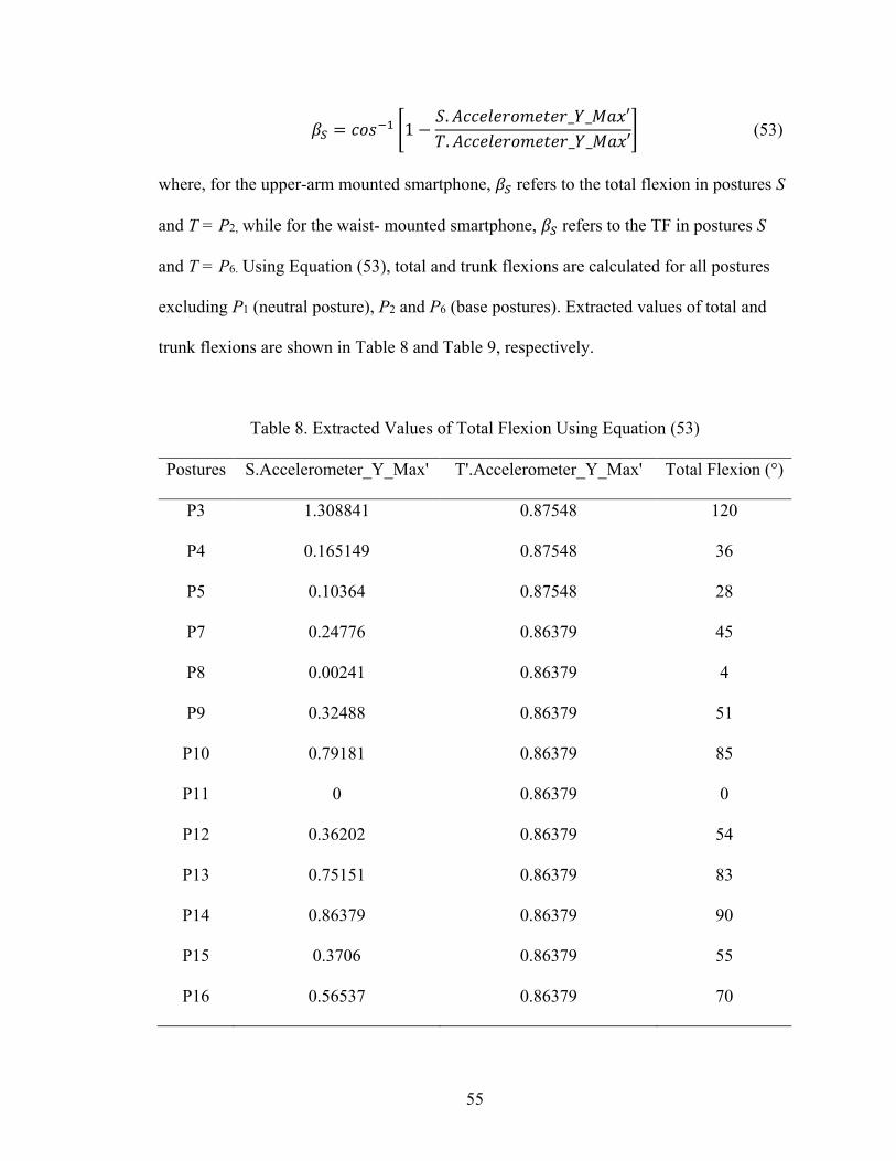
55
𝛽𝑆 = 𝑐𝑜𝑠
−1 [1 −𝑆. 𝐴𝑐𝑐𝑒𝑙𝑒𝑟𝑜𝑚𝑒𝑡𝑒𝑟_𝑌_𝑀𝑎𝑥′
𝑇. 𝐴𝑐𝑐𝑒𝑙𝑒𝑟𝑜𝑚𝑒𝑡𝑒𝑟_𝑌_𝑀𝑎𝑥′] (53)
where, for the upper-arm mounted smartphone, 𝛽𝑆 refers to the total flexion in postures S
and T = P2, while for the waist- mounted smartphone, 𝛽𝑆 refers to the TF in postures S
and T = P6. Using Equation (53), total and trunk flexions are calculated for all postures
excluding P1 (neutral posture), P2 and P6 (base postures). Extracted values of total and
trunk flexions are shown in Table 8 and Table 9, respectively.
Table 8. Extracted Values of Total Flexion Using Equation (53)
Postures S.Accelerometer_Y_Max' T'.Accelerometer_Y_Max' Total Flexion (°)
P3 1.308841 0.87548 120
P4 0.165149 0.87548 36
P5 0.10364 0.87548 28
P7 0.24776 0.86379 45
P8 0.00241 0.86379 4
P9 0.32488 0.86379 51
P10 0.79181 0.86379 85
P11 0 0.86379 0
P12 0.36202 0.86379 54
P13 0.75151 0.86379 83
P14 0.86379 0.86379 90
P15 0.3706 0.86379 55
P16 0.56537 0.86379 70

56
Table 9. Extracted Values of TF Using Equation (53)
Postures S.Accelerometer_Y_Max' T'.Accelerometer_Y_Max' Trunk Flexion (°)
P3 0 -0.429688294 0
P4 0 -0.429688294 0
P5 -0.070036067 -0.429688294 33
P7 0 -0.162001 0
P8 -0.02601 -0.162001 33
P9 -0.023402 -0.162001 31
P10 -0.040798 -0.162001 42
P11 -0.019325 -0.162001 28
P12 -0.042532 -0.162001 42
P13 -0.046578 -0.162001 45
P14 -0.025291 -0.162001 32
P15 -0.024317 -0.162001 32
P16 -0.162001 -0.162001 90
Next, SF values are calculated using Equation (49). Extracted and observed TF
and SF values are summarized in Table 10. As listed in Table 10 with a few exceptions,
values calculated from the hypothesis are very close to the observation-based
measurements. In particular, for posture P3, P5, P7, P9, P12, P13, and P16 measurements of
trunk and shoulder flexions by both approaches are either identical or within ±3° of the
true values. For some postures, such as P4, P8, P10, P14, and P15, the differences between
extracted and observed values are slightly higher, but still ≤ 7°. There is only one posture
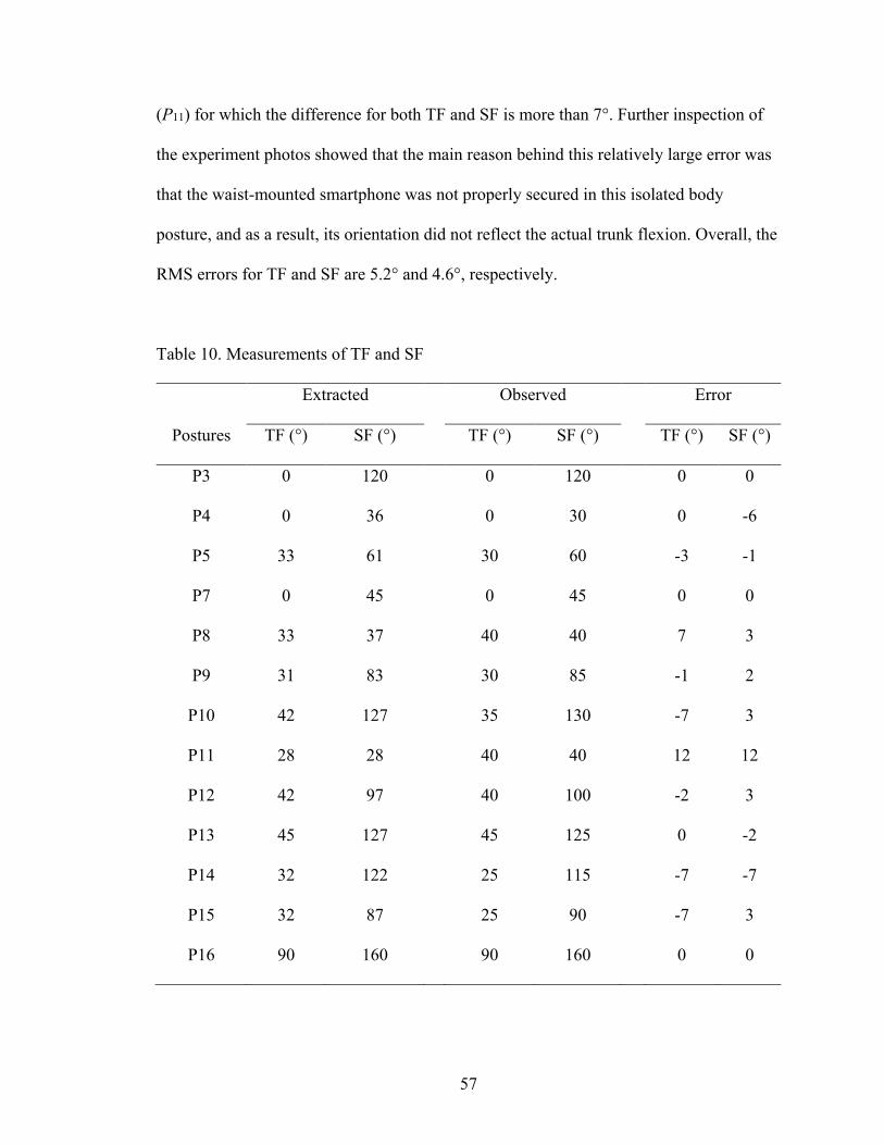
57
(P11) for which the difference for both TF and SF is more than 7°. Further inspection of
the experiment photos showed that the main reason behind this relatively large error was
that the waist-mounted smartphone was not properly secured in this isolated body
posture, and as a result, its orientation did not reflect the actual trunk flexion. Overall, the
RMS errors for TF and SF are 5.2° and 4.6°, respectively.
Table 10. Measurements of TF and SF
Postures
Extracted Observed Error
TF (°) SF (°) TF (°) SF (°) TF (°) SF (°)
P3 0 120 0 120 0 0
P4 0 36 0 30 0 -6
P5 33 61 30 60 -3 -1
P7 0 45 0 45 0 0
P8 33 37 40 40 7 3
P9 31 83 30 85 -1 2
P10 42 127 35 130 -7 3
P11 28 28 40 40 12 12
P12 42 97 40 100 -2 3
P13 45 127 45 125 0 -2
P14 32 122 25 115 -7 -7
P15 32 87 25 90 -7 3
P16 90 160 90 160 0 0

58
Errors between extracted and observed values for TF and SF are shown in Figure
11. Figure 11 shows that with one exception (P11), extracted flexions for all postures are
very close to the observed values.
Figure 11. Errors in Measurement of TF and SF
Figure 12 is a comparison between extracted and observed postures, simulated as
3D models. According to this Figure, for postures P3, P5, P7, P9, P13, and P16, extracted
and observed postures are almost identical.
0
20
40
60
80
100
120
140
160
P3 P4 P5 P7 P8 P9 P10 P11 P12 P13 P14 P15 P16
Fle
xio
ns
(deg
ree)
Extracted Trunk Flexion Extracted Shoulder Flexion

59
Figure 12. Comparison of Extracted and Observed Postures Using 3D Models
Measurement of Ergonomic Risk Levels
The ergonomic risk level of each posture is shown in Table 11. For TF of each
posture, a risk score ranging from 1 to 4 is given based on the value falling into one of the
category sizes described in Table 3. Similarly, for SF of each posture, a risk score ranging
from 1 to 5 is given. The total risk score for each posture is then calculated by adding TF
and SF risk scores, resulting in the lowest possible score of 2 and the highest possible
score of 9. Next, ergonomic risk levels of low (L), medium (M), or high (H) is assigned
to each posture based on the total risk score being 2 to 3, 4 to 6, and 7 to 9, respectively.
Table 11 shows that for 14 out of the 16 postures, risk levels calculated from the
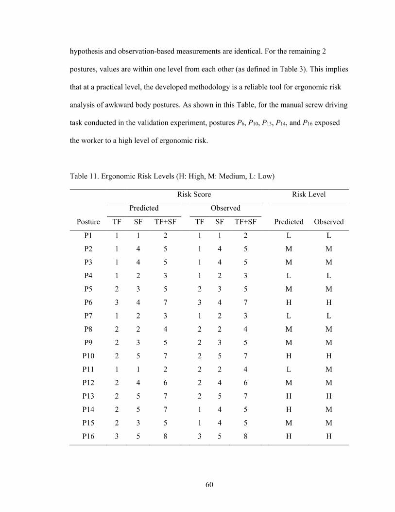
60
hypothesis and observation-based measurements are identical. For the remaining 2
postures, values are within one level from each other (as defined in Table 3). This implies
that at a practical level, the developed methodology is a reliable tool for ergonomic risk
analysis of awkward body postures. As shown in this Table, for the manual screw driving
task conducted in the validation experiment, postures P6, P10, P13, P14, and P16 exposed
the worker to a high level of ergonomic risk.
Table 11. Ergonomic Risk Levels (H: High, M: Medium, L: Low)
Risk Score Risk Level
Predicted Observed
Posture TF SF TF+SF TF SF TF+SF Predicted Observed
P1 1 1 2 1 1 2 L L
P2 1 4 5 1 4 5 M M
P3 1 4 5 1 4 5 M M
P4 1 2 3 1 2 3 L L
P5 2 3 5 2 3 5 M M
P6 3 4 7 3 4 7 H H
P7 1 2 3 1 2 3 L L
P8 2 2 4 2 2 4 M M
P9 2 3 5 2 3 5 M M
P10 2 5 7 2 5 7 H H
P11 1 1 2 2 2 4 L M
P12 2 4 6 2 4 6 M M
P13 2 5 7 2 5 7 H H
P14 2 5 7 1 4 5 H M
P15 2 3 5 1 4 5 M M
P16 3 5 8 3 5 8 H H

61
Summary and Conclusions
Since awkward posture is a major risk factor that can lead to WMSDs, this
Chapter primarily focused on assessing ergonomic risk levels associated with awkward
postures. Generally, for awkward postures, risk levels are evaluated by measuring
deviation angles of various body parts. In this research, trunk flexion (TF) and shoulder
flexion (SF) were considered. In particular, it was hypothesized that if an arbitrary
posture could be expressed as a weighted composition of base postures, then any feature
of that posture would also be a weighted composition of the corresponding features of the
base postures. Furthermore, the weight factors in the feature composition are functions of
corresponding weights for the posture composition. Based on this hypothesis, an equation
was developed to measure TF and SF using smartphone’s built-in sensors. In order to
validate the developed hypothesis, an experiment was conducted with mounting two
smartphones on a worker’s body; one on the upper-arm and another on the waist. Data
from the smartphones’ sensors were collected while the worker was performing a manual
screw driving task under different body postures. Collected data were processed into
distinctive features, and it was found that for the specific experiment carried out in this
research, the Accelerometer_Y_Max feature was the best feature for predicting flexions.
Therefore, this feature was ultimately selected for predicting TF and SF values. Results
indicated that extracted values based on the hypothesis were very close to the
observation-based measurements. Therefore, the proposed methodology could be reliably
used to assess the ergonomic risk levels associated with awkward postures. It must be
noted that the developed methodology and analysis can be also generalized with slight
modification to measure angles of other body parts, and for different classes of field

62
activities including both static and dynamic tasks. Moreover, promising results obtained
from the designed methodology and field experiments indicate that a similar approach
can be adapted and used to assess ergonomic risk levels of a wider range of activities in
different occupations including manufacturing, carpentry, welding, farming, operating
tools or machinery, athletics, and office work.

63
MACHINE LEARNING IN HUMAN ACTIVITY RECOGNITION
In order to better illustrate the meaning of machine learning, let’s borrow from the
example of a game of checkers. Imagine a computer program made of thousands of
embedded lines of code that allow a user to play checkers. While this program may
outperform a human user, it can hardly be considered as “intelligent” since all it does is
to blindly follow a predetermined set of rules, scenarios, and instructions. Now, imagine
a modified version of that same program which can “learn” how to play checkers by
observing (in technical terms, by analyzing the data from) millions of real games and
improving its ability over time by playing and responding to more complex user
movements. This new version can be technically deemed intelligent. Interestingly, the
idea of such learning by a manmade machine dates back to 1959 when Arthur Samuel
wrote that famous checkers playing program in an early IBM computer and coined the
term “machine learning” (McCarthy & Feigenbaum, 1990).
Machine learning is an essential step for artificial intelligence (AI) since it enables
machines to learn rules and concepts based on observing examples or by analyzing data,
ultimately perform tasks that rely on complex analysis and subtle judgement (Manyika et
al., 2013). Through the use of machine learning, machines no longer simply rely on fixed
(predetermined) algorithms and rules provided by the programmers; rather they can
modify their own algorithms and reasoning processes based on real data, enabling them
to find hidden rules and patterns that human programmers might overlook (Manyika et
al., 2013). Moreover, the more data a machine processes, the more it learns and the
smarter it gets. Machine learning has been identified by Accenture as the most trending

64
technology of 2016 (Daugherty, Carrel-Billiard, & Blitz, 2016), and is considered as one
of the most disruptive recent technologies by the McKinsey Global Institute (MGI)
(Manyika et al., 2013).
Machine Learning
Definitions. Machine learning is defined by Arthur Samuel as “the computer’s
ability to learn something without being explicitly programmed” (Das, Dey, Pal, & Roy,
2015). A more formal definition is given by Tom Mitchel (2006); a machine learns from
its experience E with respect to a particular task T and a performance metric P, if it
consistently improves its performance P at task T, following the experience E. In the
checker-playing computer program described earlier, T, P, and E are playing checkers
(i.e. task), the probability to win against an opponent (i.e. performance), and playing
millions of games against itself (i.e. experience), respectively. It should be noted that
depending on the specification of T, P, and E, other terms may be interchangeably used to
describe machine learning including data mining, statistical learning, autonomous
discovery, database updating, and programming by example (Mitchell, 2006). In this
Thesis, the term machine learning is used synonymously with data mining. In particular,
when machine learning is applied to a collection of data it is referred to as data mining.
From this perspective, machine learning (or data mining) can be defined as a non-trivial
process of identifying valid, potentially useful, and ultimately understandable patterns or
information in large amounts of data (Murphy, 2012; Sumathi & Sivanandam, 2006).
Supervised vs. Unsupervised Learning. In a broader scheme, machine learning
can be divided into two categories of supervised learning and unsupervised learning
65
(Dunham, 2006). In supervised learning, machine learns from examples, i.e., from given
datasets and correct answers (Dunham, 2006). Supervised learning can be further divided
into two categories, classification and regression (Harrington, 2012). In classification, the
output values are categorical, e.g., colors and activities. On the other hand, in regression,
the output values are continuous and numerical, e.g., age and temperature. Supervised
learning has been widely used in spam filtering, handwriting, face, speech, and human
activity recognition (HAR), information retrieval, natural language processing, and
computer vision (Das et al., 2015). In unsupervised learning, on the other hand, there is
only inputs, without any output. The overall goal of this class of machine learning
algorithms is to partition the input set X into subsets X1, X2, …, Xn in some meaningful
manner (Nilsson, 1996). Unsupervised learning is extensively used in applications such
as extracting genome sequence from DNA, social network analysis, market analysis,
anomaly detection in astronomy, medical diagnosis, and computational biology (Das et
al., 2015). In this Thesis, machine learning is used for HAR which falls under the
category of supervised learning, more specifically, classification. The key idea for using
machine learning in this research is to utilize this tool to recognize construction workers’
activities on a jobsite, and to evaluate ergonomic risks associated with such activities.
The detailed methodology of ergonomic analysis will be discussed in the next Chapter. In
this Chapter, various classification algorithms and their performance for the specific
purpose of HAR are discussed.

66
Classification
As mentioned earlier, classification falls under the category of supervised learning
which deals with the outputs of categorical (i.e. discrete) variables. Classification is one
of the most popular machine learning techniques that has been used in a variety of
domains. Application of classification includes but not limited to image, pattern and face
recognition, medical diagnosis, loan approval, classifying financial market trends, and
spam filtering (Das et al., 2015; Dunham, 2006).
Key Terminology. To understand the key terminology used in classification,
consider an example of HAR. Assume, a classification task that is to classify human
activities based on several measurable parameters (e.g. name, gender, mean of
accelerometer’s X- and Y- readings), as shown in Figure 13. These parameters are called
features (a.k.a. attributes) and usually presented as columns in a dataset (Figure 13).
Each row shown in the table in Figure 13 is called an instance (a.k.a. tuple, data point,
observation, item, example and record). In this specific example, one instance represents
one time window. The goal of this particular classification problem is to output the name
of the activity for each instance based on the feature values of that instance. In
classification, outputs are known as classes (i.e., activities, in this example). It should be
noted that in a classification problem, features can be numerical (i.e. real numbers),
binary (e.g. yes-no or 1-0), or categorical (i.e. enumeration or having fixed number of
possible values). In this example, as shown in Figure 13, Acc-x-mean and Acc-Y-mean are
numerical features, Gender is a binary feature, and Name is a categorical feature. Similar
to other classification problems, in this example, the class, i.e., activity, is a categorical

67
variable. In practice, often numerical features are used in HAR, and quantitatively more
number of features are used than what has been demonstrated in this example.
Figure 13. Key Terminology in HAR Classification Example
Mathematical Definition. Given a dataset 𝐷 = {𝐼1, 𝐼2, … , 𝐼𝑛} consisting of n
number of instances and a set of predefined classes C = {𝐶1, 𝐶2, … , 𝐶𝑚}, the classification
problem is to define a mapping function 𝑓: 𝐷 → 𝐶 where each 𝐼𝑖 is assigned to one class
𝐶𝑗 (Dunham, 2006). A class 𝐶𝑗 contains precisely those instances that are mapped to it
(Dunham, 2006), as mathematically shown in Equation (54).
𝐶𝑗 = {𝐼𝑖| 𝑓(𝐼𝑖) = 𝐶𝑗 , 1 ≤ 𝑖 ≤ 𝑛 𝑎𝑛𝑑 𝐼𝑖 ∈ 𝐷 } (54)
It must be noted that classes are non-overlapping (i.e. each instance is assigned to
exactly one class) and partition the entire database (Dunham, 2006). Mathematically, this
can be expressed by intersection and union operators of Equation (55).
𝐶𝑖 ∩ 𝐶𝑗 = ∅ 𝑖𝑓 𝑖 ≠ 𝑗, 𝑎𝑛𝑑 ⋃𝐶𝑖 = 𝐷
𝑚
𝑖=1
(55)

68
Implementation. The core “machine learning” in classification takes place in two
phases: training and testing (Dunham, 2006; Harrington, 2012). During the training
phase, the dataset contains defined class labels for each instance and is referred to as the
training dataset. In this phase, a classification algorithm (a.k.a. classifier) takes training
dataset as input and outputs a model for future classification (a.k.a. prediction). In the
testing phase, the dataset contains no information about the classes, i.e., it consists of
only the matrix of features and instances, and known as the testing dataset. In this phase,
the model, developed in the training phase, is applied to the testing dataset and prediction
of class for each instance of the testing dataset is recorded. The testing phase is very
straightforward to implement. However, much efforts should be put in the training phase
to build the best model that would deliver adequate performance.
Classifier Algorithms
Classification algorithms can be grouped into the following major categories
(Dunham, 2006):
• Statistical
• Decision tree
• Distance algorithm
• Neural network
• Rule-based algorithms
In this Section, several commonly used classifier algorithms are discussed. These
algorithms mainly fall under the first four of the aforementioned categories.

69
Naïve Bayes. Naïve Bayesian (NB) classifier (a.k.a. Simple Bayesian classifier) is
a statistical-based algorithm. It uses probabilistic model based on the Bayes Theorem and
the assumption that the effect of an attribute value on a given class is independent of the
effect of other values (a.k.a. conditional independence) (Dunham, 2006). Given a test
instance X, the class corresponding to X among k existing classes C1, C2, C3…Ck, is
predicted by calculating the highest conditional probability 𝑃(𝐶𝑖|𝑋) for 1 ≤ i ≤ k. These
probabilities are computed using Bayes theorem which is shown in Equation (56),
𝑃(𝐶𝑖|𝑋) =
𝑃(𝑋|𝐶𝑖). 𝑃(𝐶𝑖)
𝑃(𝑋)
(56)
As the computation of 𝑃(𝐶𝑖|𝑋) can be difficult, the naïve assumption of conditional
independence between attributes is made to simplify the computation. Using this
assumption, if the instance X has n different features denoted by {𝑥1, 𝑥2, … , 𝑥𝑛}, the
conditional probability that X belongs to class Ci, i.e., 𝑃(𝑋|𝐶𝑖), can be calculated by
Equation (57),
𝑃(𝑋|𝐶𝑖) = ∏𝑃(𝑥𝑗|𝐶𝑖)
𝑛
𝑗=1
(57)
In theory, the NB classifier should yield the minimum error compared to other
methods. But, in practice, this may not be always the case given the noise in data and the
assumptions made by the method to simplify the computation (Dunham, 2006).
Decision Tree. Decision tree (DT) is one of the most powerful yet simplest
algorithms for classification and its major advantage is ease of use and human
interpretability (Bishop, 2006). The DT method used in this Thesis is often referred to as
standard Classification and Regression Trees (CART) (variants include ID3 and C4.5).

70
The CART algorithm performs recursive binary partitioning of the input feature space
(i.e. dividing the entire feature space into two regions, recursively subdividing each sub-
region into two further sub-regions until a stopping criterion is met), and assigning each
class to a final sub-region (a.k.a. leaf node) (Bishop, 2006). The algorithm follows a
greedy optimization technique to select the best split by examining all possible candidate
regions in the feature space. The optimization criterion used in this research is an
entropy-based measurement called the Gini index (a.k.a. Gini diversity index), which is
shown in Equation (58),
𝐺. 𝐼. (𝑇) = 1 − ∑𝑝𝑇𝑖2
𝑘
𝑖=1
(58)
where, 𝐺. 𝐼. (𝑇) is the Gini index at node T, and 𝑝𝑇𝑖 is the observed fraction of instances
labeled with class i at node T. The Gini index is a measure of node impurity. A node is
considered pure if it has only one class, i.e. Gini index of zero (Akhavian, 2015). The
stopping criteria for the algorithm used in this research are based on the number of
branch nodes (i.e. parent of the leaf nodes) and the number of instances in the branch and
leaf nodes.
K-nearest Neighbor. Similar to DT, the K-nearest neighbor (KNN) is also a
simple algorithm. The algorithm uses the entire training data, including the feature space
and defined class for each instance, as the model (Dunham, 2006). For classifying a new

71
instance, the algorithm finds its k closest instances (a.k.a. nearest neighbors) in the model
(i.e. training data) and the class is assigned to the new instance based on the majority
vote, i.e., the class that contains majority of the k nearest neighboring instances
(Harrington, 2012). To find the nearest neighbors, a distance-based measurement (i.e.
Euclidian distance in this research) is used similar to what is shown in Equation (59),
𝑑𝑖𝑠𝑡(𝐼𝑛𝑒𝑤, 𝐼𝑖) = √∑(𝑥𝑛𝑒𝑤,𝑗 − 𝑥𝑖,𝑗)2
𝑚
𝑗=1
(59)
where, 𝑑𝑖𝑠𝑡(𝐼𝑛𝑒𝑤, 𝐼𝑖) is the Euclidian distance between new instance 𝐼𝑛𝑒𝑤 and an
instance 𝐼𝑖 from the training dataset, and 𝑥𝑛𝑒𝑤,𝑗 and 𝑥𝑖,𝑗 are features of 𝐼𝑛𝑒𝑤 and 𝐼𝑖,
respectively, in the jth dimension of the m-dimensional feature space. In this research, all
features are standardized using Equation (60). Here, z is the standardized value of x, and
μ and σ are mean and standard deviation, respectively. Mathematically, μ and σ can be
calculated using Equation (7) and Equation (8), respectively.
𝑧 =𝑥 − 𝜇
𝜎 (60)
Artificial Neural Network. Similar to human brain, artificial neural network
(ANN) is composed of many neurons (a.k.a. nodes). In ANN, each neuron works
independently and uses local data consisting of inputs on the node, edges going into the
node, weights on the edges and a processing function (a.k.a. activation function) for the
node (Dunham, 2006). As shown in Figure 14, each node in the input layer represents one
feature in the feature space, and each node in the output layer represents one class. In this

72
Thesis, the Backpropagation (BP) algorithm is used which performs learning on a feed-
forward multilayer perceptron (MLP). A node is connected to every node in the next layer
(Figure 14) and training is processed by adjusting the weights on the edges. A sigmoid
function is usually used in BP even though other functions could be used. An example of
a sigmoid function is shown in Equation (61), where, C is a constant.
ℎ(𝑥) =
1
1 + 𝑒−𝐶𝑥
(61)
Figure 14. Multilayer Neural Network
Support vector machine. Support vector machine (SVM) is considered a
relatively more powerful classifier algorithm compared to DT and KNN, and has been
widely used in vision-based pattern recognition and classification of human activities
(Akhavian, 2015). The key idea of SVM is to separate the instances of two classes in the

73
n-dimensional feature space by a (n-1)-dimensional plane, called the separating
hyperplane (a.k.a. decision boundary) (Harrington, 2012). SVM can utilize kernel
function to create nonlinear classifiers by maximizing the margin along the hyperplane in
a transformed feature space (Akhavian, 2015). In this research, several kernel functions
are used including linear, polynomial (e.g. quadratic and cubic) and Gaussian function
(a.k.a. radial basis function, RBF). A linear kernel function is shown in Equation (62),
𝐾(𝑥1, 𝑥2) = 𝑥1𝑇𝑥2 (62)
where, 𝑥1 and 𝑥2 are two vectors in the input feature space, and 𝑥1𝑇𝑥2 represents the
inner product of the two vectors. With similar notation, polynomial kernel function can
be expressed by Equation (63), where p is the order of the polymodal (e.g. for quadratic
function, p = 2, and for cubic function, p = 3),
𝐾(𝑥1, 𝑥2) = (1 + 𝑥1𝑇𝑥2)
𝑝 (63)
The Gaussian function (i.e. RBF) can be expressed as shown in Equation (64),
where, 𝜎 is a user-defined parameter, and ||𝑥1 − 𝑥2|| represents the Euclidian distance
between two vectors 𝑥1 and 𝑥2.
𝐾(𝑥1, 𝑥2) = 𝑒𝑥𝑝 (
−||𝑥1 − 𝑥2||2
2𝜎2)
(64)
It must be noted that SVM deals with two classes at a time. For multi-class
classification, in this research, the one-vs-one method is used which performs binary
classification for all possible combinations of class pairs. For example, for k classes,
multi-class SVM builds k(k-1)/2 binary classifiers.

74
Logistic regression. In logistic regression (LR), the output is discretized for
classification, and it forms a hypothesis function that maps the input (i.e. training data) to
the output (i.e. class labels) by approximating the conditional probability of an instance
that belongs to class k, given the condition that the instance actually belongs to class k
(Akhavian, 2015). The algorithm minimizes a cost function using the hypothesis function
and the correct classes to find the parameters of a mapping model (Friedman, Hastie, &
Tibshirani, 2001). The hypothesis function used in this research is logistic function (a.k.a.
sigmoid function) and it is similar to the processing function introduced in Equation (61).
The cost function is shown in Equation (65),
𝐽(θ) = −
1
𝑚∑[𝑌𝑖𝑙𝑜𝑔{ℎθ(𝑋𝑖)} + (1 − 𝑌𝑖)𝑙𝑜𝑔{1 − ℎθ(𝑋𝑖)}]
𝑚
𝑖=1
(65)
where, 𝐽(𝜃) is the cost function for the mapping model 𝜃, 𝑋𝑖 is one instance from the m
training data points, 𝑌𝑖 is its class label, and ℎθ(𝑋𝑖) is the hypothesis function. In this
research, the cost function is minimized using Quasi-Newton method to optimize the
parameters. Similar to SVM, LR deals with binary classes. For multi-class classification,
the one-versus-all method is used, i.e., for each of the k classes, the hypothesis function is
evaluated considering whether or not a new instance belongs to the corresponding class
(Friedman et al., 2001). Finally, the class with maximum value for hypothesis function is
selected (Akhavian, 2015).
75
Evaluation of Classifier Performance
In the previous Section, several classifier algorithms were described. In practice,
the performance of different classifier algorithms varies significantly depending on the
quality and nature of the training and test datasets (Friedman et al., 2001). Therefore, it is
important that for a particular task, the performance of these algorithms is first evaluated
before the best classifier can be selected for prediction (Friedman et al., 2001).
Researchers have been using various measures for evaluating the performance of
classifier models. In general, all performance measures are based on how well a model
can predict the classes of input instances. To compare the prediction of the model with
the actual results, in practice, a portion of the training dataset is used as a test dataset.
Generally, if the training dataset is large enough, it is split into two uneven portions. The
larger portion is used to train the classifier model, while the smaller is used to evaluate
the performance of the model in prediction. However, for relatively small training
datasets, splitting the data in such a way further reduces the size of the training dataset
and increases the chance of overfitting (Nilsson, 1996), a condition that occurs when the
built model fits the present states too well, but does not fit the future states (Dunham,
2006). Therefore, in such cases, it is more practical to use a technique that is referred to
as cross-validation. In cross-validation, the training dataset T is divided into k equally-
sized, mutually exclusive, and exhaustive subsets 𝑇1, 𝑇2, … , 𝑇𝑘 (Nilsson, 1996). For each
subset 𝑇𝑖, the model is trained on the rest of the training dataset, i.e., 𝑇 − 𝑇𝑖, and the
performance of the model is tested on the 𝑇𝑖 subset (Nilsson, 1996). Finally, all of the k-
fold performances are combined to report the overall performance of the model. This
method is also known as k-fold cross-validation.

76
Performance Metrics
In previous Section, the discussion was based on how to prepare the training
dataset to evaluate the performance of a classifier model. In this Section, a brief
description of the most commonly used mathematical approaches to measure the
performance of classification algorithms is provided (Sokolova & Lapalme, 2009).
Accuracy and Error Rate. The simplest way to measure the performance of a
classifier model is to calculate the percentage of instances that have been correctly
classified by the model (i.e. accuracy) (Dunham, 2006). In mathematical terms, this can
be expressed by Equation (66).
𝐴𝑐𝑐𝑢𝑟𝑎𝑐𝑦 = 𝑁𝑜. 𝑜𝑓 𝑖𝑛𝑠𝑡𝑎𝑛𝑐𝑒𝑠 𝑐𝑜𝑟𝑟𝑒𝑐𝑡𝑙𝑦 𝑐𝑙𝑎𝑠𝑠𝑖𝑓𝑖𝑒𝑑
𝑇𝑜𝑡𝑎𝑙 𝑛𝑜. 𝑜𝑓 𝑖𝑛𝑠𝑡𝑎𝑛𝑐𝑒𝑠×100%
(66)
Alternately, another way to present the accuracy measure is the error rate which
refers to the percentage of misclassified instances, and can be expressed as shown in
Equation (67),
𝐸𝑟𝑟𝑜𝑟 𝑟𝑎𝑡𝑒 = 𝑁𝑜. 𝑜𝑓 𝑖𝑛𝑠𝑡𝑎𝑛𝑐𝑒𝑠 𝑖𝑛𝑐𝑜𝑟𝑟𝑒𝑐𝑡𝑙𝑦 𝑐𝑙𝑎𝑠𝑠𝑖𝑓𝑖𝑒𝑑
𝑇𝑜𝑡𝑎𝑙 𝑛𝑜. 𝑜𝑓 𝑖𝑛𝑠𝑡𝑎𝑛𝑐𝑒𝑠×100%
= 100%− 𝐴𝑐𝑐𝑢𝑟𝑎𝑐𝑦 (67)
Confusion Matrix. The error rate (or accuracy) represents the overall
performance of a classifier model, but it does not provide any information on how
instances are misclassified (Harrington, 2012). A better way to present such information
is through the use of a confusion matrix. A confusion matrix is a m-by-m matrix for a m-
class classification problem, in which rows represent the actual classes, and columns
represent the predicted classes. Thus, the cell (i, j) in a confusion matrix represents the
number (or percentage) of instances that actually belong to class i, but were predicted by

77
the model to belong to class j. Using this definition, in a confusion matrix, as shown in
Figure 15, diagonal cells (i.e. 𝑖 = 𝑗) represent correctly classified instances, while non-
diagonal cells (i.e. 𝑖 ≠ 𝑗) represent misclassified instances. This provides a better
understanding of the classification error (Harrington, 2012) because it shows how a
classifier model confuses instances of one class with those of another classes.
Figure 15. Confusion Matrix for a Three-class Classification Example
Precision and Recall. The previously mentioned performance measures ignore
the fact that there might be a cost associated with the misclassification (Dunham, 2006).
For example, in medical diagnosis, if a classifier model predicts a cancerous tumor to be
non-cancerous, it is more dangerous than if the model predicts a non-cancerous tumor to
be cancerous; because the former prediction puts the life of the patient at risk. To
overcome this issue, precision (a.k.a. confidence) and recall (a.k.a. sensitivity) are
calculated which are more sensitive to the error of classification. To understand these
measures, consider the confusion matrix of a binary-class problem which is shown in
Figure 16. Following the notation presented in Figure 16, precision is the fraction of
Actual class A
Predicted class A A
Actual class A
Predicted class B
Actual class A
Predicted class C
Actual class B
Predicted class A B
Actual class B
Predicted class B
Actual class B
Predicted class C
Actual class C
Predicted class A C
Actual class C
Predicted class B
Actual class C
Predicted class C
A B C
Predicted Class
Actual Class
Correctly classified Misclassified

78
predicted positive instances (i.e. TP + FP) that are truly positive (TP), while recall refers
to the fraction of true instances (i.e. TP + FN) that are correctly predicted as positive (TP)
(Powers, 2011). Mathematically, precision and recall can be expressed by Equations (68)
and (69), respectively.
𝑃𝑟𝑒𝑐𝑖𝑠𝑖𝑜𝑛 =
𝑇𝑃
𝑇𝑃 + 𝐹𝑃
(68)
𝑅𝑒𝑐𝑎𝑙𝑙 =
𝑇𝑃
𝑇𝑃 + 𝐹𝑁
(69)
Figure 16. Confusion Matrix of a Binary-Class Classification Example
F-measure. While it may be desirable to achieve a high precision or recall for a
classification model, it is often challenging to maximize both measures for a single model
(Harrington, 2012). One solution is to tradeoff one measure for another depending on the
classification task (Buckland & Gey, 1994). Mathematically, this can be done using the
F-measure (a.k.a. F-score) which is formulated in Equation (70),
𝐹𝛽 = (1 + 𝛽2)
𝑃𝑟𝑒𝑐𝑖𝑠𝑖𝑜𝑛×𝑅𝑒𝑐𝑎𝑙𝑙
𝛽2×𝑃𝑟𝑒𝑐𝑖𝑠𝑖𝑜𝑛 + 𝑅𝑒𝑐𝑎𝑙𝑙
(70)
True Positive
(TP) A
False Negative
(FN)
False Positive
(FP)
Not
A
True Negative
(TN)
A Not A
Predicted Class
Actual Class

79
where, 𝐹𝛽 is the F-measure (the measure of effectiveness), and 𝛽 is a user-defined
constant which indicates the importance of recall compared to precision (Sasaki, 2007).
For example, if precision and recall are both equally important for a particular scenario,
𝛽 = 1 is selected. Thus, the F-measure 𝐹1 is the harmonic mean of precision and recall,
as shown in Equation (71),
𝐹1 = 2×𝑃𝑟𝑒𝑐𝑖𝑠𝑖𝑜𝑛×𝑅𝑒𝑐𝑎𝑙𝑙
𝑃𝑟𝑒𝑐𝑖𝑠𝑖𝑜𝑛 + 𝑅𝑒𝑐𝑎𝑙𝑙
(71)
Relative Operating Characteristic Curve. The relative operating characteristic
(ROC) curve is a graphical representation of the relationship between true and false
positives, as shown in Figure 17 (Dunham, 2006).
Figure 17. ROC Curves for Ideal, Normal, and Random-Guessing Classifiers

80
In this Figure, the horizontal axis of the ROC curve is the false positive rate,
while the vertical axis is the true positive rate. For a good classifier, the ROC curve
should be in the upper-left of the graph as much as possible (Harrington, 2012). For
quantitative comparison among ROC curves of different classifiers, generally the area
under the curve (AUC) is measured (Harrington, 2012). As shown in Figure 17, an ideal
classifier would have an AUC of 1.0, while for random guessing, this value would be 0.5.
Software Implementation
In this research, classifier algorithms are applied to collected data and
performance metrics are calculated using two primary software packages, MATLAB and
Weka. In particular, NB, DT, KNN, and SVM algorithms are implemented using
MATLAB’s predefined functions, and ANN and LR algorithms are implemented by
calling Weka functions from MATLAB’s interface. A list of all implemented functions is
given in Table 12.
Table 12. Built-in Functions for Applying Classifier Algorithms
Software Algorithm Function
MATLAB NB fitcnb
DT fitctree
KNN fitcknn
SVM templateSVM,fitcecoc
WEKA ANN MultilayerPerceptron
LR Logistic
81
A detailed discussion about the functions listed in Table 12 is out of the scope of
this Thesis, and can be found in MathWorks (MathWorks, 2017) and Weka (Weka,
2017). An example of a piece of MATLAB code used to implemented the KNN
algorithm is given in the following lines.
% Building KNN classifier model
mdl = fitcknn(Xtrain,Ytrain);
trainedKNN.Classifier = mdl;
test = @(x) predict(mdl, x);
trainedKNN.predictFcn = @(x) test(predictorExtractionFcn(x));
% Performing 5-fold cross-validation
cvmdl = crossval(trainedKNN.Classifier, 'KFold', 5);
% Computing validation accuracy
acc = 1 - kfoldLoss(cvmdl, 'LossFun', 'ClassifError');
% Predictions of the trained model on testing dataset
Ytest = trainedKNN.test(Xtest);
Classification of Human Activities
As described at length in previous Chapters, the subject of HAR using wearable
sensors has been undergoing intensive research for several years, especially, with the
rapid advancement of mobile sensing technologies. Particularly, machine learning tools
have been widely used as an integral component of HAR (Lara & Labrador, 2013). The
key idea of utilizing machine learning, (and more specifically, classification algorithms)
in HAR is to recognize human activities from distinguishable patterns in time-motion
data extracted from wearable sensors (i.e. smartphone’s motion sensors in this Thesis).
Within the context of classification for HAR, given extracted statistical features (e.g.
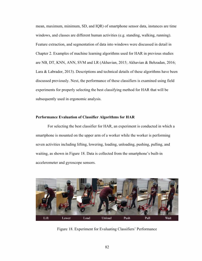
82
mean, maximum, minimum, SD, and IQR) of smartphone sensor data, instances are time
windows, and classes are different human activities (e.g. standing, walking, running).
Feature extraction, and segmentation of data into windows were discussed in detail in
Chapter 2. Examples of machine learning algorithms used for HAR in previous studies
are NB, DT, KNN, ANN, SVM and LR (Akhavian, 2015; Akhavian & Behzadan, 2016;
Lara & Labrador, 2013). Descriptions and technical details of these algorithms have been
discussed previously. Next, the performance of these classifiers is examined using field
experiments for properly selecting the best classifying method for HAR that will be
subsequently used in ergonomic analysis.
Performance Evaluation of Classifier Algorithms for HAR
For selecting the best classifier for HAR, an experiment is conducted in which a
smartphone is mounted on the upper arm of a worker while the worker is performing
seven activities including lifting, lowering, loading, unloading, pushing, pulling, and
waiting, as shown in Figure 18. Data is collected from the smartphone’s built-in
accelerometer and gyroscope sensors.
Figure 18. Experiment for Evaluating Classifiers’ Performance

83
Following the methodology described in Chapter 2, collected data is segmented
into 2-second windows with 50% overlapping, and processed into 42 features. As shown
in Figure 19, for each sensor axis (X, Y, and Z) (accelerometer and gyroscope), four
statistical features, i.e., mean (Equation (7)), maximum, minimum, and IQR (Equation
(10)) are calculated.
Figure 19. Extracted Features for Data Analysis
Next, each instance of the window is labelled with the class of corresponding
activity. Next, all extracted features are ranked using the ReliefF algorithm. Assume, a
feature is denoted as 𝑓𝑟 where r is the rank of the feature determined by the ReleifF
algorithm, thus, the feature space can be written as 𝐹 = {𝑓1, 𝑓2, . . , 𝑓42}. A subset of this
feature space, 𝑅𝑛, refers to the set of best n features, i.e., {𝑓1, 𝑓2, . . , 𝑓𝑛}.
The performance of NB, ANN, and LR classifier algorithms is evaluated for one
parameter, i.e., feature subset 𝑅𝑛, where n = 1 to 42. For convention, in functional
notation, the models are denoted as 𝑁𝐵(𝑅𝑛), 𝐴𝑁𝑁(𝑅𝑛), and 𝐿𝑅(𝑅𝑛), where 𝑅𝑛 ∈
{𝑅1, 𝑅2, … , 𝑅42}. For DT, KNN, and SVM, evaluation is performed in greater extents, for
an additional parameter for each of the algorithms. For DT, the additional parameter is
Accelerometer
Gyroscope
SensorsX
Y
Z
AxesMean
Maximum
Minimum
IQR
Features

84
the number of branch nodes in the tree which is denoted as 𝛽, where 𝛽 ∈
{1, 5, 10, 25, 50, 100}. For KNN, the parameter is the number of the nearest neighbor k,
where 𝑘 ∈ {1, 5, 10, 25, 50, 100}. For SVM, the parameter is kernel function and denoted
as 𝜑. In this research, selected kernel functions for SVM are linear, quadratic, cubic, fine
Gaussian, medium Gaussian, and coarse Gaussian. For each algorithm and for n = 1 to
42, performance is measured in terms of accuracy for 5-fold cross-validation and the
highest values of the accuracies are summarized in Table 13. It can be seen that for NB,
ANN, LR, DT, KNN, and SVM, the models 𝑁𝐵(𝑅𝑛=41), 𝐴𝑁𝑁(𝑅𝑛=42), 𝐿𝑅(𝑅𝑛=37),
𝐷𝑇(𝛽 = 100, 𝑅𝑛=36), 𝐾𝑁𝑁(𝑘 = 5, 𝑅𝑛=40), and 𝑆𝑉𝑀(𝜑 = 𝑐𝑢𝑏𝑖𝑐, 𝑅𝑛=29) performed best
in the respective category. Therefore, these models are selected as the best candidates for
further evaluation.
Next, the aforementioned candidate models are investigated in detail by
calculating several performance metrics. For each activity class, precision, recall, F1 and
AUC are calculated following the one-vs-others method, i.e., the corresponding class is
considered as the positive class, while other classes are considered together as a negative
class. The precision, recall, and F1 are calculated using Equations (68), (69), and (71)
respectively. Detailed results of the performance metrics are summarized in Table 14.
Next, Performance metrics of all classes are combined together by calculating the
weighted average of each metric, as shown in Figure 20. It can be seen that the SVM
classifier outperformed all others in every performance metric. The ANN and KNN
classifiers are the second and third best classifiers, respectively. Since SVM, in particular,

85
with cubic kernel function, is found to perform best on the collected dataset in this
experiment, this algorithm is ultimately selected for HAR for ergonomic analysis.
Table 13. Performance of Different Classifiers with Different Parameters
Classifier Parameter Name
n Accuracy (%) Value
NB N/A N/A 41 75.28
ANN N/A N/A 42 91.9
LR N/A N/A 37 81.3
DT Maximum Split, β 1 42 33.77
5 42 61.31
10 25 66.69
25 27 76.21
50 29 82.16
100 36 85.37
KNN k 1 13 88.77
5 40 89.49
10 31 88.85
25 40 88.24
50 41 86.71
100 13 84.07
SVM Kernel Function, φ Linear 32 84.86
Quadratic 39 93.35
Cubic 29 94.11
Fine Gaussian 21 92.13
Medium Gaussian 29 92.73
Coarse Gaussian 41 81.21
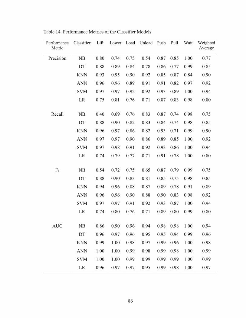
86
Table 14. Performance Metrics of the Classifier Models
Performance
Metric
Classifier Lift Lower Load Unload Push Pull Wait Weighted
Average
Precision NB 0.80 0.74 0.75 0.54 0.87 0.85 1.00 0.77
DT 0.88 0.89 0.84 0.78 0.86 0.77 0.99 0.85
KNN 0.93 0.95 0.90 0.92 0.85 0.87 0.84 0.90
ANN 0.96 0.96 0.89 0.91 0.91 0.82 0.97 0.92
SVM 0.97 0.97 0.92 0.92 0.93 0.89 1.00 0.94
LR 0.75 0.81 0.76 0.71 0.87 0.83 0.98 0.80
Recall NB 0.40 0.69 0.76 0.83 0.87 0.74 0.98 0.75
DT 0.88 0.90 0.82 0.83 0.84 0.74 0.98 0.85
KNN 0.96 0.97 0.86 0.82 0.93 0.71 0.99 0.90
ANN 0.97 0.97 0.90 0.86 0.89 0.85 1.00 0.92
SVM 0.97 0.98 0.91 0.92 0.93 0.86 1.00 0.94
LR 0.74 0.79 0.77 0.71 0.91 0.78 1.00 0.80
F1 NB 0.54 0.72 0.75 0.65 0.87 0.79 0.99 0.75
DT 0.88 0.90 0.83 0.81 0.85 0.75 0.98 0.85
KNN 0.94 0.96 0.88 0.87 0.89 0.78 0.91 0.89
ANN 0.96 0.96 0.90 0.88 0.90 0.83 0.98 0.92
SVM 0.97 0.97 0.91 0.92 0.93 0.87 1.00 0.94
LR 0.74 0.80 0.76 0.71 0.89 0.80 0.99 0.80
AUC NB 0.86 0.90 0.96 0.94 0.98 0.98 1.00 0.94
DT 0.96 0.97 0.96 0.95 0.95 0.94 0.99 0.96
KNN 0.99 1.00 0.98 0.97 0.99 0.96 1.00 0.98
ANN 1.00 1.00 0.99 0.98 0.99 0.98 1.00 0.99
SVM 1.00 1.00 0.99 0.99 0.99 0.99 1.00 0.99
LR 0.96 0.97 0.97 0.95 0.99 0.98 1.00 0.97

87
Figure 20. Comparison of Performance of Different Classifiers
Summary and Conclusions
Machine learning is the process in which a machine improves its performance on
a particular task by analyzing data corresponding to that task. The learning process could
be either supervised or unsupervised. In supervised learning, a machine learns from given
examples and correct answers. A particular category of supervised learning is
classification, in which the correct answers (i.e. outputs) are categorical values (a.k.a.
classes). In this process, the task is to optimize a function that maps output classes from
the given dataset.
Classification has been widely used in HAR, especially in the healthcare domain.
In a classification problem corresponding to HAR using wearable sensors, the classifier
algorithm predicts the output classes (i.e. activities) from the given dataset of instances
(i.e. time windows) and features (which are extracted from sensor readings). The most
commonly used classifier algorithms are NB, DT, KNN, ANN, SVM and LR. Since
0.7
0.75
0.8
0.85
0.9
0.95
1
Precision Recall F-1 AUC
NB DT KNN ANN SVM LR

88
performance of classifiers vary for different tasks and datasets, in this research, in order
to find the most effective algorithm for activity recognition, a field experiment was
conducted in which several field activities such as lifting, lowering, loading, unloading,
pushing, pulling, and waiting were performed and sensor readings from a smartphone
mounted on the performer’s body were recorded. The recorded data were then
transformed into features and segmented into windows. Next, the dataset was fed into
different classifier algorithms with different parameters, and the performance of
algorithms were measured in terms of accuracy, precision, recall, F1, and AUC. It was
found that the SVM algorithm with cubic kernel function performed best among all
classifiers in recognizing the activities. Therefore, this algorithm was ultimately selected
for HAR, the output of which would be subsequently used in ergonomic risk and
productivity analyses.

89
ASSESSMENT OF CONSTRUCTION PRODUCTIVITY AND RISKS
ASSOCIATED WITH OVEREXERTION
Despite the fact that human activity recognition (HAR) using wearable sensors
has been undergoing rigorous research in multiple disciplines, the majority of such
research has focused on applications in activity monitoring, for example, monitoring
elderly people with dementia (Jin, Jeong, Park, Oh, & Choi, 2012), and monitoring sport
activities (Avci, Bosch, Marin-Perianu, Marin-Perianu, & Havinga, 2010; Ermes, Pärkkä,
Mäntyjärvi, & Korhonen, 2008; Long, Yin, & Aarts, 2009). Though some previous
studies explored fatal injuries (e.g. fall from height) (Yang, Ahn, Vuran, & Aria, 2016),
and productivity analysis (Akhavian & Behzadan, 2016), evaluation of risks related to
overexertion using HAR is still an unexplored area of research in most domains including
construction. In this Chapter, a methodology is described which deploys smartphone
sensors, machine learning, and HAR for assessing risks associated with overexertion, as
well as autonomously monitoring of labor productivity.
Overexertion
According to the U.S. Bureau of Labor Statistics (2016), overexertion is ranked
first in the leading events or exposures that cause work-related musculoskeletal disorders
(WMSDs), accounting for 33% of all cases. According to the Liberty Mutual Group
(2016), in 2013, overexertion was the first cause for workplace injuries in the U.S,
accountable for $15.08 billion in direct costs (approximately 25% of the overall national
burden) (Figure 21).

90
Figure 21. Major Causes and Direct Costs of Workplace Injuries in the U.S.
By definition, overexertion is the event category that includes injuries related to
exerting excessive force beyond the body’s natural capacity. Activities that require force
can be categorized into three groups (Jaffar, Abdul-Tharim, Mohd-Kamar, & Lop, 2011):
• Category 1- Lifting/lowering/carrying
• Category 2- Pushing/pulling
• Category 3- Gripping
A risk factor is defined as a condition present in the workplace that is directly
responsible for health hazards (Simoneau et al., 1996). For example, applying excessive
force to lift a heavy object can be considered as a risk factor of overexertion. It should be
noted that the mere presence of a risk factor is not sufficient to evaluate the risk
associated with a task, rather the risk depends on the extent of the risk factor (Simoneau
et al., 1996). In essence, determining whether an exposure or a risk factor will result in
WMSDs mainly depends on three attributes of that risk factor (NIOSH, 1997):
24%
16%
9%
9%
7%
5%
4%
3%
3%
3%
17%
0 4 8 12 16
Overexertion
Falls on same level
Falls to lower level
Struck by object/equipment
Other exertions
Roadway incidents
Slip or trip without fall
Caught in/compressed by equipment/objects
Struck against object/equipment
Repititive motions
Others
Direct cost in $ billions
Cau
ses
for
wo
rkp
lace
in
juri
es

91
• Intensity
• Duration
• Frequency
Intensity refers to how much one is exposed to a risk factor. Duration refers to the
amount of time a worker is exposed to a risk factor. It could be either expressed as an
amount of time spent in a work cycle, or number of hours in a work shift, or, in a broader
perspective, number of years in one’s entire professional career (Simoneau et al., 1996).
Frequency refers to the number of times one is exposed to a risk factor. Generally, risk
increases with an increase of these factor. For example, if a worker forcefully (i.e.
intensity parameter) and repetitively (i.e. frequency parameter) pushes a heavy object for
a long period of time (i.e. duration parameter), he or she is exposed to WMSDs (e.g. back
pain). It should be noted that the relationship between these factors and the likelihood of
them leading to a WMSD is not always linear (Simoneau et al., 1996).
In the work presented in this Chapter, an ergonomic analysis of overexertion-
related WMSDs is conducted considering duration and frequency factors for two event
categories, namely lifting/carrying/lowering (Category 1) and pushing/pulling (Category
2). In Table 15 and Table 16, ergonomic risk levels (low, moderate, and high) based on
the frequency and duration of Category 1 and 2 activities are summarized, respectively
(University of Massachusetts Lowell, 2012). In these Tables, risk level refers to the
likelihood of a parameter to cause a WMSD-related injury. These threshold values can be
used to check for compliance with Section 4.48 of the ergonomics requirements for
musculoskeletal injury in the Occupational Health and Safety Regulation (University of
Massachusetts Lowell, 2012). Moreover, these Tables are useful tools for selecting

92
appropriate risk control measures. For example, if a field observation determines that an
activity exposes workers to a high risk, the requirements for lower risk categories can be
checked and applied to resolve that particular situation. For each Table, a subtotal score
can be calculated before and after an ergonomics improvement is implemented to better
quantify risk reduction. For a particular task, a total score can be calculated by adding all
subtotal scores. This total score can be used for prioritizing tasks that require some level
of risk control. For example, tasks with higher total score (i.e. having a higher risk)
should be treated first for eliminating risks.
Table 15. Risk Levels of Lift/Carry/Lower (Category 1) Activities
Parameter Low Risk (L) Moderate Risk (M) High Risk (H)
Score 1 2 3
Frequency (per minute) < 1 1-5 > 5
Duration (% of shift) < 25 25 - 50 > 50
Table 16. Risk Levels of Push/Pull (Category 2) Activities
Parameter Low Risk (L) Moderate Risk (M) High Risk (H)
Score 1 2 3
Frequency 1 per 8 hours - 1 per 6 seconds
Duration (% of shift) < 25 25 - 50 > 50

93
Labor Productivity
The Construction Industry Institute (CII, 2010) defines productivity as the units of
physical output over work hours (input). Another commonly used method of productivity
analysis is work sampling which evaluates how time is utilized by the labor force
(Thomas, 1991). In this study, the latter definition was used to quantify labor
productivity. In particular, the productive time of a worker is defined as the total duration
of value-adding activities, with the remaining time in a work shift defined as idle time.
With this definition, the productivity of a worker is calculated using Equation (72),
𝑃𝑟𝑜𝑑𝑢𝑐𝑡𝑖𝑣𝑖𝑡𝑦 =𝑃𝑟𝑜𝑑𝑢𝑐𝑡𝑖𝑣𝑒 𝑡𝑖𝑚𝑒
𝑇𝑜𝑡𝑎𝑙 𝑤𝑜𝑟𝑘𝑖𝑛𝑔 𝑡𝑖𝑚𝑒×100% (72)
Methodology
The schematic diagram of the designed methodology is shown in Figure 22. The
framework consists of three components namely activity recognition, duration and
frequency extraction, and productivity and ergonomic risk assessment. As shown in
Figure 22, activity recognition involves two phases: training and testing. The training
phase involves observing the activities that would be monitored in the testing phase, and
collecting time-stamped data using smartphone sensors (mounted on workers). Collected
data is then converted into features that are annotated with proper class labels according
to their timestamp. Next, feature selection algorithms are applied to the dataset to select
the most effective features. The annotated data with selected features are then fed into a
classification algorithm to build a classifier model. During the test phase, time series data
are collected and converted into the features that have been selected previously in the
training phase. Next, the previously built classifier model is applied to the testing dataset

94
and predictions of the model are recorded. Details of the data preparation, feature
extraction, feature selection, and classifier algorithms have been discussed in previous
Chapters.
Figure 22. Schematic Diagram of Methodology for Productivity and Ergonomic Risk
Assessment
After recording the predictions of the classifier model, outliers are removed from
the predictions, and activity duration and frequency data are extracted. Finally, extracted
durations are used to assess the productivity of workers, and duration and frequencies
data are collectively used to calculate the ergonomic risk levels. Further details of these
Feature
Extraction &
Selection
Building
Classifier
Model
Activity
Recognition
Durations
Extraction
Ergonomic
Risk
Assessment
Feature
Extraction
Training
Phase
Testing
Phase
Data
Preparation
Data
Preparation
Frequency
Extraction
Productivity
Assessment
Activity Recognition
Duration & Frequency
Extraction
Productivity & Risk
Assessment
95
steps will be explained in the next Sections with the help of a field experiment carried out
in this research.
Experiment Design
The goal of the experiment is to transport an item (i.e. a box) from a loading area
to an inspection area, inspect the item and if the item is accepted, to move it through the
system to a designated unloading area. As shown in Figure 23, the cyclic operation starts
with a worker loading a box onto a cart and then pushing it to the inspection area. Next,
an inspector lifts the box and inspects it. During the inspection, the worker waits in the
inspection area. After the inspection, the inspector either accepts the box or rejects it.
Upon acceptance, the worker lowers the box onto the cart, pushes it to the unloading area,
unloads the box and then pulls the empty cart back to the loading area. If the box is
rejected, the worker pulls back to the loading area with the empty cart. In both cases, the
worker moves back to the loading area and the cycle starts over.
The activities involved in the process fall into two categories of events that
associate with risks due to overexertion: category 1- lift/lower/carry (Table 15), and
category 2- push/pull (Table 16). Any other activity that is not associated with such risks
is assigned to the “none” category. Activity class levels and their categories are
summarized in Table 17. This operation is performed for 15 cycles with worker W1 and
inspector I1, and then repeated with worker W2 and inspector I2 for another 15 cycles.
To collect data, two smartphones are mounted on each of the performer's body (one on
the upper arm and another on the waist). Data are collected from the accelerometer, linear
acceleration, and gyroscope sensors. To compare results with the ground truth, the entire

96
experiment is video recorded and ground truth values are measured by manually
analyzing the video.
Figure 23. The Box Inspection and Transportation Activity Cycle
Table 17. Activity Categories and Class Labels for Experiment 1
Task Participant ID Activities Risk Category
Transportation W1 and W2 Load, Unload, Lower 1
Push, Pull 2
Wait None
Inspection I1 and I2 Lift 1
Inspect, Reject, Wait None

97
Activity Recognition
As shown in Table 17, in this experiment, workers and inspectors performed
different sets of activities. Therefore, activity recognition is performed on separate
dataset collected for workers and inspectors. For reference, the set of data collected from
the workers’ smartphones is referred to as worker dataset, while for the inspector, it is
called inspector dataset.
As mentioned earlier, the activity recognition step, similar to other classification
problems, consists of two phases (i.e. training and testing). For preparing the training and
testing datasets, each of the worker and inspector datasets is divided into three subsets;
each containing data of 5 cycles of the box inspection operation. In three folds, each
subset is first considered as the testing dataset, while the remaining two subsets are used
as the training dataset. In this research, to ensure that the performance of activity
recognition reflects performance on “unseen” testing data (i.e. the data not used for
training), a different classifier model is built for each fold. Next, predictions obtained
from all classifier models are combined for further analysis. Figure 24 illustrates the
preparation of training and testing datasets. Details of the activity recognition process is
discussed in the following Subsections.
Training Phase. In the training phase, first, collected worker and inspector data
are processed into features following the methodology described in the second Chapter.
First, raw data are collected at a sampling rate of 180Hz from the accelerometer,
gyroscope, and linear acceleration sensors of the upper arm- and waist-mounted
smartphones. Next, collected raw data are processed into 180 Hz-uniform time series by
removing redundant data and interpolating the missing data. Next, additional data (i.e.

98
jerk and magnitude) are derived. Each dataset is then segmented into a series of 2-second
windows (360 data points per window) with 50% overlap, and key statistical features for
each window are calculated. Finally, each window is labeled based on the corresponding
activity class performed.
Figure 24. Preparation of Training and Testing datasets
In this research, for each dataset, a total of 576 features are extracted, i.e., for each
of the two smartphones, and for each of the twenty-four sensor readings (collected and
extracted), twelve statistical features are extracted (as shown in Table 18). It was
mentioned earlier that not all of the extracted features are usually effective. Therefore, in
order to identify the most effective features, the ReliefF algorithm is applied to the
training dataset which ranks all of the 576 features in order of their effectiveness. Table
18 shows the relative ranking of the extracted features. It is found that for worker dataset,
Subset1 Subset2 Subset3
Prediction of
classifier model
3
Prediction of
classifier model
2
Prediction of
classifier model
1
Total dataset
Classifier
model 1
Classifier
model 2
Classifier
model 3
Training dataset
Testing dataset
99
features extracted from the upper arm-mounted smartphone performed relatively better
than those extracted from the waist-mounted smartphone. For inspector dataset, the
conclusion is exactly the opposite. In particular, features extracted from the readings of
gyroscope magnitude performed relatively better than features extracted from other
sensor readings for both worker and inspector datasets. Furthermore, among all the
statistical measures, standard deviation (SD) of the sensor readings performed best in
recognizing workers’ and inspectors’ activities. In general, the statistical measures such
as minimum (Min), maximum (Max), SD, interquartile range (IQR), and mean absolute
deviation (MAD) are more effective than mean, skewness, kurtosis, and autoregressive
coefficients (i.e. AR1, AR3 and AR4).
In order to identify the best feature subset, a method is followed that is similar to
the method used for performance evaluation of classifier algorithms, described in the
fourth Chapter. First, the feature space is divided into various feature subsets 𝑅𝑝,𝑛 where
n = 15 to 576, and 𝑝 ∈ {𝑊𝑜𝑟𝑘𝑒𝑟, 𝐼𝑛𝑠𝑝𝑒𝑐𝑡𝑜𝑟}, which represents the subset of feature
space consisting of the first n features ranked by the ReliefF algorithm for the participant
p. Next, for each feature subset a classifier model is built and performance of the model
on the training dataset is measured. Considering that it was found earlier in this research
that the SVM algorithm with cubic kernel performed best in HAR experiments, this
algorithm is used for building the classifier models. The reason behind starting from the
first 15 features (i.e., n = 15) is that preliminary examination found that using fewer
features results in a relatively less accurate model. It is found that the feature subset
𝑅𝑊𝑜𝑟𝑘𝑒𝑟,125, i.e., first 125 features ranked by ReliefF for worker, and, 𝑅𝐼𝑛𝑠𝑝𝑒𝑐𝑡𝑜𝑟,84, i.e.,

100
first 84 features ranked by ReliefF for inspector, are the most effective in recognizing
corresponding participant’s activities.
Table 18. Relative Ranking of the Extracted Features
Worker Inspector
Rank Position Sensor Readings Statistics Position Sensor Readings Statistics
Best
Worst
Waist
Arm
Gyro_Mag
Gyro_Z
Gyro_Y
Acc_X
Acc_Mag
LinAcc_Mag
Acc_Y
LinAcc_Y
Acc_Jerk_Mag
Gyro_Z_Jerk
Gyro_Y_Jerk
Gyro_Jerk_Mag
Acc_Z
Acc_Y_Jerk
Gyro_X
Gyro_X_Jerk
Acc_X_Jerk
LinAcc_Z
LinAcc_X
Acc_Z_Jerk
LinAcc_Jerk_Mag
LinAcc_Y_Jerk
LinAcc_Z_Jerk
LinAcc_X_Jerk
SD
Max
IQR
MAD
Min
Mean
Skewness
AR1
AR4
AR2
Kurtosis
AR3
Arm
Waist
Gyro_Mag
Acc_Z
Acc_Z_Jerk
Acc_Jerk_Mag
LinAcc_Mag
Acc_Y
LinAcc_Z
Gyro_Jerk_Mag
Gyro_Z
Acc_X
Gyro_Z_Jerk
Gyro_Y
Acc_Y_Jerk
LinAcc_Z_Jerk
LinAcc_Y
LinAcc_Jerk_Mag
Gyro_X
Acc_Mag
Acc_X_Jerk
Gyro_X_Jerk
LinAcc_Y_Jerk
LinAcc_X
Gyro_Y_Jerk
LinAcc_X_Jerk
SD
Max
Min
MAD
IQR
Mean
Skewness
AR2
AR1
Kurtosis
AR3
AR4

101
After selecting the best feature subsets, the next step is to build classifier models
that will predict the activity classes from the testing dataset. As mentioned earlier, for
worker dataset, three individual classifier models are built for each of three folds of the
training dataset. Similarly, for the inspector dataset, three more classifier models are
built.
Testing Phase. In this phase, the testing dataset is processed into features
following a similar methodology used for the training dataset. However, the only
difference is that here only those features are extracted that have been found to be the
most effective in the training phase. Finally, previously built models are applied to the
corresponding testing dataset and predictions are recorded. The confusion matrices of the
classifiers’ predictions on the testing dataset for workers and inspectors are shown in
Figure 25 and Figure 26, respectively. These confusion matrices show that with few
exceptions, all activities are predicted with more than 80% accuracy. In particular, the
Wait, Push and Pull activities of workers, and Wait and Inspect activities of inspectors
are predicted with more than 90% accuracy.
A closer investigation of the reason behind classifiers’ confusions reveals that
classifiers often confused one activity with another activity that was either immediately
preceding or proceeding the actual activity. Figure 27 shows that activities that are
predicted with less than 80% accuracy (i.e. Unload, Lift, and Reject) are confused with
their immediately preceding or proceeding activities in more than 80% of all cases where
those activities were misclassified. This can be attributed to the seamless transition
between the activities performed in this experiment. Additionally, the potential reasons

102
behind the failure of the classifier algorithm to accurately detect activity Reject are that
this particular activity had a fast pace and thus, very few training data samples.
Worker
Wait Load Unload Lower Push Pull
Wait 93.6% 1.2% 0.0% 1.6% 2.5% 1.2%
Load 0.9% 85.9% 1.4% 0.5% 4.7% 6.6%
Unload 0.7% 0.7% 73.7% 3.6% 15.3% 5.8%
Lower 6.6% 0.7% 1.3% 82.1% 4.6% 4.6%
Push 0.3% 1.1% 1.0% 0.5% 95.9% 1.1%
Pull 0.8% 0.3% 0.7% 0.3% 0.7% 97.3%
Figure 25. HAR Confusion Matrix for Worker Dataset
Inspector
Wait Lift Inspect Reject
Wait 99.4% 0.2% 0.4% 0.1%
Lift 22.4% 70.1% 7.5% 0.0%
Inspect 2.8% 2.0% 95.0% 0.2%
Reject 22.2% 3.7% 37.0% 37.0%
Figure 26. HAR Confusion Matrix for Inspector Dataset

103
Figure 27. Rate of Confusion with Preceding and Proceeding Activities vs. Other
Activities
Duration Extraction
In this research, an activity instance is defined as a group of consecutive windows
which are classified as a similar activity. The duration of one activity instance is defined
as the total time length of the windows in that group. Mathematically, if n consecutive
windows 𝑊𝑚+1,𝑊𝑚+2, …𝑊𝑚+𝑛 are classified as a similar activity 𝐴𝑖, then
{𝑊𝑚+1,𝑊𝑚+2, …𝑊𝑚+𝑛} is referred to as one instance of activity 𝐴𝑖. Since, windows are
of fixed lengths and have 50% overlapping, the duration of an activity instance (i.e. total
time length of n consecutive windows) is calculated using Equation (73),
𝐷𝑢𝑟𝑎𝑡𝑖𝑜𝑛 =𝑛 ∗ 𝑤𝑖𝑛𝑑𝑜𝑤 𝑠𝑖𝑧𝑒
2 (73)
A false detection (a.k.a. outlier) is defined as an activity instance having a
statistically small number of windows surrounded by a statistically large number of
instances of another class. The threshold values for the duration of outliers can be
selected by observing activity instances in the training dataset. In this research, the
0%
20%
40%
60%
80%
100%
Wait Load Unload Lower Push Pull Wait Lift Inspect Reject
Worker Inspector
Confused with preceding or proceeding activities Confused with other activities

104
threshold value for false detection is selected as 1 window (i.e. 2 seconds). A heuristic
algorithm is then applied to overwrite outlier labels with the labels of surrounding
activities, and merge them into one activity instance, as illustrated in Figure 28.
Figure 28. Outlier Removal Process in Duration Extraction
Extracted durations of all activities are summarized in Table 19 which shows that
extracted activity durations obtained from all participants are within 5% of the true
values. Next, the duration of each risk category is calculated by adding the duration of all
activities that fall into that category. Results are summarized in Table 20.
Activity A Activity A
Outlier
Activity A
Activity B
Activity A Activity A
Activity A
Classifier’s prediction:
After overwriting outlier’s label:
After merging similar activities:

105
Table 19. Extracted Durations of Activities
ID Activities Extracted
(sec)
Actual
(sec)
RMS Error
(sec)
Normalized
RMS Error
W1 Wait 268 275.97 7.68 4%
Load 88 87.77
Unload 61 62.83
Lower 76 82.1
Push 317 301.3
Pull 408 406.13
W2 Wait 322 326.13 10.46 5%
Load 113 112.63
Unload 56 72.17
Lower 69 72.47
Push 333 315.8
Pull 356 347.63
I1 Wait 962 933.5 15.49 5%
Lift 41 51.37
Inspect 210 209.23
Reject 5 11.23
I2 Wait 943 917.17 14.08 5%
Lift 47 54.43
Inspect 251 248.4
Reject 8 15.97

106
Table 20. Extracted and Actual Durations of the Risk Categories
ID Category
Duration (sec)
Extracted Actual
W1
W1
1 225 232.7
2 725 707.43
W2
W2
1 238 257.27
2 689 663.43
I1 1 41 51.37
I2 1 47 54.43
Frequency Extraction
In the work presented in this Chapter, the frequency of a risk factor refers to the
total number of activity instances that are accountable for that risk factor. For example,
the frequency of category 2 (push/pull) risk factor for a participant is the total number of
push and pull activity instances performed by that participant. However, classifier’s
predictions contain a number of outliers, therefore, simply counting the activity instances
from the raw predictions of the classifier will result in less accurate measures of
frequencies. Therefore, this issue is resolved by removing frequency-related outliers. To
better understand the concept of frequency-related outliers, let’s consider the transition
matrix shown in Figure 29. A transition matrix is generally used in Markov chains to
represent the probabilities of transition from one state to another state (Taylor & Karlin,
2014). In this research, transition matrix represents the number of instances of an activity

107
that are followed by other activities. As shown in Figure 29, the value 𝑡𝑖𝑗 in the ith row
and jth column of the transition matrix represents the number of instances of activity 𝐴𝑖
followed by activity 𝐴𝑗.
𝐴1 … 𝐴𝑗 … 𝐴𝑛
𝐴1 𝑡11 … 𝑡1𝑗 … 𝑡1𝑛
… … … … … …
𝐴𝑖 𝑡𝑖1 … 𝑡𝑖𝑗 … 𝑡𝑛𝑗
… … … … … …
𝐴𝑛 𝑡𝑛1 … 𝑡𝑛𝑗 … 𝑡𝑛𝑛
Figure 29. A General Transition Matrix of Activities
Figure 30 shows the transition matrix from the training dataset and predicted
results for W1. Any cell containing zero in the transition matrix for the training dataset
represents an invalid sequence of activities. Since in this experiment, the training session
involves sequences of activities similar to those in the test session, activity sequences
identified from the training dataset are considered valid for the test dataset. Therefore, the
non-zero value for the predicted result in the cell representing invalid sequence is
considered an outlier. For example, the transition matrix shows that activity Load follows
activity Wait four times in the predicted dataset, while no activity Load followed activity
Wait during training. Therefore, the 4 predicted instances of Load are considered outliers.
The sum of the valid predictions in a column represents the total number of instances (i.e.
frequency) of the corresponding activity. After removing all frequency-related outliers
from the prediction results for each participant, activity frequencies are calculated. Next,
frequency of each risk category is calculated by adding the frequencies of all the
activities that fall into that category. Results are summarized in Table 21.

108
Figure 30. Transition Matrix of Worker W1 from the Training Dataset and Prediction
Results
Table 21. Extracted and Actual Frequencies of the Risk Categories
ID Category
Frequency
Extracted Actual
W1
W1
1 31 36
2 40 40
W2
W2
1 28 34
2 32 39
I1 1 14 14
I2 1 15 14
0 0 0 7 0 3
0 4 0 9 1 5
0 0 0 0 9 0
1 0 0 2 14 2
0 0 0 0 0 7
0 0 0 0 2 10
0 0 0 0 7 0
2 1 0 0 11 0
10 0 7 0 0 0
11 1 10 1 0 6
0 9 0 0 0 0
5 12 2 2 1 0
Wait Load Unload Lower Push Pull
Pre
cedin
gWait
Load
Unload
Lower
Push
Pull
X
X Prediction result
Training result Invalid Prediction
Valid Prediction
Proceeding

109
Productivity Analysis
As mentioned earlier, productive time is defined as the total duration of value-
adding activities, thus, productive time of a participant, in this experiment, is the total
duration of all the activities except activity Wait. Accordingly, the duration of activity
Wait represents the idle time of the participant. Productive and idle times for each
participant are calculated from the activity durations listed in Table 19, and results are
summarized in Table 22 which shows that extracted productive times are within 1% of
the actual values.
Table 22. Extracted vs Actual Productive and Idle Time
ID Process
Idle Time
(sec)
Productive
Time (sec)
Shift
(sec)
Productive Time
per Shift
W1 Extracted 268 950 1218 78%
Actual 276 940 1223 77%
W2 Extracted 322 927 1249 74%
Actual 326 921 1254 73%
I1 Extracted 962 256 1218 21%
Actual 934 272 1223 22%
I2 Extracted 943 306 1249 24%
Actual 917 318.8 1254 25%
Figure 31 compares productive times among all participants. Evidently, workers’
productivities are significantly higher than inspectors’ productivities, since inspectors
wait most of the time while workers transport boxes around the system. Additionally,

110
Figure 31 shows that W1 is slightly more productive than W2, and inspector I2 is slightly
more productive than I1. It also indicates the interdependency between the participants.
For example, since W1 is more productive (i.e. spending more time in transporting the
box), I1 has to wait longer resulting in I1 to be less productive.
Figure 31. Comparison of Productive Times among All Participants
The above technique and subsequent discussion can assist project managers in
monitoring productivity of workers at the activity level. For example, Figure 32 shows
the timeline of predicted activities for worker W1. In particular, this Figure shows that
activities Load and Unload occur 15 and 11 times, respectively, which can be used to
infer the number of boxes inspected and accepted, respectively. In the experiment
conducted in this research, these predicted values turned out to be identical to actual
values observed during the experiment. Moreover, Figure 32 can assist in discovering the
existence of potential cyclic patterns in activities. For example, this Figure shows that the
0%
20%
40%
60%
80%
100%
Extracted Actual Extracted Actual Extracted Actual Extracted Actual
W1 W2 I1 I2
Productive Time/Shift Idle Time/Shift

111
sequence of activity Wait, followed by activities Lower, Push, Unload, and Pull, was
repeated 11 times which also indicates the number of times boxes were accepted.
Figure 32. Timeline of Predicted Activities of Worker W1
It must be noted that the aforementioned examples and conclusions are particular
to this experiment only. In general, given a certain set of activities and workers, the
project manager can define relevant key performance indicators (KPIs) to measure the
performance of the crew as well as the overall process using a similar methodology
described here.
Determination of Ergonomic Risk Levels
Extracted and actual durations and frequencies of the risk categories are listed in
Table 20 and Table 21, respectively. To determine the corresponding ergonomic risk
levels, first, durations are expressed as percentages of the shifts, and frequencies are
expressed as per minute of the shifts. Next, ergonomic risk levels are calculated based on
the threshold values presented in Table 15 and Table 16. Calculated risk levels are
Time (sec)

112
summarized in Table 23 which shows that extracted and actual risk levels are identical.
Figure 33 compares extracted and actual risk levels based on durations of risk categories.
As shown in this Figure, extracted durations are very close to the actual values, therefore,
falling into the same level of risk.
Table 23. Ergonomic Risk Levels of the Participants
Duration Factor Frequency Factor
ID Cat.
Duration/Shift Risk Level Freq. (per min.) Risk Level
Extracted Actual Extracted Actual Extracted Actual Extracted Actual
W1
W1
1 18% 19% L L 1.53 1.77 M M
2 60% 58% H H 1.97 1.96 M M
I1 1 3% 4% L L 0.69 0.69 L L
W2
W2
1 19% 21% L L 1.35 1.63 M M
2 55% 53% H H 1.54 1.87 M M
I2 1 4% 4% L L 0.72 0.67 L L
Figure 33. Extracted vs Actual Ergonomic Risk Levels based on Duration
L
H
L
L
H
L
0%
25%
50%
75%
100%
Category 1 Category 2 Category 1 Category 1 Category 2 Category 1
W1 I1 W2 I2
Du
rati
on/S
hif
t
Extracted Actual
High
Moderate
Low
Risk Level

113
The risk score matrix is shown in Figure 34 which summarizes the risk scores for
all participants. For each worker, a participant aggregate risk score is calculated by
adding all the risk scores of that participant. For each task, the task aggregate score is
calculated by adding the aggregate scores of the participants who are involved in that
task. For example, workers W1 and W2 are involved in the transportation task, therefore
the aggregate score for this task is the sum of participant aggregate scores of W1 and W2.
For each activity and each risk factor (i.e. duration and frequency) a subtotal score is
calculated by adding the risk scores of all participants based on the risk factor for that
particular category of activity. Finally, for each activity, the activity aggregate score is
calculated by adding the subtotal scores for that particular activity.
W1 W2 I1 I2
Du
rati
on
1 1 1 1 4
Fre
q.
2 2 1 1 6
Du
rati
on
3 3 0 0 6
Fre
q.
2 2 0 0 4
8 8 2 2
Act
ivit
y
Ag
gre
gat
e
Participant
Aggregate
Task Aggregate
Transportation Inspection
Task
Act
ivit
y
Su
bto
tal
10
10
16 4
Lif
t/L
ow
erP
ush
/Pu
ll
Figure 34. Risk Score Matrix of the Box Inspection Experiment

114
Information such as those shown in Figure 34 can be practically used to identify
the source of risks and determine appropriate corrective actions for risk control. For
example, activity aggregate risk scores show that lift/lower and push/pull activities have
equal levels of risk. However, the frequency of the lift/lower activities and duration of the
lush/lull activities contribute the most to the aggregate risks of the corresponding
activities. In particular, workers W1 and W2 are exposed to high levels of risk due to the
high duration of push/pull (category 2) activities. Table 16 shows that workers are
exposed to a high risk if they perform push/pull activities for a time period longer than
50% of their shifts. Therefore, to lower the risk in this particular situation, a proper
prevention through design (PtD) technique (e.g. activity resequencing) can be applied to
shorten the durations of push/pull activities for these workers. Moreover, the task
aggregate risk score can be used to prioritize tasks for ergonomic redesign. For example,
Figure 34 shows that the transportation task is accountable for higher levels of risk
compared to the inspection task, therefore, the transportation task must receive the
highest priority for ergonomic redesign. Another use of this matrix is to verify ergonomic
improvement after taking proper risk control actions. In particular, before and after
analyses can be performed by comparing the aggregate risk scores prior and after
adopting a certain ergonomic redesign strategy to check the real value of the deployed
ergonomic improvement.
Summary and Conclusions
In this Chapter, a methodology for monitoring construction activities for the
purpose of ergonomic risk and productivity assessment was presented. The designed

115
approach used wearable inertial measurement unit (IMU) sensors of smartphones for
time-motion data collection, followed by a host of machine learning algorithms for HAR.
An experiment was carried out to test the robustness and reliability of the methodology.
In the experiment, data were collected from smartphone sensors mounted on each
participant’s body. Confusion matrices (Figure 25 and Figure 26) showed that 7 out of 10
activities were recognized with more than 80% accuracy by support vector machine
(SVM) algorithm. For activities Push, Pull, Wait, and Inspect, accuracies were even
higher (more than 95%). It was shown in Table 19 that the normalized RMS errors for
extracted average durations were within 5% for each of the performers. To extract
frequency information, transition matrices were used to identify and remove invalid
(outlier) activity sequences.
Table 21 showed extracted frequencies of different event categories. It was found
that extracted frequency values were within ±6 instances of true values. Next, extracted
durations were used to calculate the productive and idle times of each participant. It was
observed that workers W1 and W2 were significantly more productive than inspectors I1
and I2. Moreover, worker W1 was slightly more productive than worker W2, and
inspector I1 was more productive than inspector I2. Figure 32 showed the timeline of
extracted activity information for worker W1. This figure can be used to monitor the
work progress at the activity level.
Next, extracted duration and frequency information were used to determine
ergonomic risk levels based on the guidelines listed in Table 15 and Table 16. Table 23
showed the calculated risk levels for all participants. Since the extracted duration and
frequency information were very close to the true values, all extracted risk levels turned

116
out to be identical to the true risk levels. Therefore, it can be concluded that the proposed
methodology has a great potential to replace manual observations.
In Figure 34, risk levels were transformed into quantifiable measures referred to
as risk scores and presented in a matrix form. Using this matrix, aggregate risk scores
were then calculated for each activity, participant, and task. It was found that workers W1
and W2 were exposed to high levels of risk, particularly due to long durations of
push/pull activities. Moreover, it was determined that the transportation task involved a
higher risk than the inspection task.

117
CONCLUSIONS AND FUTURE WORK
Conclusion
Despite the major footprint of the construction industry in the U.S. economy, it is
still one of the most ergonomically hazardous occupations. Due to intense workload
and/or insufficient training, workers of different trades in this industry often perform
tasks in awkward postures and manually handle heavy tools and equipment which may
cause stress on their bodies. Over time, this sustained stress results in work-related
musculoskeletal disorders (WMSDs) which in turn, deteriorate one’s health, and can in
many cases adversely impact project time and cost. To prevent WMSDs, and
consequently minimize the resulting financial loss, the National Institute for
Occupational Safety and Health (NIOSH) has established the prevention through design
(PtD) initiative to help identify ergonomic risks at the activity level and eliminate the
sources of such risks at an early stage of the project life cycle. The identification of
ergonomic risks associated with different tasks requires proper collection of field data
followed by a meticulous data analysis to evaluate risk levels. However, in practice, the
implementation of such data collection and analysis process in an active construction site
is not trivial and in fact, is very challenging. In particular, traditional methods such as
self-assessment and observation-based techniques require a significant amount of time
and skill and can cause work interruptions and data bias. For instance, the direct
measurement approach using RGB cameras, depth-based cameras, inertial measurement
units (IMUs), or other types of sensors requires significant amount of time and technical

118
skills to setup, operate, and maintain a sophisticated sensor network. In addition, the
upfront procurement cost may hinder the overall success of such methods.
In light of these limitations in the current body of knowledge, and built upon the
findings of previous research, the work presented in this Thesis aims to overcome some
of the existing implementation issues by adopting mobile technology (i.e. smartphones)
for ubiquitous time-motion data collection from construction workers. A key advantage
of the developed techniques in this research is that compared to existing methods, the
data collection apparatus requires only minimum maintenance and calibration, and is easy
to operate by almost everyone on a construction jobsite. Although recent studies have
achieved promising results by implementing smartphones for human activity recognition
(HAR), work monitoring, and simulation input modeling, they fall short in utilizing this
emerging technology in ergonomic assessment and productivity analysis.
In the first Chapter, “Introduction”, the problem statement, background
information, and research objectives were described. In the next Chapter, “Overview of
Smartphone Sensors and Data Processing Methodology”, various types of smartphone
sensors, and a methodology for extracting useful features from raw data captured by
smartphone’s built-in sensors were elaborately discussed.
In the third Chapter, “Ergonomic Analysis of Awkward Postures”, following an
extensive literature review on ergonomic assessment of awkward postures, a novel
hypothesis was proposed to calculate posture components from extracted features. Next,
based on the proposed hypothesis, an equation was derived to measure a worker’s trunk
and shoulder flexions while performing a static activity. In order to validate the
hypothesis, an experiment was conducted which involved performing a screw-driving
119
task in sixteen different postures. Using the first three postures for calibration, trunk and
shoulder flexions, and corresponding ergonomic risk levels for the remaining thirteen
postures were calculated using the derived equation. It was found that for eleven of the
thirteen postures, calculated risk levels were identical to true values. The primary
contributions of the research presented in the third Chapter were:
• Creating a mathematical framework for predicting features for a given posture
from the extracted features of the base postures.
• Developing a mathematical equation for measuring trunk and shoulder
flexions under special constraints.
• Designing and testing a methodology that used features extracted from
smartphone sensors for calculating ergonomic risk levels associated with
trunk and shoulder flexions.
The next Chapter, “Machine Learning in Human Activity Recognition”, explained
the general classification problem in machine learning, as well as various types of
classifier algorithms, and the most commonly used performance metrics to evaluate a
classifier’s performance. Next, in order to compare the performance of different classifier
algorithms such as naïve Bayes (NB), decision tree (DT), K-nearest neighbor (KNN),
artificial neural network (ANN), support vector machine (SVM) and logistic regression
(LR) in HAR, an experiment was designed and performed which involved different field
activities. It was found that the SVM algorithm with cubic kernel outperformed other
algorithms in recognizing human activities in that experiment. The primary contributions
of the research presented in the fourth Chapter were:
• Evaluating the performance and accuracy of classifier algorithms for different
parameters in recognizing field activities.
• Evaluating different classifier algorithms for their ability to recognize field
activities using quantifiable measures such as precision, recall, F-1 measure,
and area under the curve (AUC).

120
Finally, in the fifth Chapter, “Assessment of Construction Productivity and Risks
Associated with Overexertion”, first, an extensive literature review on overexertion and
productivity was conducted. Next, a methodology for calculating productivity and
ergonomic risks associated with overexertion was described. The presented methodology
deployed smartphone sensors and machine learning to recognize a worker’s activities on
the jobsite, and subsequently used this information for monitoring productivity and
ergonomic risk levels associated with performed task. A validation experiment was
designed and successfully carried out which involved two workers performing different
sets of activities. It was found that extracted durations of these activities and the
productivity of the participants were very close to true values. Moreover, the risk levels
calculated by the designed methodology were identical to true values. The primary
contributions of the research presented in the fifth Chapter were:
• Creating and validating a framework that used the SVM machine learning
classifier for recognizing complex field activities of workers.
• Evaluating effectiveness of different features in HAR using SVM
algorithm.
• Designing and implementing a methodology that used predictions from
SVM classifiers for extracting durations of activities performed by
workers, ultimately used for calculating workers’ productivity.
• Designing and implementing a methodology that used extracted durations
and frequencies from the predictions of HAR to calculate ergonomic risk
levels associated with lifting, lowering, pushing, and pulling activities.
Lastly, it must be noted that in this study, worker activities were video recorded
and used as the ground truth to evaluate the performance of the designed methodology. It
was found that the extracted (predicted) risk levels were identical to those observed
(ground truth) in most cases. Hence, it can be concluded that the work presented in this
research has a great potential to replace manual observations that are often time-
121
consuming, interruptive, subjective, and require physical presence on the location.
Another advantage of the research methods presented in this Thesis is that they can be
generalized and used for real-time assessment of ergonomic risks, health-related
problems, and productivity in a variety of occupations including construction,
manufacturing, healthcare, transportation, and agriculture.
Future Work
The findings of this research are sought to contribute to the body of knowledge by
enhancing our current understanding of employing wearable technology, machine
learning, and construction data analytics in an integrated framework in support of a more
robust construction ergonomic and productivity analysis. Future steps in this research will
include measuring flexion, abduction, and twist of different body parts such as head,
neck, trunk, shoulder, elbow, knee and ankle, enabling whole-body ergonomic analysis
for awkward postures. Moreover, future work will include a study of intensity factors for
overexerted activities, and activities related to gripping force for a more comprehensive
ergonomic assessment pertaining to overexertion. Furthermore, the underlying machine
learning techniques will be expanded to include both supervised and unsupervised
learning when assessing risks associated with fall, repetitive motions, vibration, and
temperature. Additionally, future work will incorporate predictive modeling techniques
such as the hidden Markov model (HMM) for enhancing the accuracy of activity duration
and frequency extraction. Finally, all designed methods will be integrated into a single
framework that can perform real-time work assessment and provide feedback to workers
and field personnel.

122
REFERENCES
Akhavian, R. (2015). Data-driven simulation modeling of construction and infrastructure
operations using process knowledge discovery (Doctoral dissertation). University
of Central Florida, Orlando, Florida.
Akhavian, R., & Behzadan, A. H. (2016). Smartphone-based construction workers’
activity recognition and classification. Automation in Construction, 71, 198–209.
Akhavian, R., Brito, L., & Behzadan, A. H. (2015). Integrated mobile sensor-based
activity recognition of construction equipment and human crews. In Conference
on Autonomous and Robotic Construction of Infrastructure. Ames, IA.
Akhavian, Reza, & Behzadan, A. H. (2016). Productivity analysis of construction worker
activities using smartphone sensors. In 16th International Conference on
Computing in Civil and Building Engineering (ICCCBE). Osaka, Japan.
Almazán, J., Bergasa, L. M., Yebes, J. J., Barea, R., & Arroyo, R. (2013). Full auto-
calibration of a smartphone on board a vehicle using IMU and GPS embedded
sensors. In Intelligent Vehicles Symposium (IV) (pp. 1374–1380). Gold Coast,
Australia: IEEE. https://doi.org/10.1109/IVS.2013.6629658
Alwasel, A., Elrayes, K., Abdel-Rahman, E. M., & Haas, C. (2011). Sensing construction
work-related musculoskeletal disorders (WMSDs). In 28th International
Symposium on Automation and Robotics in Construction. Seoul, Korea.
Andrews, D. M., Fiedler, K. M., Weir, P. L., & Callaghan, J. P. (2012). The effect of
posture category salience on decision times and errors when using observation-
based posture assessment methods. Ergonomics, 55(12), 1548–1558.
Anguita, D., Ghio, A., Oneto, L., Parra, X., & Reyes-Ortiz, J. L. (2013). Energy efficient
smartphone-based activity recognition using fixed-point arithmetic. J. UCS, 19(9),
1295–1314.
Avci, A., Bosch, S., Marin-Perianu, M., Marin-Perianu, R., & Havinga, P. (2010).
Activity recognition using inertial sensing for healthcare, wellbeing and sports
applications: A survey. In 23rd international conference on Architecture of
computing systems (ARCS) (pp. 1–10). Hannover, Germany.
Balogh, I., Ørbæk, P., Ohlsson, K., Nordander, C., Unge, J., Winkel, J., & Hansson, G.-
Å. (2004). Self-assessed and directly measured occupational physical activities—
influence of musculoskeletal complaints, age and gender. Applied Ergonomics,
35(1), 49–56.
Bishop, C. M. (2006). Pattern recognition and machine learning. Berlin-Heidelberg,
Germany: Springer.

123
BLS. (2014). Nonfatal Occupational Injuries and Illnesses Requiring Days Away from
Work. Retrieved from https://www.bls.gov/news.release
BLS. (2016). Nonfatal Occupational Injuries and Illnesses Requiring Days Away from
Work. Retrieved from https://www.bls.gov/news.release/pdf/osh2.pdf
Buckland, M., & Gey, F. (1994). The relationship between recall and precision. Journal
of the American Society for Information Science, 45(1), 12–19.
Buckle, P. (2005). Ergonomics and musculoskeletal disorders: overview. Occupational
Medicine, 55(3), 164–167.
Bulling, A., Blanke, U., & Schiele, B. (2014). A tutorial on human activity recognition
using body-worn inertial sensors. ACM Computing Surveys (CSUR), 46(3), 33:1-
33.
Campbell, A., & Choudhury, T. (2012). From smart to cognitive phones. IEEE Pervasive
Computing, 11(3), 7–11.
CCOHS. (2017). Work-related musculoskeletal disorders (WMSDs). Retrieved from
https://www.ccohs.ca/oshanswers/diseases/rmirsi.html
Chen, J., Ahn, C. R., & Han, S. (2014). Detecting the hazards of lifting and carrying in
construction through a coupled 3D sensing and IMUs sensing system. In
Computing in Civil and Building Engineering (pp. 1110–1117). Orlando, Florida:
ASCE.
Chen, Jiayu, Qiu, J., & Ahn, C. (2017). Construction worker’s awkward posture
recognition through supervised motion tensor decomposition. Automation in
Construction, 77, 67–81.
Chen, L., & Khalil, I. (2011). Activity recognition: Approaches, practices and trends. In
Activity Recognition in Pervasive Intelligent Environments (pp. 1–31). Atlantis
Press.
Chikhi, S., & Benhammada, S. (2009). ReliefMSS: a variation on a feature ranking
ReliefF algorithm. International Journal of Business Intelligence and Data
Mining, 4(3–4), 375–390.
CII. (2010). Guide to activity analysis, craft productivity research program research
team. Retrieved from http://www.construction-institute.org
Clarke, H. H. (1966). Muscular strength and endurance in man. Englewood Cliffs, NJ:
Prentice-Hall.
CPWR. (2016). Workplace safety and health perceptions of construction workers.
Retrieved from http://www.cpwr.com/publications/third-quarter-workplace-
safety-and-health-perceptions-construction-workers

124
Cryer, J.D, & Chen, K. (2008). Time series analysis with applications in R (2nd ed.).
New York, NY: Springer.
Dane, D., Feuerstein, M., Huang, G. D., Dimberg, L., Ali, D., & Lincoln, A. (2002).
Measurement properties of a self-report index of ergonomic exposures for use in
an office work environment. Journal of Occupational and Environmental
Medicine, 44(1), 73–81.
Das, S., Dey, A., Pal, A., & Roy, N. (2015). Applications of artificial intelligence in
machine learning: review and prospect. International Journal of Computer
Applications, 115(9), 31–41.
Daugherty, P., Carrel-Billiard, M., & Blitz, M. (2016). People first: The primacy of
people in a digital age. Accenture. Retrieved from www.accenture.com
David, G. C. (2005). Ergonomic methods for assessing exposure to risk factors for work-
related musculoskeletal disorders. Occupational Medicine, 55(3), 190–199.
Diego-Mas, J. A., & Alcaide-Marzal, J. (2014). Using KinectTM sensor in observational
methods for assessing postures at work. Applied Ergonomics, 45(4), 976–985.
Dunham, M. H. (2006). Data mining: Introductory and advanced concepts. Upper Saddle
River, NJ: Pearson Education.
Ermes, M., Pärkkä, J., Mäntyjärvi, J., & Korhonen, I. (2008). Detection of daily activities
and sports with wearable sensors in controlled and uncontrolled conditions. IEEE
Transactions on Information Technology in Biomedicine, 12(1), 20–26.
EU-OSHA. (2008). E-fact 45 - Checklist for preventing bad working postures. Retrieved
from https://osha.europa.eu/en/tools-and-publications/publications/e-
facts/efact45/view
European Agency for Safety and Health at Work. (2010). Work-related musculoskeletal
disorders in the EU — Facts and figures. Retrieved from
https://osha.europa.eu/en/tools-and-
publications/publications/reports/TERO09009ENC
Finkelstein, A., Biton, R., Puzis, R., & Shabtai, A. (2017). Classification of smartphone
users using internet traffic. Retrieved from https://arxiv.org/abs/1701.00220
Friedman, J., Hastie, T., & Tibshirani, R. (2001). The elements of statistical learning (2nd
ed., Vol. 1). Berlin, Germany: Springer.
Hall, M. A. (1999). Correlation-based feature selection for machine learning (Doctoral
dissertation). The University of Waikato, Hamilton, New Zealand.

125
Han, P., Dong, D., Zhao, X., Jiao, L., & Lang, Y. (2016). A smartphone-based soil color
sensor: For soil type classification. Computers and Electronics in Agriculture,
123, 232–241. https://doi.org/10.1016/j.compag.2016.02.024
Harrington, P. (2012). Machine learning in action (Vol. 5). Shelter Island, NY: Manning.
Hinze, J. (2005). A paradigm shift: Leading to safety. In 4th Triennial International
Conference Rethinking and Revitalizing Construction Safety, Health,
Environment and Quality (pp. 01–11). Port Elizabeth, South Africa.
Hussain, I., Das, M., Ahamad, K. U., & Nath, P. (2017). Water salinity detection using a
smartphone. Sensors and Actuators B: Chemical, 239, 1042–1050.
https://doi.org/10.1016/j.snb.2016.08.102
Jaffar, N., Abdul-Tharim, A. H., Mohd-Kamar, I. F., & Lop, N. S. (2011). A literature
review of ergonomics risk factors in construction industry. Procedia Engineering,
20, 89–97.
Jebelli, H., Ahn, C. R., & Stentz, T. L. (2014). The validation of gait-stability metrics to
assess construction workers’ fall risk. In International Conference for Computing
in Civil and Building Engineering (pp. 997–1004). Orlando, FL.
Jin, S.-Y., Jeong, Y.-S., Park, C., Oh, K., & Choi, H.-J. (2012). An intelligent multi-
sensor surveillance system for elderly care. Smart CR, 2(4), 296–307.
Kadefors, R., & Forsman, M. (2000). Ergonomic evaluation of complex work: A
participative approach employing video–computer interaction, exemplified in a
study of order picking. International Journal of Industrial Ergonomics, 25(4),
435–445.
Khan, A. M., Lee, Y.-K., Lee, S. Y., & Kim, T.-S. (2010). Human activity recognition
via an accelerometer-enabled-smartphone using kernel discriminant analysis. In
5th International Conference on Future Information Technology (pp. 1–6). Busan,
South Korea: IEEE.
Kilbom, Å. (1994). Assessment of physical exposure in relation to work-related
musculoskeletal disorders-what information can be obtained from systematic
observations. Scandinavian Journal of Work, Environment & Health, 20, 30–45.
Kononenko, I. (1994). Estimating attributes: Analysis and extensions of RELIEF. In
Machine Learning (pp. 171–182). Heidelberg, Germany: Springer.
Lane, N. D., Miluzzo, E., Lu, H., Peebles, D., Choudhury, T., & Campbell, A. T. (2010).
A survey of mobile phone sensing. IEEE Communications Magazine, 48(9), 140–
150.
126
Lara, O. D., & Labrador, M. A. (2013). A survey on human activity recognition using
wearable sensors. IEEE Communications Surveys and Tutorials, 15(3), 1192–
1209.
Liberty Mutual Group. (2016). 2016 liberty mutual workplace safety index. Retrieved
from https://www.libertymutualgroup.com/about-liberty-mutual-site/research-
institute-site/Documents/2016%20WSI.pdf
Liberty Mutual Group. (2011). 2011 liberty mutual workplace safety index. Retrieved
from
http://www.coss.net/docs/cosm/ManagingFinances/WorkplaceSafetyIndex2011.p
df
Liu, M. (2013). A study of mobile sensing using smartphones. International Journal of
Distributed Sensor Networks, 9(13), 1–11. https://doi.org/10.1155/2013/272916
Long, X., Yin, B., & Aarts, R. M. (2009). Single-accelerometer-based daily physical
activity classification. In Annual International Conference of the IEEE
Engineering in Medicine and Biology Society (pp. 6107–6110). Minneapolis, MN:
IEEE. https://doi.org/10.1109/IEMBS.2009.5334925
Lowe, B. D., Weir, P., & Andrews, D. (2014). Observation-based posture assessment:
review of current practice and recommendations for improvement. DHHS
(NIOSH). Retrieved from https://stacks.cdc.gov/view/cdc/24085
Mannini, A., & Sabatini, A. M. (2010). Machine learning methods for classifying human
physical activity from on-body accelerometers. Sensors, 10(2), 1154–1175.
Manyika, J., Chui, M., Bughin, J., Dobbs, R., Bisson, P., & Marrs, A. (2013). Disruptive
technologies: Advances that will transform life, business, and the global economy.
San Francisco, CA: McKinsey Global Institute. Retrieved from
http://library.wur.nl/WebQuery/clc/2079131
Más, D., Antonio, J., & Garzón Leal, D. C. (2014). Automatizing the management of
ergonomic risks prevention using depth sensors. In 18th International Congress
on Project Management and Engineering. Alcañiz, Spain.
Mathiassen, S. E., Liv, P., & Wahlström, J. (2013). Cost-efficient measurement strategies
for posture observations based on video recordings. Applied Ergonomics, 44(4),
609–617.
MathWorks. (2017). Statistics and machine learning toolbox functions. Retrieved March
13, 2017, from https://www.mathworks.com/help/stats/functionlist.html
MayoClinic. (2016). Disease Conditions: Sprains and Strains. Retrieved from
http://www.mayoclinic.org/diseases-conditions/sprains-and-
strains/basics/definition/con-20020958

127
McCarthy, J., & Feigenbaum, E. A. (1990). In memoriam: Arthur samuel: Pioneer in
machine learning. AI Magazine, 11(3), 10.
Milette, G., & Stroud, A. (2012). Professional Android sensor programming.
Indianapolis, IN: John Wiley & Sons.
Mitchell, T. M. (2006). The discipline of machine learning (Vol. 9). Carnegie Mellon
University, School of Computer Science, Machine Learning Department.
Retrieved from http://www-cgi.cs.cmu.edu/~tom/pubs/MachineLearningTR.pdf
Moore, S. M., Steiner, L. J., & Torma-Krajewski, J. (2011). Practical demonstrations of
ergonomic principles. DHHS (NIOSH). Retrieved from
https://www.cdc.gov/niosh/mining/UserFiles/works/pdfs/2011-191.pdf
Murphy, K. P. (2012). Machine learning: A probabilistic perspective. MIT press.
Nilsson, N. J. (1996). Introduction to machine learning: An early draft of a proposed
textbook. Retrieved from
http://citeseerx.ist.psu.edu/viewdoc/summary?doi=10.1.1.167.8023
NIOSH. (1997). Musculoskeletal disorders and workplace factors. Retrieved from
https://stacks.cdc.gov/view/cdc/21745/cdc_21745_DS1.pdf?
NIOSH. (2014). The state of the national initiative on prevention through design.
Retrieved from https://www.cdc.gov/niosh/docs/2014-123/pdfs/2014-123.pdf
OHCOW. (2005). Work-related musculoskeletal disorders (WMSDs). Retrieved from
http://www.ohcow.on.ca/edit/files/general_handouts/WorkRelatedMusculoskeleta
lDisorders.pdf
OSHA. (2000). Ergonomics: The Study of Work. Retrieved from
https://www.osha.gov/Publications/osha3125.pdf
Ozkaya N, & Nordin M. (1999). Fundamentals of biomechanics: Equilibrium, motion,
and deformation (2nd ed.). New York, NY: Van Nostrand Reinhold Company.
Palmer, K. T., Harris, E. C., & Coggon, D. (2007). Carpal tunnel syndrome and its
relation to occupation: a systematic literature review. Occupational Medicine,
57(1), 57–66.
Plantard, P., Auvinet, E., Pierres, A.-S. L., & Multon, F. (2015). Pose estimation with a
kinect for ergonomic studies: Evaluation of the accuracy using a virtual
mannequin. Sensors, 15(1), 1785–1803.
Poushter, J. (2016). Smartphone ownership and internet usage continues to climb in
emerging economies. Pew Research Center. Retrieved from
http://www.diapoimansi.gr/PDF/pew_research%201.pdf

128
Powers, D. M. (2011). Evaluation: From precision, recall and F-measure to ROC,
informedness, markedness and correlation. Journal of Machine Learning
Technologies, 2(1), 37–63.
Roncagliolo, P., Arredondo, L., & González, A. (2007). Biomedical signal acquisition,
processing and transmission using smartphone. Journal of Physics: Conference
Series, 90(1), 012028.
Sasaki, Y. (2007). The truth of the F-measure. Teach Tutor Mater, 1(5), 1–5.
Seel, T., Raisch, J., & Schauer, T. (2014). IMU-based joint angle measurement for gait
analysis. Sensors, 14(4), 6891–6909.
Shim, H., Lee, J. H., Hwang, S. O., Yoon, H. R., & Yoon, Y. R. (2009). Development of
heart rate monitoring for mobile telemedicine using smartphone. In 13th
International Conference on Biomedical Engineering (pp. 1116–1119). Berlin-
Heidelberg, Germany: Springer.
Shoaib, M., Bosch, S., Incel, O. D., Scholten, H., & Havinga, P. J. (2015). A survey of
online activity recognition using mobile phones. Sensors, 15(1), 2059–2085.
Simoneau, S., St-Vincent, M., & Chicoine, D. (1996). Work-related musculoskeletal
disorders (WMSDs): A better understanding for more effective prevention.
Québec: IRSST.
Simpson, J., & Weiner, E. S. (1989). Oxford English dictionary online. Oxford:
Clarendon Press. Retrieved March, 6, 2008.
Sokolova, M., & Lapalme, G. (2009). A systematic analysis of performance measures for
classification tasks. Information Processing & Management, 45(4), 427–437.
Spielholz, P., Silverstein, B., Morgan, M., Checkoway, H., & Kaufman, J. (2001).
Comparison of self-report, video observation and direct measurement methods for
upper extremity musculoskeletal disorder physical risk factors. Ergonomics,
44(6), 588–613.
Statista. (2015). Smartphone user penetration as percentage of total global population
from 2014 to 2020. Retrieved from
https://www.statista.com/statistics/203734/global-smartphone-penetration-per-
capita-since-2005/
Su, X., Tong, H., & Ji, P. (2014). Activity recognition with smartphone sensors. Tsinghua
Science and Technology, 19(3), 235–249.
Sumathi, S., & Sivanandam, S. N. (2006). Introduction to data mining and its
applications (Vol. 29). Berlin-Heidelberg, Germany: Springer.

129
Sveikauskas, L., Rowe, S., Mildenberger, J., Price, J., & Young, A. (2016). Productivity
growth in construction. Journal of Construction Engineering and Management,
142(10), 04016045.
Taylor, H. M., & Karlin, S. (2014). An introduction to stochastic modeling. San Diego,
CA: Academic press.
Teschke, K., Trask, C., Johnson, P., Chow, Y., Village, J., & Koehoorn, M. (2009).
Measuring posture for epidemiology: Comparing inclinometry, observations and
self-reports. Ergonomics, 52(9), 1067–1078.
Thomas, H. R. (1991). Labor productivity and work sampling: The bottom line. Journal
of Construction Engineering and Management, 117(3), 423–444.
Umer, W., Li, H., Szeto, G. P. Y., & Wong, A. Y. L. (2017). Identification of
biomechanical risk factors for the development of lower-back disorders during
manual rebar tying. Journal of Construction Engineering and Management,
143(1), 04016080.
University of Massachusetts Lowell. (2012). Ergonomics for trainers. OSHA. Retrieved
from https://www.osha.gov/dte/grant_materials/fy12/sh-23543-
12/ErgoforTrainers-TTTProgram.pdf
U.S. Census Bureau. (2017). Monthly construction spending, February 2017. Retrieved
from https://www.census.gov/construction/c30/pdf/release.pdf
U.S. Department of Labor. (2016). Survey of Occupational Injuries and Illnesses and
Current Population Survey. Retrieved from https://www.bls.gov/
Vignais, N., Miezal, M., Bleser, G., Mura, K., Gorecky, D., & Marin, F. (2013).
Innovative system for real-time ergonomic feedback in industrial manufacturing.
Applied Ergonomics, 44(4), 566–574.
Viikari-Juntura, E., Rauas, S., Martikainen, R., Kuosma, E., Riihimäki, H., Takala, E.-P.,
& Saarenmaa, K. (1996). Validity of self-reported physical work load in
epidemiologic studies on musculoskeletal disorders. Scandinavian Journal of
Work, Environment & Health, 22(4), 251–259.
Washington State Department of Labor & Industries. (2016). Work-related
musckuloskeletal disorders (WMSDs) in Washington state: Construction.
Retrieved from
http://www.lni.wa.gov/Safety/Research/Files/Wmsd/Construction_summary_FIN
AL.pdf
Weka. (2017). Weka Classifier Functions. Retrieved March 13, 2017, from
http://weka.sourceforge.net/doc.dev/weka/classifiers/functions/package-
summary.html

130
Winkel, J., & Mathiassen, S. E. (1994). Assessment of physical work load in
epidemiologic studies: concepts, issues and operational considerations.
Ergonomics, 37(6), 979–988.
Wyk, P. M. V., Weir, P. L., Andrews, D. M., Fiedler, K. M., & Callaghan, J. P. (2009).
Determining the optimal size for posture categories used in video-based posture
assessment methods. Ergonomics, 52(8), 921–930.
Yan, X., Li, H., Li, A. R., & Zhang, H. (2017). Wearable IMU-based real-time motion
warning system for construction workers’ musculoskeletal disorders prevention.
Automation in Construction, 74, 2–11.
Yan, Y., Cosgrove, S., Blantont, E., Ko, S. Y., & Ziarek, L. (2014). Real-time sensing on
android. In 12th International Workshop on Java Technologies for Real-time and
Embedded Systems (p. 67). ACM. Retrieved from
http://dl.acm.org/citation.cfm?id=2661026
Yang, K., Ahn, C. R., Vuran, M. C., & Aria, S. S. (2016). Semi-supervised near-miss fall
detection for ironworkers with a wearable inertial measurement unit. Automation
in Construction, 68, 194–202.
Yazdi, N., Ayazi, F., & Najafi, K. (1998). Micromachined inertial sensors. Proceedings
of the IEEE, 86(8), 1640–1659.
Yu, L., & Liu, H. (2003). Feature selection for high-dimensional data: A fast correlation-
based filter solution. In 20th International Conference on Machine Learning (pp.
856–863). Washington, DC. Retrieved from
http://www.aaai.org/Papers/ICML/2003/ICML03-111.pdf