CONSTRUCTION, ANALYSIS AND VALIDATION OF A …controls.ame.nd.edu/~bill/students/dayu.pdf · CONSTRUCTION, ANALYSIS AND VALIDATION OF ... Nightingale and Alice Nightingale for all

CONSTRUCTION, ANALYSIS AND VALIDATION OF

A MATHEMATICAL MODEL OF HUMAN METABOLISM

A Dissertation

Submitted to the Graduate School

of the University of Notre Dame

in Partial Fulfillment of the Requirements

for the Degree of

Doctor of Philosophy

by

Dayu Lv

Bill Goodwine, Director

Graduate Program in Aerospace and Mechanical Engineering

Notre Dame, Indiana

April 2011

CONSTRUCTION, ANALYSIS AND VALIDATION OF

A MATHEMATICAL MODEL OF HUMAN METABOLISM

Abstract

by

Dayu Lv

This thesis develops a mechanistic model of glucose metabolism in the human

body, representing transport and oxidization of glucose to maintain energy bal-

ance. The model is a set of differential equations. The forms of these equations

are primarily based on qualitative understanding of the relevant physiological pro-

cess and the related chemical reactions and experimental data. The parameters

in these differential equations represent physiological characteristics and therefore

have physical meanings.

The first part of this thesis develops a model of glucose metabolism, which

includes the brain, the liver, skeletal muscle and the pancreas. The model is

mechanistic because it includes, among other things, detailed representations of

glucose transporters and the metabolic pathways. The transporters have different

properties in different organs. The parameters in the model come from chemical

balances, ranges of normal values published in the literature, curve fitting of ex-

perimental data and tuning. In simulation protocols of meals and various exercise

intensities, the results demonstrate a qualitative agreement with the dynamics of

glucose metabolism in healthy subjects.

The next part of this thesis develops a sub-model of the pancreas which in-

cludes more differential equations representing additional physiological processes.

Dayu Lv

The parameters of this pancreas model are obtained by a global optimization

method. Parallel computing is implemented to handle the large computational

cost of the optimization method. The simulation results demonstrate that this

pancreas model can capture the transient response in intravenous glucose toler-

ance tests (IVGTT), which is an important characteristic of a healthy pancreas.

The values of the parameters can categorize subjects such as normal ones, as well

as mild, moderate and treated type 2 diabetics. Unlike much of the literature, the

model is validated by comparison to experimental results that are not used in the

parameters identification process.

The sub-model of glucose transport in skeletal muscle is also refined to incor-

porate more physiological information. Its parameters are also obtained by the

optimization method. The simulation results demonstrate varied rates of glucose

transport into muscle under different exercise intensities.

CONTENTS

FIGURES . . . . . . . . . . . . . . . . . . . . . . . . . . . . . . . . . . . . iv

TABLES . . . . . . . . . . . . . . . . . . . . . . . . . . . . . . . . . . . . vii

ACKNOWLEDGMENTS . . . . . . . . . . . . . . . . . . . . . . . . . . . viii

CHAPTER 1: INTRODUCTION . . . . . . . . . . . . . . . . . . . . . . . 1

CHAPTER 2: OVERALL MODEL OF GLUCOSE METABOLISM . . . . 102.1 The Brain . . . . . . . . . . . . . . . . . . . . . . . . . . . . . . . 102.2 The Pancreas . . . . . . . . . . . . . . . . . . . . . . . . . . . . . 122.3 Skeletal Muscle . . . . . . . . . . . . . . . . . . . . . . . . . . . . 14

2.3.1 Glucose Transport . . . . . . . . . . . . . . . . . . . . . . 142.3.2 Glucose Utilization . . . . . . . . . . . . . . . . . . . . . . 19

2.4 The Liver . . . . . . . . . . . . . . . . . . . . . . . . . . . . . . . 342.4.1 Glucose Transport . . . . . . . . . . . . . . . . . . . . . . 342.4.2 Glucose Utilization . . . . . . . . . . . . . . . . . . . . . . 37

2.5 Other Energy Consumption . . . . . . . . . . . . . . . . . . . . . 462.6 Simulation Results . . . . . . . . . . . . . . . . . . . . . . . . . . 47

CHAPTER 3: REFINED MODELS . . . . . . . . . . . . . . . . . . . . . 563.1 The Pancreas . . . . . . . . . . . . . . . . . . . . . . . . . . . . . 563.2 Glucose Transport in Skeletal Muscle . . . . . . . . . . . . . . . . 633.3 Optimization . . . . . . . . . . . . . . . . . . . . . . . . . . . . . 69

3.3.1 The Optimization Method: DIRECT . . . . . . . . . . . . 693.3.2 A Mathematical Example . . . . . . . . . . . . . . . . . . 72

3.4 Proof of Lipschitz Continuity . . . . . . . . . . . . . . . . . . . . 753.4.1 The Model of the Pancreas . . . . . . . . . . . . . . . . . . 753.4.2 The Model of Glucose Transport in Skeletal Muscle . . . . 78

3.5 Simulation Results . . . . . . . . . . . . . . . . . . . . . . . . . . 823.6 The Glucose Transport Model in Skeletal Muscle . . . . . . . . . 105

ii

CHAPTER 4: CONCLUSIONS AND FUTURE WORK . . . . . . . . . . 1094.1 Conclusions . . . . . . . . . . . . . . . . . . . . . . . . . . . . . . 1094.2 Future Work . . . . . . . . . . . . . . . . . . . . . . . . . . . . . . 1104.3 Skeletal Muscle . . . . . . . . . . . . . . . . . . . . . . . . . . . . 113

4.3.1 Glucose and Fatty Acids Transport . . . . . . . . . . . . . 1134.3.2 Glucose and Fatty Acid Metabolism . . . . . . . . . . . . . 114

4.4 The Liver . . . . . . . . . . . . . . . . . . . . . . . . . . . . . . . 1174.4.1 Glucose and Fatty Acids Transport . . . . . . . . . . . . . 1174.4.2 Glucose and Fatty Acid Metabolism . . . . . . . . . . . . . 118

4.5 Adipose Tissue . . . . . . . . . . . . . . . . . . . . . . . . . . . . 1204.5.1 Glucose and Fatty Acids Transport . . . . . . . . . . . . . 1204.5.2 Glucose and Fatty Acid Metabolism . . . . . . . . . . . . . 121

BIBLIOGRAPHY . . . . . . . . . . . . . . . . . . . . . . . . . . . . . . . 123

iii

FIGURES

1.1 Minimal Model Simulation . . . . . . . . . . . . . . . . . . . . . . 5

2.1 Michaelis-Menten Characteristics . . . . . . . . . . . . . . . . . . 12

2.2 Glucose Effect on Insulin . . . . . . . . . . . . . . . . . . . . . . . 13

2.3 Glucose Transport into Muscle . . . . . . . . . . . . . . . . . . . . 15

2.4 Insulin Effect on GLUT4 . . . . . . . . . . . . . . . . . . . . . . . 17

2.5 Exercise Effect on GLUT4 . . . . . . . . . . . . . . . . . . . . . . 18

2.6 Glucose Metabolism in Muscle . . . . . . . . . . . . . . . . . . . . 19

2.7 Insulin Effect on HK-II . . . . . . . . . . . . . . . . . . . . . . . . 22

2.8 G6P Effect on HK-II . . . . . . . . . . . . . . . . . . . . . . . . . 22

2.9 G6P Effect on GS . . . . . . . . . . . . . . . . . . . . . . . . . . . 24

2.10 Insulin Effect on GS . . . . . . . . . . . . . . . . . . . . . . . . . 25

2.11 G6P Effect on Glycogenolysis . . . . . . . . . . . . . . . . . . . . 27

2.12 Insulin Effect on Glycogenolysis . . . . . . . . . . . . . . . . . . . 28

2.13 Glycogen Effect on Glycogenolysis . . . . . . . . . . . . . . . . . . 28

2.14 Exercise Effect on Glycogenolysis . . . . . . . . . . . . . . . . . . 29

2.15 Glucose Transport into the Liver . . . . . . . . . . . . . . . . . . 35

2.16 Glucose Metabolism in the Liver . . . . . . . . . . . . . . . . . . . 38

2.17 Hill Equation . . . . . . . . . . . . . . . . . . . . . . . . . . . . . 39

2.18 G6P Effect on Glycogen Synthase . . . . . . . . . . . . . . . . . . 41

2.19 Insulin Effect on Glycogenolysis . . . . . . . . . . . . . . . . . . . 44

2.20 Simulation 1: Plasma . . . . . . . . . . . . . . . . . . . . . . . . . 51

2.21 Simulation 1: Glycogen . . . . . . . . . . . . . . . . . . . . . . . . 51

2.22 Simulation 1: Intracellular Glucose . . . . . . . . . . . . . . . . . 52

2.23 Simulation 1: G6P . . . . . . . . . . . . . . . . . . . . . . . . . . 52

iv

2.24 Simulation 2: Glycogen . . . . . . . . . . . . . . . . . . . . . . . . 54

2.25 Simulation 2: Glucose . . . . . . . . . . . . . . . . . . . . . . . . 55

2.26 Simulation 2: G6P . . . . . . . . . . . . . . . . . . . . . . . . . . 55

3.1 Proposed Pancreas Model . . . . . . . . . . . . . . . . . . . . . . 57

3.2 Proinsulin Synthesis . . . . . . . . . . . . . . . . . . . . . . . . . 59

3.3 Illustration of Two-Phase Insulin Release . . . . . . . . . . . . . . 60

3.4 Insulin Release . . . . . . . . . . . . . . . . . . . . . . . . . . . . 61

3.5 Flag of Cardiac Output . . . . . . . . . . . . . . . . . . . . . . . . 63

3.6 Flag of Blood Distribution to Skeletal Muscle . . . . . . . . . . . 64

3.7 Insulin Effect on GLUT4 (Vmax) . . . . . . . . . . . . . . . . . . . 67

3.8 Insulin Effect on GLUT4 (Km) . . . . . . . . . . . . . . . . . . . 67

3.9 An Algorithm of Gift Wrapping . . . . . . . . . . . . . . . . . . . 71

3.10 Branin Function . . . . . . . . . . . . . . . . . . . . . . . . . . . . 733.11 Determination of Candidate Rectangles: Step 1 . . . . . . . . . . 74

3.12 Determination of Candidate Rectangles: Step 2 . . . . . . . . . . 74

3.13 Pancreas Model: Optimization and Validation . . . . . . . . . . . 85

3.14 Pancreas Model: Individual Group 1 . . . . . . . . . . . . . . . . 86



3.17 Pancreas Model: Individual Subject 1 . . . . . . . . . . . . . . . . 87

3.18 Pancreas Model: Individual Subject 2 . . . . . . . . . . . . . . . . 88

3.19 Minimal Model Simulation . . . . . . . . . . . . . . . . . . . . . . 88

3.20 Component Functions in Group of Optimization . . . . . . . . . . 89

3.21 Component Functions in Group of Validation . . . . . . . . . . . 90

3.22 Component Functions in Group ID5 . . . . . . . . . . . . . . . . . 90





3.27 Pancreas Model: Diabetics Group 1 . . . . . . . . . . . . . . . . . 93



v

3.30 Pancreas Model: Treated Diabetics . . . . . . . . . . . . . . . . . 97

3.31 Component Functions in Group ID10 . . . . . . . . . . . . . . . . 98

3.32 Component Functions in Group ID11 . . . . . . . . . . . . . . . . 99

3.33 Component Functions in Group ID12 Test 1 . . . . . . . . . . . . 99

3.34 Component Functions in Group ID12 Test 2 . . . . . . . . . . . . 100

3.35 Component Functions in Group ID13 Part 1 . . . . . . . . . . . . 100

3.36 Component Functions in Group ID13 Part 1 . . . . . . . . . . . . 101

3.37 Insulin Release Comparison . . . . . . . . . . . . . . . . . . . . . 104

3.38 Insulin Removal Comparison . . . . . . . . . . . . . . . . . . . . . 104

3.39 Skeletal Muscle Model: Glucose Transport . . . . . . . . . . . . . 106

3.40 Skeletal Muscle Model: FCO and FBM . . . . . . . . . . . . . . . 107

3.41 Skeletal Muscle Model: GLUT4 . . . . . . . . . . . . . . . . . . . 108

4.1 Glucose and Fatty Acids Transport into Muscle . . . . . . . . . . 113

4.2 Glucose and Fatty Acid Metabolism in Muscle . . . . . . . . . . . 116

4.3 Glucose and Fatty Acids Transport in the Liver . . . . . . . . . . 118

4.4 Glucose and Fatty Acid Metabolism in the Liver . . . . . . . . . . 119

4.5 Glucose and Fatty Acids Transport in Adipose . . . . . . . . . . . 121

4.6 Glucose and Fatty Acid Metabolism in Adipose Tissue . . . . . . 122

vi

TABLES

2.1 Parameter of Randle Cycle . . . . . . . . . . . . . . . . . . . . . . 31

3.1 Parameters of the Pancreas . . . . . . . . . . . . . . . . . . . . . 102

vii

ACKNOWLEDGMENTS

I would like to express my gratitude to my advisor, Dr. Bill Goodwine, for his

direction and help in my research. His advice and guidance help me finish the

project and the writing of this thesis. Also I would to thank Dr. Mihir Sen, Dr.

Glen Niebur and Dr. Mark Alber for serving in my thesis committee. And thank

them for their time and efforts to improve this thesis.

I would also like to thank my lab colleagues, Neil Petroff, Baoyang Deng, Jason

Nightingale and Alice Nightingale for all of their help and support, which make

our lab a wonderful place to work in.

I would like to give great thanks to my wife for her continuous support and

encouragement. I would also thank my parents and my family for giving me

support, education and love.

Finally, I would thank God to give me wisdom and patience throughout the

study.

viii

CHAPTER 1

INTRODUCTION

Recent decades have witnessed an increasing trend of research focus on hu-

man metabolism, which provides energy and nutrition to the body. Irregulari-

ties or dysfunction in metabolic pathways may cause many health problems and

impair our quality of life. One of these metabolic diseases is diabetes mellitus

which is characterized by the body improperly regulating glucose concentration

in plasma. As a chronic consequence, high glucose concentration may bring about

severe diseases such as cardiovascular diseases, kidney diseases, blindness, etc.

The cost related to diabetes in the United States was about $174 billion in

2007 (American Diabetes Association, 2007). Another metabolic problem, obe-

sity, is gradually becoming a world wide concern. One of its forming reasons is

due to an unhealthy life style of excess calories uptake and insufficient energy

consumption. This may result in fat accumulation which may result in metabolic

disturbance. Inside the human body, nutrients are extracted and oxidized to pro-

vide energy or to be converted into metabolites which are stored for future use.

The balance between energy production and consumption is a key to understand-

ing the dynamics of metabolism. When glucose and fatty acid uptake alone cannot

meet energy demand, such as during high intensity exercise (such as sprinting),

glycogen and triacylglycerol (TAG) stored in organs will be broken down to supply

more substrates for energy production; on the other hand, if energy production

1

from uptake exceeds the consumption, such as having a sugar-rich meal in basal

state, the metabolic pathways will prefer the storage direction.

Insulin plays a critical role in the balance between glucose and fatty acid

metabolism. Insulin is produced by β-cells in the pancreas, stored in vesicle gran-

ules, and released to plasma to regulate concentrations of glucose and fatty acids.

There are two different pathways of energy generation, aerobic respiration and

anaerobic respiration, to produce molecular units of energy as adenosine triphos-

phate (ATP) which releases energy when hydrolyzed. It is clear that these two

pathways are related to the sufficiency of the supplies of oxygen. Energy produc-

tion is more efficient in aerobic respiration than that in anaerobic one.

The human body is a largely interconnected complicated system: the gut

digests the food; the liver extracts nutrients and produces bile; the pancreas pro-

duces important hormones including insulin, glucagon and somatostatin; skeletal

muscle and cardiac muscle utilize nutrients to provide required energy and store

the excess as glycogen; and the kidneys work as filters to recycle nutrients. These

organs play different roles in metabolism and as a whole, they work together in

an integrated way to support daily life.

Diabetes is one of the metabolic disorder diseases. There are mainly two types

of diabetes, Type 1 and Type 2. Type 1 diabetes is insulin dependent which is

due to autoimmune destruction of β-cells leading to the failure of insulin produc-

tion. Related research is focused on the control of exogenous insulin injection

rate to maintain glucose concentration at a certain level (Campos-Delgado et al.,

2005; Chee et al., 2005; Parker et al., 2000; Ruiz-Velazquez et al., 2004). As for

Type 2 diabetes, it is a non-insulin-dependent disease with characteristics such

that organs cannot react to insulin properly which results in glucose intolerance,

2

insulin resistance, etc. One motivation of this research is to reduce the impact

of Type 2 diabetes. Constructing a mechanistic mathematical model to represent

relations and dynamics of glucose and insulin concentrations in various subjects

may give us guidelines to find efficient control parameters to maintain metabolites

concentrations at healthy levels.

The whole systematic metabolism model is composed of several organ models

including the brain, the pancreas, skeletal muscle and the liver. In the pancreas,

insulin is produced, stored and released to regulate both glucose and fatty acids

metabolism. A reliable model, which represents how glucose stimulates the ac-

tivities of insulin and how insulin regulates glucose concentration, may play an

important role at the metabolic simulation in the human body. In the 1970s,

Bergman et al. proposed the so-called minimal model to quantitatively describe

the relation between glucose and insulin which was given by

dG

dt(t) = −(p1 +X(t))G(t) + p1Gb (1.1)

dX

dt(t) = −p2X(t) + p3(I(t)− Ib) (1.2)

dI

dt(t) = −nI(t) + γ(G(t)− h)t, (1.3)

with G(0)=G0, X(0)=0 and I(0)=I0 where G(t), X(t) and I(t) represent the con-

centrations of glucose in the plasma, the remote insulin and insulin in the plasma

respectively and p1, p2, p3, G0, n, γ, h and I0 are parameters (Pacini and Bergman,

1986). Based on the minimal model, some metabolic characteristics were pro-

posed, such as glucose effectiveness and insulin sensitivity. Due to the idea of this

minimal model using the fewest number of parameters to represent the dynamics

of glucose and insulin, it was constructed empirically rather than mechanistically.

3

One of its drawbacks is that it failed to provide detailed physiological pathways

information, e.g., the pathways of glucose transport into the pancreas and glucose

stimulation in the pancreas. Also the minimal model can not represent tran-

sient phenomenon such as insulin release in an intravenous glucose tolerance test

(IVGTT). This will prevent it from being used in longer term simulations which

include meals because the peak of insulin release is one of the important char-

acteristics of the pancreas. Simulation results of insulin response of the minimal

model are illustrated in Figure 1.1. Stars represent the clinical data of glucose

concentrations; empty squares represent the clinical data of insulin concentrations;

and dash-dotted line represents the simulation result of insulin concentration in

the minimal model. Observe that in the plot, the minimal model fails to capture

the insulin transient response. This is because the low order of the minimal model

cannot represent a long term dynamics of insulin concentration. In contrast to

the minimal model, the pancreas model presented in this thesis describes insulin

activities in a mechanistic way and it can represent the important characteristics

of the pancreas such as insulin release peak and insulin clearance.

After the development of the minimal model, further research was based upon

it. Cobelli added glucagon as another variable in the model (Cobelli et al., 1982).

Additional models were proposed for some specific organs, such as skeletal mus-

cle (Dash et al., 2007). In his paper, Dash designed a computational model to

simulate responses of skeletal muscle to chronically loaded and unloaded exer-

cises, which may reflect metabolic adaptations.

In 2000, the weight of β-cells was introduced to the system of glucose and

insulin concentrations (Topp et al., 2000). The model included three ordinary

4

−50 0 50 100 150 2000

90

180

270

360

450

−50 0 50 100 150 2000

4

8

12

16

20

Time (min)

InsulinCon

centration(m

U·l−

1)

Glucose

Con

centration(m

M)Glucose

InsulinSimulation

Figure 1.1. Experimental data and simulation results of insulin responseto IVGTT from minimal model (Pacini and Bergman, 1986). Data

before time t = 0 are extended from the basal states.

differential equations,

dG

dt(t) = R0 − (EG0 + SII)G(t) (1.4)

dI

dt(t) =

βσG(t)2

α +G(t)2− kI(t) (1.5)

dβ

dt(t) = (−d0 + r1G(t)− r2G(t)2)β(t), (1.6)

where G(t) and I(t) represent the concentrations of glucose and insulin respec-

tively; β(t) represents the mass of β-cells; R0 represents the net rate of produc-

tion at zero glucose; EG0 represents the total glucose effectiveness at zero insulin

concentration; SI represents the total insulin sensitivity; σ represents the max-

imal insulin releasing rate; α represents the glucose concentration, G = α1/2,

when insulin reaches half its maximal value; d0 represents the death rate of β-

5

cells at zero glucose; and k, r1 and r2 are constants. This model is character-

ized by bifurcations brought about by the parameter r1, which may be related

to the physiological progression of Type 2 diabetes. There are two stable fixed

points representing physiological and pathological steady states. Stability analysis

was performed based on Topp’s model (Adrover et al., 2006; Creta et al., 2006;

Giona et al., 2006; Petrosyan, 2003) shows the system has two stable equilibrium

points and one saddle point. According to the properties of the system eigen-

values, the Intrinsic Low Dimensional Manifold method was utilized to find slow

manifolds of the system.

Other research has focused on kinetic properties of hormones, particularly in-

sulin (Duckworth et al., 1998; Finegood and Topp, 2001). An insulin model with

glucose clamped and constant transport rates among compartments was intro-

duced by Sherwin (Sherwin et al., 1974). There exists oscillation in insulin re-

lease which appeared as the variation of glucose concentration (Tolic et al., 2000).

Another mathematical model was established to describe long term β-cell dys-

function (Bagust and Beale, 2003), which may represent the development of Type

2 diabetes.

As for aerobic and anaerobic respiration, the dynamical relation between oxy-

gen and lactate has also been investigated (Cabrera et al., 1998). Oxygen is a

very important molecule participating in various metabolic reactions, especially

in aerobic respiration to generate energy. Cabrera et al. constructed a mathe-

matical model to represent the dynamics of oxygen from the kinetics of mass and

reactions in muscle, splanchnic organs, etc.

Researchers were also interested at constructing a Compartmental Physiolog-

ical Model (CPM) to achieve the goal of adjusting or changing the whole phys-

6

iological system. A systematic metabolism model was first proposed by Guy-

ton (Guyton et al., 1978). The model was developed to represent glucose-insulin

relation in normal subjects and Type 1 diabetics (Parker et al., 2001; Sorensen,

1985) and Type 2 diabetics (Vahidi et al., 2010). The model was specified for

the Type 1 diabetics, so it did not include the pancreas due to the failure of

insulin production in Type 1 diabetics. The methods of feedback control, ro-

bust control, fuzzy control, etc. were implemented to analyze characteristics of

the metabolic system, such as system stability (Campos-Delgado et al., 2006;

Owens et al., 2006; Park et al., 1999; Parker et al., 2000; Quiroz and Femat, 2007;

Ruiz-Velazquez et al., 2004). A simplified model was established for insulin sen-

sitivity analysis (Panunzi et al., 2007).

Many of the proposed models outlined above were mainly restricted to sub-

strates such as glucose and insulin while the properties of transporters’ activities

were not incorporated, e.g., the tissue-specific glucose transporters. In contrast,

this thesis presents a mechanistic model which incorporates more physiological in-

formation such as the characteristics of glucose transporters. Its goals are to track

the dynamics of energy which determines the change of substrates and metabo-

lites, and investigate pathways and relations between glucose and fatty acids. It

shows different dimensions for the metabolic regulation of glucose in the human

body. Also, this model attempts to improve the understanding about metabolic

pathways in Type 2 diabetes mellitus which is also called non-insulin-dependent

diabetes mellitus. A deterministic optimization method called DIRECT (DIviding

RECTangles) (Jones et al., 1993) is used to obtain model parameters. DIRECT

searches for global optimal solutions in the parameters space.

Glucose in the plasma may come from meals or be released from the liver.

7

It is carried through cell membranes facilitated by tissue-specific glucose trans-

porters (GLUTs). Then it is converted to glucose-6-phosphate (G6P) which

is a key metabolite described in this model. In liver, G6P may be converted

back to glucose and released to plasma as a supply for organs (Frayn, 2003;

Schaftingen and Gerint, 2002). In skeletal muscle and the liver, G6P may also

be stored in the form of glycogen through glycogenesis, which can be described

as a highly branched polymer of glucose residues. As an energy storage, glyco-

gen may be broken down to generate G6P via glycogenolysis. Through aerobic

glycolysis and anaerobic glycolysis, G6P may be metabolized to generate energy

units (ATP). Anaerobic glycolysis is stimulated when aerobic respiration cannot

produce enough energy as required by activities.

Fatty acid metabolism includes the metabolites of fatty acids and lipopro-

tein particles in the plasma. Lipoprotein particles are composed of chylomicrons

(CLM), very-low-density lipoproteins (VLDL), etc. The CLM is taken up from

the gut and released to the circulation system through lymphatic ducts. VLDL

is secreted endogenously from the liver. Lipoprotein particles are too large to

enter the interstitial fluid directly so they need to be hydrolyzed into fatty acids

by lipoprotein lipase located in skeletal muscle, the heart and adipose. After

that, fatty acids are carried into cells by the transporter FAT/CD36 and may be

esterified as triacylglycerol (TAG).

Insulin regulates many of pathways in metabolism of glucose and fatty acid.

It is produced by β-cells in the pancreas and is stimulated by glucose. Insulin

in the plasma will enter organs such as the liver and the kidneys, inside which

insulin will be degraded by enzymes. There exist connections between glucose

metabolism and fatty acid metabolism. As one of the connecting metabolites,

8

Acetyl-CoA (ACA) can enter the citric acid cycle (TCA cycle) to be oxidized for

energy production. ACA may come from G6P or β-oxidization of fatty acids.

The whole-body human metabolic model is composed of several organs: the

brain, the pancreas, skeletal muscle and the liver. Mechanistic modeling of these

organs may provide a convenient tool to provide insight into human physiology

and also the pathophysiology of disease. Also, it will allow for inexpensive biosim-

ulation, which might provide guidance to in vivo and in vitro experimentation.

9

CHAPTER 2

OVERALL MODEL OF GLUCOSE METABOLISM

In this thesis, the mechanistic modeling of metabolism is based on energy

balance by assuming that the energy generation meets the demand. The whole

metabolism model is represented by the integration of models of various organs.

As the first step, the metabolism of glucose and the hormone of insulin are investi-

gated. In this chapter, the glucose metabolism models in the brain, the pancreas,

muscle and the liver are proposed. Simulation results illustrating qualitatively

reasonable physiological behavior are included. Chapter 3 will refine the model in

greater detail with the goal of quantitative validation.

2.1 The Brain

The brain does not appear to use fatty acids as a metabolic fuel. Instead,

glucose is the primary source of energy in the brain. It is the case that in star-

vation, ketone bodies may be used to compensate for insufficient glucose (Frayn,

2003), but that is an extreme case not incorporated into the model in this thesis.

Most of glucose uptake in the brain will be oxidized completely to sustain neural

activities. As stated previously, glucose is carried into cells by a family of proteins

called glucose transporters (GLUTs). In the brain, there are two main isoforms

of glucose transporters called GLUT1 and GLUT3. GLUT1 is mainly expressed

10

in the endothelial cells while GLUT3 is located in the neurons. The blood-brain

barrier receives its name from acting like a barrier to prevent some substances

entering the brain while some others can (Frayn, 2003). For example, it can block

the entrance of lipid-soluble molecules to the brain.

The mathematical representation of the well-known Michaelis-Menten function

is given by Equation 2.1 (Frayn, 2003)

Rate = Vmax[S]

[S] +Km

, (2.1)

where Vmax represents the maximum reaction rate; Km represents the substrate

concentration when the rate is half-maximal; and [S] represents the substrate

concentration. A Michaelis-Menten curve is illustrated in Figure 3.19. This is a

common representation for glucose transport by carrier-mediated diffusion because

GLUTs follow the Michaelis-Menten relationship to carry glucose into cells in

various organs.

Since the brain completely consumes most of glucose in it, in this model the

direction of glucose transport is considered as entering the brain inward only.

It is assumed that glucose entering into the interstitial fluid space (IFS) will be

completely oxidized. The normal glucose concentration in the plasma is a little bit

under 5 mM (Frayn, 2003). Since Km of GLUT1 (5∼7 mmol·l−1) is considerably

larger than that of GLUT3 (1.6 mmol·l−1), which means that the neurons can

take up glucose via GLUT3 at a relatively constant rate under normal glucose

concentration. Thus, the limitation of glucose transport is determined almost

completely by GLUT1. So for simplification, only GLUT1 is considered here

for glucose transport and the effect of GLUT3 will be represented by Vmaxb1 and

Kmb1 which are given as Vmaxb1 = 62±19 mmol·100Kg-brain−1·min−1 and Kmb1 =

11

0 5 10 15 20 25 30 35 40 45 500

20

40

60

80

100

120

Substrate Concentration

Rate

Vmax

Km

Figure 2.1. Michaelis-Menten Characteristics.

4.1 ± 2.3 mM (Blomqvist et al., 1991). Thus the glucose transport rate into the

brain is defined as

Gb(t) = Vmaxb1mbG(t)

Kmb1 +G(t), (2.2)

where Gb(t) (mmol·min−1) represents the glucose transport rate in the brain; G(t)

(mmol·l−1) represents the glucose concentration in plasma; andmb (Kg) represents

the mass of the brain.

2.2 The Pancreas

From in vitro experimental data (Frayn, 2003), insulin is released from β-cells,

which follows a sigmoid-like function illustrated by the open boxes in Figure 2.2.

Thus, a mathematical representation of insulin increasing concentration (I1(t),

12

0 5 10 15 20 2520

30

40

50

60

70

80

90

100

110

120

Glucose concentration (mM)

Insulinrelease(µU·h

−1·islet−

1)

DataFitted

Figure 2.2. Insulin release with respect to glucose concentrations. Datafitted from (Frayn, 2003).

mU·l−1) is given by

dI1dt

(t) =

(

79.21

1 + e−1.934G(t)+10.52+ 29.84

)

0.7n

60Vp

, (2.3)

as illustrated by the dashed line in Figure 2.2 where G(t) (mM) represents the

glucose concentration in the plasma; n ≈ 106 represents the number of Langer-

hans cells in the pancreas (Gray, 1985); and Vp (l) represents the volume of the

plasma which is assumed to be linearly correlated with a subject’s mass (Levitt,

2003). The other parameters’ values were obtained from the curve fit, which was

computed using the Matlab fit() function.

Insulin in the plasma is cleared by the organs such as the liver and the kid-

neys (Duckworth et al., 1998; Wilcox, 2005). In the literature, the decreasing rate

13

of insulin concentration (I2(t), mU·l−1) was proposed as an exponential function:

dI2dt

(t) = I(t)e−20t, (2.4)

where I(t) (mU·min−1) represents the insulin concentration in the plasma. Since

the data of insulin release in from an in vitro test of β-cells, the real insulin release

rate from the pancreas may not reach the level as in Equation 2.3. The parameter

in Equation 2.4 was determined by trial and error. Thus, the changing rate of

insulin concentration (I(t) mU·l−1) is determined by

dI

dt(t) =

dI1dt

(t) +dI2dt

(t). (2.5)

2.3 Skeletal Muscle

Skeletal muscle is the main place of energy demand because carrying on phys-

ical activities requires contractions of muscle which consume energy at the appro-

priate time. Inside cells, there is a pool of phosphocreatine which can be used

to maintain the ATP concentration at a relatively constant level such that it can

provide enough energy before other pathways do. So the concentration of ATP

remains at a constant level (Frayn, 2003).

2.3.1 Glucose Transport

The model of glucose transport in muscle is divided into three compartments:

the plasma, the interstitial fluid space (IFS) and the intracellular space (ICS),

which is illustrated in Figure 2.3. Glucose transport between the plasma and

the IFS is by diffusion whereas from the IFS to the ICS, it is facilitated by

GLUTs (Frayn, 2003). There are two main glucose transporters expressed in

14

Plasma

IFS

ICS

G

Muscle

Gs1

Gsi

Gsc

Gs2

Gstore

GuseGlucose-6-Phosphate

Gbreak

GLUT4

Glycogen

Figure 2.3. Glucose transport into skeletal muscle.

the membranes of muscle cells: GLUT1 and GLUT4. The Michaelis constants of

GLUT1 and GLUT4 are similar, but GLUT4 plays a more important role due to

its responses with respect to the hormone insulin and exercise. Therefore, this

model considers GLUT4 only and the effects of GLUT1 may be integrated into

the basal rate of GLUT4.

The volumes of the IFS and the ICS are represented by Vsi (l) and Vsc (l) respec-

tively and may be related to the mass of skeletal muscle by (Aukland and Reed,

15

1993; Binzoni et al., 1998)

Vsi = 0.1ms (2.6)

Vsc = 0.185ms, (2.7)

where ms (Kg) represents the mass of skeletal muscle. The Michaelis-Menten

characteristics, Vmaxs−basal (mmol·min−1) and Kms4 (mM), are given in (Frayn,

2003; Govers et al., 2001),

Vmaxs−basal = 1.0ms (2.8)

Kms4 = 5.7. (2.9)

The maximal velocity (Vmax) is highly influenced by the insulin concentration

and the intensity of exercise (Fujimoto et al., 2003; Sarabia et al., 1992). The ap-

proximate oxygen consumption rate during rest is about 25% of the maximum

oxygen consumption rate and the corresponding glucose uptake rate is about 32

µmmol·kg−1·min−1 (Brooks, 1998; Swain, 2000). The mathematical representa-

tions of effects of insulin and exercise on GLUT4, denoted by yin and yexe respec-

tively, can be fitted from the data given in the literature, which are expressed in

Equation 2.10 and 2.11. And the corresponding plots are illustrated in Figure 2.4

and 2.5

yin =1.433

1 + e−0.2473 log10 I(t)−3.271(2.10)

yexe =4.453

1 + e0.2(−198.5FO(t)+60.95)+ 1, (2.11)

where I (mU·dl−1) represents the insulin concentration; and FO (flag of oxygen

16

10−11

10−10

10−9

10−8

10−7

10−6

10−5

0.9

0.95

1

1.05

1.1

1.15

1.2

1.25

1.3

Insulin concentration (M)

Increasedmultiple

DataFitted

Figure 2.4. GLUT4 activity with respect to insulin concentrations. Datafitted from (Sarabia et al., 1992).

consumption rate, which is equal to the ratio of VO2/VO2 max) represents the ratio

of oxygen consumption rate with respect to the maximal value, which reflects

the exercises intensity. The parameters values in Equations 2.10 and 2.11 were

computed using the Matlab fit() function.

Therefore glucose transport in skeletal muscle can be determined as following:

1. The glucose transport rate from the plasma to the IFS is denoted by fgs

(mmol·min−1). It is positive when the glucose is moving from the plasma to

the IFS. It may be represented by

fgs(t) = 3.0(G(t)−Gsi(t)), (2.12)

where G(t) and Gsi(t) represent glucose concentrations in the plasma and

the IFS respectively. The coefficient of 3.0 l·min−1 is because the cardiac

17

0 0.2 0.4 0.6 0.8 10

1

2

3

4

5

6

FO

Increasedmultiple

DataFitted

Figure 2.5. GLUT4 activity with respect to oxygen consumption ratio.Data fitted from (Brooks, 1998; Fujimoto et al., 2003)

output of blood is about 5∼25 l·min−1 in various exercise intensities (Frayn,

2003).

2. The glucose transport rate from the IFS to the ICS is denoted by fgsi

(mmol·min−1). It is positive when the glucose is moving from the IFS to the

ICS. It may be represented by

fgsi(t) = Vmaxs−basalGsi(t)

Km +Gsi(t)yinyexe, (2.13)

where Gsi(t) represents the glucose concentration in the IFS; Vmaxs−basal

and Kms4 represent the characteristics of GLUT4 in the Michaelis-Menten

transport.

3. Thus, the change rate of the concentration of glucose in the IFS (mM·min−1)

18

−

−

− −

Interstitial

Fluid

Intracellular

Space

Gsc Rate1

[ATP] 1

1

[GLY]

[G6P]

Lactate

Work

VO2

142932

16

2

Insulin

Insulin

Insulin

130

Aerobic

Anaerobic

3

2

Dwn

Syn 1

1

Figure 2.6. Glucose metabolism in skeletal muscle.

is given by

dGsi

dt(t) =

1

Vsc

(fgs(t)− fgsi(t)) . (2.14)

2.3.2 Glucose Utilization

Regulated by insulin in the ICS, glucose (Gsc) will be utilized as a fuel or stored

as glycogen for future use. A block diagram of intracellular glucose metabolism is

illustrated in Figure 2.6.

19

This model represent the intracellular glucose metabolism in skeletal muscle.

It has three main metabolites represented by hexagons, which are ATP (energy

units), G6P (Glucose-6-Phosphate, the key metabolite in glucose metabolism) and

GLY (Glycogen, a branched glucose polymer). The energy requirement (units of

ATP) for performing muscle contractions is represented by Work (mmol·min−1)

which can be converted from energy output (units of Watt) by ATP energy release

of 57 KJ·mol−1 during hydration (Stryer, 2002); the oxygen consumption rate is

denoted by VO2 (l·min−1) and the unit conversion from l·min−1 to mmol·min−1

is achieved by VO2 × 1.42932

× 1000 with oxygen density of 1.429 g·l−1 and oxygen

molar mass of 32 g·mol−1 (Mellor, 2010). As a key metabolite in the glucose

metabolism, the G6P can either be converted to glycogen as storage for future

use or be metabolized as a fuel in two routes: aerobic respiration and anaerobic

respiration.

In the pathway of glycolysis, G6P is converted to pyruvate, which is metabo-

lized to acetyl-CoA in aerobic respiration to enter the citric acid cycle (also called

Krebs Cycle) to be fully oxidized. It is assumed that the oxygen delivered to

metabolic sites is completely utilized. The quantification of aerobic respiration is

determined by the reaction as below

1 G6P + 30 O2 → 5 ATP. (2.15)

Therefore as illustrated in Figure 2.6, in the pathway of aerobic respiration,

the rates of energy production (ATPaerobic, mmol·min−1) and G6P consumption

20

(G6Paerobic, mmol·min−1), are represented by

ATPaerobic(t) =

(

1429

32× 1

6

)

FO(t)VO2 max (2.16)

G6Paerobic(t) =

(

1429

32× 130

)

FO(t)VO2 max, (2.17)

where FO represents the oxygen consumption ratio of VO2max and VO2max (l·min−1)

represents the maximal oxygen consumption rate. Also, energy is consumed in

the pathways of converting glucose into G6P and glycogen synthesis.

The process of converting glucose into G6P is mediated by the enzyme hex-

okinase (HK), which is stimulated by insulin. The activity of HK follows the

Michaelis-Menten dynamics with the constant Km = 0.07 mM and the maximal

reaction rate Vmax = 8.9 mmol·kg-muscle−1·min−1 (Govers et al., 2001). Hence

the conversion rate in the basal state (Rate0, mmol·min−1) is represented by

Rate0(t) = 8.9msGsc(t)

0.07 +Gsc(t), (2.18)

where ms (Kg) represents the mass of skeletal muscle and Gsc(t) (mM) represents

the glucose concentration in the ICS.

There are two expression of HK in skeletal muscle: HK-1 and HK-2. The

distribution of HK-2 is about 40%-70%. HK-1 is unaffected by insulin while HK-2

is stimulated by insulin (Kruszynska et al., 1998). Therefore the activity of HK-1

may be represented in the basal converting rate Rate0. HK activity is inhibited

by the product G6P (Frayn, 2003; Govers et al., 2001; Kruszynska et al., 1998).

The effects of stimulation and inhibition may be saturated due to the substrates

capacities (Govers et al., 2001; Kruszynska et al., 1998). The data are illustrated

in Figure 2.7 and 2.8.

21

0 200 400 600 800 1000 1200 1400 16000

0.5

1

1.5

2

2.5

3

3.5

4

Insulin concentration (mU·l−1)

HK-2

ActivityFold

Figure 2.7. Insulin stimulates HK-II activity. Data fitted from(Printz et al., 1993).

0 0.05 0.1 0.15 0.20

0.01

0.02

0.03

0.04

0.05

0.06

0.07

0.08

0.09

0.1

G6P concentration (mM)

HK-2

Activity

Figure 2.8. G6P inhibits HK-II activity. Data fitted from(Gregoriou et al., 1986).

22

Thus, the mathematical representations of the effects of insulin (IR, unitless)

and G6P (G6PR, unitless) may be represented by sigmoid functions given as

IR(t) =2

1 + e(−I(t)+40.0)/20(2.19)

G6PR(t) =2

1 + e(G6Ps(t)−0.12ms/Vsc)/10, (2.20)

where I (mU·l−1) represents insulin concentration in the plasma; G6Ps (mM)

represents G6P concentration in the ICS; and Vsc (l) represents the volume of the

ICS. The parameters were determined by trail and error. Thus, G6P production

rate from glucose (Rate1, mmol·min−1) may be determined by

Rate1(t) = Rate0(t)IR(t)G6PR(t). (2.21)

The conversion processes between G6P and glycogen are expressed as Syn

and Dwn, which represent the rates of glycogen synthesis and breakdown respec-

tively. They are affected by the concentrations of insulin, G6P and glycogen. The

mathematical representations are established as follows,

1. Syn (mmol·min−1) represents the rate of glycogen synthesis called as glyco-

genesis.

(a) The process of glycogenesis is stimulated by G6P (Kelley and Mandarino,

1990; Villar-Palasi, 1991). The data are illustrated in Figure 2.9. Thus,

the mathematical representation of the effect (G6PSyn, unitless) may

be represented by

G6PSyn(t) = 0.15elog10(G6Ps(t)0.133 ), (2.22)

23

0 0.5 1 1.50

1

2

3

4

5

6

7


GlycogenSynthaseActivityFold

Figure 2.9. G6P stimulates the activity of glycogen synthase. Datafitted from (Villar-Palasi, 1991).

where G6Ps(t) (mM) represents the G6P concentration in skeletal mus-

cle. The parameters were determined by trail and error. The rate of

glycogenesis is stimulated when the concentration of G6P increases.

(b) Glycogenesis is stimulated by insulin (Kelley and Mandarino, 1990;

Mandarino et al., 1987). The data are illustrated in Figure 2.10. Thus,

the mathematical representation of insulin effect (ISyn(t), unitless) may

be represented by

ISyn(t) =1.625

1 + e−(I(t)−3.24)/38.2, (2.23)

where I(t) (mU·l−1) represents the insulin concentration. The param-

eters were determined by trail and error.

(c) Glycogenesis is mediated by the enzyme glycogen synthase. It is as-

24

0 100 200 300 400 500 600 7000

1

2

3

4

5

6

7

Insulin concentration (mM)

Non

oxidativeglucose

metab

olism

(mg·kg·min

−1)

Figure 2.10. Insulin stimulates nonoxidative glucose metabolism which issimilar to glycogen synthase. Data fitted from (Mandarino et al., 1987).

sumed that the glycogenesis rate may be saturated as the concentration

of glycogen increases. The glycogen concentration effect (GLYSyn(t),

unitless) may be represented by

GLYSyn(t) =2

1 + eGLYs(t)−0.95GLYsmax, (2.24)

whereGLYs(t) (mM) represents current glycogen concentration in skele-

tal muscle; and GLYsmax (mM) represents the possible maximal glyco-

gen concentration in skeletal muscle. When the glycogen concentration

is increasing and approaching to the maximal value, the synthesis will

slow down. The parameters were determined by trail and error.

25

Together the rate of glycogenesis (Syn(t), mmol·min−1) is represented by

Syn(t) = Syn0(t) · ISyn(t) ·G6PSyn(t) ·GLYSyn(t), (2.25)

where Syn0 (mmol·min−1) represents the basal glycogen synthesis rate. It

is about 0.02 mM·min−1 (Mandarino et al., 1987).

2. The rate of glycogen breakdown, also called glycogenolysis, is processed by

glycogen phosphorylase. The rate is represented by Dwn (mmol·min−1). It

is influenced by G6P, insulin and exercise intensity.

(a) G6P is the product of glycogenolysis. It works as a substrate supply of

energy production. The concentration of G6P inhibits the breakdown of

glycogen (Aiston et al., 2003). The data are illustrated in Figure 2.11.

Thus, the mathematical representation of G6P effect on glycogenolysis

may be given by

G6PDwn(t) =2

1 + e(G6Ps(t)−1.8)/3, (2.26)

where G6Ps(t) represents the concentration of G6P. The parameters

were determined by trail and error.

(b) The activity of glycogen phosphorylase is inhibited by insulin

(Kelley and Mandarino, 1990; Syed and Khandelwal, 2000). The data

are illustrated in Figure 2.12. Thus, the mathematical representation

of insulin effect on glycogenolysis may be represented by

InDwn(t) =2

1 + e(I(t)−12)/3, (2.27)

26

0 0.5 1 1.5 20

1

2

3

4

5

6


GlycogenBreak

dow

nRate

Figure 2.11. G6P effect on glycogenolysis. Data fitted from(Aiston et al., 2003).

where I(t) (mU·l−1) represents the insulin concentration. The param-


(c) The breakdown rate of glycogen is positively correlated with glycogen

concentration (Hespel and Richter, 1992). The data are illustrated in

Figure 2.13. The glycogen effect on glycogenolysisGLYDwn(t) (unitless)

may be represented by

GLYDwn(t) =1

1 + e(−GLYs(t)+0.1GLYmax s)/3, (2.28)

where GLYs(t) (mM) represents the concentration of glycogen and

GLYsmax (mM) represents the maximal glycogen concentration in skele-

tal muscle. The parameters were determined by trail and error.

(d) Glycogenolysis is also stimulated by exercise. It is exponentially related

27

0 20 40 60 80 1000

0.2

0.4

0.6

0.8

1

Insulin concentration (nM)

GlycogenPhosphorylase

Activity

Figure 2.12. Insulin effect on glycogenolysis. Data fitted from(Syed and Khandelwal, 2000).

10 20 30 40 50 600

5

10

15

20

25

30

35

Glycogen concentration

GlycogenBreak

dow

nRate

Figure 2.13. Glycogen concentration effect on glycogenolysis. Data fittedfrom (Hespel and Richter, 1992).

28

0.2 0.4 0.6 0.8 1 1.2 1.4 1.60

2

4

6

8

10

12

FO

GlycogenBreak

dow

nRate

Figure 2.14. Exercise effect on glycogen breakdown. Data fitted from(Brooks, 1998).

to the oxygen consumption rate (Brooks, 1998). The data are illus-

trated in Figure 2.14. The mathematical relationship is assumed to be

linearly related to the weight of skeletal muscle. Hence the glycogenol-

ysis rate under the effects of exercise, Dwn0(t) (mmol·min−1), may be

represented by

Dwn0(t) = 0.0638mse3.881FO(t), (2.29)

where FO(t) represents the oxygen consumption ratio of VO2 max; and

ms (Kg) represents the mass of skeletal muscle. The parameters were

determined by trail and error.

As a whole, the rate of glycogenolysis (Dwn(t), mmol·min−1) is expressed

as

Dwn(t) = Dwn0(t)G6PDwn(t)IDwn(t)GLYDwn(t). (2.30)

29

If the body demands more energy than the production from the pathway of

the aerobic respiration, the energy can be derived rapidly from the anaerobic

direction of glycolysis. The rate can be determined from the law of energy balance

which maintains a constant ATP concentration. It states that the rate of energy

production equals to what is needed by activities, ∆ATP = 0. The mathematical

relationships may be represented by

KRCWork(t) = ATPa(t) + ATPan(t)− ATPRate1(t)− ATPSyn(t) (2.31)

ATPRate1(t) = Rate1(t) (2.32)

ATPSyn(t) = 2Syn(t), (2.33)

where KRC represents the ratio of energy provided by glucose metabolism (en-

ergy may also be produced by fatty acid metabolism); Work(t) (mmol·min−1)

represent the work output in the unit of ATP; ATPa(t) (mmol·min−1) represents

ATP generation rate in aerobic respiration; Rate1(t) and Syn(t) are defined in

Equations 2.21 and 2.25. Therefore the rate of ATP production from anaerobic

respiration is determined by Equation 2.31. When ATP production from aero-

bic respiration cannot fulfill energy demand of Work, the pathway of anaerobic

respiration will be active. In contrast, if ATPa is greater than Work, then the

ATP generation rate from anaerobic respiration (ATPan) is set to 0. The excess

ATP production may be converted to Adenosine diphosphate (ADP) to be used

in future as a substrate of ATP production. The parameter of KRC represents

the competition of fuel utilization in human body called the Randle Cycle (Frayn,

2003). At the exercise of 25% VO2max, the percentage of glucose utilization in

energy expenditure is about 10%; while in the exercise of 65% VO2max, the energy

supply of glucose and muscle glycogen is about 40% (Frayn, 2003). Hence, the

30

values of KRC are given as in Table 2.1.

TABLE 2.1

DEFINITION OF KRC .

Status Basal State Light Work Heavy Work

KRC 0.05 0.2 0.5

Thus, the dynamics of G6P and glycogen concentrations, G6Ps(t) (mM) and

GLYs(t) (mM), may be represented by

dG6Ps

dt(t) =

1

Vsc

(Rate1(t)− Syn(t) +Dwn(t)−G6Pa(t)−G6Pan(t)) (2.34)

dGLYs

dt(t) =

1

Vsc

(Syn(t)−Dwn(t)) (2.35)

G6Pan(t) =1

3ATPan(t), (2.36)

where Vsc (l) represents the volume of the ICS; Rate1 (mmol·min−1) represents

the conversion rate from glucose to G6P which is defined in Equation 2.21; Syn

(mmol·min−1) and Dwn (mmol·min−1) represent the rates of glycogenesis and

glycogenolysis defined in Equation 2.25 and 2.30 respectively; G6Pa (mmol·min−1)

and G6Pan (mmol·min−1) represent the rates of G6P consumption in the path-

ways of the aerobic respiration and the anaerobic respiration which are defined in

Equation 2.17 and 2.36 respectively.

31

As illustrated in Figure 2.6, lactate is one of the products of the anaerobic

respiration. It also plays an important role in metabolism. Lactate not only

can be converted back to pyruvate and enter the aerobic respiration of Citric Acid

Cycle (TCA Cycle) thereafter, but also it can be moved out of skeletal muscle and

delivered to the other organs, for example, the heart. One of the most important

roles of lactate is that it may enter the liver and be converted to glucose via

the route of gluconeogenesis (Frayn, 2003). As a simplified assumption, it is

assumed that all generated lactate in skeletal muscle will enter the circulation.

The anaerobic respiration is expressed as

1 G6P → 2 Lactate + 3 ATP. (2.37)

Thus, the rate of the lactate generation, Lacs (mmol·min−1), can be determined

by

dLacsdt

(t) = 2G6Pan(t). (2.38)

As a whole, glucose metabolism in skeletal muscle may be modeled by Equation

2.16 through Equation 2.38 printed together as below

fgs(t) = 3.0(G(t)−Gsi(t))


Km +Gsi(t)yinyexe

dGsi

dt(t) =

1

Vsc

(fgs(t)− fgsi(t))

ATPaerobic(t) =

(

1429

32× 1

6

)

FO(t)VO2 max

G6Paerobic(t) =

(

1429

32× 130

)

FO(t)VO2 max


0.07 +Gsc(t)

32

IR(t) =2

1 + e(−I(t)+40.0)/20

G6PR(t) =2

1 + e(G6Ps(t)−0.12ms/Vsc)/10

Rate1(t) = Rate0(t)IR(t)G6PR(t)

G6PSyn(t) = 0.15elog(G6Ps(t)/0.133)

ISyn(t) =1.625

1 + e−(I(t)−3.24)/38.2

GLYSyn(t) =2

1 + eGLYs(t)−0.95GLYsmax

Syn(t) = Syn0(t)ISyn(t)G6PSyn(t)GLYSyn(t)

G6PDwn(t) =2

1 + e(G6Ps(t)−1.8)/3

InDwn(t) =2

1 + e(I(t)−12)/3

GLYDwn(t) =1

1 + e(−GLYs(t)+0.1GLYmax s)/3

Dwn0(t) = 0.0638mse3.881FO(t)

Dwn(t) = Dwn0(t)G6PDwn(t)IDwn(t)GLYDwn(t)

KRCWork(t) = ATPa(t) + ATPan(t)− ATPRate1(t)− ATPSyn(t)

ATPRate1(t) = Rate1(t)

ATPSyn(t) = 2Syn(t)

dG6Ps

dt(t) =

1

Vsc

(Rate1(t)− Syn(t) +Dwn(t)−G6Pa(t)−G6Pan(t))

dGLYs

dt(t) =

1

Vsc

(Syn(t)−Dwn(t))

G6Pan(t) =1

3ATPan(t)

dLacsdt

(t) = 2G6Pan(t).

33

2.4 The Liver

As the largest organ in the body, the liver has two major blood vessels: the

hepatic artery and the hepatic portal vein. The hepatic artery brings about 20%

of the blood to the liver. The hepatic portal vein brings the blood first to the liver

from the other organs such as the stomach and the small intestine before entering

the general circulation (Frayn, 2003). These give the liver the important role in

the circulatory system.

Glucose is carried into the liver by glucose transporters (GLUTs). It can be

stored in the form of glycogen for future use. In contrast to glycogen in skele-

tal muscle, glycogen in the liver may work as a glucose provider for the other

organs. Also lactate in the plasma can enter the liver and take the pathway of

gluconeogenesis, which uses lactate as a precursor of glucose production.

2.4.1 Glucose Transport

The model of glucose transport in the liver is composed of three compartments:

the plasma, the interstitial fluid space (IFS) and the intracellular space (ICS). The

glucose transporter expressed in the liver cell membranes is GLUT2 (Frayn, 2003).

Since there are no GLUTs in capillaries, the transport between the plasma and the

IFS is assumed as free diffusion which is illustrated in Figure 2.15. The volumes

of the IFS and the ICS are given as Vli (l) and Vlc (l) respectively. The volumes

are linearly related to the mass of the liver (Qian and Brosnan, 1996) which are

given by

Vli = 0.0764ml (2.39)

Vlc = 0.4514ml, (2.40)

34

Liver

Glycogen

GLUT2

Plasma

IFS

ICS

G

Gl1

Gli

Glc

Gl2

Gstore

GuseGlucose-6-Phosphate

Gbreak

Figure 2.15. Glucose transport into the liver.

where ml (Kg) represents the mass of the liver. The Michaelis-Menten char-

acteristics of GLUT2 are referred from the data of rats (Guillam et al., 1998),

which are given as Vmax l2 = 42.6 mmol·kg-liver protein−1·min−1 and the constant

Kml2 = 20mM (Frayn, 2003). GLUT2 has a high Km and its activity is not af-

fected by insulin. This property can keep transporting glucose into the liver under

the normal glucose concentrations.

The glucose transport relationships in the liver are expressed as follows:

35

1. The glucose transport rate between the plasma and the IFS is represented by

fgl1(t) (mmol·min−1). It is positive when glucose is carried from the plasma

to the IFS. The mathematical representation of fgl1(t) is

fgl1(t) = 10.0(G(t)−Gli(t)), (2.41)

where G and Gli represent the glucose concentrations in the plasma and

the IFS respectively. The coefficient of 10.0 l·min−1 is picked for simulations

since that the cardiac output of blood is about 5∼25 l·min−1 in various exer-

cise intensities (Frayn, 2003). A larger parameter represents the important

role of delivering metabolites such as glucose to other organs.

2. Glucose transport rate from the IFS to the ICS is represented by Gl2

(mmol·min−1). It is positive when glucose is carried from the IFS to the

ICS. The Michaelis constant Kml2 = 20 mM (Frayn, 2003). Since the liver

also provides glucose for other organs, there is an outward flow of intra-

cellular glucose facilitated by GLUT2. Since the mass of water is about

70% of the liver (Levitt, 2003), it is assumed that half of the rest is protein.

And the maximal inward uptake rate is 42 mmol·min−1·kg-liver-protein−1 in

rats (Guillam et al., 1998). The mass of the liver of human is about 1∼1.5

kg (Frayn, 2003), thus the maximal inward transport rate is given as

(42)(1.4)(0.15) ≈ 8.82 (2.42)

The maximal outward transport rate was determined by trail and error. The

36

glucose transport function may be expressed as

fgl2(t) = 8.82Gli(t)

Kml2 +Gli(t)− 61.7

Glc(t)

Kml2 +Glc(t), (2.43)

where Gli(t) (mM) and Glc(t) (mM) represent the glucose concentrations in

the IFS and the ICS respectively.

2.4.2 Glucose Utilization

After glucose enters the liver cells (also called hepatocytes), it can be metabo-

lized or stored as the glycogen for use in the future. The processes are illustrated

in Figure 2.16. The dash lines represent cell membranes. In the liver, glucose can

be produced and released as a supply for the other organs through the process of

gluconeogenesis.

Glucose metabolism in the liver is different than that in skeletal muscle. Most

of the energy required in the liver comes from the oxidation of amino acids and

fatty acids instead of glucose (Frayn, 2003). In the model of the liver, ATP

is produced to meet the basic energy requirement of the organ. Therefore the

compartment of ATP is omitted for simplification while the dynamics of G6P and

glycogen (GLY) are still very important.

1. As illustrated in Figure 2.16, glucose is converted into G6P by an enzyme

called glucokinase (GK), which is different than HK in skeletal muscle. In

skeletal muscle, the activity of HK is stimulated by insulin while the activity

of GK in the liver is not affected by insulin (Frayn, 2003). Also the activity

of GK in the liver follows a Hill equation instead of the Michaelis-Menten

dynamics of HK in skeletal muscle (Cardenas, 1995). The Hill equation has

37

−

Interstitial

Fluid

Intracellular

Space

Glc

Lactate

Glucokinase

Rate1

Glucose-6-Phosphatase

Rate2

1

0.5

Syn

Dwn

1

1

[G6P]

[GLY]

Insulin

Figure 2.16. Glucose metabolism in the liver.

38

0 10 20 30 40 500

0.1

0.2

0.3

0.4

0.5

0.6

0.7

0.8

0.9

1

Substrate Concentration

Fractionof

BindingSites

n = 1.7, K0.5 = 8.6

DataFitted

Figure 2.17. Data fitted from (Grimsby et al., 2003).

a form as below

θ =[L]n

Kn0.5 + [L]n

, (2.44)

where θ represents the fraction of glucose binding sites filled in the reaction;

n is the Hill index; K0.5 represent the substrate concentration when θ = 0.5;

and [L] represents the substrate concentration. In an experiment of GK,

the maximal activity rate of a combinant GK is determined as VmaxRate1 =

15000 mmol·kg-protein−1·min−1. The parameters in the Hill equation are

n ≈ 1.7 and K0.5 = 8.6 mM (Grimsby et al., 2003). A plot of Hill equation

is illustrated in Figure 2.17.

Thus, the rate of converting glucose to G6P is represented by Rate1

39

(mmol·min−1) which may be represented by

Rate1(t) = VmaxRate1mlpGn

lc(t)

Kn0.5lgk +Gn

lc(t), (2.45)

where mlp (Kg) represents the weight of proteins in the liver; Glc (mM)

represents the intracellular glucose concentration; and the parameters of

Hill equation are n = 1.7, K0.5lgk = 8.6 mM. This process in the liver is not

inhibited by its product G6P (Frayn, 2003).

2. In the liver, glucose can be produced from G6P and delivered to the other

organs as a source of energy. This process makes the liver play a very

important role in glucose metabolism because it provides glucose during the

time without a meal. The reaction is mediated by the enzyme Glucose-6-

Phosphatase, whose activity follows the Michaelis-Menten dynamics. The

Michaelis-Menten parameters are VmaxRate2 = 340 mmol·kg-protein−1·min−1

and Kmlg6p = 0.8 mM (Hume et al., 2000). The reaction is not affected

by either insulin or its product glucose (Frayn, 2003). Therefore the rate

of glucose production from G6P in the liver (Rate2, mmol·min−1) may be

represented by

Rate2(t) = VmaxRate2mlpG6Pl(t)

Kmlg6p +G6Pl(t), (2.46)

where mlp (Kg) represents the weight of proteins in the liver; and G6Pl

(mM) represents the G6P concentration in the ICS.

3. G6P can be converted into glycogen and stored for future use in the process

of glycogenesis. The rate of glycogenesis in the liver, Syn (mmol·min−1), is

affected by the concentrations of insulin, G6P and glycogen. The mathe-

40

200 400 600 800 1000 1200 14000

20

40

60

80

100

120

G6P Concentration

GlycogenSynthaseActivity

Figure 2.18. G6P effect on glycogenesis. Data fittedfrom (Cadefau et al., 1997).

matical relationships may be represented as follows.

(a) From experiments on rats, the degree of activation of glycogen synthase

in hepatocytes is proportional to the G6P concentration (Cadefau et al.,

1997; Villar-Palası and Guinovart, 1997). The data are illustrated in

Figure 2.18. Therefore the G6P effect on glycogenesis (G6PSyn,

mmol·min−1) may be represented by

G6PSyn(t) = 0.3G6Pl(t), (2.47)

where G6Pl (mM) represents the G6P concentration in the liver. The

parameter is determined by trail and error.

(b) Insulin may stimulate the activity of glycogen synthase and increase

the glycogenesis rate as a result. This effect will be saturated as the

41

insulin concentration increases, which is similar with the kinetics in

skeletal muscle expressed in Equation 2.23 and illustrated in Figure

2.10. Thus, the insulin effect (ISyn, unitless) may be represented by

ISyn(t) =2

1 + e(−I(t)+16)/3, (2.48)

where I (mU·l−1) represents the insulin concentration in the plasma.

The parameters were determined by trail and error.

(c) Because the capacity of glycogen may be saturated, it is assumed that

the glycogenesis rate is also a sigmoid function of glycogen concentra-

tion. The effect of glycogen on glycogenesis (GLYSyn(t), unitless) may

be represented by

GLYSyn(t) =2

1 + e(GLYl(t)−0.95GLYlmax)/3, (2.49)

whereGLYl (mM) is the glycogen concentration in the liver andGLYlmax

(mM) is the maximal glycogen concentration in the liver. The param-


(d) The basal glycogenesis rate is denoted by Syn0(t) (mmol·min−1). It

can be estimated from the data of a mouse liver perfusion, which

is equal to 0.84 mmol glycosyl units·kg-liver−1· min−1 (Seoane et al.,

1996). Therefore the basal synthesis rate may be represented by

Syn0(t) = 0.84ml, (2.50)

where ml (Kg) represent the mass of the liver.

42

Therefore the rate of glycogenesis (Syn(t), mmol·min−1) may be represented

by

Syn(t) = Syn0(t)ISyn(t)G6PSyn(t)GLYSyn(t). (2.51)

4. The rate of the glycogen breakdown (also called glycogenolysis) is denoted

by Dwn (mmol·min−1). It is mediated by the enzyme of glycogen phospho-

rylase. The glycogenolysis rate is affected by the concentrations of insulin,

G6P and glycogen.

(a) Glycogen is broken down to supply G6P for energy generation (Frayn,

2003). Glycogenolysis is inhibited by the product G6P. Thus, the in-

hibition may be represented as a sigmoid function with respect to the

G6P concentration which is illustrated in Figure 2.11. It may be rep-

resented by

G6PDwn(t) =2

1 + eG6Pl(t)−1.5, (2.52)

where G6Pl (mM) represents the G6P concentration in the liver. The

parameters were determined by trial and error.

(b) Glycogenolysis is also inhibited by insulin (Frayn, 2003). The effect of

insulin on the rate of glycogenolysis (IDwn) is fitted from the data of

dogs (Pagliassotti et al., 1994) which is illustrated in Figure 2.19.

IDwn(t) =6.287

1 + e(I(t)−17.7)/7.824ml, (2.53)

where I(t) (mU·l−1) represents the insulin concentration; and ml (Kg)

represents the weight of the liver. The parameters were determined

using Matlab fit() function.

43

0 20 40 60 80 1000

1

2

3

4

5

6

Insulin Concentration

GlycogenBreak

dow

nFold

DataFitted

Figure 2.19. Insulin effect on glycogen breakdown. Data fittedfrom (Pagliassotti et al., 1994).

(c) Glycogenolysis is positively related with glycogen concentration, which

is illustrated in Figure 2.13. The effect of glycogen on glycogenolysis

(GLYDwn) may be represented by

GLYDwn(t) =2

1 + e−GLYl(t)+0.2GLYlmax, (2.54)

where GLYl(t) represents the glycogen concentration in the liver and

GLYlmax (mM) represents the maximal glycogen concentration in the

liver. The parameters were determined by trail and error.

Therefore the rate of glycogen breakdown (Dwn(t), mmol·min−1) may be

represented by

Dwn(t) = Dwn0IDwn(t)G6PDwn(t)GLYDwn(t). (2.55)

44

where Dwn0 = 5 mmol·min−1 was determined from trial and error.

5. The process of gluconeogenesis produces G6P from other precursors, such

as lactate. It is assumed that lactate entering the liver may be converted

into G6P completely. Therefore with the chemical reaction

2 Lactate → 1 G6P.

the rate of G6P production from lactate (G6PLac, mmol·min−1) may be

represented by

G6PLac(t) = 0.5Lacl(t), (2.56)

where Lacl(t) (mmol·min−1) represents the rate of lactate delivered to the

liver.

Therefore the dynamics of G6P and glycogen concentrations are represented

by

dG6Pl

dt(t) =

1

Vlc

(Rate1(t)− Syn(t) +Dwn(t) +G6PLac(t)) (2.57)

dGLYl

dt(t) =

1

Vlc

(Syn(t)−Dwn(t) (2.58)

where Vlc (l) represents the volume of the ICS of the liver defined in Equation

2.40; G6Pl(t) (mM) and GLYl(t) (mM) represent the concentrations of G6P and

glycogen respectively. As a whole, glucose metabolism in the liver may be modeled

45

by Equation 2.41 through Equation 2.56 as below

fgl1(t) = 10.0(G(t)−Gli(t))


Kml2 +Gli(t)− 61.7

Glc(t)

Kml2 +Glc(t)


lc(t)

Kn0.5lgk +Gn

lc(t)


Kmlg6p +G6Pl(t)

G6PSyn(t) = 0.3G6Pl(t)

ISyn(t) =2

1 + e(−I(t)+16)/3

GLYSyn(t) =2

1 + e(GLYl(t)−0.95GLYlmax)/3


G6PDwn(t) =2

1 + eG6Pl(t)−1.5

IDwn(t) =6.287

1 + e(I(t)−17.7)/7.824ml

GLYDwn(t) =2

1 + e−GLYl(t)+0.2GLYlmax

Dwn(t) = IDwn(t)G6PDwn(t)GLYDwn(t)

dG6Pl

dt(t) =

1

Vlc

(Rate1(t)− Syn(t) +Dwn(t) +G6PLac(t))

dGLYl

dt(t) =

1

Vlc

(Syn(t)−Dwn(t)) .

2.5 Other Energy Consumption

The model also takes into account other cells, tissues or organs which consume

energy. For example, in the post-absorptive state, the glucose consumption rate

by red blood cells (Go(t), mmol·min−1) is about 0.1388 mmol·min−1 (Frayn, 2003),

46

which is given by

dGo

dt(t) = 0.1388. (2.59)

As a whole, these metabolic equations determine the dynamics of glucose con-

centration in the model of human body.

2.6 Simulation Results

The whole metabolic equations are given as following. Among them, there are

22 equations receiving the forms from the literature; 15 equations receiving the

forms from data fit of experimental data; and 3 equations receiving the forms from

the reasoning of the physiological understanding of the chemical process. As for

the values of the 109 parameters in the equations, there are 33 of them obtained

from chemical reactions and the literature; 12 of them obtained from data fit of

experimental data; 3 of them obtained from ranges of the normal values of healthy

subjects in the literature; and 61 of them obtained from tuning in simulations.

Gb(t) = Vmaxb1mbG(t)

Kmb1 +G(t)

dI1dt

(t) =

(

79.21

1 + e−1.934G(t)+10.52+ 29.84

)

0.7n

60Vp

dI2dt

(t) = I(t)e−20t

dI

dt(t) =

dI1dt

(t) +dI2dt

(t)

fgs(t) = 3.0(G(t)−Gsi(t))

yin =1.433

1 + e−0.2473 log10 I(t)−3.271

yexe =4.453

1 + e0.2(−198.5FO(t)+60.95)+ 1


Km +Gsi(t)yinyexe

47

dGsi

dt(t) =

1

Vsc

(fgs(t)− fgsi(t))

ATPaerobic(t) =

(

1429

32× 1

6

)

FO(t)VO2 max

G6Paerobic(t) =

(

1429

32× 130

)

FO(t)VO2 max


0.07 +Gsc(t)

IR(t) =2

1 + e(−I(t)+40.0)/20

G6PR(t) =2

1 + e(G6Ps(t)−0.12ms/Vsc)/10

Rate1(t) = Rate0(t)IR(t)G6PR(t)

G6PSyn(t) = 0.15elog10(G6Ps(t)0.133 )

ISyn(t) =1.625

1 + e−(I(t)−3.24)/38.2

GLYSyn(t) =2

1 + eGLYs(t)−0.95GLYsmax


G6PDwn(t) =2

1 + e(G6Ps(t)−1.8)/3

InDwn(t) =2

1 + e(I(t)−12)/3

GLYDwn(t) =1

1 + e(−GLYs(t)+0.1GLYmax s)/3

Dwn0(t) = 2.232ms

35e3.881FO(t)

Dwn(t) = Dwn0(t)G6PDwn(t)IDwn(t)GLYDwn(t)

KRCWork(t) = ATPa(t) + ATPan(t)− ATPRate1(t)− ATPSyn(t)

ATPRate1(t) = Rate1(t)

ATPSyn(t) = 2Syn(t)

dG6Ps

dt(t) =

1

Vsc

(Rate1(t)− Syn(t) +Dwn(t)−G6Pa(t)−G6Pan(t))

dGLYs

dt(t) =

1

Vsc

(Syn(t)−Dwn(t))

48

G6Pan(t) =1

3ATPan(t)

dLacsdt

(t) = 2G6Pan(t)

fgl1(t) = 10.0(G(t)−Gli(t))


Kml2 +Gli(t)− 61.7

Glc(t)

Kml2 +Glc(t)


lc(t)

Kn0.5lgk +Gn

lc(t)


Kmlg6p +G6Pl(t)

G6PSyn(t) = 0.3G6Pl(t)

ISyn(t) =2

1 + e(−I(t)+16)/3

GLYSyn(t) =2

1 + e(GLYl(t)−0.95GLYlmax)/3

Syn0(t) = 0.84ml


G6PDwn(t) =2

1 + eG6Pl(t)−1.5

IDwn(t) =6.287

1 + e(I(t)−17.7)/7.824ml

GLYDwn(t) =2

1 + e−GLYl(t)+0.2GLYlmax

Dwn(t) = IDwn(t)G6PDwn(t)GLYDwn(t)

dG6Pl

dt(t) =

1

Vlc

(Rate1(t)− Syn(t) +Dwn(t) +G6PLac(t))

dGLYl

dt(t) =

1

Vlc

(Syn(t)−Dwn(t))

dGo

dt(t) = 0.1388.

Integrating all the models stated as above, a physiological model of body may

be established, which includes the models of the brain, the liver and skeletal

49

muscle. This model is a set of ordinary differential equations which are solved

numerically. The input variables of the model are the glucose uptake from meals

and the oxygen consumption ratio (FO, percentage of VO2max). The coefficients

are from data fitted in the literature or from assumptions. The first protocol of

simulation is designed as a four-hour activity

1. 1 hour of rest, followed by a 10 minutes of meal (with an input rate of

glucose: 12 mmol·min−1), then 30 minutes of exercise and finally 20 minutes

of rest.

The implemented numerical method was Euler’s method with ∆t =1E-3 minute.

Convergence of the numerical solution was verified by running the simulations

with ∆t =1E-4 minute and comparing the results. The simulation results of glu-

cose, insulin, glycogen and G6P concentrations are illustrated in Figure 2.20, 2.21

and 2.23. It is illustrated that the glucose concentrations increases after taking

meals and decreases during exercise due to the consumption for energy supply. In-

sulin concentration is changing according to the dynamics of glucose concentration

which demonstrates the regulating effects of insulin. The glucose concentration in

the plasma is maintained at a basal level with the help of the liver because the liver

releases glucose to the plasma via gluconeogenesis. Glycogen in skeletal muscle

may accumulate during rest and meals and be utilized during exercise. Glycogen

in the liver decreases after the meal because the process of glycogenolysis in the

liver metabolizes glycogen to maintain the reaction in the direction of supplying

glucose.

50

0 0.5 1 1.5 20

5

10

15

20

25

0 0.5 1 1.5 20

4

8

12

16

20

Time (hr)

InsulinCon

centration(m

U·l−

1)

Glucose

Con

centration(m

M)Glucose

Insulin

Figure 2.20. Simulation 1: Metabolites in the plasma.

0 0.5 1 1.5 240

43

46

49

52

55

0 0.5 1 1.5 2100

140

180

220

260

300

Time (hr)

Glycogenin

Muscle

(mM)

Glycogenin

theLiver

(mM)

GLYsGLYl

Figure 2.21. Simulation 1: Glycogen concentrations.

51

0 0.5 1 1.5 20

4

8

12

16

20

Time (hr)

Glucose

Con

centration(m

M)

Gs

Gl

Figure 2.22. Simulation 1: Intracellular glucose concentrations.

0 0.5 1 1.5 20

30

60

90

120

150

0 0.5 1 1.5 20

0.6

1.2

1.8

2.4

3

Time (hr)

G6P

inMuscle

(mM)

G6P

intheLiver

(mM)

G6Ps

G6Pl

Figure 2.23. Simulation 1: G6P concentrations.

52

From the simulations, the ranges of metabolites are such as the concentration

of glucose in the plasma: 3∼12 mM; the concentration of insulin: 6∼25 mU·l−1;

the flag of oxygen consumption rate (FO): 0.1∼0.7; the glycogen concentrations

GLYs: 40∼55 mM, GLYl: 140∼260 mM; the intracellular glucose concentrations

Gs: 0∼20 mM, Gl: 4∼6 mM; and the intracellular G6P concentrations G6Ps:

30∼120 mM, G6Pl: 1.2∼3 mM. These ranges of simulations data locate inside

the data from the literature which are illustrated in Figure 2.2, 2.4, 2.5, 2.7, 2.10,

2.12, 2.13, 2.14, 2.17, 2.18 and 2.19; while some may locate at the extrapolation

of the data from the literature as illustrated in Figure 2.8, 2.9 and 2.11.

The glucose metabolism in skeletal muscle is also investigated under a constant

glucose concentration which is set at G = 4.55 mM. There are three protocols of

simulation stated as follows:

1. 1 hours rest;

2. 30min rest + 20min light housework + 10min rest;

3. 30min rest + 20min swimming + 10min rest.

The corresponding simulation results of glycogen and G6P concentrations in skele-

tal muscle are illustrated in Figure 2.24 and 2.26. In protocol 1, glycogen in muscle

keeps increasing due to the continuous glucose uptake and low consumption. In

protocol 2, glycogen decreases slightly due to the light housework and then in-

crease because of glucose uptake. In protocol 3, glycogen in muscle is consumed

rapidly to generate enough energy as requested by exercise, which is faster than

that in the protocol 2, and be restored after that. The concentrations of G6P in

the different protocols can maintain at a certain level during rest and decrease

according to various activities. In the protocol 3, since the activity requires more

53

0 0.2 0.4 0.6 0.8 140

41

42

43

44

45

46

47

48

49

50

123

Time (hr)

GlycogenCon

centration(m

M)

Figure 2.24. Simulation 2: Glycogen concentrations in muscle.

energy than the other protocols, the G6P concentration drops the most during

the exercise.

From the simulations, the ranges of metabolites are such as the concentration

of insulin: 9∼25 mU·l−1; the flag of oxygen consumption rate (FO): 0.1∼0.7;

the intracellular glucose concentrations Gs: 2∼18 mM; and the intracellular G6P

concentrations G6Ps: 80∼120 mM. Same as the previous simulation, these ranges

of simulations data locate inside the data from the literature which are illustrated

in Figure 2.2, 2.4, 2.5, 2.7, 2.10, 2.12, 2.13, 2.14, 2.17, 2.18 and 2.19; while some

may locate at the extrapolation of the data from the literature as illustrated in

Figure 2.8, 2.9 and 2.11.

54

0 0.2 0.4 0.6 0.8 12

4

6

8

10

12

14

16

18

123

Time (hr)

Glucose

Con

centration(m

M)

Figure 2.25. Simulation 2: Glucose concentrations in muscle.

0 0.2 0.4 0.6 0.8 10

50

100

150

123

Time (hr)

G6P

Con

centration(m

M)

Figure 2.26. Simulation 2: G6P concentrations in muscle.

55

CHAPTER 3

REFINED MODELS

The framework of glucose metabolism model is established in Chapter 2. The

model represents general dynamics of glucose and insulin in human body. How-

ever, the model parameters may come from animal experiments or from assump-

tion. To improve the physiological model for human, the models of various organs

are going to be refined to incorporate physiological data of experiments on hu-

mans and to obtain the model parameters through optimization. In this chapter,

the models of the pancreas and glucose transport in skeletal muscle are investi-

gated. The adopted optimization method is called DIRECT (DIviding RECTan-

gles) which search globally in the space.

3.1 The Pancreas

The pancreas produces important hormones including insulin, glucagon and

somatostatin, which have important regulatory roles in metabolism. Insulin and

glucagon are closely related to glucose metabolism. The effect of glucagon is

opposite that of insulin. When glucose concentration in plasma is high, insulin

release is increased to activate glucose uptake in organs while glucagon secretion

is inhibited. When glucose concentration drops, insulin release is reduced and

glucagon secretion increases to stimulate the liver to release glucose. Therefore

56

In. Clearance(Id)

In. Generation(Ig)

In. Storage(Ii)

In.Release(Ir)

Glucose

GLUT2

Insulin

Pancreas

Delayed

Figure 3.1. Proposed pancreas model.

only insulin is considered in this thesis. The structure of the pancreas model is

illustrated in Figure 3.1. It includes three compartments: insulin generation (Ig),

release (Ir) and removal (Id).

The isoform of the glucose transporters expressed in the pancreas is glucose

transporter type 2 (GLUT2), whose activity is not influenced by insulin. In the

compartment of insulin generation (Ig), glucose is carried from plasma into β-

cells by GLUT2. Glucose transport follows the Michaelis-Menten kinetics (Frayn,

2003). The amount of glucose transport into the pancreas in a fixed time interval

is defined by Gp(t) (mmol·min−1). The mathematical relationship between Gp(t)

57

and the glucose concentration (G, mM) is represented by

dGp

dt(t) = Vmax p2

G(t)

Kp1 +G(t), (3.1)

where Vmax p2 (mmol·min−1) represents the maximal glucose removal rate from

plasma; and Kp1 (mM) is the Michaelis constant, which represents the sensitivity

of β-cells to glucose. Since Vmax p2 can be combined with other parameters, as

described subsequently, it is not included in the parameters space which is going

to be obtained through an optimization method. The searching domain of Kp1

is restricted to the interval of [3, 30] for normal subjects because typically Kp1 ∈

[7, 20] (Frayn, 2003).

The production of insulin is stimulated by glucose. Intracellularly, insulin is

stored in vesicle granules. Proinsulin is the precursor of insulin production. It fol-

lows a sigmoid relation with respect to the glucose concentration (Ashcroft et al.,

1978; Schuit et al., 1988; Weiss et al., 2005). The clinical data are illustrated in

Figure 3.2.

Therefore the mathematical relationship between the insulin generation rate

(Ig, mU·min−1) and Gp(t), which is defined previously, may be represented by

Ig(t) =Kp2

1 + e−Kp3(Gp(t)−Kp4)+Kp5, (3.2)

whereKp2 (mU·min−1) represents the maximal insulin synthesis rate; Kp3 (mmol−1)

represents the changing slope of insulin synthesis rate; Kp4 (mmol) represents the

glucose amount when the synthesis rate reaches half of its maximal value; and

Kp5 (mU·min−1) represents the basal insulin synthesis rate.

According to the clinical data of intravenous glucose tolerance tests (IVGTT)

58

0 5 10 15 200

0.5

1

1.5

2

2.5

Glucose (mM)

Proinsulinbiosynthesis

Figure 3.2. Glucose stimulates the synthesis of proinsulin. Data from(Schuit et al., 1988).

in diabetics, there are two phases of insulin release especially in the moderate

diabetics (Fujita et al., 1975), which is illustrated in Figure 3.3.

The first phase of insulin release performs similarly as normal subjects for

insulin increases when glucose concentration increases and decays after the peak.

But there is a significant shift of the second phase of insulin release causing insulin

concentration rising again. Therefore we propose that the shift of insulin release in

the plasma is due to the signal delay in the pathways of insulin generation which

cannot fulfill the demand in time. And the insulin storage rate, Is (mU·min−1),

is defined as

dIsdt

(t) = Kp6 (Ig(t)− Is(t)) , (3.3)

where Kp6 (min−1) is the delay parameter.

In the compartment Ir, insulin release is also stimulated by glucose (Frayn,

59

−10 0 10 20 30 40 50 600

30

60

90

120

150

−10 0 10 20 30 40 50 600

5

10

15

20

25

GlucoseInsulin

Two-Phase Insulin Release

Time (min)

Insulinconcentration(m

U/l)

Glucose

concentration(m

M)

Figure 3.3. IVGTT results of a group of diabetics. Data from(Fujita et al., 1975).

2003; Rorsman and Renstrom, 2003). Glucose is metabolized intracellularly to

generate ATP, which blocks K+-ATP-dependent channels to cause the depolariza-

tion of cell membranes. As a consequence, calcium channels are activated. The

inward calcium ions stimulate the insulin release (Cobelli et al., 2007; Wilcox,

2005). The experimental data are illustrated in Figure 3.4.

The mathematical relationship between the release rate (Ir, mU·min−1) and

Gp follows a sigmoid function (Frayn, 2003; Harrison et al., 1985). It may be

represented by

Ir(t) =Kp7

1 + e−Kp8(Gp(t)−Kp9)+Kp10, (3.4)

where G1 (mmol) represents the amount of glucose entering the pancreas; Kp7

(mU·min−1) represents the maximal insulin release rate; Kp8 (mmol−1) repre-

sents the changing slope of insulin release rate; Kp9 (mmol) represents the glu-

60

cose amount when the release rate reaches half of its maximal value; and Kp10

(mU·min−1) represents the basal insulin release rate. If the release request is

larger than the storage, the pancreas will release all the insulin in the granules.

This is may be another cause of the delay of insulin release.

The storage of insulin in granules is denoted by Ii (mU·min−1). The initial

value of Ii is adopted as another parameter in the model of the pancreas, Ii0 =

Kp11 (mU). The mathematical relationship of insulin storage and release may be

represented by

dIidt

(t) = Is(t)− Ir(t). (3.5)

The definition states that although there may be an expectation of high insulin

release rate, the granules may not have sufficient insulin storage. Therefore the

insulin release is dependent on both the stimulation and the storage.

0 5 10 15 2020

30

40

50

60

70

80

90

100

110

120

Glucose (mM)

InsulinRelease

(µU·islet−

1·h

−1)

Figure 3.4. Glucose stimulates the release of insulin. Data from (Frayn,2003).

61

In the compartment of insulin removal (Id), insulin enters the plasma via the

portal vein. About 60% of insulin is immediately removed by the liver. After

entering circulation, approximately 50% of peripheral insulin is removed by the

kidneys (Duckworth et al., 1998; Wilcox, 2005). Insulin is degraded by enzymes

intracellularly. The mathematical relationship between the clearance rate (Id,

mU·l−1·min−1) and the insulin concentration in the plasma (mU·l−1) follows a

Michaelis-Menten function (Chase et al., 2005; Thorsteinsson, 1990).

Thus, the clearance rate Id may be represented by

Id(t) = −Kp12I(t)

I(t) +Kp13

, (3.6)

where Kp12 and Kp13 represent the maximal rate (mU·l−1·min−1) and Michaelis

constant (mU·l−1) respectively.

The output of the pancreas model is the insulin concentration in the plasma

(I, mU·l−1). It is defined as

dI

dt(t) = Id(t) +

Ir(t)

Vp

, (3.7)

where Vp represents the plasma volume (l). The volume is assumed to be linearly

correlated with a subject’s mass (Levitt, 2003). If the mass was not provided in

an experiment, it is assumed to be 70 Kg.

Thus, Equations 3.1 through 3.7 determine the dynamics of insulin. There

are 13 parameters (Kp1, · · · , Kp13) in the pancreas model. These parameters will

be obtained by a deterministic optimization method called DIRECT (DIviding

RECTangles), which is going to be introduced subsequently.

62

0 0.5 1 1.5 2 2.5 34

6

8

10

12

14

16

18

20

22

Oxygen Consumption Rate (l·min−1)

CardiacOutput(l·m

in−1)

FCO

Figure 3.5. Exercise stimulates the output of the heart. Data from(Johnson et al., 1994).

3.2 Glucose Transport in Skeletal Muscle

The model of glucose transport in muscle is divided into three compartments:

the plasma, the interstitial fluid space (IFS) and the intracellular space (ICS) as

illustrated in Figure 2.3. In this refined model, blood distribution is taken into

account. Blood is carried to skeletal muscle by the heart, the output of which

determines blood distribution. The delivery of blood to muscle is increased as

exercise intensity increases because more substrates and oxygen are needed for

energy production. The cardiac output is about five l·min−1 at rest and may

reach about 25 l·min−1 in heavy work (Frayn, 2003). The cardiac output(FCO,

called the flag of cardiac output, l·min−1) becomes saturated as exercise intensity

increases due to the limit of the heart. The data of cardiac output are illustrated

in Figure 3.5.

63

0 0.2 0.4 0.6 0.8 1 1.20

0.1

0.2

0.3

0.4

0.5

0.6

0.7

0.8

0.9

1

FO

Ratio

ofCardiacOutput

FBM

Figure 3.6. Exercise stimulates blood distribution to skeletal muscle.Data from (Armstrong et al., 1987).

Thus, the mathematical relationship between FCO and the oxygen consump-

tion ratio (FO, called the flag of oxygen consumption rate, which is equal to the

ratio of the maximal oxygen consumption rate VO2max) may be represented by

FCO(t) = 5 +20

1 + e−Ks1(FO(t)−Ks2), (3.8)

where Ks1 represents the steepness of cardiac output; Ks2 represents the shift of

oxygen consumption ratio when the cardiac output is half-maximal.

The portion of blood arriving at skeletal muscle is also stimulated by exercise

because muscle is the main site of energy production. In the basal state, the

percentage of blood delivered to muscle is about 15%-20% while in heavy work, it

will be increased to 80%-85% (Frayn, 2003). The distribution of cardiac output

to skeletal muscle in swine is illustrated in Figure 3.6.

64

Thus, the mathematical relationship between the potion of blood delivered to

muscle (FBM, called the flag of blood distribution in muscle, unitless) and the

oxygen consumption ration (FO) may be represented by

FBM(t) = 0.15 +0.7

1 + e−Ks3(FO(t)−Ks4), (3.9)

where Ks3 represents the steepness of blood distribution; Ks4 represents the shift

of oxygen consumption ratio when the blood delivered to the skeletal muscle is

half-maximal.

The rate of glucose uptake from the plasma (Gs1(t), mmol·min−1), which is

dependent on the difference of glucose concentrations in the plasma (G(t)) and

the IFS (Gsi(t)). Therefore the glucose transport rate from the plasma to the IFS

(Gs1(t), mmol·min−1) may be represented by

Gs1(t) = Ks5(G(t)−Gsi(t))FCO(t)FBM(t), (3.10)

where Ks5 represents the percentage of exchanged blood volume between plasma

and IFS. A positive value of Gs1 represents glucose transport from the plasma to

the IFS.

Glucose in the IFS is carried into the ICS across cell membranes mainly by

GLUT4. At the basal state, GLUT4 is stored intracellularly. It is translocated

to cell membranes by the stimulation of insulin and exercise. The dynamics of

GLUT4 follow a Michaelis-Menten relation with respect to glucose concentration

in the IFS (Gsi(t)) (Frayn, 2003). The volumes of the IFS (Vsi) and the ICS (Vsc)

are determined in Equation 3.11 and 3.12 respectively (Levitt, 2003) which are

65

given by

Vsi = 0.117ms (3.11)

Vsc = 0.663ms, (3.12)

where ms (Kg) represents the mass of skeletal muscle.

Therefore with the facilitation of GLUT4, the rate of glucose entering the ICS

(Gs2(t), mmol·min−1) may be represented by

Gs2(t) = vsmax(t)Gsi(t)

Gsi(t) +Km4

vsexe(t), (3.13)

where vsmax(t) (mmol·min−1) represents the maximal glucose transport rate by

GLUT4; Km4 (mmol·l−1) represents the Michaelis constant of GLUT4; and vsexe(t)

is a unitless scale representing the influence ratio of exercise on GLUT4 activity.

The effects of insulin stimulation on GLUT4 translocation are increasing the

maximal glucose transport rate (vsmax(t)) and the Michaelis constant (Km4(t))

(Sarabia et al., 1992; Yki-Jarvinen et al., 1987). These two variables have a Michaelis-

Menten relation with insulin concentration respectively which are illustrated in

Figure 3.7 and 3.8.

66

0 200 400 600 800 1000 1200 1400 1600 18000

10

20

30

40

50

60

70


Vmax(m

g·Kg−

1min

−1)

Figure 3.7. Insulin stimulates the maximal rate of GLUT4 transportactivity. Data from (Yki-Jarvinen et al., 1987).

0 200 400 600 800 1000 1200 1400 1600 18000

5

10

15

20

25

30

Insulin concentration (mU·dl−1)

Km4(m

M)

Figure 3.8. Insulin stimulates the Michaelis constant of GLUT4transport activity. Data from (Yki-Jarvinen et al., 1987).

67

Thus the mathematical representations are given by

vsmax(t) = Ks6msI(t)

I(t) +Ks7

(3.14)

Km4(t) = Ks8I(t)

I(t) +Ks9

, (3.15)

where Ks6 (mmol·min−1·kg-muscle−1) and Ks8 (mmol·l−1) represent the maxi-

mal values respectively; Ks7 (mU·l−1) and Ks9 (mU·l−1) represent the Michaelis

constants; and wts (Kg) represents the weight of skeletal muscle.

GLUT4 translocation can also be triggered by exercise. During exercise,

ions concentrations such as calcium concentration may be changed intracellularly,

which can stimulate the translocation of GLUT4 to cell membranes (Fujimoto et al.,

2003; Hayashi et al., 1997; Holloszy et al., 1986). As a consequence of exercise, the

maximal glucose transport rate is increased while the Michaelis constant Km stays

unaffected (King et al., 1989; Sternlicht et al., 1989; Zinker et al., 1993). The data

are illustrated in Figure 2.5. The stimulation of exercise on glucose transport is

defined as above (vsexe(t), unitless). The mathematical relationship between vsexe

and the oxygen consumption ratio (FO, percentage of VO2max) may be represented

by

vsexe(t) = 1 +Ks10

1 + e−Ks11(FO(t)−Ks12), (3.16)

where Ks10 represents the maximal rate stimulated by exercise; Ks11 represents

the changing rate of vsexe; and Ks12 represents the oxygen consumption ratio of

VO2max when vsexe(t) is half-maximal. At the basal state, vsexe = 1 which means

that there is no stimulation of GLUT4 from exercise. The value of vsexe increases

until getting saturated as the intensity of exercise increases.

Together, Equations 3.8 through 3.16 determine the glucose uptake of skeletal

68

muscle. There are 12 parameters to be determined subsequently using the opti-

mization method called DIRECT. The rate of glucose removal from the plasma

to muscle is defined as Gs1 (mmol·min−1) in Equation 3.10.

3.3 Optimization

The simulation results above demonstrate the general information of glucose

metabolism in the body. In this research, not only an empirical modeling is investi-

gated, but also the parameters of models are achieved by an optimization method.

A deterministic optimization method called DIRECT (DIviding RECTangles) is

adopted to determine the models’ parameters (He et al., 2002; Jones et al., 1993).

One of the advantages of DIRECT is that it searches optima globally in a simple

boundary space. The model parameters of the pancreas and glucose transport in

skeletal muscle are obtained by this method.

3.3.1 The Optimization Method: DIRECT

At first, a unit hyper-cube is defined based on the domain of parameters. Each

side is denoted as Ki ∈ [0, 1] (i = 1, 2, · · · , n where n represents the amount of

model parameters). Ki represents the normalized domain of each model parameter

satisfying

−→K = A

−→K + B, (3.17)

where−→K represents the domain of the parameter;

−→K represents the normalized

domain of the parameter (both−→K and

−→K are vectors with size n×1); A and B are

constant vectors with sizes of 1×n and n×1 respectively. Each point in the hyper-

cube represents a set of model parameters values which are determined from its

coordinates in the parameters space, i.e. the hyper-cube. The objective functions

69

are defined respectively in the models which is going to be stated subsequently.

The objective function values are obtained at the center of the initial hyper-cube

and its adjacent points, which have a distance of one third of the side length of

the edge of the hyper-cube in each direction.

The hyper-cube is divided to search the optimal results. The rule of dividing

is to keep the points with smaller objective function values in the larger hyper-

rectangles. This will keep the dividing progress around these points with smaller

objective function values since the larger hyper-rectangles are more likely to be

divided in the next step. At first, the parameters space is divided into three

equal parts along the direction, in which the smallest objective function values

is located, while keeping the sides in the other directions unchanged. Then the

parameters space is divided along the side in the direction of the next smallest

objective function value while keeping the sides in the other directions unchanged

until all directions of the parameter space are divided.

As illustrated in Figure 3.9, the sizes of hyper-rectangles and the objective

function values at their centers are collected to determine the candidate rectangles,

which are the hyper-rectangles or hyper-cubes to be divided in the next step of

searching. Among all the minimal values on centers of the boxes with various sizes,

a lower convex hull is determined by an algorithm called Gift Wrapping which is

also illustrated in Figure 3.9. The corners of the convex hull are recognized as

the candidate rectangles. The algorithm of Gift Wrapping starts from the point

residing in the box with the largest size (the most right). It compares the slopes

with every point to its left and choses the point which achieves the greatest slope.

Starting from the chosen point, the same process continues until the algorithm

travels all the minimal value points.

70

f

f ∗

min

fmin

Size of Hyper-Rectangles

Figure 3.9. The determination of candidate hyper-rectangles.

The largest size of hyper-rectangle with the smallest objective function value

is always chosen as the candidate rectangle. That is the reason that the smaller

function values are kept in the larger hyper-rectangles. Also, this algorithm not

only divides around the smaller function values, but also search the other places

globally. There is a modification of the minimal objective function value which is

given as

f ∗

min = fmin − ǫ|fmin|, (3.18)

where fmin and f ∗

min represent the minimal objective function value and its mod-

ified one respectively; ǫ > 0 represents a controlling factor to adjust the search

globally rather than locally, which is equal to 0.001 in the optimization in the

research. A larger ǫ represents a larger scale of global searching. This process

divides the parameters space globally and converges to optimal values which are

adopted as the optimal parameters.

71

3.3.2 A Mathematical Example

A two dimensional example of DIRECT implementation, the Branin optimal

function, is illustrated in Figure 3.10. The Branin function is defined as

f =

(

x2 −5.1

4π2x21 +

5

πx1 − 6

)2

+ 10

(

1− 1

8π

)

cos(x1) + 10, (3.19)

where x1 ∈ [−5, 10] and x2 ∈ [0, 15]. So the parameters and normalized ones of

Branin function (K1, K2, K1, K2) are given as

K1

K2

=

15

15

K1

K2

+

-5

0

. (3.20)

Adopting ǫ=0.001, the algorithm converges to the three optima: [−π, 12.275],

[π, 2.275], [9.42478, 2.475].

As illustrated in Figure 3.10(a), in step 1, Branin function values are obtained

at the center and adjacent points in the 2-D parameters space, which are 2.4051,

13.0031, 24.2781, 53.1758 and 96.1511. The space is first divided horizontally,

and then vertically across the middle, because DIRECT first keeps the smallest

objective function value (2.4051) in the largest rectangles as stated above and

continue dividing in the direction of the next smallest value (13.0031). After step

1, the candidate rectangles to be divided is determined by Gift Wrapping. In this

example, the bottom rectangle, which contains the smallest objective function

value (2.4051), is chosen as the candidate illustrated in Figure 3.11, which is

divided in step 2. Again, by Gift Wrapping, the current candidate rectangles are

the upper rectangle (96.1511) and the bottom-center square (2.4051) illustrated

in Figure 3.12, which are divided in step 3 following the same rule. Continuing

72

−5 0 5 100

5

10

15

96.1511

2.4051

13.0031 53.175824.2781

x1

x2

(a) 1 step

−5 0 5 100

5

10

15

96.1511

13.0031 24.2781

70.7076 2.4051

53.1758

15.051

x1

x2

(b) 2 steps

−5 0 5 100

5

10

15

x1

x2

(c) 3 steps

−5 0 5 100

5

10

15

x1

x2

(d) 50 steps

Figure 3.10: Demonstration of using DIRECT for the Branin optimal function.The crosses represent the centers of hyper-rectangles. The numbers are the ob-jective function values at the center points. The dash lines represent dividinghyper-rectangles.

this process, the algorithm converges to the clusters of crosses illustrated in Figure

3.10(d) where the optima are located.

73

f

f ∗

min

fmin


13

19

2.405113.0031

24.2781

53.1758

96.1511

Figure 3.11. Candidate rectangles: Step 1.

f

f ∗

min

fmin


13

19

2.405113.0031

24.2781

53.1758

96.1511

15.051

70.7075

Figure 3.12. Candidate rectangles: Step 2.

74

3.4 Proof of Lipschitz Continuity

Since DIRECT is one of the Lipschitzian optimization methods (He et al.,

2002; Jones et al., 1993), the objective function needs to be Lipschitz continuous

on the parameters space. The proofs are given in the models of the pancreas and

glucose transport in muscle respectively.

3.4.1 The Model of the Pancreas

The definition of the objective function is

f(˜I; I0) =

√

√

√

√

(

I1 − I0,1I0,1

)2

+

(

I2 − I0,2I0,2

)2

+ · · ·+(

In − I0,nI0,n

)2

(3.21)

where i = 1, 2, . . . , n represent the sample points;˜I = Ii =

(

I1, · · · , In)

represents

the simulation results of insulin concentrations at the sample point i; and I0 =

I0,i = (I0,1, · · · , I0,n) represents the insulin concentrations at the sampled point i

in the clinical data, which are constant. The ideal minimal value of f(˜I; I0) will

be 0, which means the complete match of simulation results and the clinical data

at the sampled points, which is

fmin = 0. (3.22)

The next step is to find the possible maximal value of f(˜I; I0). Given a profile

of simulation results of insulin concentration,˜I(p) =

(

Ip,1, Ip,2, · · · , Ip,n)

, the

75

objective function satisfies

f(˜I(p); I0) =

√

√

√

√

(

Ip,1 − I0,1I0,1

)2

+

(

Ip,2 − I0,2I0,2

)2

+ · · ·+(

Ip,n − I0,nI0,n

)2

6

√

√

√

√nmaxi

(

Ip,i − I0,iI0,i

)2

=

√

√

√

√n

(

maxi ‖Ip,i − I0,i‖mini I0,i

)2

6√nmaxi |Ip,i|+maxi I0,i

mini I0,i. (3.23)

Therefore, for any two given profiles of simulation results of insulin concentration,

˜I(p) =

(

Ip,1, Ip,2, · · · , Ip,n)

and˜I(q) =

(

Iq,1, Iq,2, · · · , Iq,n)

, we have

∥

∥

∥f(

˜I(p); I0)− f(

˜I(q); I0)

∥

∥

∥6

√nmax

r=p,q

(

maxi |Ir,i|+maxi I0,imini I0,i

)

− 0

6√nmaxr=p,q

(

maxi |Ir,i|)

+maxi I0,i

mini I0,i. (3.24)

From the definition of insulin release in the model,

dI

dt= −Id + Ir

= − K12

I +K13

+1

V

(

K7

1 + e−K8(G1−K9)+K10

)

61

V(K7 +K10), (3.25)

where V represents the volume of the plasma; K7 and K10 represent the pa-

rameters in the pancreas model. Thus, the maximal simulation result of insulin

76

concentration in the time interval t = [t0, t1] is

maxi

|Ir,i| = Iini +

∫ t1

t0

dI

dtdt

6 Iini +t1 − t0V

(maxK7 +maxK10), (3.26)

where Iini represents the initial insulin concentration in the clinical data; maxK7

and maxK10 represent the upper bounds of the ranges of K7 and K10 which are

constants chosen in the optimization.

In the parameters space of optimization, the minimal distance between any

two grid is

dp,q >

(

1

3

)α

, (3.27)

where dp,q represents the distance between any two sets of parameters in the

parameters space; and α represents the number of dividing procedures. Therefore,

we have

∥

∥

∥f(

˜I(p); I0)− f(

˜I(q); I0)

∥

∥

∥

dp,q6 3α

maxr=p,q

(

maxi |Ir,i|)

+maxi I0,i

mini I0,i

6 3αIini +

t1−t0V

(maxK7 +maxK10) + maxi I0,i

mini I0,i.

(3.28)

Since the profiles of simulation result of insulin concentration (˜I(p),

˜I(q)) are

determined by the coordinates in the parameters space respectively (xp, xq), the

objective function may be written as f(x;I0). The distance between two grids in

the parameters space is determined by

dp,q = ‖xp − xq‖.

77

Let

γ1 = 3αIini +

t1−t0V

(maxK7 +maxK10) + maxi I0,i

mini I0,i, (3.29)

the values of Iini, V, t0, t1,maxi I0,i and mini I0,i are constants from the clinical

data; and maxK7,maxK10 and α are constants chosen for optimization. Therefore

the inequality formula may be written as

∥

∥

∥f(xp; I0)− f(xq; I0)

∥

∥

∥6 γ1‖xp − xq‖, (3.30)

where γ1 is determined from the equation 3.29. Thus, the objective function

f(x; I0) is Lipschitz continuous in the parameters space and the Lipschitz constant

is defined as γ in the equation 3.29.

3.4.2 The Model of Glucose Transport in Skeletal Muscle

Similarly, the definition of the objective function is

g(˜G; G0) =

√

√

√

√

(

G1 −G0,1

G0,1

)2

+

(

G2 −G0,2

G0,2

)2

+ · · ·+(

Gn −G0,n

G0,n

)2

, (3.31)

where i = 1, 2, . . . , n represent the sample points;˜G = Gi =

(

G1, · · · , Gn

)

rep-

resents the simulation results of glucose amount disappearance rates from the

plasma at the sample point i; and G0 = G0,i = (G0,1, · · · , G0,n) represents the

amount of glucose disappearance rates from the plasma at the sampled point i in

the clinical data, which are constant. The ideal minimal value of g(˜G; G0) will be

0, which means the complete match of simulation results and the clinical data at

the sampled points, such as

gmin = 0. (3.32)

78

The next step is to find the possible maximal value of g(˜Gs; Gs0). Given a profile

of simulation results of insulin concentration,˜G(p) =

(

Gp,1, Gp,2, · · · , Gp,n

)

, the

objective function satisfies

g(˜G(p); G0) =

√

√

√

√

(

Gp,1 −G0,1

G0,1

)2

+

(

Gp,2 −G0,2

G0,2

)2

+ · · ·+(

Gp,n −G0,n

I0,n

)2

6

√

√

√

√nmaxi

(

Gp,i −G0,i

G0,i

)2

=

√

√

√

√n

(

maxi ‖Gp,i −G0,i‖mini G0,i

)2

=√nmaxi ‖Gp,i −G0,i‖

mini G0,i

6√nmaxi |Gp,i|+maxi G0,i

mini G0,i

. (3.33)

Therefore, for any two given profiles of simulation results of insulin concentration,

˜G(p) =

(

Gp,1, Gp,2, · · · , Gp,n

)

and˜G(q) =

(

Gq,1, Gq,2, · · · , Gq,n

)

, we have

∥

∥

∥g(

˜G(p); G0)− g(

˜G(q); G0)

∥

∥

∥6

√nmax

r=p,q

(

maxi |Gr,i|+maxi G0,i

mini G0,i

)

− 0

6√nmaxr=p,q

(

maxi |Gr,i|)

+maxi G0,i

mini G0,i

. (3.34)

79

From the definition of glucose disappearance rate in the model,

G = (FCO)(FBM)K5 (Gp −Gi)

=

(

5 +20

1 + e−K1(FO−K2)

)(

0.15 +0.7

1 + e−K3(FO−K4)

)

K5 (Gp −Gi)

6 (25)(0.85)(maxK5)(maxGp)

= 21.25(maxK5)(maxGp), (3.35)

where FCO represents the flag of cardiac output; FBM represents the flag of

blood distribution in muscle; and Gp, Gi represents the glucose concentrations

in the plasma and the IFS respectively. Thus, the maximal simulation result of

glucose disappearance rate from the plasma in the time interval t = [t0, t1] is

maxi

|Gr,i| = 21.25(maxK5)(maxGp), (3.36)

where maxK5 represent the upper bound of the parameter K5; and maxGp rep-

resent the maximal glucose concentration in the plasma in the clinical data.

In the parameters space of optimization, the minimal distance between any

two grid is

dp,q >

(

1

3

)α

, (3.37)

where dp,q represents the distance between any two sets of parameters in the

parameters space; and α represents the number of dividing procedures. Therefore,

80

we have

∥

∥

∥g(

˜G(p); G0)− g(

˜G(q); G0)

∥

∥

∥

dp,q6 3α

maxr=p,q

(

maxi |Gr,i|)

+maxi G0,i

mini G0,i

6 3α21.25(maxK5)(maxGp) + maxi G0,i

mini G0,i

. (3.38)

Since the profiles of simulation result of insulin concentration (˜G(p),

˜G(q)) are

determined by the coordinates in the parameters space respectively (xp, xq), the

objective function may be written as g(x; G0). The distance between two grids in

the parameters space is determined by

dp,q = ‖xp − xq‖.

Let

γ2 = 3α21.25(maxK5)(maxGp) + maxi G0,i

mini G0,i

, (3.39)

the values of maxi G0,i and mini G0,i are constants in the clinical data; and maxK5

is defined for simulations. Therefore the inequality formula may be written as

∥

∥

∥g(xp; G0)− g(xq; G0)

∥

∥

∥6 γ2‖xp − xq‖, (3.40)

where γ2 is determined from the equation 3.39. Thus, the objective function

g(x; G0) is Lipschitz continuous in the parameters space and the Lipschitz constant

is defined as γ2 in the equation 3.39.

81

3.5 Simulation Results

There are 13 parameters in the model (Kp1, · · · , Kp13) stated in Session 3.1.

The deterministic optimization method DIRECT is used to obtain their val-

ues by searching globally in the parameters space. There are seven intravenous

glucose tolerance tests (IVGTT) data sets for optimization and validation from

the literature (Avogaro et al., 1989; Bergman et al., 1981; Henriksen et al., 1994;

Hovorka et al., 2002; Pacini et al., 1998; Vicini et al., 1997). The time span of

each experiment is at least 180 minutes. In each data set, the sample values are

the average of the experiments on a group of subjects with the count wi {w1=14,

w2=5, w3=3, w4=20, w5=6, w6=6, w7=16} respectively. We first divide the data

sets into two groups for optimization (4 data sets: w1, w2, w3, and w4) and vali-

dation (3 data sets: w5, w6, and w7). Then we derive the pooled samples of data

sets for simulations (Dunn, 2005). In the groups of optimization and validation,

the pooled weighted mean (xw), the pooled weighted standard deviation ({Sx}w),

and the pooled weighted standard deviation of the means ({Sx}w) at a specific

sample time point j are given by

xwj =

∑ni

i=1 wixj∑ni

i=1 wi

(3.41)

{Sx}wj =

√

v1S2x(1,j) + · · ·+ vni

S2x(ni,j)

v(3.42)

v =

ni∑

i=1

vi =

ni∑

i=1

(wi − 1) (3.43)

{Sx}wj ={Sx}wj√∑ni

i=1 wi

, (3.44)

where xj (mU·l−1) represent the insulin concentration in plasma at the sample time

point j; ni represents the count of data sets for pooling (ni=4 in optimization;

82

ni=3 in validation); Sx(1,j), · · · , Sx(ni,j) represent the standard deviation in each

data set at the sample time point j. Because the sample time points might be

different, the rule was given that if there is no data available at a specific sample

time point in a data set, the value is obtained via interpolation. The objective

function is defined as

f =

√

√

√

√

nj∑

j=1

(

xj − xwj

xwj

)2

, (3.45)

where nj represents the sample size of the pooled data; and xj (mU·l−1) represents

the insulin concentration in plasma at the sample time point j during simulations.

The weight factor wi = 1.

The IVGTT data of groups of healthy subjects for optimization (Group ID1∼ID4)

and validation (Group ID5∼ID7) are cited from the literature (Avogaro et al.,

1989; Bergman et al., 1981; Henriksen et al., 1994; Hovorka et al., 2002; Pacini et al.,

1998; Vicini et al., 1997). The standard glucose tests last at least 180 min-

utes. There are three sample points at T ime = −5,−2,−1 minute added to

totally 28 sample points. Since the characteristics of the pancreas in healthy sub-

jects are similar, we use the pooled samples of data sets for simulations (Dunn,

2005; Lv and Goodwine, 2009). The results are illustrated in Figure 3.13. In

the plot, the symbols of stars represent the sampled data of glucose concen-

tration; the empty squares represent the sampled data of insulin concentration;

and the dashed lines represent the simulation results of insulin concentration. It

shows that the proposed pancreas model is able to capture not only the tran-

sient response of insulin increasing peak, but also the decay of insulin. The ob-

tained parameters of healthy subjects are Kp1=9.39 mM, Kp2=32.11 mU·min−1,

Kp3=3112.55 mmol−1, Kp4=4.85×10−3 mmol, Kp5=32.82 mU·min−1, Kp6=1.13

min−1, Kp7=111.10 mU·min−1, Kp8=2327.77 mmol−1, Kp9=4.52×10−3 mmol,

83

Kp10=12.33 mU·min−1, Kp11=304.68 mU, Kp12=77.79 mU·l−1·min−1 and

Kp13=92.55 mU·l−1. After the pancreas model is established from these parame-

ters, the model is used to validate the data sets in the validation group (Group

ID5∼ID7). The validation results are illustrated in Figure 3.14, 3.15 and 3.16.

The validation is also performed on two subjects individually (ID8 and ID9)

(Caumo and Cobelli, 1993; Pacini and Bergman, 1986). The results are illustrated

in Figure 3.17 and 3.18. The numerical method used was Euler method with

∆t = 0.01 minute and the convergence was verified with ∆t = 0.001 minute.

Our proposed model can describe the insulin dynamics better especially in

the initial and peak insulin values. In contrast, given a fixed glucose profile in

time and the determined parameters (Pacini and Bergman, 1986), the simulation

results of the minimal model are illustrated in Figure 3.19. As stated in Chapter

1, the mathematical representation of the minimal model is given by

dG

dt(t) = −(p1 +X(t))G(t) + p1Gb (3.46)

dX

dt(t) = −p2X(t) + p3(I(t)− Ib) (3.47)

dI

dt(t) = −nI(t) + γ(G(t)− h)t, (3.48)

with G(0)=G0, X(0)=0 and I(0)=I0 where G(t), X(t) and I(t) represent the con-

centrations of glucose in the plasma, the remote insulin and insulin in the plasma

respectively and p1, p2, p3, G0, n, γ, h and I0 are parameters. The given parameters

are p1=0.03082, p2=0.02093, p3=1.062 ×10−4, G0=287.0, n=0.3, γ=3.349×10−3,

h=89.5 and I0=403.4.

It is illustrated that the minimal model fails to capture the insulin transient

response to the increase of glucose concentration which is very important for the

84

−50 0 50 100 150 2000

20

40

60

80

100

120

−50 0 50 100 150 2000

5

10

15

20

Optimization

Time (min)

InsulinCon

centration(m

U·l−

1)

Glucose

Con

centration(m

M)

GlucoseInsulinSimulation

−50 0 50 100 150 2000

10

20

30

40

50

60

70

80

90

100

−50 0 50 100 150 2000

5

10

15

20

Validation

Time (min)

InsulinCon

centration(m

U·l−

1)

Glucose

Con

centration(m

M)


Figure 3.13. Optimization and validation results of healthy subjects(Optimization: Group ID1∼ID4; Validation: Group ID5∼ID7).

assessment of health. Furthermore, our model can represent long term time scale

of insulin response. Another advantage of our model is that its parameters contain

more physiological information since it is constructed in a mechanistic way.

85

−50 0 50 100 150 2000

20

40

60

80

100

120

140

160

−50 0 50 100 150 2000

5

10

15

20

ID5

Time (min)

InsulinCon

centration(m

U·l−

1)

Glucose

Con

centration(m

M)


Figure 3.14. Validation on group ID5.

−50 0 50 100 150 2000

50

100

150

−50 0 50 100 150 2000

5

10

15

20

ID6

Time (min)

InsulinCon

centration(m

U·l−

1)

Glucose

Con

centration(m

M)



86

−50 0 50 100 150 2000

10

20

30

40

50

60

70

80

90

100

−50 0 50 100 150 2000

5

10

15

20

ID7

Time (min)

InsulinCon

centration(m

U·l−

1)

Glucose

Con

centration(m

M)



−50 0 50 100 150 2000

20

40

60

80

100

120

140

−50 0 50 100 150 2000

5

10

15

20

ID8

Time (min)

InsulinCon

centration(m

U·l−

1)

Glucose

Con

centration(m

M)


Figure 3.17. Validation on subject ID8.

87

−50 0 50 100 150 2000

20

40

60

80

100

120

140

160

180

−50 0 50 100 150 2000

5

10

15

20

ID9

Time (min)

InsulinCon

centration(m

U·l−

1)

Glucose

Con

centration(m

M)


Figure 3.18. Validation on subject ID9.

−50 0 50 100 150 2000

90

180

270

360

450

−50 0 50 100 150 2000

4

8

12

16

20

Time (min)

InsulinCon

centration(m

U·l−

1)

Glucose

Con

centration(m

M)Glucose

InsulinSimulation

Figure 3.19. Experimental data and simulation results of insulinresponse to IVGTT from the minimal model (Pacini and Bergman,1986). Data before time t = 0 are extended from the basal states.

88

0 0.001 0.002 0.003 0.004 0.005 0.006 0.007 0.008 0.009 0.010

20

40

60

80

100

120

140

−20 0 20 40 60 80 100 120 140 160 180

0

1

2

3

4

5

6

7

x 10−3

G1

InsulinReactionRate

Time (min)

G1

IgIrG1

Figure 3.20. Component functions in group of optimization.

Also the functions of insulin generation and release and the states of G1 are

illustrated in Figure 3.20 through 3.26. It is illustrated that the range of G1

covers the overall domain of insulin production and release in normal subjects

and diabetics subjects, the concentrations of G1 is higher than that in normal

ones which covers the upper domain of insulin production and release. This also

reflects the difference between normal subjects and diabetics.

The pancreas model is also implemented for diabetics. The data of diabetics

are cited from the literature (Fujita et al., 1975). There are two sets of mild

diabetic subjects (Group ID10 and ID11) and one set of moderate diabetic ones

(Group ID12). Each set of subjects has two separate IVGTTs. The optimization

results of mild diabetic subjects are illustrated in Figure 3.27 and 3.28.

89

0 0.001 0.002 0.003 0.004 0.005 0.006 0.007 0.008 0.009 0.010

20

40

60

80

100

120

140

−20 0 20 40 60 80 100 120 140 160 180

0

1

2

3

4

5

6

7

x 10−3

G1

InsulinReactionRate

Time (min)

G1

IgIrG1

Figure 3.21. Component functions in group of validation.

0 0.001 0.002 0.003 0.004 0.005 0.006 0.007 0.008 0.009 0.010

20

40

60

80

100

120

140

−20 0 20 40 60 80 100 120 140 160 180

0

1

2

3

4

5

6

7

x 10−3

G1

InsulinReactionRate

Time (min)

G1

IgIrG1

Figure 3.22. Component functions in group ID5.

90

0 0.001 0.002 0.003 0.004 0.005 0.006 0.007 0.008 0.009 0.010

20

40

60

80

100

120

140

−20 0 20 40 60 80 100 120 140 160 180

0

1

2

3

4

5

6

7

x 10−3

G1

InsulinReactionRate

Time (min)

G1

IgIrG1


0 0.001 0.002 0.003 0.004 0.005 0.006 0.007 0.008 0.009 0.010

20

40

60

80

100

120

140

−20 0 20 40 60 80 100 120 140 160 180

0

1

2

3

4

5

6

7

x 10−3

G1

InsulinReactionRate

Time (min)

G1

IgIrG1


91

0 0.001 0.002 0.003 0.004 0.005 0.006 0.007 0.008 0.009 0.010

20

40

60

80

100

120

140

−20 0 20 40 60 80 100 120 140 160 180

0

1

2

3

4

5

6

7

x 10−3

G1

InsulinReactionRate

Time (min)

G1

IgIrG1


0 0.001 0.002 0.003 0.004 0.005 0.006 0.007 0.008 0.009 0.010

20

40

60

80

100

120

140

−20 0 20 40 60 80 100 120 140 160 180

0

1

2

3

4

5

6

7

8

x 10−3

G1

InsulinReactionRate

Time (min)

G1

IgIrG1


92

−10 0 10 20 30 40 50 600

10

20

30

40

50

60

70

−10 0 10 20 30 40 50 600

5

10

15

20

ID10, Test 1

Time (min)

InsulinCon

centration(m

U)

Glucose

Con

centration(m

M)


−10 0 10 20 30 40 50 600

10

20

30

40

50

60

70

80

−10 0 10 20 30 40 50 600

5

10

15

20

ID10, Test 2

Time (min)

InsulinCon

centration(m

U)

Glucose

Con

centration(m

M)


Figure 3.27. Simulation results of mild diabetic subjects group 1.

93

−10 0 10 20 30 40 50 600

10

20

30

40

50

60

70

80

90

100

110

120

130

140

150

−10 0 10 20 30 40 50 600

5

10

15

20

ID11, Test 1

Time (min)

InsulinCon

centration(m

U)

Glucose

Con

centration(m

M)


−10 0 10 20 30 40 50 600

15

30

45

60

75

90

105

120

135

150

−10 0 10 20 30 40 50 600

5

10

15

20

25

Time (min)

InsulinCon

centration(m

U)

Glucose

Con

centration(m

M)Glucose

InsulinSimulation

ID11, Test 2

Figure 3.28. Simulation results of mild diabetic subjects group 2.

94

There are 10 subjects in Group ID10 and the achieved optimal parameters are

Kp1=13.05 mM, Kp2=66.67 mU·min−1, Kp3=8518.49 mmol−1, Kp4=2.83×10−3

mmol,Kp5=3.14 mU·min−1,Kp6=0.30 min−1,Kp7=181.48 mU·min−1,Kp8=3178.85

mmol−1, Kp9=3.5×10−3, Kp10=6.53 mU·min−1, Kp11=407.64 mU, Kp12=98.42

mU·l−1·min−1 and Kp13=171.24 mU·l−1. There are 5 subjects in ID11 and the

achieved optimal parameters set is: Kp1=20.0 mM, Kp2=188.89 mU·min−1,


min−1, Kp7=479.77 mU·min−1, Kp8=4936.21 mmol−1, Kp9=2.5×10−3, Kp10=9.85

mU·min−1,Kp11=1344.03 mU,Kp12=86.67 mU·l−1·min−1 andKp13=166.67 mU·l−1.

There are also clinical data of the moderate diabetics (Group ID12, 5 sub-

jects) for the pancreas model. Since the experimental data (Test 1 and Test

2) are significantly different in these two tests such as the basal and the peak

insulin concentrations, it is proposed that the discrepancy of data, which rep-

resents different characteristics of the pancreas, may be due to some changes

in the bodies during the days between the two tests. Simulation results are

illustrated in Figure 3.29. The optimal parameters of Test 1 are Kp1=20.96

mM,Kp2=15.55 mU·min−1, Kp3=4975.3 mmol−1, Kp4=3.8×10−3 mmol, Kp5=6.78

mU·min−1, Kp6=0.04 min−1, Kp7=138.78 mU·min−1, Kp8=2271.32 mmol−1,

Kp9=4.72×10−3,Kp10=4.13 mU·min−1,Kp11=88.89 mU,Kp12=32.96 mU·l−1·min−1

and Kp13=144.64 mU·l−1. Test 2 is performed on the same 5 subjects after a

few days. The optimal parameters are Kp1=16.11 mM, Kp2=69.0 mU·min−1,


min−1,Kp7=45.47 mU·min−1,Kp8=2387.31 mmol−1,Kp9=4.17×10−3,Kp10=19.65

mU·min−1, Kp11=333.33 mU, Kp12=60 mU·l−1·min−1 and Kp13=100 mU·l−1.

The characteristics of parameters are also investigated in another group of 8

95

−10 0 10 20 30 40 50 600

5

10

15

20

25

−10 0 10 20 30 40 50 600

5

10

15

20

25

ID12, Test 1

Time (min)

InsulinCon

centration(m

U)

Glucose

Con

centration(m

M)


−10 0 10 20 30 40 50 600

5

10

15

20

25

30

35

−10 0 10 20 30 40 50 600

5

10

15

20

25

ID12, Test 2

Time (min)

InsulinCon

centration(m

U)

Glucose

Con

centration(m

M)


Figure 3.29. Simulation results of moderate diabetic subjects.

diabetics (Group ID13) who are treated with tolbutamide (Kjems et al., 2001),

which is a K+-channel blocker with the ability of stimulating insulin release. The

regular IVGTT begins at 0 min, then the tolbutamide is added at 20 min. Simu-

96

−15 −10 −5 0 5 10 15 205

10

15

−15 −10 −5 0 5 10 15 200

5

10

15

20

ID13, -15∼20 min

Time (min)

InsulinCon

centration(m

U)

Glucose

Con

centration(m

M)Glucose

InsulinSimulation

20 40 60 80 100 120 140 160 180 2000

5

10

15

20

25

30

20 40 60 80 100 120 140 160 180 2000

5

10

15

20

ID13, 20∼180 min

Time (min)

InsulinCon

centration(m

U)

Glucose

Con

centration(m

M)


Figure 3.30. Simulation results of diabetic subjects treated withtolbutamide.

lation results are illustrated in Figure 3.30.

The achieved parameters in the test of −15 ∼ 20 min are Kp1=16.52 mM,

Kp2=37.53 mU·min−1, Kp3=2113.17 mmol−1, Kp4=3.81×10−3 mmol, Kp5=6.06

97

0 0.002 0.004 0.006 0.008 0.010

20

40

60

80

100

120

140

160

180

200

−10 0 10 20 30 40 50 60

0

1

2

3

4

5

6

7

x 10−3

G1

InsulinReactionRate

Time (min)

G1

IgIrG1(1)G1(2)


mU·min−1, Kp6=0.025 min−1, Kp7=11.11 mU·min−1, Kp8=2813.44 mmol−1, Kp9=

4.72×10−3, Kp10=10.5 mU·min−1, Kp11=129.63 mU, Kp12=40.06 mU·l−1·min−1

and Kp13=79.94 mU·l−1.

In the other test of 20 ∼ 180 min, the achieved optimal parameters are

Kp1=26.67 mM, Kp2=68.67 mU·min−1, Kp3=3777.18 mmol−1, Kp4=3.23×10−3

mmol,Kp5=33.48 mU·min−1,Kp6=0.20 min−1,Kp7=177.77 mU·min−1,Kp8=2991.74

mmol−1, Kp9=4.17×10−3, Kp10=9.44 mU·min−1, Kp11=22.22 mU, Kp12=59.96

mU·l−1·min−1 and Kp13=100 mU·l−1.

Also, the dynamics of G1, insulin generation (Ig) and release (Ir) are illustrated

from Figure 3.33 through 3.36.

98

0 0.002 0.004 0.006 0.008 0.010

50

100

150

200

250

300

350

400

450

500

−10 0 10 20 30 40 50 60

0

1

2

3

4

5

6

x 10−3

G1

InsulinReactionRate

Time (min)

G1

IgIrG1(1)G1(2)


0 0.002 0.004 0.006 0.008 0.010

50

100

150

−10 0 10 20 30 40 50 60

0

0.5

1

1.5

2

2.5

3

3.5

4

4.5

5

x 10−3

G1

InsulinReactionRate

Time (min)

G1

IgIrG1

Figure 3.33. Component functions in group ID12, Test 1.

99

0 0.002 0.004 0.006 0.008 0.0110

20

30

40

50

60

70

80

90

−10 0 10 20 30 40 50 60

0

1

2

3

4

5

6

x 10−3

G1

InsulinReactionRate

Time (min)

G1

IgIrG1

Figure 3.34. Component functions in group ID12, Test 2.

0 0.002 0.004 0.006 0.008 0.015

10

15

20

25

30

35

40

45

−15 −10 −5 0 5 10 15 20

0

0.75

1.5

2.25

3

3.75

4.5

5.25

6

x 10−3

G1

InsulinReactionRate

Time (min)

G1

IgIrG1

Figure 3.35. Component functions in group ID13, -15∼20min.

100

0 0.002 0.004 0.006 0.008 0.010

20

40

60

80

100

120

140

160

180

20 40 60 80 100 120 140 160 180 200

0

0.5

1

1.5

2

2.5

3

3.5

4

4.5

x 10−3

G1

InsulinReactionRate

Time (min)

G1

IgIrG1

Figure 3.36. Component functions in group ID13, 20∼180min.

In summary, the parameters of the pancreas model in various groups of subjects

(normal subjects and diabetics) are illustrated in the Table 3.1. These values

represent the characteristics of the pancreas in various subjects. For example in

the compartment of Ig, K1 represents the ability of glucose transport by GLUT2.

In healthy subjects, K1 has a smaller value (9.39) than that in diabetics which

represents that GLUT2 may reach the maximal transport rate earlier in health

subjects than in diabetics.

In the compartment of Ig, K2 (the maximal insulin production rate) increased

from 37.53 to 68.67 In the group of treated diabetics after the treatment. As for

the basal insulin generation rate (K5) is greater in normal subjects (32.82) than

that in diabetic subjects This may indicate a smaller basal insulin production in

diabetic subjects. In the treated diabetics group, it is illustrated that K5 was

increased from 6.06 to 33.48 after treatment.

101

TABLE 3.1

THE PARAMETERS OF THE PANCREAS (MIL.D.: MILD

DIABETICS; MOD.D.: MODERATE DIABETICS; TRT.D.:

TREATED DIABETICS).

Ki Normal Mil.D.1 Mil.D.2 Mod.D.1 Mod.D.2 Trt.D.1 Trt.D.2

K1 9.39 13.05 20.0 20.96 16.11 16.52 26.67

K2 32.11 66.67 188.89 15.55 69.0 37.53 68.67

K3 3112.55 8518.49 9937.59 4975.3 4823.1 2113.17 3777.18

K4 4.85E-3 2.83E-3 2.45E-3 3.8E-3 3.67E-3 3.81E-3 3.23E-3

K5 32.82 3.14 18.61 6.78 20.50 6.06 33.48

K6 1.13 0.30 0.23 0.04 0.033 0.025 0.20

K7 111.10 181.48 479.77 138.78 45.47 11.11 177.77

K8 2327.77 3178.85 4936.21 2271.32 2387.31 2813.44 2991.74

K9 4.52E-3 3.5E-3 2.5E-3 4.72E-3 4.17E-3 4.72E-3 4.17E-3

K10 12.33 6.53 9.85 4.13 19.65 10.5 9.44

K11 304.68 407.64 1344.03 88.89 333.33 129.63 22.22

K12 77.79 98.42 86.67 32.96 60 40.06 59.96

K13 92.55 171.24 166.67 144.64 100 79.94 100

102

As the indicator of insulin generation delay, K6 has a greater value in healthy

subjects (1.13) which represents a smaller delay comparing the corresponding

values in the mild diabetic subjects (0.30 and 0.23) and the moderate diabetic

subjects (0.04 and 0.033). In the group of treated diabetics, K6 is small before

treatment (0.025) and increases after tolbutamide injection (0.20). It is concluded

that a more severe diabetic subject may have a smaller K6 which represents a

larger delay. K11 represents the initial insulin storage in granules. It varies in

different subjects. In ID13, the storage decreases after the first phase of inulin

release (from 129.63 to 22.22).

In the compartment of insulin release (Ir), K7 is generally smaller in moderate

diabetic subjects (moderate diabetics group 2, treated diabetics) which repre-

sents a weak insulin release. In the group of treated diabetics, K7 increased after

treatment (from 11.11 to 177.77) because of the stimulation of tolbutamide. The

dynamics of insulin release in various groups are illustrated in Figure 3.37.

In the compartment of insulin clearance (Id), the maximal insulin clearance

rate (K12) is smaller in diabetic subjects, which represents less insulin removal of

organs. The Michaelis constant of insulin clearance (K13) is smaller in healthy

ones which represents a faster insulin clearance. In the group of treated diabetics,

K12 increased after the treatment (from 40.06 to 59.96) and K13 increased after

treatment (from 79.94 to 100) which improved the insulin clearance. The insulin

removal dynamics in various groups are illustrated in Figure 3.38.

103

0 0.002 0.004 0.006 0.008 0.010

100

200

300

400

500

NormalMil.D.1Mil.D.2Mod.D.1Mod.D.2Trt.D.1Trt.D.2

Glucose Concentration (mM)

InsulinRelease

Rate

(mU·m

in−1)

Figure 3.37. Insulin release in various groups.

0 10 20 30 40 500

5

10

15

20

25

30

NormalMil.D.1Mil.D.2Mod.D.1Mod.D.2Trt.D.1Trt.D.2

Insulin Concentration (mU·l−1)

InsulinRem

oval

Rate

(mU·l−

1·m

in−1)

Figure 3.38. Insulin removal in various groups.

104

The normal subjects (solid lines) have the normal levels of insulin release and

clearance. While in the group of mild diabetes (symbols of open square and

open circle), the ability of insulin response is decreased which is represented by

the impaired ability of insulin removal. Therefore the rate of insulin release is

increased as a compensation for glucose uptake. When the status of diabetes

gets worse (moderate diabetes, e.g., symbols of plus and asterisk), the ability

of maintaining a high insulin release rate fails. The release of insulin can not

catch up the demand. Thus, the release of insulin decreases and the ability of

insulin removal is still impaired. In the group of treated diabetes (dash-dot and

dashed lines), the abilities of both insulin release and removal are improved after

the treatment of tolbutamide, which is one type of potassium channel blockers

with the ability of stimulating insulin release as described in the compartment of

insulin release previously. These results accord with the development of insulin

resistance and diabetes (Frayn, 2003) which may make this model an important

tool to investigate insulin dynamics in normal subjects and diabetics.

3.6 The Glucose Transport Model in Skeletal Muscle

In the model of glucose transport in skeletal muscle, there are 12 parameters

(Ks1, · · · , Ks12) to be determined. The objective function for optimization is de-

fined as the sum of squares of glucose uptake rate difference (mmol·min−1) at

sampled times in skeletal muscle between data from the model simulation and

data from the clinical experiments. The experimental data (8 healthy males) are

cited from the literature (Katz et al., 1986). The designed experimental protocol

is given by

1. Rest + Cycle at 50% VO2max (≈ 15 min) + 100% VO2max until fatigue (≈ 5

105

−0.1 0 0.1 0.2 0.3 0.4 0.5 0.6 0.7 0.80

2

4

6

8

10

12

14

16

Time (Hour)

Glucose

Uptake

(mmol·m

in−1)

SimulationData

Figure 3.39. Glucose uptake in skeletal muscle.

min).

Glucose concentration in plasma is monitored and sampled. Insulin concentration

is determined by the mechanistic pancreas sub-model defined in Section 3.1. The

sampled data are leg glucose uptake rates which are converted to glucose uptake in

skeletal muscle based on the weight distribution of skeletal muscle (Janssen et al.,

2000). There are 18 data points added to the sampled data (9 points at the

beginning; 9 other points at the end). With a profile of glucose concentrations and

different oxygen consumption ratios of VO2max, the determined optimal parameters

values for this set of subjects are: Ks1 = 5.02, Ks2 = 0.61, Ks3 = 5.0, Ks4 = 0.69,

Ks5 = 0.25, Ks6 = 1.15 mmol·min−1·kg-muscle−1, Ks7 = 199.99 mU·l−1, Ks8 =

21.47 mM, and Ks9 = 10.0 mU·l−1, Ks10 = 55.55, Ks11 = 16.67, Ks12 = 0.4. The

simulation result of glucose uptake is illustrated in Figure 3.39 which demonstrates

a good match with the clinical data in a profile of various exercise intensities.

106

0 0.2 0.4 0.6 0.8 10

5

10

15

20

25

0 0.2 0.4 0.6 0.8 10

0.2

0.4

0.6

0.8

1

FCO

(l·m

in−1)

FBM

FO

FCO

FBM

Figure 3.40. The cardiac output and blood distribution.

The cardiac output and the blood distribution in skeletal muscle are illustrated

in Figure 3.40.

For this specific group of subjects, the average cardiac output has the basal

rate of 6 l·min−1 and may reach 23 l·min−1 at maximal oxygen consumption rate.

Also, the average blood distribution of skeletal muscle is about 17% at basal sate

and 72% at maximal oxygen consumption ratio. These results are very close to

the ranges of FCO and FBM stated previously. The GLUT4 dynamics stimulated

by insulin and exercise respectively is illustrated in Figure 3.41. The Michaelis-

Menten characteristics of GLUT4, Vmax and Km, are stimulated by insulin as

insulin concentration increases. The domain of Km in the simulation is about

3.5∼5.0 mM in the insulin profile of experiment, which is close to the reference

value (5.0 mM) (Frayn, 2003). The activity of GLUT4 is also stimulated by

107

0 50 100 150 200 250 300 3500

5

10

15

20

25

0 50 100 150 200 250 300 3500

5

10

15

20

25

Vmax(m

mol·m

in−1)

Km(m

mol·l−

1)


Vmax

Km

(a) Insulin effect

0 0.2 0.4 0.6 0.8 10

10

20

30

40

50

60

FO

v exe

(b) Exercise effect

Figure 3.41: GLUT4 dynamics.

exercise, which brings more GLUT4 to cell membranes to carry glucose. As a

consequence, the maximal rate of glucose transport, Vmax, is increased.

108

CHAPTER 4

CONCLUSIONS AND FUTURE WORK

4.1 Conclusions

This thesis proposed a mechanistic model of glucose metabolism in the human

body, including the organs of the brain, the liver, skeletal muscle and the pancreas.

The different properties of glucose transporters in various organs are incorporated

into the model. The parameters in the model have physical meanings. In the

protocols of meals and various exercise intensities, the dynamics of metabolites

have a good qualitative match of glucose metabolism in healthy subjects.

The sub-models of the pancreas and glucose transport in skeletal muscle are

also further refined to incorporate more physiological information. The parame-

ters of these models are obtained by the global deterministic optimization method

(DIRECT), which is implemented in a parallel computation framework. The

simulation results demonstrate a good match with the experimental data of nor-

mal subjects, as well as mild and moderate diabetics and diabetics treated with

medicine. The parameters of the pancreas model for the normal subjects are val-

idated using different sets of experimental data. These parameters represent the

characteristics of subjects. For example, in the model of the pancreas, the param-

eter of delay (K6) is a strong candidate which can be used to categorize subjects.

The smaller the value of K6 is (representing a greater delay), the more severe of

diabetes a subject may have.

109

This mechanistic model may provide some insights on the analysis of metabolic

pathways especially in the research area of type 2 diabetes. It may be a great tool

for in silico medical research.

4.2 Future Work

The proposed model may be improved in several aspects. One is to obtain

more information such as glucose concentrations in the IFS and the ICS which may

provide more information for optimization. Another concern is that in the model

of glucose transport in skeletal muscle, the adopted data from the literature are

glucose uptake in legs rather than that in skeletal muscle of the whole body. The

intracellular glucose metabolism in skeletal muscle, glucose transport in the liver

and intracellular glucose metabolism in the liver may be developed and validated

and connected to represent glucose metabolism in the body. Plus, the model

development of the adipose may provide insight into obesity, fat accumulation

and distribution. The interaction of glucose metabolism and fatty acid metabolism

may provide guidance on medical and human health research.

Similar to the discussion in Chapter 3, the parameters of models of the intra-

cellular glucose metabolism in skeletal muscle, glucose transport in the liver and

intracellular glucose metabolism in the liver may be determined from clinical data

by the same optimization method DIRECT.

As stated above, the goal of this physiological metabolism system model is to

investigate metabolic dynamics in a mechanistic way. Besides glucose metabolism,

another important one, fatty acid metabolism, is going to be taken into ac-

count (Horowitz et al., 1999; Kissebah et al., 1982; Klein, 2004). The distorted

fat accumulation and distribution may cause health problems (Bjorntorp et al.,

110

1990; Chan et al., 1994; Jensen et al., 1989; Nielsen et al., 2004). There are some

connections between obesity and diabetes (Chan et al., 1994; Shadid et al., 2007).

The relation between glucose metabolism and fatty acid metabolism is compli-

cated (Boden and Chen, 1995; Boden et al., 1991; Colberg et al., 1995; Groop et al.,

1989; Homko et al., 2003; Sidossis et al., 1996). Experiments on animals demon-

strate some insights for fat acid metabolism (Basso and HaveL, 1970; Robertson et al.,

1982). Insulin also has great influence in fatty acid metabolism (Green and Newsholme,

1979; Greenwood et al., 1966; Groop et al., 1991; Harrison et al., 1976; Roden et al.,

1996).

Fatty acids may be bounded to other molecules such as esterified triglycerides

(TAG) or they can move without attachment, known as Free Fatty Acids (FFA)

or Non-Esterified Fatty Acids (NEFA). In the free state, fatty acids can be trans-

ported to other organs as fuel. They may be esterified into TAG and form fat

cells (adipocytes) to store fat as energy. Fatty acids can also be released from

TAG to meet the demand of energy by other organs. Besides, the adipose may

secrete important substances to regulate the physiological system, such as some

hormones (Frayn, 2003).

There are two types of adipose: brown adipose and white adipose. The brown

adipose tissue is a main source of heat for animals. It may oxidize substrates via

TCA cycle and release heat from an uncoupling process without combining the

free energy in compounds (Frayn, 2003). But there is not a significant amount

of the brown adipose in adult humans where adipose is mainly composed of the

white adipose tissue. So in the sub-model of the adipose, only the white adipose

is going to be investigated.

In the plasma, there are free fatty acids and the lipoprotein particles in the

111

form of the chylomicrons (CLM), Very Low Density Lipoprotein particles (VLDL),

Low Density Lipoprotein particles (LDL), etc. Since we are more interested at

he dynamics of TAG, the CLM and VLDL particles, which are rich in TAG, are

taken into account in the model. The CLM comes from the meals. They are

created in the gut and released through the lymphatic system, up the thoracic

duct and then entering the circulating system. The VLDL particles are secreted

by the liver, delivering the TAG from the liver to other tissues (Frayn, 2003).

The triglycerides in the lipoprotein particles will be released into the plasma

and hydrolyzed to fatty acids by the lipoprotein lipase (LPL) located in endothelial

cells lining the capillaries. The lipoprotein lipase is located at the adipose, skeletal

muscle and heart muscle. In the adipose, the activity of LPL is stimulated by

insulin while in skeletal muscle, it is slightly suppressed by insulin and stimulated

by exercises (Frayn, 2003).

Released from lipoproteins, fatty acids will diffuse into IFS and enter ICS

by a carrier, FAT/CD36. The uptake rate is largely determined by the delivery

rate (i.e. the product of blood flow and concentration) where the blood flow

may be reflected by the oxygen consumption rate, showing the connection with

exercises (Frayn, 2003). After fatty acids are carried into cells, they enter the

metabolism pathways and show different characteristics in different organs.

For the mechanistic model, the sub-models of skeletal muscle and the liver may

be extended to include the metabolism of fatty acids locally. Also the sub-model

of the adipose is to be established. The functions about the adipose are currently

under investigation and the mathematical representations are from assumption

which will be verified in further research.

112

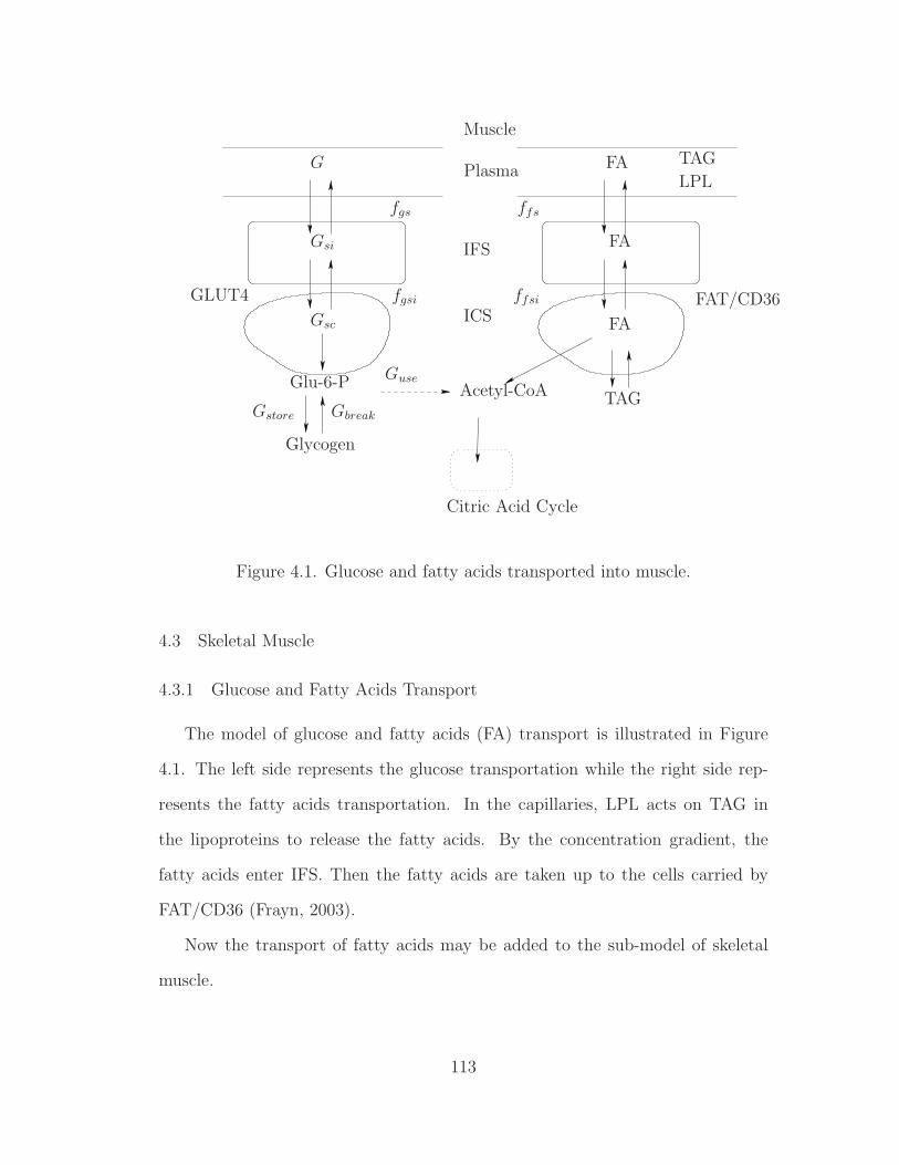
Plasma

IFS

ICS

G

Muscle

fgs

Gsi

Gsc

fgsi

Gstore

GuseGlu-6-P

Gbreak

GLUT4

Glycogen

TAG

TAG

LPL

FA

FA

FA

ffs

ffsi FAT/CD36

Acetyl-CoA

Citric Acid Cycle

Figure 4.1. Glucose and fatty acids transported into muscle.

4.3 Skeletal Muscle

4.3.1 Glucose and Fatty Acids Transport

The model of glucose and fatty acids (FA) transport is illustrated in Figure

4.1. The left side represents the glucose transportation while the right side rep-

resents the fatty acids transportation. In the capillaries, LPL acts on TAG in

the lipoproteins to release the fatty acids. By the concentration gradient, the

fatty acids enter IFS. Then the fatty acids are taken up to the cells carried by

FAT/CD36 (Frayn, 2003).

Now the transport of fatty acids may be added to the sub-model of skeletal

muscle.

113

1. LPL acts on the lipoproteins (CLM and VLDL) in the capillaries which is

slightly suppressed by insulin (Frayn, 2003). Plus, exercise may stimulate

its activity (Frayn, 2003). The rate may also be saturated while increasing

the concentrations of CLM and V LDL.

2. The fatty acids are transported between plasma and IFS via concentration

gradient and taken up into cells by carriers involving FAT/CD36 (Frayn,

2003).

As illustrated in Figure 4.1, fatty acids may be stored as TAG or be converted

into Acetyl-CoA (ACA) after entering the cells. TAG in skeletal muscle is mainly

for local use. It should be noted that ACA is another important metabolite

connecting the glucose metabolism and the fat metabolism as in the Citric Acid

Cycle (also called TCA cycle).

4.3.2 Glucose and Fatty Acid Metabolism

The intracellular metabolism model of skeletal muscle incorporates more in-

formation concerning the fatty acid metabolism. Intracellularly, G6P may be

converted to pyruvate (Pyr) during glycolysis given by the relation:

1 G6P → 2 Pyr. (4.1)

Afterward, pyruvate may be converted to Acetyl-CoA (ACA) and enter the TCA

cycle in the pathway of aerobic respiration. Also, pyruvate is converted to lactate

(Lac) in the pathway of anaerobic respiration as illustrated in Figure 4.2. The

114

relations are expressed as

1 Pyr → 1 ACA (4.2)

1 Pyr → 1 Lac. (4.3)

In skeletal muscle, fatty acids cannot be generated from ACA due to the lack of

fatty acid synthase. But ACA here can result in an inhibition on the oxidation of

fatty acids because ACA may be converted to malonyl-CoA which may suppress

the β-oxidation of fatty acids (Frayn, 2003).

1. The dynamics of Acetyl-CoA (ACA) is determined by the aerobic respi-

ration, pyruvate and fatty acids. Therefore its activity is related oxygen

consumption rate, the cardiac output and the blood flow distribution. The

rate of fatty acids converted into Acetyl-CoA through β-oxidation is inhib-

ited by insulin. The generation of ATP is represented by

1FADH2 → 1.5ATP (4.4)

1NADH → 2.5ATP (4.5)

1Acetyl− CoA → TCA. (4.6)

One of the most common fatty acids is palmitic acid. It is even-number

chained with 2n, n = 8. Two extra units of ATP are consumed to activate

the oxidation (Frayn, 2003). Hence,

ATPproduction = (8− 1)× (1.5 + 2.5) = 28 (4.7)

ATPconsumption = 2. (4.8)

115

− −−

−

−

Gsc Rate1

[ATP]1

1

[GLY]

[G6P]

LactateWork

VO2 KO2s142932

16

2

Insulin

Insulin

InsulinInsulin

Insulin

Insulin

2

12

[Pyr]

11

[ACA]

115

3

Dwn

Syn 1

1

TCA cycle

FA

[TAG]

3 13

4

1

2

28

Figure 4.2. Glucose and fatty acid metabolism in skeletal muscle.

116

2. The dynamics of TAG may be esterified from fatty acids and release fatty

acids for energy requirement. Insulin inhibits the conversion from TAG to

fatty acids and stimulates the esterification of TAG from fatty acids (Frayn,

2003).

3. The dynamics of pyruvate is determined by its relations to G6P, ACA and

lactate. Pyruvate may be generated from lactate through the process of

gluconeogenesis; while pyruvate will produce lactate through anaerobic gly-

colysis (Frayn, 2003).

Therefore, the energy balance between demand and production is influenced by

the concentrations of G6P, Pyr, ACA and lactate.

4.4 The Liver


The transport of glucose and fatty acids in the liver is illustrated in Figure 4.3.

Compared with that in the skeletal muscle, the liver does not have the lipoprotein

lipase (LPL) to utilize lipoprotein particles in the capillaries. Also, VLDL particles

may be released to the circulation system by the liver. Additionally, inside the

liver cells, there exists ketogenesis to release ketone bodies, which may be a fuel

source for the heart, the brain, etc. (Frayn, 2003)

The transport of fatty acids are similar with that in skeletal muscle.

1. The VLDL particles may be released into the plasma. It is secreted by the

liver and contains triacylglycerol, cholesteryl ester and apolipoproteins (Frayn,

2003).

117

Glycogen

GLUT2

Plasma

Liver

IFS

ICS

G

fgl

Gli

Glc

fgli

Gstore

GuseGlu-6-P

Gbreak

ffl

ffli

Acetyl-CoA

Citric Acid CycleKetogenesis

FA

FA

FA

TAG

FAT/CD36

VLDL

Figure 4.3. Glucose and fatty acids transport in the liver.


gradient and taken up into cells by carriers involving FAT/CD36 which is

influenced by the oxygen consumption rate (Frayn, 2003).


Similar with the intracellular glucose and fatty acid metabolism in skeletal

muscle, more details are incorporated into the model of intracellular metabolism

in the liver, such as pyruvate (Pyr), Acetyl-CoA (ACA), fatty acids (FA), etc. For

fatty acid metabolism, there exists the fatty acid synthase in the liver. Hence,

ACA may be converted to fatty acids. And ketone bodies (another form of fuel

mainly used by the heart and the brain) may be produced in the liver through

ketogenesis (Frayn, 2003). These are illustrated in Figure 4.4.

118

−

− −−−Interstitial

Fluid

Interstitial

Fluid

Intracellular

IntracellularGlucose

Lactate

Glucokinase

Rate1

G6-Phosphatase

Rate2

1

Syn

Dwn

1

1

[G6P]

[GLY]

Insulin

Insulin

Insulin

Insulin

Insulin

2

12

1

1

1

4 14

3 13

[TAG]

FA

Kgn

[ACA]

[Pyr]

TCA cycle

VLDL

VO2KO2l

142932

115

[ATP]

16

1 23

2

28

Figure 4.4. Glucose and fatty acid metabolism in the liver.

119

1. The concentration of Acetyl-CoA (ACA) is connected to the aerobic respi-

ration, pyruvate and fatty acids. Therefore it is influenced by the oxygen

consumption rate, the cardiac output and the blood distribution to the liver.

The rate of converting Pyr into ACA is stimulated by insulin (Frayn, 2003).

2. Fatty acids may be broken down to generate ACA through β-oxidation as

a source of TCA cycle while fatty acids may be produced from ACA in

the process of de novo lipogenesis (Frayn, 2003). One of the productions of

β-oxidation is ketone bodies which is another form of fuels (Frayn, 2003).

3. The process of breaking down TAG to fatty acids is inhibited by insulin

while the counter process of esterifying fatty acids to TAG is stimulated by

insulin (Frayn, 2003).

4. The liver may release lipoprotein particles in the form of VLDL to the

plasma (Frayn, 2003).

5. Besides G6P and ACA, the dynamics of pyruvate is also influenced by lactate

through the process of gluconeogenesis and anaerobic glycolysis.

4.5 Adipose Tissue


The transport of fatty acids in the adipose is illustrated in Figure 4.5. The

lipoprotein lipase (LPL) may release fatty acids from lipoprotein particles in the

capillaries.


gradient and taken up into cells by carriers involving FAT/CD36 which is

120

Adipose

Plasma

IFS

ICS

G

fga

Gai

Gac

fgai

Glu-6-P

GLUT4

FA

FA

FA

LPL

ffa

ffai FAT/CD36

TAG

TAGAcetyl-CoA

Figure 4.5. Glucose and fatty acids transported into the adipose.

influenced by the oxygen consumption rate (Frayn, 2003). The lipoprotein

lipase (LPL) is also located at the adipose, which may release fatty acids from

lipoprotein particles in the capillaries, such as CLM and VLDL particles.

2. The glucose transport between the IFS and the ICS is facilitated by glucose

transporter type 4 (GLUT4), which follows the Michaelis-Menten move-

ment (Frayn, 2003).


The intracellular glucose and fatty acid metabolism in the adipose tissue is

illustrated in Figure 4.6.

1. Glucose is carried by GLUT4 into the adipocytes. It may be converted

121

Interstitial

Fluid

Interstitial

Fluid

Intracellular

Space

Intracellular

Space

Gsc

Insulin

Insulin

Insulin

FA

[TAG]

313

Figure 4.6. Glucose and fatty acid metabolism in the adipose tissue.

to fatty acids through the process of lipogenesis which is stimulated by

insulin (Frayn, 2003).

2. The process of breaking down TAG to fatty acids is inhibited by insulin while

fatty acids may be esterified to TAG which is stimulated by insulin (Frayn,

2003).

122

BIBLIOGRAPHY

A. Adrover et al. Physica D, 213:121–146, 2006.

S. Aiston et al. Diabetes, 52(6):1333–1339, 2003.

American Diabetes Association. http://www.diabetes.org/, 2007.

R. Armstrong et al. J. Appl. Physiol., 62:1285–1298, 1987.

S. Ashcroft et al. Biochem J., 174:517–526, 1978.

K. Aukland and R. Reed. Physio. Reviews, 73:1–78, 1993.

A. Avogaro et al. Diabetes, 38:1048–1055, 1989.

A. Bagust and S. Beale. Q J Med., 96:281–288, 2003.

L. V. Basso and R. J. HaveL. J. Clin. Invest., 49:537–547, 1970.

R. Bergman et al. J. Clin. Invest., 68:1456–1467, 1981.

T. Binzoni et al. J. Nucl. Med., 27:192–197, 1998.

P. Bjorntorp et al. Arteriosclerosis, 10:493–496, 1990.

G. Blomqvist et al. European Journal of Nuclear Medicine and Molecular Imaging,

18(10):834–837, 1991.

G. Boden and X. Chen. J. Clin. Invest., 96:1261–1268, 1995.

123

G. Boden et al. J. Clin. Invest., 88:960–966, 1991.

G. A. Brooks. Comparative Biochem. and Physio., 120:89–107, 1998.

M. E. Cabrera et al. Annals of Biomedical Engineering, 26:1–27, 1998.

J. Cadefau et al. Biochem. J., 322(3):745–750, 1997.

D. U. Campos-Delgado et al. ABBI, 2(2):61–71, 2005.

D. U. Campos-Delgado et al. IEEE Transactions on Biomedical Engineering, 53

(11):2201–2210, 2006.

M. L. Cardenas. Glucokinase: Its regulation and role in liver metabolism. Springer-

Verlag, 1995.

A. Caumo and C. Cobelli. Am. J. Physiol., 264:E829–E841, 1993.

J. M. Chan et al. J. Clin. Endocrinol. Metab., 17(9):961–969, 1994.

J. Chase et al. Medical Engineering & Physics, 27:1–11, 2005.

F. Chee et al. IEEE Transctions on Biomedial Engineering, 52(10):1625–1631,

2005.

C. Cobelli et al. Am. J. Physiol. Endocrinol. Metab., 293:E1–15, 2007.

C. Cobelli et al. Mathematical Biosciences, 58:27–60, 1982.

S. R. Colberg et al. J. Clin. Invest., 95:1846–1853, 1995.

F. Creta et al. J. Phys. Chem. A, 110:13447–13462, 2006.

R. Dash et al. BioMedical Engineering OnLine, 6(1):14, 2007.

124

W. C. Duckworth et al. Endocrine Rev., 19:608–624, 1998.

P. Dunn. Measurement and data analysis for engineering and science. Boston:

McGraw-Hill Higher Education, 2005.

D. T. Finegood and B. G. Topp. Diabetes, Obesity and Metabolism, 3(Suppl. 1):

S20–S27, 2001.

K. N. Frayn. Metabolic regulation: a human perspective. Blackwell Publishing,

2003.

T. Fujimoto et al. Med. Sci. Sports Exerc., 35:777–783, 2003.

Y. Fujita et al. Diabetes, 24:17–27, 1975.

M. Giona et al. J. Phys. Chem. A, 110:13463–13474, 2006.

R. Govers et al. Ame. J. Physiol. Endocrinol Metab., 281:E72–80, 2001.

D. Gray. Transplantation proceedings, 17(1):381–382, 1985.

A. Green and E. A. Newsholme. Biochem. J., 180:365–370, 1979.

F. C. Greenwood et al. J. Clin. Invest., 45(4):429–436, 1966.

M. Gregoriou et al. Eur. J. Biochem., 161:171–176, 1986.

J. Grimsby et al. Science, 301(5631):370–373, 2003.

L. C. Groop et al. J. Clin. Invest., 84:205–213, 1989.

L. C. Groop et al. J. Clin. Invest., 87:83–89, 1991.

M.-T. Guillam et al. Proc. Natl. Acad. Sci. USA, 95:12317–12321, 1998.

125

J. Guyton et al. Diabetes, 27:1027–1042, 1978.

D. Harrison et al. Diabetologia, 28:99–103, 1985.

L. C. Harrison et al. J. Clin. Invest., 58:1435–1441, 1976.

T. Hayashi et al. Am. J. Physiol. Endocrinol. Metab., 273(36):E1039–1051, 1997.

J. He et al. Computational Optimization and Application, 23:5–25, 2002.

J. Henriksen et al. J. Clin. Invest., 94:1196–1204, 1994.

P. Hespel and E. Richter. Biochem. J., 284:777–780, 1992.

J. Holloszy et al. Diabetes Metab. Rev., 1:409–424, 1986.

C. J. Homko et al. Diabetes, 52:487–491, 2003.

J. F. Horowitz et al. Am. J. Physiol., 276:E278–E284, 1999.

R. Hovorka et al. Am. J. Physiol. Endocrinol. Metab., 282:E992–1007, 2002.

R. Hume et al. J. Perinatology, 20(5):301–306, 2000.

I. Janssen et al. J. of Appl. Physiol., 89(1):81–88, 2000.

M. D. Jensen et al. J. Clin. Invest., 83:1168–1173, 1989.

R. Johnson et al. Cardiovascular Response to Exercise, chapter Effects of high

altitude and training on oxygen transport and exercise performance, pages 223–

252. Futura Publishing Company, Inc. NY, 1994.

D. Jones et al. J. of Optimization Theory and Application, 79(1):157–181, 1993.

A. Katz et al. Am. J. Physiol. Endocrinol. Metab., 251(1):E65–70, 1986.

126

D. E. Kelley and L. J. Mandarino. J. Clin. Invest., 86:1999–2007, 1990.

P. King et al. Am. J. Physiol. Cell Physiol.., 257:C1128–1134, 1989.

A. H. Kissebah et al. J. Clin. Endocrinol. Metab., 54:254–260, 1982.

L. Kjems et al. Diabetologia, 44:1339–1348, 2001.

S. Klein. J. Clin. Invest., 113(11):1530–1532, 2004.

Y. T. Kruszynska et al. DIABETES, 47:1107–1113, 1998.

D. Levitt. BMC Clinical Pharmacology, 3:3, 2003.

D. Lv and B. Goodwine. Pancreas modeling from ivgtt data using a deterministic

optimal search method. In 2009 IEEE International Conference on Bioinfor-

matics and Biomedicine, pages 303–308, 2009.

L. Mandarino et al. J. Clin. Invest., 80(3):655–663, 1987.

J. Mellor. Biochemistry. Nabu Press, 2010.

S. Nielsen et al. J. Clin. Invest., 113(11):1582–1588, 2004.

C. Owens et al. IEEE Transactions on Biomedical Engineering, 53(6):996–1005,

2006.

G. Pacini and R. Bergman. Computer Methods and Programs in Biomedicine, 23:

113–122, 1986.

G. Pacini et al. Am. J. Physiol., 274:E592–E599, 1998.

M. J. Pagliassotti et al. The role of the liver in maintaining glucose homeostasis.

R.G. Landes Company, 1994.

127

S. Panunzi et al. Theoretical Biology and Medical Modelling, 43:35, 2007.

R. S. Park et al. IEEE Transactions on Biomedical Engineering, 46(2):148–157,

1999.

R. Parker et al. IEEE Engineering in Medicine and Biology, pages 65–73, 2001.

R. S. Parker et al. AIChE Journal, 46(12):2537–2549, 2000.

R. E. Petrosyan. Developments of the intrinsic low dimensional manifold method

and application of the method to a model of the glucose regulatory system.

Master’s thesis, University of Notre Dame, 2003.

R. Printz et al. J. Biol. Chem, 268(7):5209–5219, 1993.

D. Qian and J. T. Brosnan. Biochem J., 313:479–486, 1996.

G. Quiroz and R. Femat. Mathematical Biosciences, 210:554–575, 2007.

J. P. Robertson et al. Biochem. J., 206:577–586, 1982.

M. Roden et al. J. Clin. Invest., 97(12):2859–2865, 1996.

P. Rorsman and E. Renstrom. Diabetologia, 46:1029–1045, 2003.

E. Ruiz-Velazquez et al. Control Engineering Practice, 12:1179–1195, 2004.

V. Sarabia et al. J. Clin. Invest., 90:1386–1395, 1992.

E. V. Schaftingen and I. Gerint. Biochem. J., 362:513–532, 2002.

F. Schuit et al. Proc. Natl. Acad. Sci. USA, 85:3865–3869, 1988.

J. Seoane et al. J. Biol. Chem., 271(39):23756–23760, 1996.

128

S. Shadid et al. Diabetes, 56:1369–1375, 2007.

R. S. Sherwin et al. J. Clin. Invest., 53:1481–1492, 1974.

L. S. Sidossis et al. J. Clin. Invest., 98(10):2244–2250, 1996.

J. T. Sorensen. A Physiologic Model of Glucose Metabolism in Man and its Use to

Design and Assess Improved Insulin Therapies for Diabetes. PhD thesis, MIT,

1985.

E. Sternlicht et al. Am. J. Physiol. Endocrinol. Metab., 256:E227–230, 1989.

L. Stryer. Biochemistry. New York: W.H. Freeman and Company, 5th edition,

2002.

D. Swain. Old Dominion University’s Quest, 3(2):9–11, 2000.

N. Syed and R. Khandelwal. Molecular and Cellular Biiochemistry, 211(1-2):

123–136, 2000.

B. Thorsteinsson. Danish Medical Bulletin, 37(2):143–153, 1990.

I. M. Tolic et al. J. Theor. Biol., 207:361–375, 2000.

B. Topp et al. J. Theor. Biol., 206:605–619, 2000.

O. Vahidi et al. Development of a physiological model for patients with type 2

diabetes mellitus. In American Control Conference, 2010.

P. Vicini et al. Am. J. Physiol., 273:1024–1032, 1997.

C. Villar-Palasi. Biochim Biophys Acta., 1095(3):261–267, 1991.

C. Villar-Palası and J. J. Guinovart. FASEB J., 11:544–558, 1997.

129

R. Weiss et al. Diabetes, 54:1735–1743, 2005.

G. Wilcox. Clin. Biochem., 26:19–39, 2005.

H. Yki-Jarvinen et al. J. of Clin. Invest., 79:1713–1719, 1987.

B. Zinker et al. Diabetes, 42:956–965, 1993.

This document was prepared & typeset with LATEX2ε, and formatted withnddiss2ε classfile (v3.0[2005/07/27]) provided by Sameer Vijay.

130

Documents

CONSTRUCTION, ANALYSIS AND VALIDATION OF A …controls.ame.nd.edu/~bill/students/dayu.pdf · CONSTRUCTION, ANALYSIS AND VALIDATION OF ... Nightingale and Alice Nightingale for all