Constructing Inverse Probability Weights for Selection Bias Constructing Inverse Probability Weights for Static Interventions

Kunjal Patel, DSc MPHSenior Research ScientistHarvard T.H. Chan School of Public Health

Acknowledgement

Slides contributed by Miguel Hernán, Ellie Caniglia, or adapted from Causal Inference (Chapman & Hall/CRC, 2017) by Miguel Hernán and Jamie Robins Any mistakes are my own

Chapters of book and SAS, STATA, and R code freely available at http://www.hsph.harvard.edu/miguel-hernan/causal-inference-book/

You can “like” Causal Inference at https://www.facebook.com/causalinference

Summary of day 1

Well-defined intervention

Static vs. dynamic interventions

Definition of an average causal effect

Why is randomization important?

Conditional exchangeability assumption to identify a causal effect

When standard adjustment methods fail

IP weights for treatment

Formulation of a well-defined study question

Well-defined causal inference questions can be mapped into a target trial

Specify the protocol of the target trial including: Eligibility criteria Treatment strategies Randomized treatment assignment Follow-up period Outcome Causal contrast of interest Analysis Plan

Hernan, Robins Am J Epidemiol. 2016;183(8):758–764

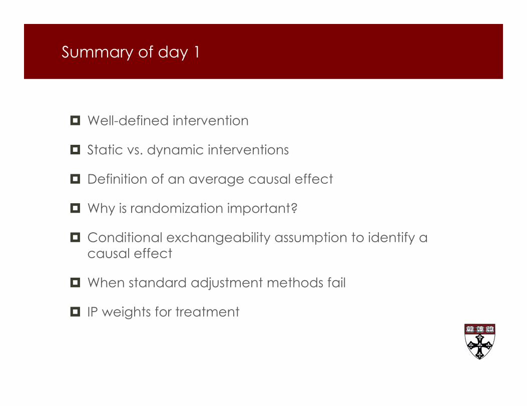
Classification of sustained treatment strategies

Static a fixed strategy for everyone Example: treat with 150mg of daily aspirin during 5

years Case example: initiate HAART

Dynamic a strategy that assigns different values to different

individuals as a function of their evolving characteristics

Example: start aspirin treatment if coronary heart disease, stop if stroke

Case example: initiate HAART if CD4 drops below 500 cells/mm3

Definition of an average causal effect

l

Each person has two counterfactual outcomes: Outcome Y if treated - Yi, a=1

Outcome Y if untreated – Yi, a=0

Individual causal effect: Yi, a=1 ≠ Yi, a=0

Cannot be determined except under extremely strong assumptions

Average (population) causal effect: E[Ya=1 = 1] ≠ E[Ya=0 = 1] Can be estimated under:

No assumptions (ideal randomized experiments) Strong assumptions (observational studies)

Why is randomization important?

When group membership is randomly assigned, risks are the same

Both groups are comparable or exchangeable

Exchangeability is the consequence of randomization

Within levels of the covariates, L, exposed subjects would have had the same risk as unexposed subjects had they been unexposed, and vice versa

Counterfactual risk is the same in the exposed and the unexposed with the same level of L

Pr[Ya=1|A=1, L=l] = Pr[Ya=1|A=0, L=l] A Ya|L=lYa A|L=l

Equivalent to randomization within levels of L

Implies no unmeasured (residual) confounding within levels of the measured covariates L

Conditional exchangeability

Methods to compute causal effects

Stratification

Regression

Matching

Standardization

Inverse probability weighting

ALL assuming conditional exchangeability

Choice of method depends on type of strategies

Comparison of strategies involving point interventions only All methods work if all baseline confounders are measured

Comparison of sustained strategies Generally only causal inference methods work Time-varying treatments imply time-varying

confounders possible treatment-confounder feedback

Conventional methods may introduce bias even when sufficient data are available on time-varying treatments and time-varying confounders

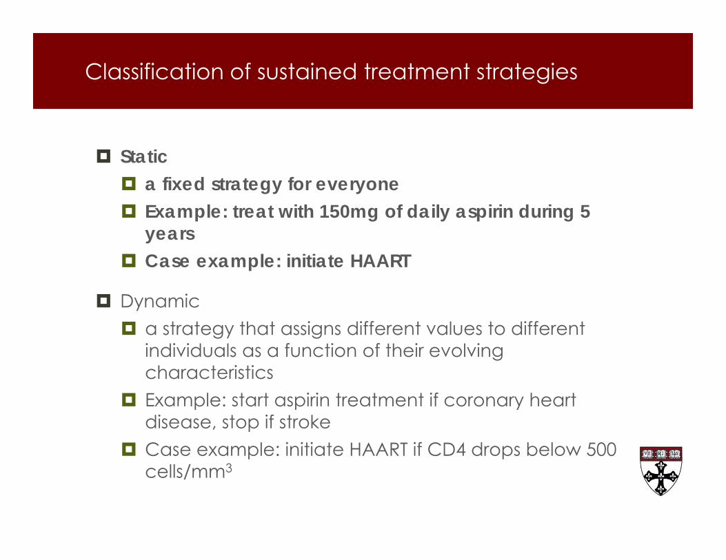
Problem with stratified analytic approach

L0 A0 L1 A1 Y1

U

Interested in the cumulative effect of treatment. L1 is a confounder for the treatment A1 – if don’t adjust for it then treatment effect is confounded. Also could induce selection bias (collider). L1 is affected by A0 – if adjust for L1 then losing some of the effect of A0.

Stabilized inverse probability of treatment weights

Numerator: The probability that the subject received his/her observed treatment at week k, conditional on past treatment history and baseline covariates.

Denominator: The probability that the subject received his/her own observed treatment at week k, given past treatment history and covariate history (baseline and time-dependent).

Directed Acyclic Graph in pseudopopulation with SW

V A0 L1 A1 Y

U

Estimating IPW and fitting the MSM

Estimate SW for both treatment and censoring: Fit logistic regression models for treatment and censoring Use predicted values from the models to calculate stabilized

weights

Estimate the IPW estimate of HAART on mortality: Fit weighted pooled logistic model using the estimated

stabilized weights. Use “robust” variance estimators (GEE) to allow for

correlated observations created by weighting –conservative 95% CI.

Case study

Introduction/background

The use of antiretroviral drugs (ARVs) during pregnancy has dramatically decreased the incidence of perinatal transmission of HIV

The effects of in utero exposure to ARVs on neurodevelopment in perinatally HIV-exposed but uninfected (PHEU) infants requires further study

Previous research evaluating developmental outcomes in PHEU infants identified atazanavir as a safety concern

A comparative safety study was needed to confirm these findings

Objective

To evaluate the effect of in utero exposure to ARV regimens containing atazanavir compared to non-atazanavir-containing regimens on neurodevelopment at 9-15 months of age

using observational data from a cohort of PHEU infants

with a comparative safety design

Study population

SMARTT protocol of PHACS

Pregnant women living with HIV enrolled in the dynamic cohort

Not on ARVs at their last antepartum menstrual period Initiated ARVs during pregnancy

Excluded sites in Puerto Rico

Excluded if infant less than 15 months of age by July 1, 2014

Exposure ascertainment

Outcome ascertainment

Bayley Scales of Infant and Toddler Development – Third Edition (Bayley-III) Administered at 9-15 months of age Only available in English Provides 5 scores: Cognitive Language Motor Social-emotional General adaptive

Secondary outcomes

Neonatal outcomes Low birth weight (≤2500 grams) Gestational age Prematurity (gestational age <37 weeks) Neonatal hearing

Head circumference z-scores at 9-18 months

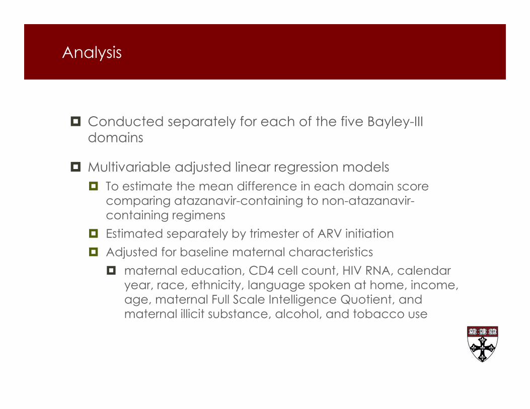
Analysis

Conducted separately for each of the five Bayley-III domains

Multivariable adjusted linear regression models To estimate the mean difference in each domain score

comparing atazanavir-containing to non-atazanavir-containing regimens

Estimated separately by trimester of ARV initiation Adjusted for baseline maternal characteristics

maternal education, CD4 cell count, HIV RNA, calendar year, race, ethnicity, language spoken at home, income, age, maternal Full Scale Intelligence Quotient, and maternal illicit substance, alcohol, and tobacco use

l

Missing outcome data

~40% had incomplete or invalid results for one or more Bayley-III domains

l

Options for analysis

Analyze observed non-missing outcome data Any problems with this approach?

Selection bias

Bias that arises when the parameter of interest in a population differs from the parameter in the subset of individuals from the population that are available for analysis

Selection bias for descriptive measures (e.g., prevalence) because of non-random sampling

Selection bias for effect measures (e.g., causal risk ratio) because of differential loss to follow-up

Selection bias for effect measures

Differential loss to follow-up/censoring

Missing outcome/Non-response

Healthy worker bias

Self-selection/volunteer bias

Structure of selection bias (under the null)

Bias arises as the consequence of conditioning on a common effect of treatment and outcome Or on a common effect of a cause of the treatment and a

cause of the outcome

That is, the design or the analysis is conditioned on “being selected for analysis” C=0

Is bias due to differential loss to follow-up possible in randomized experiments?

Yes?

No?

Aside: Is bias due to self-selection possible in randomized experiments?

Yes?

No?

Aside: Internal vs. external validity in randomized experiments

Internal validity the estimated association has a causal interpretation in the

studied population i.e., no selection bias, no confounding

External validity the estimated association has a causal interpretation in

another population i.e., generalized or transportability

In randomized experiments There is internal validity Perhaps not external validity

Simplified case example

HIV-exposed uninfected infants

Variables: A=1: In utero exposure to ATV L=1: Low maternal CD4 count at delivery C=1: Missing 1-year Bayley exam Y=1: Neurocognitive deficit

Treatment status randomized No confounding

Under the null: No effect of in utero ATV exposure and neurocognitive function

Case example: Directed Acyclic Graph

Where: L: Maternal CD4 count at delivery A: Maternal exposure to ATV C: Censored Y: Neurocognitive deficit in infant at 1 year U: Unmeasured covariate – Maternal underlying immune

function

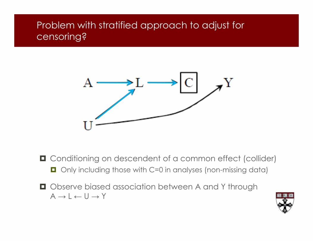
Problem with stratified approach to adjust for censoring?

Conditioning on descendent of a common effect (collider) Only including those with C=0 in analyses (non-missing data)

Observe biased association between A and Y through A → L ← U → Y

Alternative structure of selection bias due to differential loss to follow-up/non-response or missing data

Where: L: Smoking intensity at baseline A: Smoking cessation C: Censored Y: Weight gain U: Lifetime history of smoking

Stratified approach will not cause bias if measure and adjust for L

Approaches for adjustment for selection bias

Stratification

Regression

Inverse probability weighting

Approach depends on the structure of selection bias

Simplified case example original data

Among A=0: No in utero exposure to ATV L=1: Low maternal CD4 count at delivery C=1: Missing 1-year Bayley exam Y=1: Neurocognitive deficit

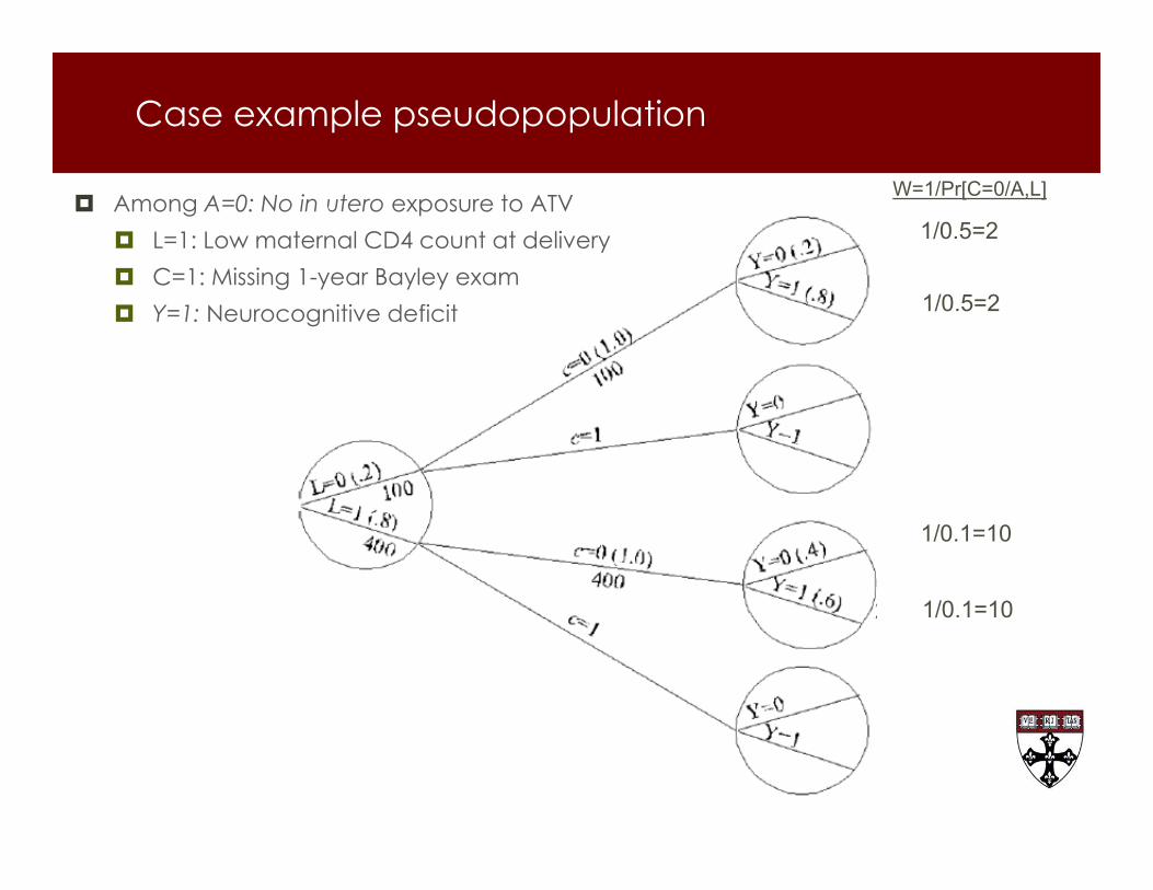
Case example pseudopopulation

Among A=0: No in utero exposure to ATV L=1: Low maternal CD4 count at delivery C=1: Missing 1-year Bayley exam Y=1: Neurocognitive deficit

W=1/Pr[C=0/A,L]

1/0.5=2

1/0.5=2

1/0.1=10

1/0.1=10

Directed Acyclic Graph in pseudopopulation

What is an assumption are we making?

Conditional exchangeability

Average outcome in the uncensored participants is the same as the average outcome in the censored participants with the same values of A and L

Or selection is randomized within levels of A,L

Use of models for IPW

Reality is we deal with high-dimensional data with multiple covariates (Ls), some with multiple levels Cannot obtain meaningful non-parametric estimates of the

weights Model the probability of being uncensored with Ls (and A)

as the covariates

Some individuals may contribute a really high weight due to their a relatively small probability of being uncensored given their exposure and covariate history Stabilize the weights by using the probability of being

uncensored given treatment and baseline covariates in the numerator

Apply stabilized weights (SW) to estimate the parameters of a marginal structural model reduce variance in model for the outcome

Stabilized inverse probability of censoring weights

Numerator: The probability that the subject was uncensored at week k, conditional on past treatment history and baseline covariates.

Denominator: The probability that the subject was uncensored at week k, given past treatment history and covariate history (baseline and time-dependent).

Pr {C(k)=0/Ᾱ(k),V}

Pr {C(k)=0/Ᾱ(k), L(k)}

Estimating IPW and fitting the MSM

Estimate SW for censoring: Fit logistic regression models for being uncensored Use predicted values from the models to calculate stabilized

weights

Estimate the IPW estimate of in utero ATV exposure on neurocognitive scores at 1-year: Fit weighted linear regression models using the estimated

stabilized weights. Use “robust” variance estimators (GEE) to allow for

correlated observations created by weighting –conservative 95% CI.

Summary: IP weights

To adjust for confounding Use IP weights for treatment – IPTW

To adjust for selection bias Use IP weights for censoring – IPCW

To adjust for both biases Multiply IPTW x IPCW

Case Example: Predictors of Censoring

Baseline covariates: maternal education, CD4 cell count, HIV RNA, calendar year, race, ethnicity, language spoken at home, income, age, maternal Full Scale Intelligence Quotient, and maternal illicit substance, alcohol, and tobacco use

Post-baseline covariates: mother’s last CD4 in pregnancy, positive test for STI in pregnancy, infant low birth weight, and gestational age at delivery

Primary effect estimates of interest

Effect of in utero ATV exposure during the 1st trimester on the following Bayley scores:

Cognitive Language Motor Social-emotional General adaptive

Effect of in utero ATV exposure during the 2nd/3rd trimester on the following Bayley scores:

Cognitive Language Motor Social-emotional General adaptive

Results

Characteristics of Study Population

Atazanavir-containing regimen(n=167)

Non-atazanavir-containingregimen(n=750)

Results

Characteristics of Study Population

Characteristic Atazanavir-containing regimen

(n=167)

Non-atazanavir-containing regimen

(n=750)ARV initiation

First trimester 55 (33%) 227 (30%)

Second or third trimester

112 (67%) 523 (70%)

Results

Characteristics of Study Population

Characteristic Atazanavir-containing regimen

(n=167)

Non-atazanavir-containing regimen

(n=750)ARV initiation

First trimester 55 (33%) 227 (30%)

Second or third trimester

112 (67%) 523 (70%)

Age older(mean 29 years)

younger(mean 27 years)

Cognitive scores lower(mean 84.3)

higher(mean 86.5)

Initiate ARVs 2011-2014

more likely (40%)

less likely(26%)

Results

Common Regimens

Number of initiators

Type of regimen

Atazanavir-containing regimens

Atazanavir, emtricitabine,tenofovir, ritonavir 126 (75%) Boosted PI with 2 NRTIs

Non-atazanavir-containing regimens

Lopinavir, zidovudine, lamivudine, ritonavir 335 (45%) Boosted PI with 2 NRTIs

Zidovudine, lamivudine, abacavir 134 (18%) 3 NRTIs

Results

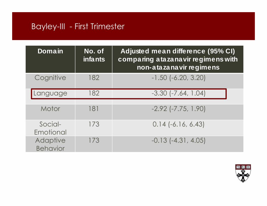
Bayley-III - First Trimester

Domain No. of infants

Adjusted mean difference (95% CI)comparing atazanavir regimens with

non-atazanavir regimensCognitive 182 -1.50 (-6.20, 3.20)

Language 182 -3.30 (-7.64, 1.04)

Motor 181 -2.92 (-7.75, 1.90)

Social-Emotional

173 0.14 (-6.16, 6.43)

Adaptive Behavior

173 -0.13 (-4.31, 4.05)

Results

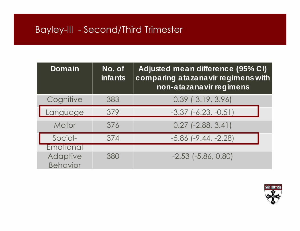
Bayley-III - Second/Third Trimester

Domain No. of infants

Adjusted mean difference (95% CI)comparing atazanavir regimens with

non-atazanavir regimensCognitive 383 0.39 (-3.19, 3.96)Language 379 -3.37 (-6.23, -0.51)

Motor 376 0.27 (-2.88, 3.41)Social-

Emotional374 -5.86 (-9.44, -2.28)

Adaptive Behavior

380 -2.53 (-5.86, 0.80)

Results

Secondary Outcomes

Results

Outcome No. of infants

No. of outcomes

Adjusted mean difference (95% CI)comparing atazanavir regimens with

non-atazanavir regimens

Head circumference

z-score

652 -- -0.45 (-0.66, -0.24)

Gestational age (weeks)

906 --0.00 (-0.35, 0.36)

Adjusted risk ratio (95% CI)Hearing screen

referral898 31 1.21 (0.53, 2.80)

Low birth weight 911 1631.06 (0.73, 1.53)

Prematurity (<37weeks)

911 161 1.00 (0.68, 1.48)

Conclusions

Conclusions (1)

Conclusions

Atazanavir-containing regimens may lower infants’ performance on the Language domain of the Bayley-III by about 3.4 points, regardless of trimester of initiation

Atazanavir-containing regimens may lower infants’ performance on the Social-Emotional domain by 5.9 points, when initiated in the second/third trimester

Conclusions (2)

Conclusions

The lack of an estimated effect of initiation of atazanavirin the first trimester on social-emotional development may be explained by a high proportion of women who switched to another ARV regimen later in pregnancy

Conclusions (3)

Conclusions

Atazanavir could affect neurodevelopment via hyperbilirubinemia

Clinical implications may be small, but future work should evaluate whether the differences observed in this study persist over time

Acknowledgements

under cooperative agreements HD052104 (PHACS Coordinating Center, Tulane University School of Medicine) and HD052102 (PHACS Data and Operations Center, Harvard T. H. Chan School of Public Health).

Ellen Caniglia was supported by T32 AI007433 from NIAID

We thank the study participants, clinical sites, PHACS Community Advisory Board, Frontier Science & Technology Research Foundation, and Westat.

PHACS is funded by:

PHACS US Clinical Sites

Ann & Robert Lurie Children’s Hospital of Chicago

Baylor College of Medicine

Bronx Lebanon Hospital Center

Children's Diagnostic & Treatment Center

Children’s Hospital, Boston

Children’s Hospital of Philadelphia

Jacobi Medical Center

New York University School of Medicine

St. Christopher’s Hospital for Children

St. Jude Children's Research Hospital

San Juan Hospital/Department of Pediatrics

SUNY Downstate Medical Center

SUNY Stony Brook

Tulane University Health Sciences Center

University of Alabama, Birmingham

University of California, San Diego

University of Colorado Health Sciences Center

University of Florida/Jacksonville

University of Illinois, Chicago

University of Maryland, Baltimore

Rutgers- New Jersey Medical School

University of Miami

University of Southern California

University of Puerto Rico Medical Center