Constraints on stretching by paired vortex

structures II. The asymptotic dynamics of

blow-up in three dimensions

Stephen Childress

April 6, 2010

Abstract

This paper continues our study of the use of paired vortex structures inthe construction of incompressible Euler flows in three dimensions whichproduce substantial vorticity growth. These flows, which have been con-sidered before as candidates for Euler blow-up, are here derived in a geom-etry which is the product of moving planar curve C(t), the center vortexline, and locally almost two-dimensional fluid motion in planes P (t) or-thogonal to the curve. In the present part we show that the constructionof a non-self-similar flow of the kind proposed here can be reduced by con-tour averaging to a generalized differential system. Each section consistsof an invariant 2D Euler flow, assumed here to have the contour structureof paired vortices of opposite sign, of a size compatible with the requisitepropagation speed of the singular cocoon. Axial flow within the cocoonalters the local contours from section to section. This leads to a complexinteraction of the generalized differential system with the kinematics ofthe center vortex.

To simplify this interaction we propose here that the Batchelor coupleintroduced in part I is one of a family of invariant 2D flows suitable for theconstruction of a singular Euler flow in 3D. This family includes vortices ofarbitrarily small cross-section, allowing the self-induced stretching of thevortex pair to be decoupled from the variation of the circulation profilesby the axial flows. We thus propose to show in the present paper thatthe thin-vortex limit of these extensions of the Lamb-Chaplygin-Batchelorcouple (acknowledging the prior presentations of this solution of the steadyEuler equations) offers the first clean example of blow-up of Euler flowsin three dimensions.

A crucial issue is the axial flow in the vortices, which we shall treatin this part using a one-dimensional model. This has the advantage ofleading, for the fixed-point problem at the core of the existence of the blow-up, to an ODE problem which is readily solved numerically. Surprisingly,our model shows that the squeezing down of the cross-section of the self-stretching vortices overcomes the axial flow induced by the lower pressuresof the most stretched section, so that the axial flow is in fact away fromthe singularity region.

1

Some implications of such solutions for Euler flow theory are discussed.We conjecture that the solutions are highly unstable and not directlyobservable in numerical simulations. We also give reasons for the absenceof any such singularities for the Navier-Stokes equations. The final phaseof this research will deal with the full PDE problems for the non-self-similar Euler flow associated with the blow-up.

1 Introduction

The present paper continues our study of vortex stretching in flows of simpletopology. In [Childress (2006)], hereafter referred to as I, we argued that Eulerblow-up, if it occurs at all, is in some sense extremely rare. In the present paperwe explore a family of flows which are related to paired vortex flows previouslyproposed as candidates for finite time singularities. Studies of this kind are im-portant even if they lead to negative results, since it is essential to understandthe often invoked “depletion of nonlinearity” as an explanation of the lack ofany convincing evidence of Euler blow-up. However the present work suggeststhat in fact there do exist Euler flows (probably unstable) which produce infi-nite vorticity in finite time. The flows we study involve non-self-similar vortexstretching of paired filaments without the constraint of non-swirling axial sym-metry, obtained in the kinematic model put forward in section 3 of I. We use theterm “kinematic” in a slightly perverse way, referring to the blow-up of pairedvortices as obtained in I, without a dynamical basis for the relation between theadvection of vortices by the normal, and the local Jacobian of the center vortexof the pair.

We first review some of the ideas presented in I. According to [Beale, Kato & Majda (1984)]blowup is accompanied by infinite vorticity, and this is achieved by the stretch-ing of vortex lines. The stretching can be achieved by the variation of thevelocity component tangent to the line (shear stretching), or else by advec-tion in the direction of the negative normal of a curved vortex line (expansivestretching). Shear stretching is important in the model studied by [Pelz (2001)]and may well dominate the stretching events in turbulent flows on many scales.But it involves sheared vortical structure in order to make the velocity inducedby vortex tube A stretch tube B and vice versa. Expansive stretching was in-voked and pioneered in the models of [Siggia (1985), Pumir & Siggia (1990)],and of [Kerr (2005)], and has the attraction of being accessible by vortex lineswhich are locally parallel, provided that paired structures of opposite sign areso aligned. In particular nearly two-dimensional flow structures are capable ofself-stretching. This makes paired vortex structures attractive for analysis ofsingular behavior in Euler flows. Numerically, however, singularity formationseems to be stalled by deformation of the structures in the final phase. Thestructures studied by Kerr are not locally 2D, but are similar in some respectsto the “hairpin” singularities of the kinematic models considered in I. We willdiscuss below the relation of our work to that of [Pumir & Siggia (1990)].

To investigate how fast paired structures can self-stretch, we considered in I

2

the simplest family of Euler flows in 3D where this happens, namely axisymmet-ric flow without swirl, where the vorticity has the form (0, 0, ωθ) in cylindricalpolar coordinates and all vortex lines are circles about a common axis. It is wellknown ([Majda & Bertozzi (2002)]) that ωθ then grows at most like an expo-nential in time, so blow-up does not occur. In I we examined the implications ofconstant vorticity support volume on the maximal rate of growth. We estimatedkinematically the optimal configuration for maximal expansive stretching of atarget ring given an initial bound on |ωθ/r|, and found that vorticity grew infact no faster than O(t2). We called this optimizing arrangement of vorticitya kinematic cocoon. The kinematic cocoon conserves volume, but not kineticenergy, which grows in proportion to the radius of the target ring.

We also found in I that there is another cocoon construction which conservesenergy but not volume, leading to growth as O(t4/3). It appears that bothconstraints can be satisfied kinematically by cocoons which shed filamentaryvorticity, although the constraint of energy conservation is essential only whenaxial symmetry is imposed. This point will be important in the present paper.

The O(t2) maximal growth of the kinematic cocoon of constant volume sug-gests comparison with quasi-2D flows. A classical solution of Euler’s equationsin two dimensions, consisting of a pair of oppositely sign vortical regions con-tained within a circular boundary r = a, may be found in [Batchelor (1967)],a solution that goes back to the work of Lamb and Chaplygin. 1 The dipolarstructure moves without change of form at a constant velocity. In three dimen-sions we may consider an analogous thin toroidal structure as an initial vorticityof an axisymmetric flow without swirl, which then expands while maintaining aself-similar structure. Since vortical flux is conserved, ωθa

2 = O(1). The speedof propagation ∼ ωθa, and the torus volume must be conserved, Ra2 = O(1)where R is the large radius of the torus. It follows the speed at large R is ∼

√R,

leading to R = O(t2), at a rate satisfying our bound. This estimate omits thefact already noted, that the kinetic energy of the toroidal structure, which mayestimated as O(ω2

0a4R) ∼ O(R) increases, so the circular boundary of the vor-

tex does not survive–there must be core deformation to conserve energy, alongwith a lessening of vortex stretching.

If one relaxes the constraint of axial symmetry and assumes that pairedstructure moves as a Lamb-Chaplygin-Batchelor (LCB) couple in all local sec-tions, then, as we showed in I, of a line moving in this way by the normalproduces a finite time singularity. At the singular time vorticity is infinite at apoint, but only a finite amount of total stretching of vortex lines has occurred.The question raised in the present part is essentially, can this kinematic pic-ture survive if the paired structure satisfies Euler’s equations in an appropriatesense associated with the asymptotics of the singularity? The dynamics involvespossible core deformation as well as the creation of axial flows induced by thepressure gradients developed when a vortex is stretched locally. We shall show

1In I we termed this structure a Batchelor couple, because it was a prominent examplein [Batchelor (1967)]. As might be expected, the solution has a richer history, which wasdiscussed in [Meleshko & van Heijst (1994)]. Horace Lamb and S.A. Chaplygin describe thisstructure and its variants over a century ago, see [Lamb (1906), Chaplygin (1903)]

3

that if the paired structure is initially a LCB couple at each section, it will sub-sequently evolve according to a generalized differential system. The dynamicsmust, under this system, depart from the kinematics described in I.

Nevertheless, the dynamical description developed here contains the possibil-ity of using other 2D Euler solutions as the underlying cross-sectional flow, andwe argue here that there exists a family of flows including the Lamb-Chaplygin-Batchelor flow. Included are paired vortex tubes of near circular vortex section,which allow the implications of the generalized system to be studied analytically.This is a key step which breaks the deadlock over coupling of the velocity of thevortex pair with the core dynamics. The two essential features are, first, thefact that it is only the total circulations of the vortices, the constants ±Γ say,which determine the velocity of the pair, and second, for small cores the coreboundary is essentially a circle, allowing an axisymmetric treatment in classicalterms,

2 The dynamic cocoon

We now refer to curve C(t), studied in section 3 of I, with γ ∈ (1/2, 1), as thecenter vortex. It will actually be a vortex line on which vorticity vanishes. Weintroduce the time-dependent orthogonal curvilinear coordinate system derivedfrom the center vortex, with triad (n,b, t), coordinates (ξ, η, ζ), and metricds2 = dξ2 + dη2 + h2dζ2, where h = 1 − ξκ. The cocoon boundary will bethe surface C : ξ2 + η2 = 1

4κ−2,−∞ < ζ < +∞, the numerical factor insuring

that h remains positive within the cocoon. We wish to solve Euler’s equationswithin the cocoon starting at an initial time t = T < 0, and to do so we needto supply an initial vorticity field, then track its evolution under the constraintof Euler’s equations and some boundary conditions associated with the cocoonboundary. We assume that the fluid density is unity. As we shall make clearpresently, the initial vorticity will be confined within another surface B : ξ2 +η2 = r2B(ζ),−∞ < ζ < +∞, and we may in fact choose max−∞<ζ<+∞ κrB tobe as small as we like. Indeed on the curve g is positive and has the estimate(??) for sigma large, from which it follows that κ/g is bounded as a functionof σ. Thus we may, in the LCB couple, fix a to match the curve velocity, thedecrease it everywhere by a constant multiplier while simultaneously increasingthe flux K by the inverse factor.

For t > T the surface B will be material and track the motion of the centercurve C with β = 2 . The tube bounded by B will thus be stretched and thetransverse ξ, η dimensions contract, so that as we can understand its evolutionfrom the dynamics of C. Therefore, the crucial issue is the behavior of thecurve in the neighborhood of B as τ → 0 with σ fixed. Assuming that we haveindeed set up the initial vorticity so as to track the motion of C. Then, ouranalysis shows that ξ, η ∼ O(τγ) and κ−1 ∼ ζ ∼ O(τ1−γ) where A ∼ B meansthat A is neither much small than, nor much larger than B as τ → 0. We willwee that vorticity kinematics will then imply that u ∼ v ∼ O(τ−γ), and it willalso transpire that w ∼ O(τ−γ) and that pressure satisfies p ∼ O(τ−2γ). These

4

estimate allow us to estimate the size of all terms in Euler’s equations in thiscoordinate system.

In Cartesian coordinates Euler’s equations for an incompressible fluid are(assuming that the fluid density is unity)

ut + u · ∇u + ∇p = 0, ∇ · u = 0. (1)

To write these equations in the new coordinate system we need a few differ-entiation formulas derived using the chain rule. For any scalar function f wehave

∂f

∂t

∣

∣

∣

ξ,η,ζ0=∂f

∂t

∣

∣

∣

x,y,z+∂x

∂t

∣

∣

∣

ξ,η,ζ0· ∇f. (2)

We assume that the curve moves according in the direction of the normal as inI, but now take the curve velocity as u = U(ζ, t) in the direction of the normal ,since we want to use u, v, w for fluid velocity in the present coordinate system.

Thus ∂x∂t

∣

∣

∣

ξ,η,ζ0= Un. Then

∂f

∂t

∣

∣

∣

x,y,z=∂f

∂t

∣

∣

∣

ξ,η,ζ0− U

∂f

∂ξ. (3)

We also have

∂(n,b, t)

∂t

∣

∣

∣

x,y,z=∂(n,b, t)

∂t

∣

∣

∣

ξ,η,ζ0+ U

∂(n,b, t)

∂ξ=∂(n,b, t)

∂t

∣

∣

∣

ξ,η,ζ0, (4)

so that, since∂(n,b, t)

∂t

∣

∣

∣

ξ,η,ζ0= (Uζt, 0,−Uζn), (5)

we have

∂(un + vb + wt)

∂t

∣

∣

∣

ξ,η,ζ0= n(Du+wUζ) + bDv + t(Dw − uUζ), (6)

where

D =∂

∂t

∣

∣

∣

ξ,η,ζ0− U

∂

∂ξ. (7)

We also have the standard formulas

u · ∇u =[

uuξ + vuη + h−1wuζ − h−1w2hξ

]

n

+[

uvξ + vvη + h−1wvζ − h−1w2hη

]

b

+[

uwξ + vwη + h−1wwζ + h−1w(uhξ + vhη)]

t. (8)

The equation ∇ · u = 0 becomes

∂hu

∂ξ+∂hv

∂η+∂w

∂ζ= 0 (9)

5

Finally, the pressure term is ∇p = (pξ, pη, h−1pζ). Taking the density of the

fluid to be unity, and setting u = U + u′, the equations of motion become

u′t0 + u′u′ξ + vu′η + (1 + h−1)wu′ζ − h−1w2hξ + pξ + Ut = 0, (10)

vt0 + u′vξ + vvη + h−1wvζ − h−1w2hη + pη = 0, (11)

wt0−u′Uζ+u′wξ+vwη+h−1wwζ+h−1w(uhξ+vhη)+h−1pζ−UUζ = 0, (12)

∂hu′

∂ξ+∂hv

∂η+∂w

∂ζ+ Uhξ = 0 (13)

Here the subscript t0 indicates that ζ0, not ζ, is held fixed.Since hη = 0, hξ = −κ, the equations for ω ≡ vξ − uη and w are

ωt0 + u′ωξ + vωη + h−1wωζ + h−1ω(u′κ+ Uκ−wζ) − 2h−1wwηκ

−(1 + h−1)wηUζ + h−2κwvζ + h−1wξvζ − h−1wηu′

ζ = 0, (14)

wt0 − u′Uζ + u′wξ + vwη + h−1wwζ − h−1wuκ+ h−1pζ − UUζ = 0. (15)

We rearrange these equations as follows:

u′ωξ + vωη = Fω, (16)

u′wξ + vwη = Fw, (17)

u′ξ + vη = G. (18)

Here

Fω = −ωt0 − h−1wωζ − h−1ω(u′κ− wζ) − h−1ωUκ+ 2h−1wwηκ

+(1 + h−1)wηUζ − h−2κwvζ − h−1wξvζ + h−1wηu′

ζ, (19)

Fw = −wt0 + Uκw − h−1wwζ + h−1wUκ+ h−1wu′κ− h−1pζ + UUζ , (20)

G =1

hUκ− 1

hwζ +

1

hκu′. (21)

2.1 Ordering and expansion

We now consider the ordering of terms in the singular region σ = O(1) as τ → 0.We have the underlying orders

(ξ, η, ζ) = O(τγ , τγ , τ1−γ), (u′, U, v, w) = O(τ−γ , τ−γ, τ−γ , τ−γ), (22)

and alsoω = O(τ−2γ), κ = O(τγ−1). (23)

Note that we have assumed the axial flow component w is of the order of thetransverse components although no formal order is indicated by the motion of

6

C. We also have h = 1 +O(τ2γ−1), t = O(τ ), p = O(τ−2γ), and recall γ > 1/2.We may therefore rewrite (16),(17),(18) as follows:

u′ωξ + vωη = F (1)ω + O(τ−2), (24)

u′wξ + vwη = F (1)w +O(τγ−2), (25)

u′ξ + vη = G(1) + O(τ2γ−2). (26)

HereF (1)ω = −ωt0 − Uκω −wωζ − ω(u′κ− wζ) + 2wwηκ

+2wηUζ −wξvζ + wηu′

ζ = O(τ−2γ−1), (27)

F (1)w = −wt0 + Uκw + u′Uζ −wwζ + wu′κ− pζ + UUζ = O(τ−γ−1), (28)

G(1) = Uκ−wζ + κu′ = O(τ−1). (29)

The orders of these forcing functions reflect the order of every term in thefunction.The left-hand sides of (24),(25),(26) are respectively τ−4γ , τ−3γ, τ−2γ,so that in each equation the ratio of forcing to left-hand side is O(τ2γ−1) = o(1),and the ratio of the error to the left-hand side is O(τ4γ−2). Thus if δ is take asO(τ2γ−1), we may introduce expansions of the form

q = q0 + q1 + . . . , qn = (u′n, vn), w = w0 +w1 + . . . , (30)

ω = ω0 + ω1 + . . . , p = p0 + p1 + . . . , (31)

where the subscript 1 terms are smaller than the subscript 0 terms by a factorof δ, and the errors are still smaller by another factor δ.

2.2 The first-order solution and compatibility of the zeroth-

order solution

The first-order terms satisfy

q0 · ∇[ω1, w1] = [F (1)ω (ω0,q0, w0), F

(1)w (ω0,q0, w0)] − q1 · ∇[ω0, w0], (32)

∇ · q1 = G(q0, w0). (33)

At each section ζ =constant the zeroth-order terms represent a flow with stream-lines ψ =constant, when projected onto the ξ, η plane. Here we adopt the defini-tion of the stream function used in [Childress (1985)] because of its conveniencefor contour averaging: ∂ψ

∂η= −u′0, ∂ψ∂ξ = v0. We assume now that all streamlines

of interest are closed. In the special cases discussed below, the zeroth-ordertransverse flow consists of two families of closed streamlines bounded by a cir-cle. We shall assume a similar topology prevails in each section, although itmay not agree with the LCB couple owing to advection of vorticity by an axialflow.

We may by symmetry restrict attention to one of these closed streamlinepatterns. (For the LCB couple, since U < 0,the streamfunction lies in the

7

interval .67Ua < ψ < 0 in the upper eddy and in the interval 0 < ψ < −.67UAin the lower eddy.)

The solution of (32) requires that the right-hand sides satisfy compatibilityconditions in each region of closed streamlines. Dividing each equation by q0 andintegrating around any closed contour ψ = constant we see that each right-handside must satisfy

〈RHS〉 = 0, (34)

where the contour integral operator 〈·〉 is defined by

〈·〉 =

∮

q−10 · ds =

∮

·q−20 q0 · dx. (35)

The differential calculus associated with the use of this operator has been dis-cussed in [Childress (1985)]. In that paper solutions of Euler’s equations similarto those of interest here, but lacking the crucial terms associated with vortexstretching, were analyzed in a nearly two-dimensional geometry. We summarizein the appendix the results needed for the present calculation, and here statethe final equations emerging from the contour averaging. The two right-handsides in (32) yield

Aψ(Dψω + Uκω) − ω∂(w,A)

∂(ζ, ψ)+ wψ

∫

∂(Hψ, A)

∂(ζ, ψ)dψ = 0, (36)

Aψ(Dψw − Uκw) +∂(H,A)

∂(ζ, ψ)−

∫

∂(Hψ , A)

∂(ζ, ψ)dψ − UUζAψ = 0. (37)

The functionA(ψ, ζ, t) is the area enclosed by the averaging contour,andH(ψ, ζ, t)is the Bernoulli function of the zeroth-order transverse low, H = p + 1

2q20 . All

spatial partials are in the independent variables ψ, ζ. The differential operatorDψ is defined by

Dψ =∂

∂t

∣

∣

∣

ξ,η,ζ0+w

∂

∂ζ+ V ∂

∂ψ, (38)

where

V = A−1ψ 〈∂ψ

∂t

∣

∣

∣

ξ,η ζ0+w

∂ψ

∂ζ

∣

∣

∣

ξ,η,t+ q1 · ∇ψ〉, (39)

have the dimensions of a velocity squared, is the product of the average contourvelocity an a velocity measuring the fluid flow across the streamlines of q0. Aexpression for V follows from the formulas given in the appendix:

−AψV = At0 + wAζ +

∫

∂(w,A)

∂(ζ, ψ)dψ − UκA. (40)

2.3 Conservation of flux

We now establish the following consequence of the contour-averaged equationsof the previous subsection: within the region of closed streamlines we have

DψΓ = 0, Γ ≡∫

AψHψdψ. (41)

8

We may choose Γ to vanish at the eddy center, so (41) holds there. We have

DψΓ =

∫

(AψHψ)tdψ + w

∫

(AψHψ)ζdψ + VAψHψ. (42)

Differentiating with respect to ψ, we get

(DψΓ)ψ = HψDψAψ +AψDψHψ +wψ

∫

(AψHψ)ζdψ + VψAψHψ. (43)

We rewrite the ψ derivative of (40) as

DψAψ = UκAψ − AψVψ −Aψwζ . (44)

Using (44) and (36) with ω = Hψ in (43), all terms cancel upon integration byparts, and (41) is established.

The physical meaning of (41) is clear. It is essentially Kelvin’s theorem ap-plied to the contours of an almost two-dimensional eddy, with Γ the circulationaround a contour, expressed here as a flux integral. The V∂/∂ψ term of thedifferential operator Dψ indicates that the circulation contour moving with thefluid drifts across the contours ψ = constant because of the ζ dependence of w.This is an order one effect which appears with the compatibility constraints.

With (41), (37) may be rewritten

Aψ[Dψw − Uκw + (H − U2/2)ζ ] = Γζ . (45)

We thus have the four equations given by (40),(41) and (45) for the five un-knowns A,Γ, H,V, w. The missing relation is the solution of ∇2ψ = Hψ yieldingthe streamlines and hence the area A contained by any contour. We are thusdealing with an example of so-called generalized differential equations, see e.g[Grad et al (1975)]. In a GDE the nonlinearities involve nonlocal dependenceon the dependent variables, here the relation of streamlines to H .

A point that will be useful below concerns the ζ differentiations in (45). Aswritten these are holding ψ fixed. The claim is that these may also be takenholding ξ, η. To prove this, note first the U2 term depends on space through ζonly. Now

∂(H,Γ)

∂ζ

∣

∣

∣

ξ,η=∂(H,Γ)

∂ζ

∣

∣

∣

ψ+∂ψ

∂ζ

∣

∣

∣

ξ,η

∂(H,Γ)

∂ψ. (46)

Thus

AψHζ |ξ,η − Γζ |ξ,η = AψHζ|ψ − Γζ |ψ +∂ψ

∂ζ

∣

∣

∣

ξ,η[AψHψ − Γψ]. (47)

Noting that AψHψ − Γψ = 0, we are done.

2.4 Equations for a singular solution

To examine blow-up in the generalized differential setting we need to scale cer-tain variables as follows:

A(ζ, ψ, t) = τ2γA(σ, ψ, s), H(ζ, ψ, t) = τ−2γH(σ, ψ, s), (48)

9

w(ζ, ψ, t) = τ−γw(σ, ψ, s), (ξ, η) = τγ(ξ, η). (49)

Note that Γ and ψ are O(1) in τ . The variable s = ln τ is the reduced time inthe evolution of the singularity.

Dropping tildes, the evolution equations in σ, ψ, s thus take the form

ws + Fw[x, A,Γ, H ] = 0, Γs + FΓ[x, A,Γ, H ] = 0, (50)

with subsidiary equations

Γ =

∫

AψHψdψ,∇2ψ = Hψ. (51)

We allow dependence on s which is non-exponential, so as not be equivalent toa modified power of τ .

Existence of blowup in the present setting reduces to finding a solution of thissystem representing a paired vortex structure which propagates with a velocitydetermined by the zeroth-order flow.

2.5 Symmetrization

The system just described takes on a more familiar form when expressed in aneffective axisymmetric form, a process often referred to as symmetrization. Thereduction is analogous to passage to action-angle coordinates in Hamiltonianmechanics. We first define a the effective radius of a contour ψ = constant by

A(ψ, ζ, t) = πr2e(ψ, ζ, t). (52)

Thus the symmetrized contour is a circle bounding the same area. Setting

∂ψ

∂re= ve, (53)

we refer to ve as the effective θ-component of the zeroth-order velocity. We maycompute in two ways

∂A

∂re= 2πre = Aψ

∂ψ

∂re= Aψve, (54)

and so

Aψ =2πreve

. (55)

We also set

Dψ = De ≡∂

∂t

∣

∣

∣

ξ,η,ζ0+ w

∂

∂ζ+ ue

∂

∂re. (56)

Thus ue must be the average drift of the fluid past the contours ψ = constant.From the form of Dψ we see that the total flux across a contour must be the

integral around the contour of V/∂ψ∂n = V/q0. If this average flux is to be givencorrectly by ue we must have

VAψ = 2πreue, (57)

10

orV = ueve. (58)

Regarded as functions of re, ζ, t, the conservation of mass equations now takesthe form

∂w

∂ζ

∣

∣

∣

re,t+ r−1

e

∂reue∂re

∣

∣

∣

ζ,t− Uκ = 0. (59)

We also have, from conservation of circulation and (45)

DeΓ = 0, 2πre[Dew − Uκw + (H − U2/2)ζ ]− veΓζ = 0. (60)

Finally we have, from the definition of Γ (41),

2πre∂H

∂re= ve

∂Γ

∂re. (61)

This gives us four equations for ue, ve, w,H,Γ, so we are missing one relation,again an indication of the generalized differential system we have. Note that,because of the differentiation property we noted above after equation (45), theζ derivatives of H,Γ in the second of (60) may be taken at fixed re.

For exactly axially-symmetric flow the missing relation is

Γ = 2πreve, (62)

which are easily seen to give the axisymmetric form of the first-order compati-bility equations, namely (59) and

Dew +∂(p − U2/2)

∂ζ− Uκw = 0, De(reve) = 0,

∂p

∂re=v2e

re, (63)

where

p = H − 1

2v2e . (64)

2.6 Zeroth-order solutions

The leading order terms satisfy system

q0 · ∇[ω0, w0] = 0, ∇ · q0 = 0,∇ = (∂ξ, ∂η). (65)

These equations describe a steady two dimensional Euler flow with three velocitycomponents. Recall we define the streamfunction ψ so that −ψη = u′0, ψξ = v0.Then ω0 = ψξξ + ψηη = Hψ where H = p0 + 1

2q20, is the Bernoulli function.

From (65) we see that ω0 and w0 are functions of ξ, η through the stream-function ψ, with ζ, t present as free parameters. At this stage we are free tochose the dependence on ψ. Note that ψ may depend arbitrarily upon ζ and t.

We choose these functions now to conform to the assumed motion of thecenter vortex C(t). If, as we have assumed, the center vortex C(t) is movingat a given ζ with velocity u = U(ζ, t), then an observer moving with the curve

11

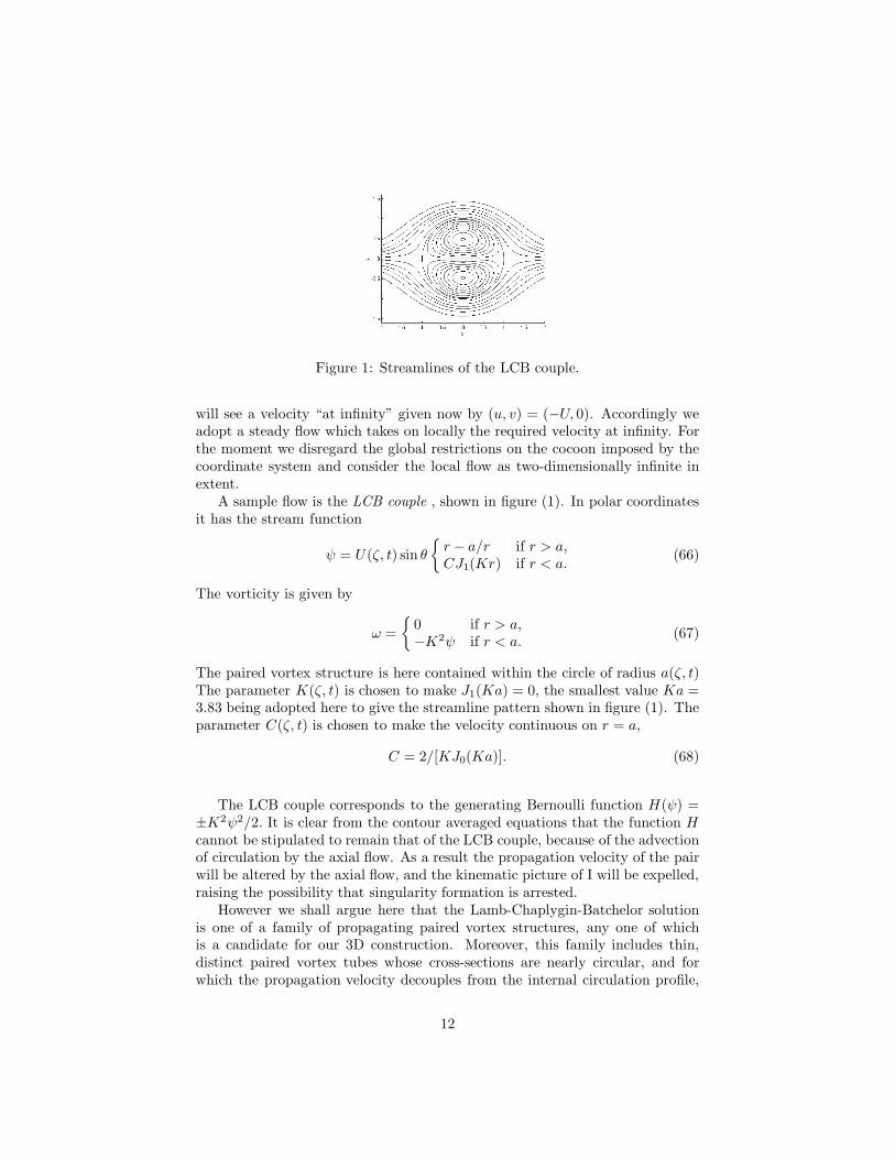
Figure 1: Streamlines of the LCB couple.

will see a velocity “at infinity” given now by (u, v) = (−U, 0). Accordingly weadopt a steady flow which takes on locally the required velocity at infinity. Forthe moment we disregard the global restrictions on the cocoon imposed by thecoordinate system and consider the local flow as two-dimensionally infinite inextent.

A sample flow is the LCB couple , shown in figure (1). In polar coordinatesit has the stream function

ψ = U(ζ, t) sin θ

{

r − a/r if r > a,CJ1(Kr) if r < a.

(66)

The vorticity is given by

ω =

{

0 if r > a,−K2ψ if r < a.

(67)

The paired vortex structure is here contained within the circle of radius a(ζ, t)The parameter K(ζ, t) is chosen to make J1(Ka) = 0, the smallest value Ka =3.83 being adopted here to give the streamline pattern shown in figure (1). Theparameter C(ζ, t) is chosen to make the velocity continuous on r = a,

C = 2/[KJ0(Ka)]. (68)

The LCB couple corresponds to the generating Bernoulli function H(ψ) =±K2ψ2/2. It is clear from the contour averaged equations that the function Hcannot be stipulated to remain that of the LCB couple, because of the advectionof circulation by the axial flow. As a result the propagation velocity of the pairwill be altered by the axial flow, and the kinematic picture of I will be expelled,raising the possibility that singularity formation is arrested.

However we shall argue here that the Lamb-Chaplygin-Batchelor solutionis one of a family of propagating paired vortex structures, any one of whichis a candidate for our 3D construction. Moreover, this family includes thin,distinct paired vortex tubes whose cross-sections are nearly circular, and forwhich the propagation velocity decouples from the internal circulation profile,

12

Figure 2: Streamlines of the paired vortex structure described by (136) and(137), 2πUL = Γ, R = .2L. The vortices are shaded.

approximately. In this limit the vorticity is confined to symmetrically placedcores of order R say, placed a distance L apart. If this separation o scalespersists, the pair propagates essentially as paired line vortices. In a framestationary with the advancing pair, one sees a region of fluid which is carriedwith the pair and where the flow is irrotational, see figure 2. The structureof the cores can be studied analytically for small ε = R/L, and we show inappendix B that through order ε3 the boundary of the a vortex core relativetwo its center is given by

r/L = ε+ ε3 cos 2θ. (69)

Within the core we have to this approximation

ψ = − Γ

2π

[ J0(kr)

kRJ1(kR)+ ε2

J2(kr)

J2(kR)cos 2θ

]

, (70)

where kR = 2.4048... is the first zero of J0. The velocity of the pair is thengiven by

U = − Γ

2πL. (71)

We now propose to treat each then vortex as circular, in which case thesymmetrized model acquires a new symmetry and becomes solvable in classicalterms.

3 Development of the s- independent singularity

in a symmetrized model

We consider a paired vortex structure modeled in each section by two circularvortex patches of radius R0(ζ, τ), see figure (2). We look for a fixed point ofthe system, i.e. we assume no dependence upon the local time s. In the upperdisc, we have the following problem. Let re = τγR,w = τ−γW, reve = Γ, ue =−reUtU−1 + τγ−1U . We also now take L = λτγ . Then we have

γW + (1 + γ)σWσ − (1 + γ)σgσg−1RWR

13

+g−2WWσ + UWR + g−2Pσ + 2(γ + (1 + γ)σgσg−1)W = 0, (72)

(1 + γ)σΓσ − (1 + γ)σgσg−1RΓR + g−2WΓσ + UΓR = 0, (73)

PR = Γ2/R3, (74)

g−2Wσ + R−1(RU)R = 0. (75)

We require that, on R = R0(σ), we have

Γ(R0, σ) = 2πλg(σ). (76)

The issue is, does a solution to this problem exist? We need to solve forW,Γ, P,U as functions of σ, R, for which we have four equations, then solve forR0(σ) to satisfy the last condition.

4 A one-dimensional model of the thin vortex

One-dimensional models of thin vortices with axial flow have proven extremelyuseful for analyzing vortex dynamics, see e.g. [Moore & Saffman (1972)]. Wetherefore turn now to such a model in the context of paired vortices. In thethin-tube limit, the vortices may be treated separately as filaments carryingconstant circulation. The variation of cross-sectional area with axial flow hasbeen discussed in a one-dimensional setting by [Lundgren & Ashurst (1989)],and our model will be closely related to theirs, but with emphasis now on theterms due to the motion and metric of the coordinate system.

The one-dimensional model of the symmetrized vortex with circular stream-lines involves an axial flow w(ζ, t0), a cross-sectional area a(ζ, t0), and a “pres-sure force” f(ζ, t0). (We adopt these symbols locally for this model only). Wehave the equations

a(wt0 +wwζ) + fζ − 2Uκwa = 0, at0 + (wa)ζ − Uκa = 0. (77)

The “2” appearing in the first equation, in place of the “1” in (63) comes fromthe way the continuity equation is used in the derivation. The pressure forceincrement df is an average of all pressure forces on a small piece of the tube.Within the tube, the pressure satisfies

∂p

∂r= v2

θ/r. (78)

If one integrates this over the cross section, using the leading term of (70), thenet force on the section has the form Γ2 times a function of kR, that is to saytimes a constant. That this is generally true follows from a simple dimensionalargument. As the tubes stretch, the pressure distribution is determined solelyby the local core area A and the total circulation Γ of the section. Dimensionallythe, p = Γ2A−1 times a function of ξ/

√

(A), η′√A. Integrating of the core gives

a multiple of Γ2.

14

Thus there is know contribution from internal pressure forces on the ends ofthe piece of tube to the force increment df . As was noted by [Lundgren & Ashurst (1989)],the only contribution to df comes from the pressure force on the side wall of hepiece of tube. Integrating (78) from R to ∞ we obtain

df = − Γ2

8π2R2da = −Γ2

8πd lna. (79)

Thus the axial momentum equation is

wt0 +wwζ +Γ2

8π(1/a)ζ − 2Uκw = 0. (80)

We now pass to the similarity form of our singular flow, assuming no vari-ation of the variables with s. We then have, if a = v−1, and we set v =τ−2γV (τ, σ), w = τ−γW (τ, σ),

(2γV + µσVσ)g2 +WVσ − VWσ − 2(γg2 + µσggσ)V = 0, (81)

(γW + µσWσ)g2 +WWσ +Γ2

8πVσ + 4(γg2 + µσggσ)W = 0. (82)

4.1 Analysis of the model

We first recall the asymptotics of g as established in I. 2 For large σ,

g ∼ [√

2µσ]−γ

1+γ − γ

2µ[√

2µσ]−( 2+γ

1+γ) + . . . . (83)

For small σ,g ∼ 1 − γ(1 + γ)σ2 + . . . . (84)

Since the tube must have area at σ = 0 we may assume limσ→0 V = V0 > 0.The, from (81), assuming V,W are analytic in σ at σ = 0, and that V has onlyeven powers of σ in its power series, we see that

V0Wσ ∼ 4γ(1 + γ)(1 + 2γ)σ2V0, (85)

so that , since necessarily W (0) = 0,

W ∼ 4γ(1 + γ)(1 + 2γ)σ3/3, σ→ 0. (86)

It is interesting that this flux is positive, away from the developing singularity,indicating that the squeezing down by stretching is beating the effect of pressureforces near σ = 0.

It now follows from (86), (82), and the expansion of g that

Γ2

8πVσ ∼ −(8γ + 3)(4γ)(1 + γ)(1 + 2γ)σ3. (87)

2The case we treat here for the function g is β = 2,A = 1, µ = 1 + γ. To restore the A

in what follows one need only replace σ by Aσ. This step will be needed to maintain correctdimensionality.

15

Thus

V ∼ V0 −8π

Γ2(8γ + 3)γ(1 + γ)(1 + 2γ)σ4 , (88)

so that tube area is increasing as σ increases from 0.Turning now to the behavior for large σ, in order that the asymptotic form of

the vorticity becomes independent of time we need W ∼ c1g, V ∼ c2g2, σ → ∞

at least in leading order, g ∼ O(σ−γ

1+γ ). Let us say that a term has falloff k ifit is proportional to σ−k to leading order. Then the terms WVσ −VWσ in (81),taken together, has falloff 4γ+1

γ+1 , while the last term in (81) has falloff 4γ+2γ+1 .

Thus the latter term is asymptotically negligible. Therefore (2γV + µσVσ)g2

must have falloff 4γ+1γ+1 , implying that

V ∼ c1σ−( 2γ

γ+1) + c2σ

−( 2γ+1

γ+1) + . . . . (89)

Similarly the Vσ term in (82) has falloff 3γ+1γ+1 , and the last term of (82) has

falloff 2, and this is greater than 3γ+1γ+1 since γ < 1. Thus the latter term is

negligible. Suppose now that the first term of (82) is also negligible. Then wewould have

1

2W 2 +

Γ2

8πV ∼ 0, σ → ∞. (90)

This is impossible since area cannot be negative. Thus the falloff of Vσ mustequal the falloff of the first term of (82). This requires

W ∼ d1σ−( γ

γ+1) + d2σ

−1 + . . . . (91)

Note that in each case the following term is smaller by the factor σ−1

γ+1 .Then (82) yields

(1 + γ)1

1+γ

γ21+2γ

1+γ

d2 + d21/2 +

Γ2

8πc1 ∼ 0, (92)

implying d2 < 0.

4.2 Numerical solution

The one-dimensional numerical problem which must be solved to insure theexistence of the needed fixed point of the generalized system will now be sum-marized. The system is most conveniently solved using g in place of σ as theindependent variable. Also Γ2/8π may be removed by V → 8πV/Γ2, equivalentto setting Γ =

√8π leaving Vg=1 as the only parameter. The the equations are

then

dV

dg= (W + µσg2)FV/D+GVW/D,

dW

dg= −FV/D+ (W + µσg2)GW/D,

(93)

16

Figure 3: The solutions of (93), (98) for various V0, γ = .6.

where

σ(g) =1√2µg−µ/γ

√

1 − g2/γ , (94)

F = 2µσg, G = −5γg2/g′ + 4µσg, (95)

g′(g) =−2γµσg3

1 + 2σ2µ2g2, (96)

D = (W + µσg2)2 + V. (97)

The boundary conditions are

V (0) = W (0) = 0, V (1) = V0 > 0,W (1) = 0. (98)

The necessary integral curves are easily found numerically by shooting fromg = 1 and are shown in figure 3. Note that the axial flow is always non-negative,never toward the singularity. This, and the smoothness of the integral curves,insures the validity of the one-dimensional model and is strongly suggestive ofa well behaved fixed point for the generalized system in the thin tube limit.

4.3 The outer potential flow

The total flow fieldin the vicinity of the vortex pair includes the component ofue given by −U−1Utre, which must be matched with an extgernaal potentialflow. The potential of the outer flow, denoted by φout, can be derived as follows.

17

In the matching region the votices a locally thin ζ, re may be replace by z, r,the local cylindrical coordinates. The we require

dφout/dr ∼ − rτ

(γ + µσgσ/g), r → 0. (99)

We may represent φout as the Laplace integral

φout =

∫

∞

0

e−kzF (k)J0(kr)dk. (100)

The matching requires

∫ ∞

0

e−kζk2F (k)dk =1

τ(γ + µσgσ/g). (101)

Thus

k2F (k) =1

2πiτ

∫

B

ekζ(γ + µσgσ/g)dζ, (102)

where B denotes the Bromwich path in the complex ζ plane. This can be written

k2F (k) =1

2πiτ

∫

B

ekζ[ γG2/γ

1 + γ − γG2/γ

]

dζ, (103)

where G(ζ) satisfies

ζ =τ1−γ

√2µ

[

G1−1/γ√

1 −G2/γ − 2

∫ G

1

u−1/γ√

1 − u2/γdu]

. (104)

Two points should be noted about this outer flow: (1) We have taken theζ-axis to be a straight line. This is valid in an intermediate region distant fromthe center vortex, i.e.

√

ξ2 + η2 � τγ but at a distance small compared toκ−1 ∼ τ1−γ . To study the irrotational outer flow at distances O(κ−1) from thecenter vortex we must take into account the curvature of the center vortex. (2)The pressure contributed by the outer potential vortex , at the vortex cores, isnegligible compared to that already considered in our one-dimensional modelof the cores. This pressure force, coming from an integral over the externalvortex velocity involving the integrand v2

θ/r, was of order τ−2γ By contrast theradial velocity component is O(τγ−1) when r ∼ τγ , contributing only orderτ2γ−1 to the pressure. Similarly the ζ component of velocity in the outer flowis O(τ3γ−2) when r ∼ τγ , and this is again o(τ−γ) when 1/2 < γ < 1. Finallythe time derivative of the potential, a final contributor to the pressure at thecore vortices, is of our τ2γ−2 when r ∼ τγ , again being o(τ−2γ).

4.4 Construction of the singularity

We have carried out here an analysis of the asymptotics of the singular flow, andhave made use of a one-dimensional model of the vortex cores. Although not arigorous proof of blow-up, we find no inconsistencies in the present construction,

18

which would rule out the existence of a singular flow in three dimensions. Onthe other hand we have not explicitly dealt with the finiteness of the dynamicalcocoon, which was needed only to prevent a singularity in the coordinate systemfrom entering the computational domain. To achieve full consistency we can,for example, impose an artifical stress-free cylindrical boundary, centered at thecenter vortex and of radius 1

2κ−1. Boundary conditions at this outer bound-

ary are then those of a rigid stress-free boundary. Imposing those conditionswould affect our flow by asymptotically negligible amounts as τ → ∞ in theneighborhood of the dynamic cocoon at distances small compared to κ−1. Thesingularity is thus asymptotically exact even with a proper outer boundary. Onecan imagine a procedure of approximation of the exact initial condition for theblow-up, as follows. With the cocoon imposed let the flow proceed as far intothe singularity as desired. Then remove the cocoon boundary, add a smoothextension of the outer flow to fill all space, and use this as an initial conditionfor a reverse flow. That is, reverse all velocities and run forwards in time forthe same elapsed time as in the approach to the singularity. In this way a se-quence of approximate initial conditions uk(T ) are obtained, representing as kincreases a closer and closer approach to blow-up. Because of the asymptoticconsistency of the construction, we conjecture that this sequence will convergeto a flow which is an example of an initial condition filling 3D space havingbounded, continuous vorticity, producing blow-up in finite time.

A final bit of surgery is needed to eliminate infinite energy in the initialcondition. Note that since only finite stretching is involved in the blow-up, onecan say that only a finite amount of kinetic energy is associated with the fluidparticipating in the blow-up. At this point, however, we note that a suitablevalue of γ, namely γ = (1 +

√19)/9 = .5954..., may be picked so that three

copies of the singularity may be arranged so that the center vortices will matchwith the sides of an equilateral triangle. Then in the neighborhood of eachvertex we have a copy of the self-similar singular flow, and finite total energy ofthe system of three participating singular regions.

5 Discussion

5.1 General remarks

The thrust of the present paper amounts to the proposition that the presentconstruction yields an acceptable example of Euler blow-up in three dimensions.It is acceptable in the sense that only a finite amount of vortex stretchingoccurs during the blow-up. Other analytical approaches suffer from the factthat infinite kinetic energy occurs in the flow comprising the set of singular

points. Such infinite-energy solutions tell us nothing about the behavior ofEuler flows of finite kinetic energy in a bounded domain.

The present part represents the second step toward verification of our propo-sition. It falls short of a complete verification, even in the weak sense of formaltheoretical fluid dynamics, in that we have utilized a one-dimensional model

19

of tube dynamics when in fact the problem is two-dimensional. However therobustness of 1-D theory for slender vortex tubes of near circular cross sectionmakes for a stronger case than might be otherwise accepted. There is no indica-tion that the 2D analysis would go much further that verifying the correctnessof the one-dimensional approximation.

We have also used the asymptotic form of the thin-tube LCB solution ratherthan an exact form. The issue of existence of a full family of LCB-like Eulerflows, and the size of this family, is an interesting question in itself, which toour knowledge has not been answered.

5.2 Stability of the singular flow

We do not consider here in any detail the important question of the stabilityof the proposed singular flow. Like most Euler flows, it is likely to be un-stable. If this were indeed the case, then these singularities are in principleunobservable even in a perfect fluid, a point that renders computational ap-proaches of doubtful use. Three-dimensional instability of paired vortices hasbeen observed experimentally by [Leweke & Williamson (1998)]. The modes ofinstability they find appear to have their origin in the three-dimensional el-liptic instability of 2D vortex cores, see [Pierrehumbert (1986), Bayly (1986)],which makes the instability sensitive to stretching of the votices. Instability inthe zeroth-order solution here means that the growth is on a time scale t∗(τ )such that dt∗/dτ = τ−2γ, the poser being that needed to make τ derivatives inthe momentum equation of the same order as the advective acceleration. Thust∗(τ ) = τ1−2γ. Thus, since γ > 1/2, t∗ → ∞ as τ → 0. Thus the instabilityhas “infinite time” to grow, with complete disruption of the singularity the in-evitable result. This underscores the importance of looking for the “fixed pointsolution”, by which we mean a steady zeroth-order Euler flow together withindependence of the dynamic variables on the logarithmic time scale s.

Associated with the question of instability is the issue of the “density” ofinitial conditions producing blow-up in some function space of allowable initialconditions. On interesting prospect is that both issues may involve the down-stream ×-type neutral (stagnation) point of the paired vortex flow. The outerstreamline boundaries of the closed region are stable manifolds of this neuralpoint. Any perturbation of the manifolds preserving the volume of the closedregion leads to mixing of fluid interior and exterior to these manifolds. Eventu-ally these disruptions would extract vorticity from the cores and break up thepair, see figure 4. The perturbations of the manifold would be introduced byperturbations of the vortical cores, see figure 4. Note that this is a purely 2Dinstability of the zeroth-order flow, and is insensitive to stretching.

The “neutral-point instability” just described would explain the difficulty inidentifying a blow-up initial condition , as follows. Let us introduce a measureon the set of initial condition defined by the boundaries of the vortical cores.The singular conditions, i.e. the “fixed point” contours will lie between to circlescentered at the vortex center. Any other simple closed contour around the innerboundary of this annulus constitutes a possible initial condition when extended

20

Figure 4: A possible instability of the zeroth-order solution. Only the uppervortex is shown.

in our construction along the center vortex. Now there will generally be a setof fixed point contours, parametrized by the area enclosed. But for each sucharea, these is at the very minimum a one (real) parameter family of contours,given say by taking the maximum excursion radially from the correspondingfixed point contour. A measure on all contours will therefore leave the fixed-point contours as measure zero. Thus the contours leading to blow-up in ourconstruction constitute a set of measure zero in the space of feasible contours.

5.3 The impossibility of the singularity in viscous flows

The important question of singularities of solutions of the Navier-Stokes equa-tions leads, in the present construction, to a negative result. The question isintriguing nonetheless, because the viscous term ν∇2u, which is dominated hereby ν(uξξ + uηη), has the same order as the acceleration in our zeroth-order so-lution. However this 2D Navier-Stokes equation can have no steady solution infinite space. Thus there would have to be evolution on the time scale t∗ justintroduced. The ultimate exponential decay occuring in the Stokes limit thentranslates to super-exponential decay in τ , overwhelming the algebraic growthassociated with the singularity of vorticity.

This conclusion could not be drawn if γ were to equal 1/2, but in that casethe Euler singularity cannot occur at least according to the present construc-tion. Nevertheless we suggest that viscous flows with structure approachingthat of the present Euler flows with γ = 1/2 would be able to amplify vorticitysignificantly, before saturating and decaying.

5.4 Comparison of this work with the construction of Sig-

gia and Pumir

In [Pumir & Siggia (1990)] a theory of singularity formation based upon self-stretching of paired vortices is developed. The pioneering construction proposedby Pumir and Siggia is similar in many respects to the present one. Howeverthere are important differences. In the first place, their proposal corresponds toour case γ = 1/2. It is for that reason that both Navier-Stokes and Euler flows

21

are considered in [Pumir & Siggia (1990)]. According to [Chae (2006)] this is anexample of self-similarity, where in fact an Euler singularity cannot exist. Theproblem one encounters when γ = 1/2, as indeed [Pumir & Siggia (1990)] knew,is that one could not guarantee the integrity of the vortex cores at the singularitytime. For example, paired vortices with radius of curvature κ are drawn toone another in the direction of the binormals with a velocity proportional toκ ln(κ/a) where a is a core radius of the vortex. In the present constructionthis velocity is O(τγ−1) and is negligible compared to the O(τ−γ) velocity ofthe vortex itself, but in [Pumir & Siggia (1990)] these velocities are comparable,with the possibility of core deformation as the vortices collide.

The main motivation of the present work is the kinematic singularity pre-sented in I, and Pumir and Siggia seem to have not been aware of that solutionof the equations of a line moving by the normal. However they do undertakelocal analysis of the collapse to the singularity using line vortices, and arrive at asimilar conclusion of formation of a point singularity with finite total stretching.

The research reported in this paper was supported by the National ScienceFoundation under KDI grant DMS-0507615 at New York University.

A Contour averaging

The function A(ψ, ζ, t) is the area enclosed by a contour have streamfunctionvalue ψ(ξ, η, ζ, t) at a fixed section ζ = constant of the dynamic cocoon. Usingthe contour average (35), we first establish the following properties:

〈1〉 = Aψ, 〈ψζ〉 = −Aζ , 〈ψt〉 = −At. (105)

The first expression follows from

δA = Aψδψ =

∮

δnds = δψ

∮

δn

δψds = δψ

∮

q−10 ds = δψ〈1〉. (106)

The second (and third) of (105) follow from differentiation of ψ for fixed ψ ands:

∂ψ

∂ζ

∣

∣

∣

ψ,s= 0 =

∂ψ

∂ζ

∣

∣

∣

n,s+ ψn

∂n

∂ζ

∣

∣

∣

ψ,s. (107)

Taking the contour average then gives

0 = 〈ψζ〉 +

∮

nζds = 〈ψζ〉 + +Aζ , (108)

establishing the result. Also we see that

〈ψξ〉 = 〈ψη〉 = 0. (109)

Indeed,∮

(u0, v0)/q0ds =

∮

(dx, dy) = (0, 0). (110)

22

We also observe the following useful identity:

∫ ∫

(·)dA =

∫

〈·〉dψ. (111)

This follows from dA = dsdn = dsdψ/q0.The differential operator D ≡ ∂t+w∂z+q1 ·∇ occurs in the right-hand side

of (32) and we need to compute the contour average of its action on ψ. (Hereand elsewhere we have written ∂t for ∂t0.) We have, using (105)

〈Dψ〉 = 〈ψt〉 +w〈ψζ〉 + 〈q1 · ∇ψ〉,

= −At −wAζ +

∮

q1 · nds,

−At −wAζ −∫ ∫

[wζ∣

∣

ξ,η− Uκ]dA. (112)

Using the chain rule and (105) we obtain

∫ ∫

wζ∣

∣

ξ,ηdA =

∫

〈wζ∣

∣

ψ+ ψζ

∣

∣

ξ,ηwψ

∣

∣

ζ〉dψ,

=

∫

(wζAψ −Aζwψ)dψ =

∫

∂(w,A)

∂(ζ, ψ)dψ. (113)

Combining these,

−〈Dψ〉 =

∫

0

[Aψt +wAψζ + Aψwζ − UκAψ]dψ = AψV. (114)

We now indicate the derivation of (37) from the contour average of the w-part of (32). (The derivation of (36) is similar.) Now the terms of F 1

w involvingu′ vanish by (109). The differentiation of w divides by the chain rule intodifferentiations at fixed ψ and wψ times differentiations of ψ. The latter areevaluated in terms of 〈Dψ〉. The only term needing discussion is 〈pζ〉. We writep = H − 1

2q20. Then, as in

∫ ∫

Hζ

∣

∣

ξ,ηdA =

∫

∂(H,A)

∂(ζ, ψ)dψ. (115)

To evaluate 〈q0 · q0

∣

∣

ξ,η〉 we observe

∫ ∫

∇2ψdA =

∫ ∫

HψdA =

∮

∇ψ · nds. (116)

Thus∫ ∫

∂Hψ

∂ζ

∣

∣

∣

ξ,ηdA = 〈q0 · q0

∣

∣

ξ,η〉 =

∫

∂(Hψ, A)

∂(ζ, ψ)dψ. (117)

These results combine to yield (37).

23

B Derivation of the first few terms of the thin-

tube solution

We locate the tube centers at z = ±iL/2 in a frame in which they are atrest. The velocity at infinity is (U, 0), U < 0, and the upper vortex has positivecirculation, see figure 6. With our definition of ψ the complex potential valid inthe irrotational region is

w(z) = φ(x, y) − iψ(x, y) = Uz − iΓ

2πlog(z − iL/2) +

iΓ

2πlog(z + iL/2)

+A+ iB

z − iL/2+

A − iB

z + iL/2+O(z−2). (118)

Within the upper vortex we take

ψin = CJ0(kr) + (D cos θ+ E sin θ)J1(kr) + F + . . . . (119)

Here k, A, B, ..., F are real constants. We assume the boundary of the uppervortex is given by |z − iL/2| = R + α cos θ + β sin θ + . . .. Here θ is the polarangle with respect to the center of the upper vortex.

Now from (118) we have, near the upper vortex,

ψout = −U(y−L/2)−UL/2+Γ

2πln(|z−iL/2|/L)−Γ(y − L/2)

2πL−= A + iB

z − iL/2+. . . .

(120)To make ψin = constant on |z − iL/2| = R + α cos θ + β sin θ we see thatnecessarily J0(kR) = 0, and take kR as the first zero of this Bessel function. Itthen follows that, to lowest order,

Γ = −2πkRCJ1(kR). (121)

Thus, again to lowest order

F =Γ

2πln(R/L) − UL/2. (122)

The second-order calculations involve cos θ, sin θ. To make ψin constant onthe vortex boundary we must have

−CJ1(kR)(α cos θ + β sin θ) + (D cos θ + E sin θ)J1(kR) = 0. (123)

ThusD = Cα,E = Cβ. (124)

To make ψin = ψout on the vortex boundary to second order, we must have

−UR sin θ +Γ

2πR(α cos θ + β sin θ) − ΓR sin θ

2πL− B cos θ −A sin θ

R= 0. (125)

24

To make ψr continuous on the boundary we must have

−UR sin θ − Γ

2πR(α cos θ + β sin θ) − ΓR sin θ

2πL+B cos θ −A sin θ

R= 0. (126)

It follows that

U =−Γ

2πL,A = −Γβ, B = αΓ, (127)

We see that α, β remain arbitrary, but these are perturbations association withsmall shifts of the center position of the vortex. We may therefore set A = B =D = E = α = β = 0, and take |z − iL/2| = R+ α2 cos 2θ+ β2 sin 2θ+ . . ., with

ψin = CJ0(kr) + (D2 cos 2θ + E2 sin 2θ)J2(kr) + F + . . . , (128)

w(z) = Uz − iΓ

2πlog(z − iL/2) +

iΓ

2πlog(z + iL/2)

+A2 + iB2

(z − iL/2)2+

A2 − iB2

(z + iL/2)2+ O(z−3). (129)

Now we have the condition analogous to (123):

−CkJ1(kR)(α2 cos 2θ + β2 sin 2θ) + (D2 cos 2θ+ E2 sin 2θ)J2(kR). (130)

ThusD2 = CkJ1(kR)α2/J2(kr), E2 = CkJ1(kR)β2/J2(kr). (131)

Also the streamfunction near the upper vortex is now

ψout = −U(y − L/2) − UL/2 +Γ

2πln(|z − iL/2|/L) − Γ(y − L/2)

2πL

− Γ

8πL2[x2 − (y − L/2)2] − B2 cos 2θ −A2 sin 2θ

|z − iL/2|2 + . . . . (132)

From the jump conditions at the vortex boundary we obtain the following con-ditions on the terms in cos 2θ, sin 2θ:

ΓR

2π(α2 cos 2θ+ β2 sin 2θ) − (B2 cos 2θ− A2 sin 2θ) =

R4

8πL2cos 2θ, (133)

ΓR

2π(α2 cos 2θ + β2 sin 2θ) − 2(B2 cos 2θ− A2 sin 2θ) = − R4

4πL2cos 2θ. (134)

Thus

α2 = R3/L2, B2 =3ΓR4

8πL2, A2 = β2 = 0. (135)

The second-order complex potential is therfore

w(z) = Uz − iΓ

2πlog(z − iL/2) +

iΓ

2πlog(z + iL/2)

+i3ΓR4

8πL2(z − iL/2)2− i

3ΓR4

8πL2(z + iL/2)2+O(z−3), (136)

and the boundary of the upper vortex is given by

r = R+R3

L2cos 2θ. (137)

25

References

[Majda & Bertozzi (2002)] Majda, Andrew J. & Bertozzi, Andrea L.

(2002) Vorticity and Incompressible Flow, Cambridge University Press.

[Childress (1985)] Childress, Stephen (1987) Nearly Two-dimensional solu-tions of Euler’s equations. Phys. Fluids, 30, 944–953.

[Pelz (2001)] Pelz, Richard B. (2001) Symmetry and the hydrodynamicblow-up problem. J. Fluid Mech. 444, 299–320.

[Kerr (2005)] Kerr, Robert M. (2005) Velocity and scaling of collapsing Eulervortices. Phys. Fluids 17 , 075103.

[Siggia (1985)] Siggia, Eric D. (1985) Collapse and amplification of a vortexfilament. Phys. Fluids 28, 794–805.

[Childress (2006)] Childress, Stephen (2006) On vortex stretching and theglobal regularity of Euler flows I. Axisymmetric flow without swirl, preprint.

[Batchelor (1967)] Batchelor, G.K. (1967) An introduction to Fluid Dynam-

ics, Cambridge.

[Milne-Thomson (1955)] Milne-Thomson, L.M. (1955) Theoretical Hydrody-

namics, McMillan.

[Pumir & Siggia (1990)] Pumir, Alain & Siggia, Eric (1990) Phys. Fluids

A2, 220–241.

[Constantin et al. (1996)] Constantin, Peter, Fefferman, Charles, &

Majda, Andrew J. (1996) Geometric constraints on potentially singularsolutions for the 3-D Euler equations. Commun. in Part. Diff. Eqns. 21 , 559– 571 .

[Deng et al.(2004)] Deng, Jian, Hou, Thomas Y., & Yu, Xinwei (2004)Geometric conditions on vorticity and blow-up of solutions of the 3D Eulerequations. Preprint

[Chae (2006)] Chae, Dongho (2006) Nonexistence of self-similar singularitiesfor the 3D incompressible Euler equations. Preprint.

[Frisch et al. (2003)] Frisch, U., Matsumoto, T.,& Bec, J. (2003) Singu-larities of Euler flow? Not out of the blue! J. Stat. Phys. 113, 761–781.

[Constantin (2004)] Constantin, Peter (2004) Some open problems and re-search directions in the mathematical study of fluid dynamics. Essay, availableonline.

[Beale, Kato & Majda (1984)] Beale, J.T., Kato, T., & Majda, A. (1984)Remarks on the breakdown of smooth solutions of the 3-D Euler equations.Commun. Math, Phys. 94, 61–66.

26

[Grad et al (1975)] Grad, H.,, Hu, P.H., and Stevens, D. (1975) Evolutionof plasma equilibrium. Proc. Nat. Acad. Sci. USA12, 3789-3793.

[Lamb (1906)] Lamb, H. (1955) Hydrodynamics (3rd edn.), Cambridge Univer-sity Press.

[Meleshko & van Heijst (1994)] Meleshko, V.V. & Heijst, G.J.F. (1994)On Chaplygin’s investigations of two-dimensional vortex structures in an in-viscid fluid. J. Fluid Mech. 272, 157–182.

[Chaplygin (1903)] Chaplygin, S.A. (1903) On case of vortex motion in fluid.Trans. Sect. Imperial Moscow Soc. Friends of natural Sciences 11, N 2, 11–14.See also Collected Works (1948), vol. 2, 155–165 (in Russian).

[Moore & Saffman (1972)] Moore, D.W. & Saffman, P.G. (1972) The mo-tion of a vortex filament with axial flow. Proc. R. Soc. London A 272, 407–429.

[Lundgren & Ashurst (1989)] Lundgren, T.S. & Ashurst, W.T. (1989)Area-varying waves on curved vortex tubes with application to vortex break-down. J. Fluid Mech. 200, 283–307.

[Leweke & Williamson (1998)] Leweke, T & Williamson. C.H.K. (1998)Cooperative elliptic instability of a vortex pair. J. Fluid Mech. 360, 85–119.

[Bayly (1986)] Bayly, B.J. (1986) Three-dimensional instability of ellipticalflow. Phys. Rev. Lett. 57, 2160.

[Pierrehumbert (1986)] Pierrehumbert, R.T. (1986) Universal short-waveinstability of two-dimensional eddies in an inviscid fluid. Phys. Rev. Lett.

57, 2157.

27