1

Constrained Gaussian Mixture Model Frameworkfor Automatic Segmentation of MR Brain Images

Hayit Greenspan Amit Ruf and Jacob Goldberger

Abstract— An automated algorithm for tissue segmentationof noisy, low contrast magnetic resonance (MR) images of thebrain is presented. A mixture model composed of a large numberof Gaussians is used to represent the brain image. Each tissueis represented by a large number of Gaussian components tocapture the complex tissue spatial layout. The intensity ofatissue is considered a global feature and is incorporated into themodel through tying of all the related Gaussian parameters.TheExpectation-Maximization (EM) algorithm is utilized to le arnthe parameter-tied, constrained Gaussian mixture model. Anelaborate initialization scheme is suggested to link the set ofGaussians per tissue type, such that each Gaussian in the sethas similar intensity characteristics with minimal overlappingspatial supports. Segmentation of the brain image is achieved bythe affiliation of each voxel to the component of the model thatmaximized the a-posteriori probability. The presented algorithmis used to segment 3D, T1-weighted, simulated and real MRimages of the brain into three different tissues, under varyingnoise conditions. Results are compared with state-of-the-artalgorithms in the literature. The algorithm does not use an atlasfor initialization or parameter learning. Registration pr ocessesare therefore not required and the applicability of the frameworkcan be extended to diseased brains and neonatal brains.

Index Terms— Image segmentation, MRI brain segmentation,Mixture of Gaussians, GMM, EM, Constrained model

I. I NTRODUCTION

Automatic segmentation of brain MR images to the threemain tissue types: white matter (WM), gray matter (GM)and cerebro-spinal fluid (CSF), is a topic of great importanceand much research. It is known that volumetric analysis ofdifferent parts of the brain is useful in assessing the progressor remission of various diseases, such as Alzheimer’s disease,epilepsy, sclerosis and schizophrenia [21].

A variety of segmentation schemes exist in the literature.As it is very difficult to estimate automatic or semi-automaticsegmentation results against an in-vivo brain, manual segmen-tation by experts is still considered to be the “gold standard”or “ground truth” for any automated algorithm. However,manual partitioning of large amounts of low-contrast/low-SNR brain data is strenuous work and is prone to largeintra- and inter-observer variability. Fully automated intensity-based algorithms, on the other hand, exhibit high sensitivityto various noise artifacts, such as intra-tissue noise, inter-tissue intensity contrast reduction, partial-volume effects and

H. Greenspan is with the Tel-Aviv University, Tel Aviv 69978, Israel. E-mail: hayit@eng.tau.ac.il

A. Ruf is with the Tel-Aviv University, Tel Aviv 69978, Israel. E-mail:amitruf@gmail.com

J. Goldberger is with the Bar-Ilan University, Ramat-Gan 52900, Israel.E-mail: goldbej@eng.biu.ac.il

others [16]. Reviews on methods for brain image segmentation(e.g.,[21]) present the degradation in the quality of segmen-tation algorithms due to such noise, and recent publicationscan be found addressing various aspects of these concerns(e.g. partial-volume effect quantification [7]). Due to thearti-facts present, classical voxel-wise intensity-based classificationmethods, such as K-means modeling and Mixture of Gaussiansmodeling (e.g., [25],[11] ), may give unrealistic results,withtissue class regions appearing granular, fragmented, or violat-ing anatomical constraints.

Incorporating spatial information via a statistical atlaspro-vides a means for improving the segmentation results (e.g.[22], [13], [18]). The statistical atlas provides the priorprob-ability for each pixel to originate from a particular tissueclass. Algorithms that are based on the maximum-a-posteriori(MAP) criterion utilize the atlas information in the algorithmiterations to augment the information in the presence of noisydata. Co-registration of the input image and the atlas, acomputationally intensive procedure, is critical in this scenario[23]. It is important to note that the quality of the registrationresult is strongly dependent on the physiological variabilityof the may converge to an erroneous result in the case of adiseased or severely damaged brain. Moreover, the registrationprocess is applicable only to complete volumes. A single slicecannot be registered to the atlas, thus, cannot be segmentedusing these state-of-the-art algorithms.

An additional conventional method to improve segmentationsmoothness and immunity to noise is to model neighboringvoxels interactions using a Markov Random Field (MRF)statistical spatial model [13], [27], [9]. Smoother structuresare obtained in the presence of moderate noise as long asthe MRF parameters controlling the strength of the spatialinteractions are properly selected. Too high a setting can resultin an excessively smooth segmentation and a loss of importantstructural details [15]. In addition, MRF-based algorithmsare computationally intractable unless some approximation isused which still requires computationally intensive algorithms.Algorithms that use deformable models to incorporate tissueboundary information [19] imply inherent smoothness butrequire careful initialization and precisely calibrated model pa-rameters in order to provide consistent results in the presenceof a noisy environment. Several works can be found in theliterature, such as fuzzy connectedness segmentation methods,that attempt to provide an alternative to the MRF modeling(e.g. [20], [26]. In [26], as in many other works, there stillseems to be a need for a large number of parameters for thetask.

The objectives of the current work are threefold: 1) incorpo-

2

Preprocessing

Features

Extraction

(I,X,Y,Z)

Learning

The CGMM

parametersSegmentation

T1-weighted

Fig. 1. Schematic description of the CGMM segmentation framework

rate spatial information within a statistically-based model in asimple and intuitive way, for both localization and smoothing;2) achieve robust segmentation on real data along with strongresistance to noise, and 3) achieve accurate segmentation evenin cases in which an atlas is not available or appropriatefor the task. A robust, unsupervised, parametric method forsegmenting 3D (or 2D) MR brain images with a high degreeof noise and low contrast, is presented1. We refer to theproposed framework as theConstrained Gaussian MixtureModel (CGMM) framework. In this framework, each tissueis modeled with multiple four-dimensional Gaussians, whereeach Gaussian represents a localized region (3 spatial features)and the intensity characteristic per region (T1 intensity fea-ture). Incorporating the spatial information within the featurespace is novel, as is using a large number of Gaussians perbrain tissue to capture the complicated spatial layout of theindividual tissues. Note that models to-date utilize the intensityfeature only and use a single Gaussian per tissue type (e.g.[25], [18], [13]). The intensity of a tissue is considered a globalfeature and is incorporated into the model via parameter-tying:the intensity parameter of all the clusters that are relatedtothe same tissue, is essentially the same, and is considered asa single parameter that appears several times in the model.The Expectation-Maximization (EM) algorithm is utilized tolearn the parameter-tied, constrained Gaussian mixture model(GMM). An elaborate initialization scheme is suggested to linkthe set of Gaussians per tissue type, such that each Gaussianin the set has similar intensity characteristics with minimaloverlapping spatial supports. Two key features of the proposedframework are: 1) combining global intensity modeling withlocalized spatial modeling, as an alternative scheme to MRFmodeling, and 2) segmentation is entirely unsupervised; thuseliminating the need for atlas registration, or any intensitymodel standardization. The paper is organized as follows: adetailed description of the proposed framework is providedin Section II. Algorithm validation on both simulated andreal brain volumes is presented in Section III. Discussion andconclusions are presented in Section IV.

II. T HE CGMM SEGMENTATION FRAMEWORK

In this section a detailed description of the segmentationframework is presented. Figure 1 illustrates the four majorstages of the framework. In a preprocessing stage the brainregion is extracted and intensity inhomogeneities (bias) arecorrected (based on [13] as described in section III). In afeature-extraction stage a four-dimensional feature vector is

1Preliminary results of the study presented in this paper appeared in [24].

extracted for each voxelv. The main feature is the voxel in-tensity, denoted byvI . In order to include spatial information,the (X, Y, Z) position is appended to the feature vector. Weuse the notationvXY Z = (vX , vY , vZ) for the three spatialfeatures.

The set of feature vectors extracted per volume is denoted by{vt | t = 1, ..., T} whereT is the number of voxels. The set offeature-vectors is input to the learning stage of the framework,in which a variation on the GMM is utilized to representthe intensity and spatial characteristics of the input image.Details of the probabilistic model and its parameter learningvia the EM algorithm, are described in sections II-A and II-B.Segmentation of the brain image based on the learned modelis described in section II-C. A model initialization schemeisdescribed in section II-D.

A. The Probabilistic Model

The complex spatial layout of an MRI brain image providesa challenge for conventional GMM modeling schemes. Inorder to accommodate the spatial complexity, we model animage as a mixture ofmanyGaussians:

f(vt|Θ) =

n∑

i=1

αifi(vt|µi, Σi) (1)

such thatvt is the feature vector associated with thet-th voxel,n is the number of components in the mixture model,µi

andΣi are the mean and the covariance of thei-th Gaussiancomponentfi, and αi is the i-th mixture coefficient. Thespatial shape of the tissues is highly non-convex. However,since we use a mixture of many components, each Gaussiancomponent models a small local region. Hence, the implicitconvexity assumption induced by the Gaussian distributionisreasonable (and is empirically justified in the next section).

The high complexity of the spatial structure is an inherentpart of the brain image. The intra variability of the intensityfeature within a tissue (bias) is mainly due to artifacts of theMRI imaging process and once eliminated (via bias-correctionschemes) is significantly less than the inter-variability amongdifferent tissues. It is therefore sufficient to model the intensityvariability within a tissue by a single Gaussian (in the intensityfeature). To incorporate this insight into the model, we furtherassume that each Gaussian is linked to a single tissue andall the Gaussians related to the same tissue share the sameintensity parameters.

Technically, this linkage is defined via a grouping function.In addition to the GMM parameter setΘ, we define a groupingfunction π : {1, ..., n} → {1, ..., k} from the set of Gaussians

3

to the set of tissues. We assume that the number of tissues isknown and the grouping function is learned in the initializationstep. The intensity feature should be roughly uniform in thesupport region of each Gaussian component, thus, each Gaus-sian spatial and intensity features are assumed uncorrelated.The above assumptions impose the following structure on themean and variance of the Gaussian components:

µi =

µXY Zi

µIπ(i)

, Σi =

ΣXY Zi 0

0 ΣIπ(i)

(2)

whereπ(i) is the tissue linked to thei-th Gaussian componentand µI

j and ΣIj are the mean and variance parameters of all

the Gaussian components that are linked to thej-th tissue.The main advantage of the CGMM framework is the ability

to combine, in a tractable way, a local description of thespatial layout of a tissue with a global description of thetissue’s intensity. The multi-Gaussian spatial model makesour approach much more robust to noise than intensity-basedmethods. Note that no prior atlas information is used in themodeling process. Figure 2 illustrates the concept of com-bining local spatial modeling with global intensity modeling.A (2σ) spatial projection of the region-of-support for eachGaussian in the model is shown. Different shades of grayrepresent the three distinct tissues present.

Fig. 2. Modeling each of the three tissues with multiple Gaussians. Gaussianswith the same gray level share the same tissue label.

B. Learning the CGMM parameters

The EM algorithm [4] is utilized to learn the model pa-rameters. In the proposed framework, Gaussians with thesame tissue-label are constrained to have the same intensityparameters throughout. A modification of the standard EMalgorithm for learning GMM is required, as shown in thefollowing equations. The expectation step of the EM algorithm

for the CGMM model is (same as the unconstrained version):

wit = p(i|vt) =αifi(vt|µi, Σi)

∑n

l=1 αlfl(vt|µl, Σl)(3)

i = 1, ..., n t = 1, ..., T

We shall use the abbreviations:

ni =

T∑

t=1

wit i = 1, ..., n (4)

kj =∑

i∈π−1(j)

ni j = 1, ..., k

such thatni is the expected number of voxels that are relatedto the i-th Gaussian component,π−1(j) is the set of all theGaussian components related to thej-th tissue andkj is theexpected number of voxels in that tissue. The maximizationin the M-step is done given the constraint on the intensityparameters:

αi =ni

ni = 1, ..., n (5)

µXYZi =

1

ni

T∑

t=1

witvXYZt

ΣXYZi =

1

ni

T∑

t=1

wit

(

vXYZt − µXYZ

i

) (

vXYZt − µXYZ

i

)⊤

µIj =

1

kj

∑

i∈π−1(j)

T∑

t=1

witvIt j = 1, ..., k

ΣIj =

1

kj

∑

i∈π−1(j)

T∑

t=1

wit

(

vIt − µI

j

)2

The grouping functionπ that links between the Gaussiancomponents and the tissues is not altered by the EM iterations.Therefore, the affiliation of a Gaussian component to a tissueremains unchanged. However, since the learning is performedsimultaneously on all the tissues, voxels can move betweentissues during the iterations. Figure 3 shows the 2σ initialregion support (a) versus the final region support (b) of theGaussians, on the same synthetic image, after seven EMiterations.

(a) (b)

Fig. 3. Initial (a) and final (b) region support for all the Gaussians afterseven EM iterations. Different shades of gray present different tissue labels.

4

C. Image Segmentation

A direct transition is possible between the estimated imagerepresentation and probabilistic segmentation. If the represen-tation phase is a transition from voxels to clusters (Gaussians)in feature space, the segmentation process can be thought ofasforming a linkage back from the feature space to the raw inputdomain. Each voxel is linked to the most probable Gaussiancluster, i.e. to the component of the model that maximizes thea-posteriori probability. In GMM that are based on intensityonly and in which a single Gaussian models a particularclass, the selection of the Gaussian with the highest posteriorprobability for each voxel immediately produces the requiredsegmentation into one of the different tissues. The CGMMmodel uses multiple Gaussians for each tissue. Thus we needto sum over the posterior probabilities of all the identicaltissueGaussians to get the posterior probability of each voxel tooriginate from a specific tissue. Bayes rule implies that theposterior probability for a pixel to be linked to thej-th tissueis:

p(tissuej |vt) =

∑

i∈π−1(j) αifi(vt|µi, Σi)∑n

i=1 αifi(vt|µi, Σi)(6)

j = 1, ..., k , t = 1, ..., T

Hence the most likely tissue for thet-th voxel is:

tissue-labelt = argmaxj∈{1,...,k}

p(tissuej |vt) t = 1, ..., T (7)

such that tissue-labelt ∈ {1, ..., k} is one of the tissues. Thelinkage of each voxel to a tissue label provides the finalsegmentation map.

D. Model Initialization

The EM algorithm requires appropriate initialization, as itis notoriously known to get stuck on local maxima of thelikelihood function. In the multi-component CGMM modelthe problem is even more severe. A novel semi-supervisedtop-down initialization method is used in the current work,utilizing a-priori knowledge about the number of tissues ofinterest. The initialization is a dual step procedure, performedon a down-sampled version of the brain volume in order todecrease processing time. In the first step, intensity-basedK-means clustering extracts a rough segmentation into sixtissue classes: WM, GM, CSF, as well as three additionalclasses which take care of partial-volume effects as well asany other-than brain information that may be present in theimage (see also [14]). It is assumed that the CSF class isof lowest intensity. In most cases, the brain image is cleanedsufficiently in the pre-processing stage and the WM class is theclass with highest intensity. Cases exist in which fat residuesof bright values, remain in the image. For this reason, thebrightest class as well as its consecutive (less bright) classesare considered to belong to the WM category, until the numberof WM voxels, in all the selected classes, is larger than a userdefined threshold (MinWMfrac). All the voxels that were notlabelled as WM or CSF, are labelled as GM voxels. Thisrough but important initial clustering determines an initialgroup of voxels that belong to each tissue. An example for the

segmentation achieved on a 2D image is shown in Figure 4(a)where the two gray levels represent the two classes present.The segmentation is used as a masking procedure (Figure 4(b))that makes is possible to work on each tissue separately (regionof interest is indicated in white).

The next step is a top-down procedure which propagatesthe tissue class information into the spatial space. Regionsare split iteratively until convex regions are found that aresuitable for Gaussian modeling. Each iteration of the spatialregion splitting algorithm involves the following steps:

• A 3D connected-components (CC) algorithm is used todefine distinct regions which should be modeled by oneor more Gaussians. Figure 4(c) shows the CC regions inshades of gray.

• Each CC region is encircled with the smallest ellipsoidpossible2. If the volume inside the ellipsoid, that isnotpart of the region, is higher than a user defined threshold(“OutliersThresh”) and the ellipsoid volume sup-ports more voxels than the defined threshold value ofminimum voxels per region (“MinPixThresh”), theregion is marked for further splitting. This process isillustrated in Figure 4(d), where the largest CC regionis encircled with a 2D ellipsoid.

• A marked region is further split using K-means on thespatial featuresonly, into 2-10 distinct (not necessarilyconnected) subregions, depending on the size of theellipsoid and the user defined threshold for the minimumsize of ellipsoid. Figure 4(f) illustrates splitting of twodistinct regions.

The splitting algorithm iteratively proceeds as long as at leastone region is marked for partitioning. Once the regions aredetermined, each region is modeled with a single Gaussian.The Gaussian’s spatial parameters (mean & variance) are esti-mated using the spatial features of the voxels supported by theregion inscribed in the ellipsoid, while the intensity parameteris estimated using all the voxels supported by all the regions ofthe same tissue. Thus, Gaussians of the same tissue receive thesame initial intensity parameter. Furthermore, each Gaussian istagged with a label that indicates its tissue affiliation. Overall,the initialization process determines and fixes the groupingfunction π.

Figure 4(a)-(g) illustrates the steps of the initializationprocess as applied to a 2D synthetic image with two tissues.Figure 4(g) shows the final2σ spatial projection of all theGaussians at the end of the initialization process, wheredifferent shades of gray present different tissue labels.

III. E XPERIMENTAL VALIDATION

In the following we present a set of experiments to validatethe proposed framework. Both simulated data as well as realbrain data are used. The simulated data was taken from theBrainWEB simulator repository3. Real normal T1 MR braindata sets were taken from the Center for MorphometricsAnalysis at the Massachusetts general Hospital repository4

2usingMatlab’sr Geometric Bounding Toolbox (GBTr)3http://www.bic.mni.mcgill.ca/brainweb4http://www.cma.mgh.harvard.edu/ibsr

5

Intensity based clustering

Split each region to several regions

using CC algorithm.

Inscribe each region with an ellipsoid.

Count the number of pixels inside the

ellipsoid that belong to other regions

(Outliers)

Regions that have more pixels than a

user defined threshold

(MinPixThresh) and their outlier

measure is higher than a user defined

threshold

(OutliersThresh) are marked

At least one region is

marked?

yes

Collect Gaussians from all of the

tissue classes

(a)

(b)

(c)

(d)

(e)

(g)

2 classes

Work on each one of the classes

separately, Starting with one region

per class

Compute Gaussian’s spatial and

intensity parameters

Split every marked region according to

the spatial features only, using

K-means alg.no(f)

2-sigma Gaussian

spatial projection

2 classes

Fig. 4. Illustration of the initialization algorithm on 2D synthetic image withtwo tissues.

(hereon termed IBSR). The technical data pertaining to thepresented experiments is shown in Table I.

In order to pre-process the data, as well as a means forcomparison of the CGMM algorithm results, the Expectation-Maximization Segmentation (EMS) software5 package is used[10]. The EMS implements a fully automated model-basedsegmentation of MR images of the brain based on the methodsdescribed in [12], [13], [17]. The software package is an add-on to the Statistical Parametric Mapping (SPM99) package6

developed by the Wellcome Department of Cognitive Neurol-ogy, Institute of Neurology, University College London. Allbrain volumes were pre-processed to extract the brain regionas well as to correct any interslice intensity inhomogeneity andwithin slice bias, where the bias correction is based on fourth-degree polynomial fitting as part of an EM algorithm [13].Note that the presented algorithm differentiates between threetissues, with no intensity models used as prior information.In this unsupervised mode, no intensity scale normalization orstandardization is needed.

In order to compare with state-of-the-art algorithms, inparticular, the well-known EM-based segmentation algorithmof Van-Leemput (hereon termed KVL) [13], the volume datais pre-registered to the SPM statistical brain model using theregister function of the EMS which implements an affine reg-istration algorithm based on the maximum mutual informationcriterion described in [17].

A. Simulated Brain

The first experiment was performed on T1-weighted simu-lated data from the BrainWEB with 1%-9% noise levels andno spatial inhomogeneity. Two widely-used volumetric overlapmetrics are used. The first, described by Dice [5] and recentlyused by Zijdenbos [28], is used to quantify the overlap betweenthe automatic segmentation and the ground truth for eachtissue. Denote byV k

ae the number of voxels that are assigned totissuek by both the ground truth and the automated algorithm.Similarly, letV k

a andV ke denote the number of voxels assigned

to tissuek by the algorithm and the ground truth, respectively.The overlap between the algorithm and the ground truth fortissuek is measured as:

Mk1 =

2V kae

(V ka + V k

e )(8)

The Dice metric attains the value of one if both segmentationsare in full agreement and zero if there is no overlap at all. Thesecond metric used is known as the Tanimoto coefficient [6]which is defined as:

Mk2 =

V ka∩e

V ka∪e

(9)

whereV ka∩e denotes the number of voxels classified as classk

by both the proposed algorithm and the manual segmentation(our ground truth), andV k

a∪e denotes the number of voxelsclassified as classk by either the proposed algorithm or the

5freely available fromhttp://bilbo.esat.kuleuven.ac.be/mic-pages/EMS/

6freely available fromhttp://www.fil.ion.ucl.ac.uk/spm/

6

TABLE I

TECHNICAL DATA FOR THE MRI VOLUMES USED IN THE EXPERIMENTS.

Experiment Synthetic Data Real Data(BrainWEB simulator) (IBSR web site)

Section III-A Section III-C.1 Section III-C.2Pulse Sequence T1Number Of Volumes 1 9 9 18Scan Technique Spoiled Flash Spoiled Gradient Spoiled FlashRep. Time TR (ms) 18 40 50 unknownEcho Time TE (ms) 10 8 9 unknownFlip Angle (deg.) 30 50 50 unknownSlice Thickness (mm) 1 3.1 3 1.5

the expert. It should be noted that although bothM1 andM2

range from zero to one, for a given automatic classificationand ground truth, one always has thatMk

2 ≤ Mk1 .

Figure 5 shows the segmentation results of the CGMMalgorithm as compared to the KVL algorithm, for thetwo measures. The KVL algorithm was activated with: (1)No estimation of bias inhomogeneity (2) Markovian Ran-dom Field (MRF) model enabled. The CGMM algorithmwas implemented with the following set of parameters:MinPixThresh=0.002%,OutliersThresh=0.007% andMinWMfrac=5%. These parameters were empirically foundto give a good compromise between execution time and per-formance. They hereon serve as the default set of parameters.

It can be observed that the CGMM method outperformsthe KVL algorithm in the presence of high noise levels andprovides comparable results in the presence of very low noiselevels. The performance of both algorithms is worse with1% noise than with 9% noise. This fact was observed andexplained in the original work by Leemput [13]. Note thatthe CGMM uses no prior spatial information, whereas theKVL algorithm depends on precise prior information for itsinitialization and parameter learning.

The strength of the CGMM framework is more clearlyevident in its robustness to noise and smooth segmentationresults in increased noise levels. Figure 6 demonstrates thesegmentation on a single slice (95) from the BrainWEB simu-lator, across varying noise levels. We note that performance ofthe CGMM framework stays more constant with the increasein noise, as compared to the KVL algorithm. In the segmentedimage it is evident that smoother regions are obtained bythe CGMM algorithm. Additional segmentation results of twovery noisy brain simulator slices are presented in Figure 7.

B. Further Investigation of CGMM Performance

In this section further analysis of the CGMM framework ispresented: The initialization process is illustrated and asen-sitivity analysis on the initialization parameters is conducted.Finally, the effect of the intensity constraint is demonstrated.Figure 8 presents a schematic representation of the splittingprocess which is part of the CGMM initialization. A 2Dprojection of the 3D ellipsoids is shown at different stagesofthe initialization process. Figure 8(a) shows the results afterthe first step of the initialization procedure. GM and WM are

connected regions and each get a single Gaussian, while theCSF has several distinct regions in the image and thus severalGaussians are allocated instead of one. The splitting processis evident already in this first stage. It can be observed thatthe spatial overlap between ellipsoids from different tissues isconsistently decreased following each iteration.

1) Parameter Sensitivity Analysis:Three parameters takepart in the CGMM initialization process as follows (see sectionII-D):

• MinWMfrac: Part of the intensity-based K-means clus-tering. Defines the minimal fraction of the White Matterin the total brain volume. A higher value means that moreclusters (out of the six initial clusters provided by the K-means) will be labelled as WM. This parameter is usefulfor cases in which spots of bright, non brain tissues,are apparent as a result of imperfect skull removal.When no bright residues are apparent the brightest classshould contain most of the WM tissue, thus any positivethreshold value suffices. Therefore a low threshold valueof 5% is used for the regular cases. In cases with residue,a larger value of20% is used (this number is based onempirical studies on ground-truth data of several healthybrain volumes that show the WM tissue takes at least 35%of the brain volume). In this case the algorithm definesall classes as WM until the class voxels contain at least20% of the voxels.

• MinPixThresh: Part of the top-down splitting process.Defines the minimum fraction of the total brain volumeinscribed in an ellipsoid. The parameter takes the valuesin [0, 1]. A higher value means that each Gaussian’ssupport region will contain more voxels out of the totalbrain volume, thus, the splitting process will be shorterand the model will contain less Gaussians. This leads toa coarser segmentation but guarantees there are enoughvoxels in each ellipsoid to provide sufficient statisticsto calculate the spatial parameters of the Gaussians. Alow value ensures a higher-resolution in the segmentationand the proper modeling of thin structures, such as theCSF. Note that regions that are smaller than the definedparameter value will be omitted and defined as noise.

• OutliersThresh: Part of the top-down splitting pro-cess. Defines the maximum fraction of the total brain vol-ume which does not belong to the region yet is inscribed

7

1 3 5 7 9

0.8

0.85

0.9

0.95

1

IND

EX

% NOISE

CGMMKVL

(a)

1 3 5 7 9

0.8

0.85

0.9

0.95

1

IND

EX

% NOISE

CGMMKVL

(b)

1 3 5 7 9

0.7

0.75

0.8

0.85

0.9

0.95

1

IND

EX

% NOISE

CGMMKVL

(c)

1 3 5 7 9

0.7

0.75

0.8

0.85

0.9

0.95

1

IND

EX

% NOISE

CGMMKVL

(d)

Fig. 5. Segmentation of BrainWEB MRI simulated data [2] with0% spatial inhomogeneity and 9% noise, using the CGMM algorithm and the KVLalgorithm. Top row- Dice performance index: (a) WM; (b) GM. Bottom row- Tanimoto performance index: (c) WM; (d) GM.

in the ellipsoid. The parameter takes the values in[0, 1].A higher value means that each Gaussian would containmore outlier voxels in its support region. Therefore,the splitting process will be shorter and the model willcontain less Gaussians. This leads to coarser segmentationresults but prevents over-segmentation in presence of highthermal noise levels.

The sensitivity of the segmentation framework with-respect-tothe parameter setting is explored next. A set of default valueshas been experimentally selected, as defined in Section III-Aand listed in Table II. Segmentation performance is measuredacross several cases, in each scenario one of the parametersis changed in value while the others are kept fixed. A similarapproach can be found in [18]. Performance is measured ina similar experimental setting to the one described in SectionIII-A, with a “worst case” simulated volume (9% noise) andthe Dice overlap metric.

The effect of parameter variation is shown in Table II. Thefirst row presents a default set of initialization parameters.These were empirically found to provide good results in areasonable processing time on most of the brain volumestested. The next rows exhibit gradual modification of a singleparameter at a time. Minor monotonic performance deteriora-tion of about 1% for the GM and 2% for the WM tissue isnoticeable when increasing theOutliersThresh thresholdfrom 0.005% to 0.030%. At the same time, the number

of Gaussians in the model decreases. A similar phenomenais present with regard to theMinPixThresh parameter.Increasing the threshold level from 0.004% to 0.030% presentsa deterioration of about 3% for the GM and 2% for the WMtissue. TheMinWMfrac parameter seems to have almost noinfluence on the results. This is due to the relatively clean dataset of the BrainWEB simulator, which does not contain brightvoxels residuals. The number of Gaussians in the model isnoticeably correlated with the measured performance. As wecan see from Table II there is not much sensitivity of theperformance to the variation in the initialization parameters.

2) Intensity Constraint Effectiveness:A key characteristicof the CGMM framework is the global intensity constraintfor Gaussians with the same tissue label. To demonstratethe effect of incorporating constraints within the modelingprocess, we compare the CGMM performance with regularEM-based modeling (with no intensity constraints). Figure9shows a comparison between the two approaches. The CGMMalgorithm was initialized as described in Section II-D. TheGaussian parameters were once learned using EM-based mod-eling (without intensity constraints) and once learned using theCGMM framework (with intensity constraints). Segmentationusing regular EM-based modeling, without posing any con-straints on the Gaussian parameters, is shown in Figure 9(b).Corresponding segmentation results of the CGMM frameworkare shown in Figure 9(c). With no intensity constraints, the

8

(a) (b) (c)

Fig. 6. Comparison of CGMM vs. KVL algorithm for segmentation of slice 95 from BrainWEB simulator with different noise levels. Upper image:Ground-Truth. Upper row: 3% noise, Middle row: 5% noise, Lower row: 9% noise. Columns: (a) Original image (b) KVL algorithm (c) CGMM algorithm.

segmentation result is noticeably distorted due to the highnoise present. A considerable improvement is apparent whenconstraining the intensity parameters of the Gaussians fromthe same tissue.

C. Real Brain Volumes

The CGMM framework performance on real data sets isdemonstrated next. A set of thirty-six normal T1-weighted realbrain data sets was downloaded from the IBSR repository [3].

Two different data sets, each including 18 full-brain volumes,are used. The parameters of the sets, as copied from the IBSRweb site, are summarized in Table I. Each of the brain volumesin the IBSR site is provided with manual segmentation by anexpert technician.

1) Real brain - Experiment I:The first experiment com-pares the CGMM algorithm with six different segmentationalgorithms that are provided as part of the IBSR website7, as

7Detailed information on these algorithms is not available in the IBSR site

9

(a) (b) (c) (d)

Fig. 7. Segmentation results of two sample slices from the BrainWeb volume with 9% thermal noise and 0% intensity bias. Slice number 115 is shown infirst row and slice number 57 is shown in second row. Columns: (a) Ground-Truth (b) Original slice (c) KVL’s algorithm (d) CGMM algorithm.

TABLE II

SENSITIVITY OF THE CGMM ALGORITHM PERFORMANCE TO VARIATIONS IN INITIALIZATION PARAMETERS MEASURED ON SIMULATEDMR BRAIN

SCAN WITH 9% NOISE, ACCORDING TO THEDICE PERFORMANCE METRIC.

GRAY WHITE CSF Number of Gaussiansin the model

Default values:OutliersThresh=0.007% 0.886 0.918 0.735 5067MinPixThresh=0.002%MinWMfrac=5%

OutliersThresh=0.005% 0.889 0.920 0.742 6191OutliersThresh=0.009% 0.885 0.916 0.735 4305OutliersThresh=0.011% 0.884 0.914 0.734 3821OutliersThresh=0.015% 0.882 0.912 0.732 3157OutliersThresh=0.030% 0.876 0.905 0.723 2236

MinPixThresh=0.001% 0.892 0.918 0.757 4922MinPixThresh=0.004% 0.880 0.918 0.708 4922MinPixThresh=0.006% 0.878 0.916 0.701 4649MinPixThresh=0.008% 0.874 0.914 0.690 4088MinPixThresh=0.015% 0.860 0.903 0.655 2295MinPixThresh=0.030% 0.848 0.889 0.634 1140

MinWMfrac=1% 0.886 0.918 0.735 5067MinWMfrac=10% 0.886 0.918 0.735 5067MinWMfrac=15% 0.870 0.904 0.741 5046MinWMfrac=20% 0.870 0.904 0.741 5046

10

(a)

(b)

(c)

Fig. 8. Splitting each tissue during the initialization process of the CGMM algorithm on the BrainWEB simulated data set(slice number 85) with 9% noiseand no intensity inhomogeneity. Left: CSF; Center: GM; Right: WM. (a) first iteration (b) fourth iteration (c) eighth iteration.

11

(a) (b) (c)

Fig. 9. (a) Slice number 95 from the BrainWEB normal brain simulator; (b) GMM (without constraints); (c) CGMM (with constraints).

well as with a state-of-the-art segmentation algorithm, whichwe term theMarroquin algorithm[18]. Marroquin’s algorithmpresents a fully automatic Bayesian segmentation algorithm.The algorithm incorporates robust non-rigid registrationof abrain atlas to the specimen to be segmented, as a means forbetter initialization and to set prior probabilities for each class.A variant of the EM algorithm is then used to find the optimalsegmentation given the intensity models along with a spatialcoherence assumption in the form of a MRF model.

The experiment is conducted on a data set of 18 normalT1-weighted real MR brain data (see Table I). This data setis becoming a standard for comparative algorithm testing.It has been used in a variety of volumetric studies in theliterature as it contains varying levels of difficulty, withtheworst scans consisting of low contrast and relatively largespatial inhomogeneities.

The overlap metric used by the IBSR repository is theTanimoto coefficient [6]. Figure 10 shows the comparisonresults. Note that a higher value indicates a better correspon-dence to the ground-truth (expert’s segmentation). The resultssummarized in Table III indicate that the CGMM algorithmoutperforms the set of algorithms provided in the IBSR site forboth GM and WM, and preforms comparably to the Marroquinalgorithm. The CGMM algorithm has the lowest standarddeviation for both GM and WM tissues.

2) Real brain - Experiment II:In a second experiment, adifferent set of 18 T1-weighted, normal real MR brain datafrom the IBSR repository was used (see Table I). This set ofdata was used to compare the CGMM algorithm with the KVLalgorithm, on real brain data.

The CGMM algorithm was applied with the default setof parameters except for theMinWMfrac value which wasincreased to20% in order to compensate for bright spotsapparent in some of the MR brain scans. Figure 11 showsa comparison of the CGMM method with the KVL algorithmusing the Dice metric (Equation 8). Results are summarized

in Table IV and indicate comparable performance between theKVL algorithm and the CGMM approach on this set of MRbrain scans. A gain in performance seems to be evident in theCSF tissue. Poor segmentation results for both algorithms canbe seen in brain volumes IBSR8 and IBSR12. The difficultyin these two cases was found to be the result of imperfectbrain isolation in the preprocessing stage, which translates toan error in the performance measure due to differing volumes.

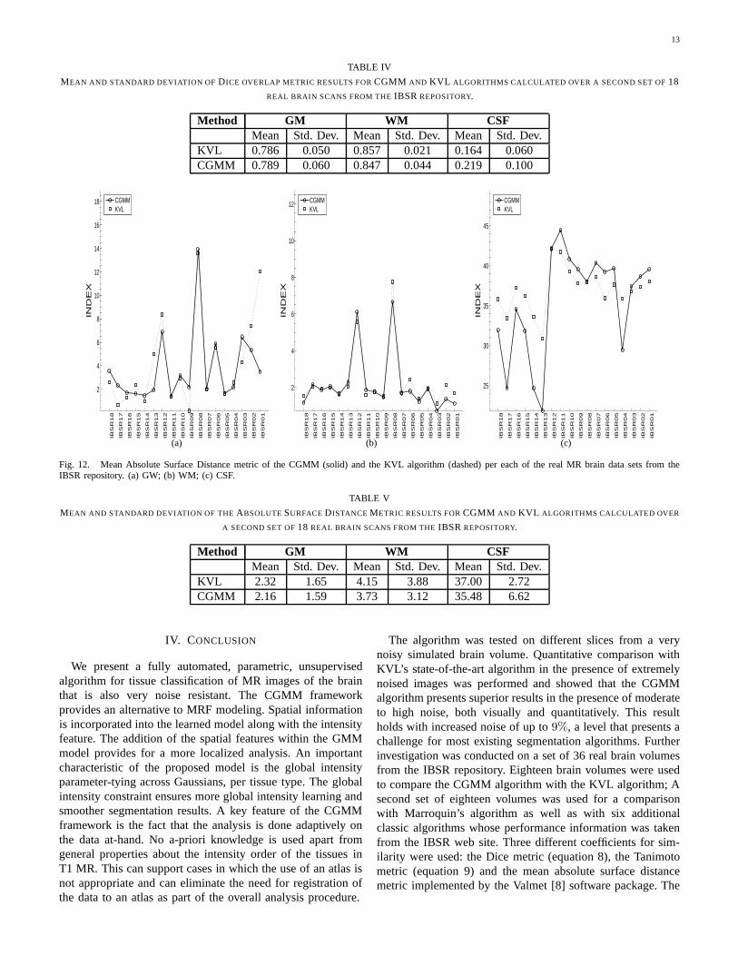
The Dice overlap metric is widely used in the literature (e.g[18], [13]) but it is by no means claimed to be the most suitablemetric for comparing performance of different segmentationalgorithms. In particular, the Dice metric depends on the sizeand the shape complexity of a given object and is relatedto the image sampling. Assuming that most of the errorsoccur at an object boundaries, small objects are penalizedand get a much lower score than large objects. No consensuscurrently exists regarding a necessary and sufficient set ofmeasures for segmentation performance characterization.In arecently published work, theMean absolute surface distancemetric (which is based on the Hausdorff distance metric [1])is suggested to compare different MR brain segmentationresults [8]. Figure 12 shows a comparison between the CGMMmethod and KVL’s algorithm, based on the mean absolutesurface distance metric as implemented by the VALMETsoftware package8 [8]. The results are summarized in Table V.Using this metric, a lower value means better segmentation.Asseen, the standard deviation of both algorithms is considerablyhigher than the differences in their average values. Thus, wecan only say that the two algorithms show a comparableperformance according to the mean absolute surface distancemetric.

8freely available at http://www.ia.unc.edu/dev/download/valmet/index.htm

12

0

0.1

0.2

0.3

0.4

0.5

0.6

0.7

0.8

0.9

1

IND

EX

205_

3

191_

3

112_

2

111_

2

110_

3

100_

23

17_3

16_3

15_3

13_3

12_3

11_3

8_4

7_8

6_10

5_8

2_4

1_24

CGMMamapbmapfuzzymapmlctskmmarro

(a)

0.1

0.2

0.3

0.4

0.5

0.6

0.7

0.8

0.9

1

IND

EX

205_

3

191_

3

112_

2

111_

2

110_

3

100_

23

17_3

16_3

15_3

13_3

12_3

11_3

8_4

7_8

6_10

5_8

2_4

1_24

CGMMamapbmapfuzzymapmlctskmmarro

(b)

Fig. 10. Tanimoto’s performance metric for different segmentation algorithms on different real brain MR scans from theIBSR repository. The bold linecorresponds to our algorithm. (a) WM; (b) GM.

TABLE III

MEAN AND STANDARD DEVIATION OF TANIMOTO ’ S OVERLAP METRIC FOR VARIOUS SEGMENTATION METHODS, CALCULATED OVER A FIRST SET OF18

BRAIN SCANS FROM THEIBSR REPOSITORY.

Method (abbr) Source GM WMMean Std. Dev. Mean Std. Dev.

adaptive MAP (amap) IBSR 0.57 0.13 0.58 0.17biased MAP (bmap) ” 0.56 0.17 0.58 0.21fuzzy c-means (fuzzy) ” 0.47 0.11 0.58 0.19Maximum a Posteriori Probability (map) ” 0.55 0.16 0.57 0.20tree-structure k-means (tskm) ” 0.48 0.12 0.58 0.19Maximum-Likelihood (mlc) ” 0.54 0.16 0.57 0.20Marroquin (marro) [18] 0.66 0.10 0.68 0.10Constrained GMM (CGMM) 0.68 0.04 0.66 0.06

0.7

0.75

0.8

0.85

0.9

IND

EX

IBS

R18

IBS

R17

IBS

R16

IBS

R15

IBS

R14

IBS

R13

IBS

R12

IBS

R11

IBS

R10

IBS

R09

IBS

R08

IBS

R07

IBS

R06

IBS

R05

IBS

R04

IBS

R03

IBS

R02

IBS

R01

CGMMKVL

(a)

0.65

0.7

0.75

0.8

0.85

0.9

IND

EX

IBS

R18

IBS

R17

IBS

R16

IBS

R15

IBS

R14

IBS

R13

IBS

R12

IBS

R11

IBS

R10

IBS

R09

IBS

R08

IBS

R07

IBS

R06

IBS

R05

IBS

R04

IBS

R03

IBS

R02

IBS

R01

CGMMKVL

(b)

0.05

0.1

0.15

0.2

0.25

0.3

0.35

0.4

0.45

0.5

IND

EX

IBS

R18

IBS

R17

IBS

R16

IBS

R15

IBS

R14

IBS

R13

IBS

R12

IBS

R11

IBS

R10

IBS

R09

IBS

R08

IBS

R07

IBS

R06

IBS

R05

IBS

R04

IBS

R03

IBS

R02

IBS

R01

CGMMKVL

(c)

Fig. 11. Dice overlap metric of the CGMM (solid) and the KVL algorithm (dashed) per each of the real MR brain data sets from the IBSR repository. (a)WM; (b) GM; (c) CSF.

13

TABLE IV

MEAN AND STANDARD DEVIATION OF DICE OVERLAP METRIC RESULTS FORCGMM AND KVL ALGORITHMS CALCULATED OVER A SECOND SET OF18

REAL BRAIN SCANS FROM THEIBSR REPOSITORY.

Method GM WM CSFMean Std. Dev. Mean Std. Dev. Mean Std. Dev.

KVL 0.786 0.050 0.857 0.021 0.164 0.060CGMM 0.789 0.060 0.847 0.044 0.219 0.100

2

4

6

8

10

12

14

16

18

IND

EX

IBS

R18

IBS

R17

IBS

R16

IBS

R15

IBS

R14

IBS

R13

IBS

R12

IBS

R11

IBS

R10

IBS

R09

IBS

R08

IBS

R07

IBS

R06

IBS

R05

IBS

R04

IBS

R03

IBS

R02

IBS

R01

CGMMKVL

(a)

2

4

6

8

10

12

IND

EX

IBS

R18

IBS

R17

IBS

R16

IBS

R15

IBS

R14

IBS

R13

IBS

R12

IBS

R11

IBS

R10

IBS

R09

IBS

R08

IBS

R07

IBS

R06

IBS

R05

IBS

R04

IBS

R03

IBS

R02

IBS

R01

CGMMKVL

(b)

25

30

35

40

45

IND

EX

IBS

R18

IBS

R17

IBS

R16

IBS

R15

IBS

R14

IBS

R13

IBS

R12

IBS

R11

IBS

R10

IBS

R09

IBS

R08

IBS

R07

IBS

R06

IBS

R05

IBS

R04

IBS

R03

IBS

R02

IBS

R01

CGMMKVL

(c)

Fig. 12. Mean Absolute Surface Distance metric of the CGMM (solid) and the KVL algorithm (dashed) per each of the real MR brain data sets from theIBSR repository. (a) GW; (b) WM; (c) CSF.

TABLE V

MEAN AND STANDARD DEVIATION OF THE ABSOLUTESURFACEDISTANCE METRIC RESULTS FORCGMM AND KVL ALGORITHMS CALCULATED OVER

A SECOND SET OF18 REAL BRAIN SCANS FROM THEIBSR REPOSITORY.

Method GM WM CSFMean Std. Dev. Mean Std. Dev. Mean Std. Dev.

KVL 2.32 1.65 4.15 3.88 37.00 2.72CGMM 2.16 1.59 3.73 3.12 35.48 6.62

IV. CONCLUSION

We present a fully automated, parametric, unsupervisedalgorithm for tissue classification of MR images of the brainthat is also very noise resistant. The CGMM frameworkprovides an alternative to MRF modeling. Spatial informationis incorporated into the learned model along with the intensityfeature. The addition of the spatial features within the GMMmodel provides for a more localized analysis. An importantcharacteristic of the proposed model is the global intensityparameter-tying across Gaussians, per tissue type. The globalintensity constraint ensures more global intensity learning andsmoother segmentation results. A key feature of the CGMMframework is the fact that the analysis is done adaptively onthe data at-hand. No a-priori knowledge is used apart fromgeneral properties about the intensity order of the tissuesinT1 MR. This can support cases in which the use of an atlas isnot appropriate and can eliminate the need for registrationofthe data to an atlas as part of the overall analysis procedure.

The algorithm was tested on different slices from a verynoisy simulated brain volume. Quantitative comparison withKVL’s state-of-the-art algorithm in the presence of extremelynoised images was performed and showed that the CGMMalgorithm presents superior results in the presence of moderateto high noise, both visually and quantitatively. This resultholds with increased noise of up to9%, a level that presents achallenge for most existing segmentation algorithms. Furtherinvestigation was conducted on a set of 36 real brain volumesfrom the IBSR repository. Eighteen brain volumes were usedto compare the CGMM algorithm with the KVL algorithm; Asecond set of eighteen volumes was used for a comparisonwith Marroquin’s algorithm as well as with six additionalclassic algorithms whose performance information was takenfrom the IBSR web site. Three different coefficients for sim-ilarity were used: the Dice metric (equation 8), the Tanimotometric (equation 9) and the mean absolute surface distancemetric implemented by the Valmet [8] software package. The

14

real brain volumes contain moderate thermal noise effects.Results show a significantly better performance of the CGMMframework as compared with the six segmentation algorithmsprovided as results in the IBSR site (Figure 11). The CGMMframework performed comparably to the Marroquin algorithm(Figure 11) as well as to the KVL algorithm (Figure 12) onthe real volumes.

The algorithm stability and consistency over a wide rangeof initial values was demonstrated. The processing time ofthe algorithm depends on the number of Gaussians which areused to model the brain data set as well as on the number ofvoxels in the image. The number of Gaussians is determinedin the initialization stage, as a by-product of the initializationparameters, noise level and tissue’s complexity. Using thedefault initialization parameters on the first set of 18 realbrainvolumes, the average processing time was 7 minutes for asingle brain volume, executed on a single 3.0GHz pentium4processor of a PC machine, with 1Gbyte memory.

The CGMM framework combines local spatial informationwith global intensity modeling. The grouping of Gaussianshas a resemblance to using a Markov Random Field model.The main difference is that the intensity information is linkedadaptively and globally within the image, in contrast to a MRFmodel that integrates information from the nearest neighborsonly and in predetermined neighborhoods. These differencesmay be the reason for the improved segmentation results withdecreased tissue region granularity in the presence of extremenoise.

Eliminating the need for an anatomical atlas provides theopportunity to apply the CGMM framework to diseased brainsand neonatal brains as well as to additional organs (ab-domen,chest, etc). Furthermore, the algorithm can be appliedto a subset of the full volume or even to 2D images. Currentlywe are working on an extension of the model to incorporateintensity inhomogeneities as well as to support multi-channeldata.

REFERENCES

[1] N. Aspert, D. Santa-Cruz, and T. Ebrahimi. Mesh: measuring errorsbetween surfaces using the Hausdorff distance. InICME 2208:1, pages705–708. IEEE, 2002.

[2] C. A. Cocosco, V. Kollokian, R. K. Kwan, and A. C. Evans. Brainweb:online interface to a 3D MRI simulated brain database.Neuroimage,5(4), 1997.

[3] Ctr. Morphometric Anal. [Online]. IBSR Internet brain segmenta-tion repository. tech. rep. http://neuro-www.mgh.harvard.edu/cma/ibsr/,2000.

[4] A. P. Dempster, N. M. Laird, and D. B. Rubin. Maximum likelihoodfrom incomplete data via the EM algorithm.Journal of the RoyalStatistical Society, (39):1–38, 1977.

[5] L. R. Dice. Measures of the amount of ecologic association betweenspecies.Ecology, 26(3):297–302, 1945.

[6] R. O. Duda, P. E. Hart, and D. G. Stork.Pattern Classification. WileyInterscience, 2001.

[7] G. Dugas-Phocion, M.Angel Gonzalez Ballester, G. Malandain, C. Le-brun, and N. Ayache. Improved EM-based tissue segmentationandpartial volume effect quantification in multi-sequence brain MRI. InInternational Conference on Medical Image Computing and ComputerAssisted Intervention (MICCAI), pages 26–33, 2004.

[8] G. Gerig, M. Jomier, and M. Chakos. Valmet: A new validation toolfor assessing and improving 3D object segmentation. InLNCS 2208,pages 516–528. International Conference on Medical Image Computingand Computer Assisted Intervention (MICCAI), 2001.

[9] K. Held, E. R. Kops, B. J. Krause, W. M. Wells III, R. Kikinis, andH. Muller-Gartner. Markov random field segmentation of brain MRimages.IEEE Trans. Med. Imaging, 16(6):878–886, 1997.

[10] K. V. Leemput. Expectation-Maximization segmentation (EMS).http://www.medicalimagecomputing.com/EMS/, 2001.

[11] T. Kapur, W. E. Grimson, W. M. Wells, and R. Kikinis. Segmentationof brain tissue from magnetic resonance images.Med Image Anal.,1(2):109–27, 1996.

[12] K. V. Leemput, F. Maes, D. Vandermeulen, A. C. F. Colchester, andP. Suetens. Automated segmentation of multiple sclerosis lesions bymodel outlier detection. IEEE Trans. Med. Imaging, 20(8):677–688,2001.

[13] K. V. Leemput, F. Maes, D. Vandermeulen, and P. Suetens.Automatedmodel-based tissue classification of MR images of the brain.IEEETrans. Med. imaging, 18(10):897–908, 1999.

[14] K. V. Leemput, F. Maes, D. Vandermeulen, and P. Suetens.A unifyingframework for partial volume segmentation of brain MR images. IEEETrans. Med. Imaging, 22(1):105–119, 2003.

[15] S. Z. Li. Markov random field modeling in computer vision. Springer-Verlag, 1995.

[16] A. Macovski. Noise in MRI.Magn. Reson. Med., 36(3):494–7, 1996.[17] F. Maes, A. Collignon, D. Vandermeulen, G. Marchal, andP. Suetens.

Multimodality image registration by maximization of mutual informa-tion. IEEE Trans. Med. Imaging, 16(2):187–198, 1997.

[18] J. L. Marroquin, B. C. Vemuri, S. Botello, F. Calderon, andA. Fernandez-Bouzas. An accurate and efficient bayesian method forautomatic segmentation of brain MRI.IEEE Trans. Med. imaging,21(8):934–45, 2002.

[19] T. McInerney and D. Terzopoulos. Medical image segmentation usingtopologically adaptable surfaces. InProceedings of the First Joint Con-ference on Computer Vision, Virtual Reality and Robotics inMedicineand Medial Robotics and Computer-Assisted Surgery, pages 23–32.Springer-Verlag, 1997.

[20] D. L. Pham. Spatial models for fuzzy clustering.CVIU, 84(2):285–297,2001.

[21] D. L. Pham, C. Xu, and J. L. Prince. Current methods in medical imagesegmentation.Annual Review of Biomedical Engineering, 2:315–337,2000.

[22] M. Prastawa, J. Gilmore, W. Lin, and G. Gerig. Automaticsegmentationof neonatal brain MRI. InInternational Conference on Medical ImageComputing and Computer Assisted Intervention (MICCAI), pages 10–17,2004.

[23] T. Rohlfing and C. R. Maurer Jr. Nonrigid image registration in shared-memory multiprocessor environments with application to brains, breasts,and bees.IEEE Transactions on Information Technology in Biomedicine,7(1):16–25, 2003.

[24] A. Ruf, H. Greenspan, and J. Goldberger. Tissue classification of noisyMR brain images using constrained GMM.International Conferenceon Medical Image Computing and Computer Assisted Intervention(MICCAI), 2005.

[25] W. Wells, R. Kikinis, W. Grimson, and F. Jolesz. Adaptive segmentationof MRI data. IEEE Trans. Med. imaging, 15:429–42, 1996.

[26] Z. Xue, D. Shen, and C. Davatzikos. Classic: Consistentlongitudinalalignment and segmentation for serial image computing. InIPMI,volume 3565, pages 101–113, Jul 2005.

[27] Y. Zhang, M. Brady, and S. Smith. Segmentation of brain MR imagesthrough a hidden markov random field model and the Expectation-Maximization algorithm.IEEE Trans. Med. imaging, 20(1):45–57, 2001.

[28] A. P. Zijdenbos and B. M. Dawant. Brain segmentation andwhitematter lesion detection in MR images.Critical Reviews in BiomedicalEngineering, 22(5-6):401–65, 1994.